銷售預測陳得發教授國立中山大學企業管理學系

銷售預測銷售預測

陳得發教授陳得發教授

國立中山大學企業管理學系國立中山大學企業管理學系

一、市場分析一、市場分析

1. 1. 需求者分析（消費者或企業）需求者分析（消費者或企業） 11 ）需求者類別）需求者類別 22 ）需求者消費習性（價格導向、品質導向、）需求者消費習性（價格導向、品質導向、形象導向）形象導向） 33 ）需求者經濟狀況（財力、購買力））需求者經濟狀況（財力、購買力） 44 ）需求者使用量）需求者使用量


2. 2. 供應者分析（競爭者）供應者分析（競爭者） 11 ）供應者產能、產量）供應者產能、產量 22 ）供應者產品特性）供應者產品特性 33 ）供應者財力與市場地位）供應者財力與市場地位 44 ）供應者銷售通路）供應者銷售通路 55 ）供應者原物料來源）供應者原物料來源 66 ）供應者的媒體資源）供應者的媒體資源 77 ）供應者的價格策略）供應者的價格策略


3. 3. 替代產品分析（潛在競爭者）替代產品分析（潛在競爭者） 11 ）潛在競爭者產能、產量）潛在競爭者產能、產量 22 ）潛在競爭者產品特性）潛在競爭者產品特性 33 ）潛在競爭者財力與市場地位）潛在競爭者財力與市場地位 44 ）潛在競爭者銷售通路）潛在競爭者銷售通路 55 ）潛在競爭者原物料來源）潛在競爭者原物料來源 66 ）潛在競爭者的媒體資源）潛在競爭者的媒體資源 77 ）潛在競爭者的價格策略）潛在競爭者的價格策略


4. 4. 通路分析通路分析 11 ）通路商經銷的產品類別）通路商經銷的產品類別 22 ）通路商的分佈地點）通路商的分佈地點 33 ）通路商的配銷能力）通路商的配銷能力 44 ）通路商的促銷意願與能力）通路商的促銷意願與能力 55 ）通路商的收費方式）通路商的收費方式


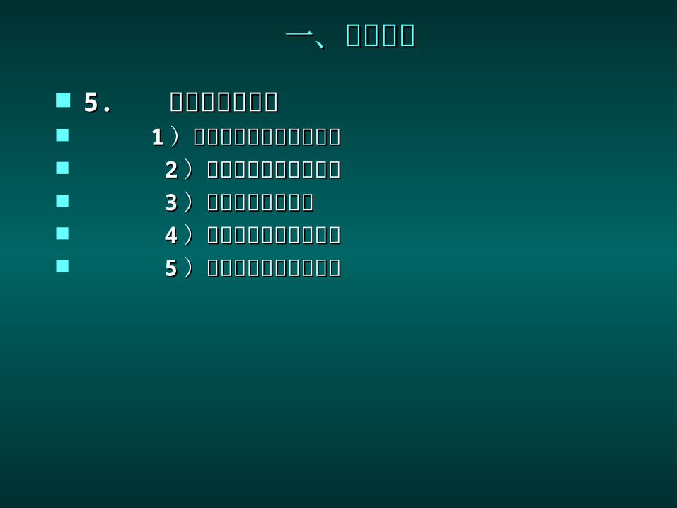
5. 5. 上游供應者分析上游供應者分析 11 ）上游供應商的產能與產量）上游供應商的產能與產量 22 ）上游供應商的配送能力）上游供應商的配送能力 33 ）上游供應商的財力）上游供應商的財力 44 ）上游供應商的產品品質）上游供應商的產品品質 55 ）上游供應商的價格策略）上游供應商的價格策略


6. 6. 總體經濟環境分析總體經濟環境分析 11 ）過去的總體經濟）過去的總體經濟 22 ）目前的總體經濟）目前的總體經濟 33 ）未來的總體經濟）未來的總體經濟

二、時間數列分析二、時間數列分析

1. 1. 組成因素組成因素 11 ）趨勢因素）趨勢因素 22 ）週期循環）週期循環 33 ）季節循環）季節循環 44 ）不規則因素）不規則因素

(( 時間數列分析詳細內容可參考統計書籍的預測章節時間數列分析詳細內容可參考統計書籍的預測章節 ))

(( 本文資料攫取自本文資料攫取自 Ch. 18 Forecasting, Ch. 18 Forecasting,

By Anderson: Statistics for Business and By Anderson: Statistics for Business and Economics)Economics)

2. 2. 平滑法平滑法 11 ）移動平均平滑法）移動平均平滑法

• 我們用最近的我們用最近的 n n 個資料值當作下一期的預測值個資料值當作下一期的預測值• 移動平均值的計算方式如下：移動平均值的計算方式如下：

Moving Average = Moving Average = (most recent (most recent nn data data values)/values)/nn


2. 2. 平滑法平滑法 22 ）加權移動平均平滑法）加權移動平均平滑法

• 這個方法必須決定前幾期資料的權重，然後計算加這個方法必須決定前幾期資料的權重，然後計算加權平均值作為下一期的預測值。權平均值作為下一期的預測值。

• 例如一個例如一個 3 3 期加權移動平均值的計算方式可以表期加權移動平均值的計算方式可以表達如下：達如下：

FFtt + 1 + 1 = = ww11((YYtt - 2 - 2) + ) + ww22((YYtt - 1 - 1) + ) + ww33((YYtt))

其中，權重的和其中，權重的和 ((w w values) values) 為為 1.1.



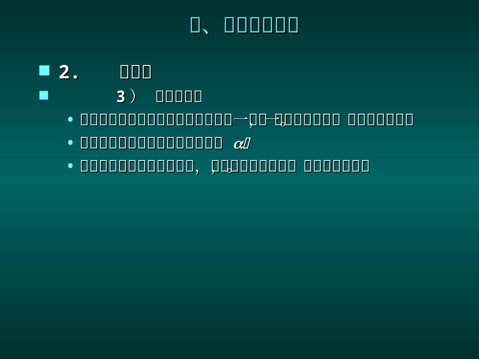
2. 2. 平滑法平滑法 33 ）指數平滑法）指數平滑法

• 指數平滑法可視為加權移動平均法的一種，我們只指數平滑法可視為加權移動平均法的一種，我們只給最近一期的資料權重。給最近一期的資料權重。

• 最近一期資料的權重稱為平滑常數最近一期資料的權重稱為平滑常數。。• 其餘資料的權重會自動計算，而且以指數的比例，其餘資料的權重會自動計算，而且以指數的比例，

越遠的會越小。越遠的會越小。

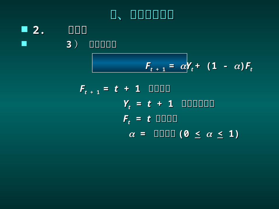
二、時間數列分析二、時間數列分析 2. 2. 平滑法平滑法 33 ）指數平滑法）指數平滑法

FFtt + 1 + 1 = = YYt t + (1 - + (1 - ))FFtt

FFtt + 1 + 1 = = tt + 1 + 1 的預測值的預測值 YYtt = = tt + 1 + 1 的實際觀察值的實際觀察值 FFtt = = t t 的預測值的預測值 = = 平滑常數平滑常數 (0 (0 << << 1) 1)

Example: Executive Seminars, Inc.Example: Executive Seminars, Inc.

Executive Seminars specializes in conductingExecutive Seminars specializes in conducting

management development seminars. In order to management development seminars. In order to betterbetter

plan future revenues and costs, management plan future revenues and costs, management would likewould like

to develop a forecasting model for their “Timeto develop a forecasting model for their “Time

Management” seminar.Management” seminar.

Enrollments for the past ten “TM” seminars are:Enrollments for the past ten “TM” seminars are:

(oldest)(oldest) (newest) (newest)

SeminarSeminar 11 22 33 44 55 66 77 88 99 1010

Enroll. Enroll. 3434 4040 3535 3939 4141 3636 3333 3838 4343 4040


Exponential SmoothingExponential Smoothing

Let Let = .2, = .2, FF1 1 = = YY1 1 = 34= 34

FF2 2 = = YY11 + (1 - + (1 - ))FF11

= .2(34) + .8(34)= .2(34) + .8(34) = 34= 34

FF3 3 = = YY22 + (1 - + (1 - ))FF22

= .2(40) + .8(34)= .2(40) + .8(34) = 35.20= 35.20

FF4 4 = = YY33 + (1 - + (1 - ))FF33

= .2(35) + .8(35.20)= .2(35) + .8(35.20) = 35.16 = 35.16

. . . and so on. . . and so on


SeminarSeminar Actual EnrollmentActual Enrollment Exp. Sm. Exp. Sm. ForecastForecast

11 3434 34.0034.0022 4040 34.0034.0033 3535 35.2035.2044 3939 35.1635.1655 4141 35.9335.9366 3636 36.9436.9477 3333 36.7636.7688 3838 36.0036.0099 4343 36.4036.401010 4040 37.7237.721111 Forecast for the next seminarForecast for the next seminar = =

38.1838.18

3. 3. 趨勢預測趨勢預測

TTtt = = bb00 + + bb11tt

TTtt = = t t 期的趨勢值期的趨勢值 bb00 = = 趨勢線的截距趨勢線的截距 bb1 1 = = 趨勢線的斜率趨勢線的斜率 tt = = 時期時期 Note: Note: tt is the independent variable. is the independent variable.


計算斜率計算斜率 ((bb11) ) 和截距和截距 ((bb00))

bb11 = = tYtYtt - ( - (t t YYtt)/)/nn

t t 22 - ( - (t t ))22//nn

bb00 = (= (YYtt//nn) - ) - bb11tt//n n = = YY - - bb11tt

wherewhere

YYtt = = t t 期的實際觀測值期的實際觀測值 n = n = 時間數列的期數時間數列的期數

趨勢預測的作法趨勢預測的作法

Example: Sailboat Sales, Inc.Example: Sailboat Sales, Inc.

Sailboat Sales is a major marine dealer in Sailboat Sales is a major marine dealer in Chicago. The firm has experienced Chicago. The firm has experienced tremendous sales growth in the past several tremendous sales growth in the past several years. Management would like to develop a years. Management would like to develop a forecasting method that would enable them to forecasting method that would enable them to better control inventories.better control inventories.

The annual sales, in number of boats, for The annual sales, in number of boats, for one particular sailboat model for the past five one particular sailboat model for the past five years are:years are:

YearYear 11 22 33 44 55

SalesSales 1111 1414 2020 2626 3434

Linear Trend EquationLinear Trend Equation

tt YYtt tYtYtt t t 22

11 1111 1111 1 1

22 1414 2828 4 4

33 2020 6060 9 9

44 2626 104104 1616

55 3434 170170 2525

TotalTotal 1515 105105 373373 5555


Trend ProjectionTrend Projection

bb1 1 = 373 - (15)(105)/5 = 5.8 = 373 - (15)(105)/5 = 5.8

55 - (15)55 - (15)22/5/5

bb00 = 105/5 - 5.8(15/5) = 3.6 = 105/5 - 5.8(15/5) = 3.6

TTtt = 3.6 + 5.8 = 3.6 + 5.8tt

TT66 = 3.6 + 5.8(6) = 38.4 = 3.6 + 5.8(6) = 38.4


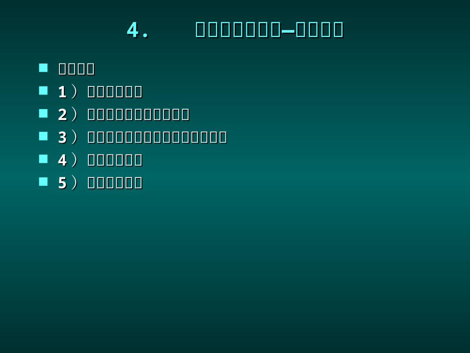
4. 4. 趨勢和季節因素趨勢和季節因素——乘法模式乘法模式操作步驟操作步驟 11 ）計算季節指數）計算季節指數 22 ）去掉時間數列的季節因素）去掉時間數列的季節因素 33 ）利用去掉季節因素的數列來找趨勢）利用去掉季節因素的數列來找趨勢 44 ）加入季節因素）加入季節因素 55 ）加入循環因素）加入循環因素

4. 4. 趨勢和季節因素趨勢和季節因素——乘法模式乘法模式

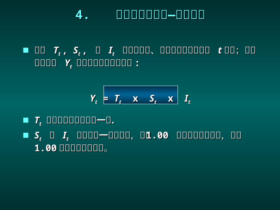
利用利用 TTt t , , SSt t , , 和和 IItt 來代表趨勢、季節和不規則因素來代表趨勢、季節和不規則因素在在 tt 的值；把時間數列的的值；把時間數列的 YYt t 用下列的乘法模式表用下列的乘法模式表示示 ::

YYtt = = TTtt xx SStt xx IItt

TTtt 的衡量單位和觀察值一樣的衡量單位和觀察值一樣 ..

SStt 和和 IItt 的衡量是一種比例值，大於的衡量是一種比例值，大於 1.00 1.00 表示在趨表示在趨勢的上方，小於勢的上方，小於 1.001.00 表示在趨勢的下方。表示在趨勢的下方。

季節指數的計算季節指數的計算

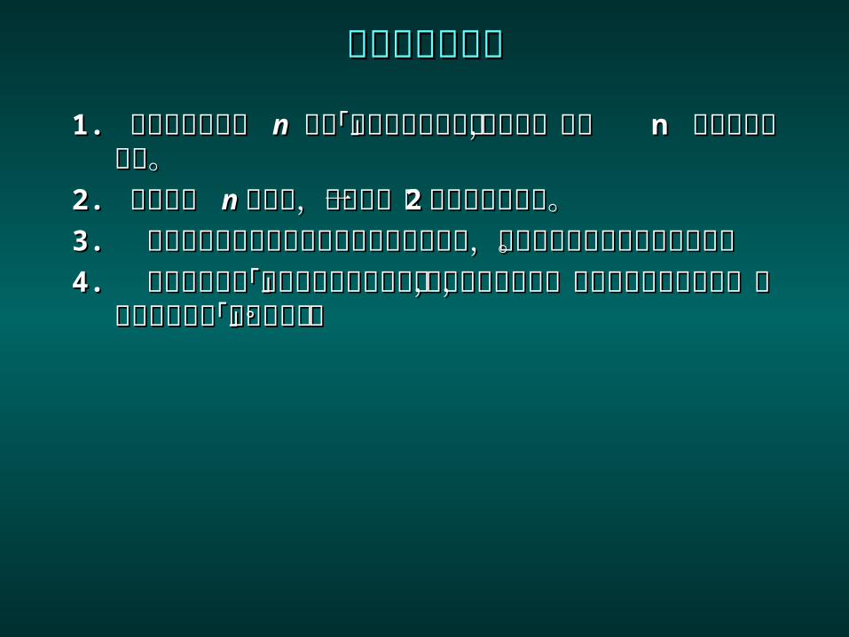
1. 1. 假如週期長度為假如週期長度為 n n 運用「中央移動平均值」的算法運用「中央移動平均值」的算法，算出，算出 n n 期的移動平均值。期的移動平均值。

2. 2. 假如週期假如週期 nn 是偶數，要再算一次是偶數，要再算一次 22 期的移動平均值期的移動平均值。。

3. 3. 將原始的觀察值除以對應的中央移動平均值，來顯將原始的觀察值除以對應的中央移動平均值，來顯示其季節和不規則的效應。示其季節和不規則的效應。

4. 4. 將相同季節的「季節和不規則效應值」加總求其平將相同季節的「季節和不規則效應值」加總求其平均值，即可消除不規則效應，而得到各季節的「季節均值，即可消除不規則效應，而得到各季節的「季節指數」。指數」。

將時間數列消除季節因素將時間數列消除季節因素

找出季節指數的目的，是要將時間數列的季節因素消找出季節指數的目的，是要將時間數列的季節因素消除。除。

將原始時間數列除以期季節指數，所得結果即為無季將原始時間數列除以期季節指數，所得結果即為無季節因素的時間數列。節因素的時間數列。

利用無季節因素的數據，針對各期的資料就可以做很利用無季節因素的數據，針對各期的資料就可以做很多重要的比較分析。多重要的比較分析。

利用無季節因素的時間數列來找出長期趨勢利用無季節因素的時間數列來找出長期趨勢要找出直線的趨勢，我們可用線性回歸分析的方法，要找出直線的趨勢，我們可用線性回歸分析的方法，從無季節因素的時間數列中找出其直線方程式。從無季節因素的時間數列中找出其直線方程式。

找出來的直線方程式可以用來做長期趨勢預測。找出來的直線方程式可以用來做長期趨勢預測。

季節調整季節調整

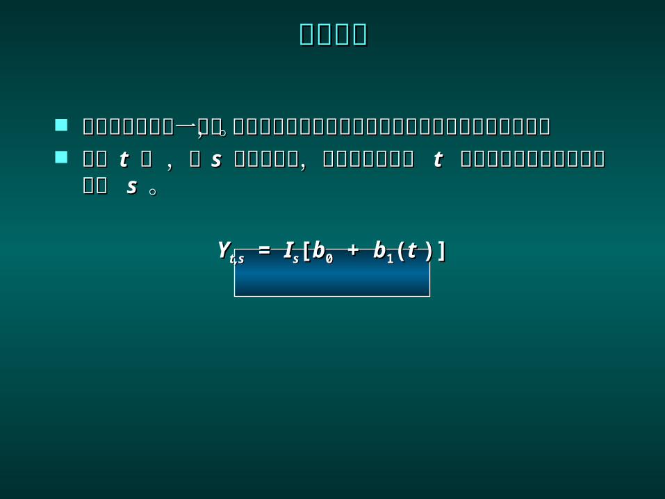
預測分析的最後一步，是將長期趨勢預測的各季預測預測分析的最後一步，是將長期趨勢預測的各季預測值再用季節指數來調整。值再用季節指數來調整。

對第對第 t t 期，第期，第 s s 季的預測值，是將趨勢預測第季的預測值，是將趨勢預測第 t t 期的值乘以其對應的季節指數期的值乘以其對應的季節指數 s s 。。

YYt,st,s = = IIss[[bb00 + + bb11((t t )])]

Example: Eastern Athletic SuppliesExample: Eastern Athletic Supplies

Management of EAS would like to develop aManagement of EAS would like to develop a

quarterly sales forecast for one of their tennis quarterly sales forecast for one of their tennis rackets. rackets.

Sales of tennis rackets is highly seasonal and Sales of tennis rackets is highly seasonal and hence anhence an

accurate quarterly forecast could aid accurate quarterly forecast could aid substantially insubstantially in

ordering raw material used in manufacturing.ordering raw material used in manufacturing.

The quarterly sales data (000 units) for the The quarterly sales data (000 units) for the previousprevious

three years is shown on the next slide.three years is shown on the next slide.

Year QuarterYear Quarter SalesSales 11 1 1 33

22 99 33 66 44 22

22 1 1 44 22 1111 33 88 44 33

33 1 1 55 22 1515 33 1111 44 33


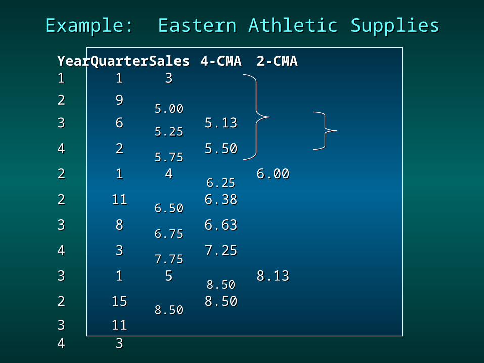
YearYearQuarterQuarterSalesSales 4-CMA4-CMA 2-CMA 2-CMA11 11 33

22 995.005.00

33 665.255.25

5.135.13

44 225.755.75

5.505.50

22 11 446.256.25

6.006.00

22 11116.506.50

6.386.38

33 886.756.75

6.636.63

44 337.757.75

7.257.25

33 11 558.508.50

8.138.13

22 15158.508.50

8.508.50

33 111144 33


YearYear QuarterQuarter Sales 2-CMASales 2-CMA Seas- Seas-IrregIrreg

11 11 3322 9933 66 5.135.13 1.171.1744 22 5.505.50 0.360.36

22 11 44 6.006.00 0.670.6722 1111 6.386.38 1.721.7233 88 6.636.63 1.211.2144 33 7.257.25 0.410.41

33 11 55 8.138.13 0.620.6222 1515 8.508.50 1.761.7633 111144 33


QuarterQuarterSeas-Irreg ValuesSeas-Irreg ValuesSeas. IndexSeas. Index11 0.67, 0.620.67, 0.62 0.650.6522 1.72, 1.761.72, 1.76 1.741.7433 1.17, 1.211.17, 1.21 1.191.1944 0.36, 0.410.36, 0.41 0.390.39 Total =Total =

3.973.97

Seas.IndexSeas.Index Adj. Factor Adj. FactorAdj.Seas.IndexAdj.Seas.Index0.650.65 4/3.97 4/3.97 .655 .655 1.741.74 4/3.97 4/3.97 1.7531.753

1.191.19 4/3.97 4/3.97 1.1991.1990.390.39 4/3.97 4/3.97 .393.393

Total = 4.000 Total = 4.000


YearYearQuarterQuarterSalesSalesSeas.IndexSeas.Index Deseas.SalesDeseas.Sales

11 11 33 .655.655 4.58 4.5822 99 1.7531.753 5.13 5.1333 66 1.1991.199 5.00 5.0044 22 .393.393 5.09 5.09

22 11 44 .655.655 6.11 6.1122 1111 1.7531.753 6.27 6.2733 88 1.1991.199 6.67 6.6744 33 .393.393 7.63 7.63

33 11 55 .655.655 7.63 7.6322 1515 1.7531.753 8.56 8.5633 1111 1.1991.199 9.17 9.1744 33 .393.393 7.63 7.63



Trend ProjectionTrend Projection

TTtt = 4.066 + .3933 = 4.066 + .3933tt

TT1313 = 4.066 + .3993(13) = 9.1789 = 4.066 + .3993(13) = 9.1789

Using the trend component only, Using the trend component only, we would we would forecast sales of 9,179 tennis rackets forecast sales of 9,179 tennis rackets for for period 13 (year 4, quarter 1).period 13 (year 4, quarter 1).


Seasonal AdjustmentsSeasonal Adjustments

PeriodPeriod TrendTrend SeasonalSeasonal QuarterlyQuarterly

tt Forec. Forec. IndexIndex Forecast Forecast

13 9,17913 9,179 .655 .655 6,012 6,012

14 9,57214 9,572 1.753 1.753 16,78016,780

15 9,96615 9,966 1.199 1.199 11,94911,949

1616 10,35910,359 .393 .393 4,071 4,071

根據月份資料的預測模式根據月份資料的預測模式

很多企業會做月份的銷售預測，這時候只需將前述的很多企業會做月份的銷售預測，這時候只需將前述的方法作一些小修改即可。方法作一些小修改即可。

• 將前述將前述 44 季的移動平均值改為季的移動平均值改為 1212 個月的移動平均個月的移動平均值值

• 再用類似的方法算出再用類似的方法算出 1212 個月的「月指數」。個月的「月指數」。• 其餘的運算流程都一樣。其餘的運算流程都一樣。

乘法模式可加以擴充，把週期循環因素加進來，將週乘法模式可加以擴充，把週期循環因素加進來，將週期循環因素以長期趨勢的百分比來顯示。期循環因素以長期趨勢的百分比來顯示。

然而，要把週期循環因素放進來，有一些困難的地方然而，要把週期循環因素放進來，有一些困難的地方 ::

• 一個週期可能要歷經很多年才完成，因此必須要有一個週期可能要歷經很多年才完成，因此必須要有相當長期的資料才能用來分析週期循環的現象。相當長期的資料才能用來分析週期循環的現象。

• 週期的長度常會變化。週期的長度常會變化。

週期循環因素週期循環因素

t t t t tY T C S I t t t t tY T C S I

三、迴歸分析三、迴歸分析

銷售值常會受到其他環境因素的影響，這時候可將銷銷售值常會受到其他環境因素的影響，這時候可將銷售值當作「應變數」，其他的相關環境因素作為「自售值當作「應變數」，其他的相關環境因素作為「自變數」來進行回歸分析。變數」來進行回歸分析。

自變數可能包含下列資料或其組合自變數可能包含下列資料或其組合 ::

• 前期的銷售值前期的銷售值• 經濟或人口變數經濟或人口變數• 時間變數時間變數

迴歸分析迴歸分析

自我迴歸分析模式（自我迴歸分析模式（ autoregressive modelautoregressive model ））是迴歸分析的一種，其自變數是前期的觀測值。是迴歸分析的一種，其自變數是前期的觀測值。

因果分析預測模式（因果分析預測模式（ causal forecasting modelcausal forecasting model）則利用可能會影響銷售值的其他變數做自變數，來）則利用可能會影響銷售值的其他變數做自變數，來作迴歸分析，希望能找出銷售值變動的因果關係作迴歸分析，希望能找出銷售值變動的因果關係。。


對一個有對一個有 kk 個自變數的迴歸分析，我們通常使用以下的符個自變數的迴歸分析，我們通常使用以下的符號來表示號來表示 ::

YYtt = value of the time series in period = value of the time series in period tt

xx11tt = value of independent variable 1 in = value of independent variable 1 in period period tt

xx22tt = value of independent variable 2 in = value of independent variable 2 in period period tt

xxktkt = value of independent variable = value of independent variable kk in in period period tt


在預測冰箱的銷售時，我們可能會選用以下的五個自在預測冰箱的銷售時，我們可能會選用以下的五個自變數變數 ::

xx11tt = price of refrigerator in period = price of refrigerator in period tt

xx22tt = total industry sales in period = total industry sales in period tt - - 11

xx33tt = number of new-house building = number of new-house building permits permits in period in period tt - 1 - 1

xx44tt = population forecast for period = population forecast for period tt

xx55tt = advertising budget for period = advertising budget for period tt


nn 期的資料用來作迴歸分析，可以列表入下列的方式期的資料用來作迴歸分析，可以列表入下列的方式 ::

PeriodPeriod Time Series Value of Independent Variables Time Series Value of Independent Variables

((tt)) ((YYtt)) ( (xx11tt) () (xx22tt) () (xx33tt) . . () . . (xxktkt))

11 YY11 xx1111 xx2121 xx3131 . . . . xxkk11

22 YY22 xx1212 xx2222 xx3232 . . . . xxkk22

.. . . . . . . . . . . . . . . . . . . . . . . . . . . . . . .

nn Y Ynn x x11nn xx22nn xx33nn . . . . xxknkn

四、專家判斷法四、專家判斷法

Delphi MethodDelphi Method

• It is an attempt to develop forecasts It is an attempt to develop forecasts through “group consensus.”through “group consensus.”

• The goal is to produce a relatively The goal is to produce a relatively narrow spread of opinions within which narrow spread of opinions within which the majority of the panel of experts the majority of the panel of experts concur.concur.

Expert JudgmentExpert Judgment

• Experts individually consider information Experts individually consider information that they believe will influence the that they believe will influence the variable; then they combine their variable; then they combine their conclusions into a forecast.conclusions into a forecast.

• No two experts are likely to consider the No two experts are likely to consider the same information in the same way.same information in the same way.

銷 售 預 測 陳得發教授 國立中山大學企業管理學系

Documents

銷售預測陳得發教授國立中山大學企業管理學系