-Ï È Õ department of physics and …member.ipmu.jp/atsushi.nishizawa/study/phd_thesis.pdfi am...
TRANSCRIPT
SECONDARY ANISOTROPIES OF THE COSMIC MICROWAVEBACKGROUND RADIATION
— A CROSS CORRELATION STUDY OF THE REES-SCIAMA EFFECT WITH
WEAK LENSING
AND THE IMPLICATIONS FOR DARK ENERGY —
——————————————————————————————–
A DISSERTATION SUBMITTED TO
DEPARTMENT OF PHYSICS AND ASTROPHYSICS
NAGOYA UNIVERSITY
IN CANDIDACY FOR DEGREE OF DOCTOR OF PHILOSOPHY
——————————————————————————————–
Nishizawa Atsushi
DEPARTMENT OF PHYSICS AND ASTROPHYSICS NAGOYA UNIVERSITY
FUROCHO CHIKUSA NAGOYA CITY 464-8602, AICHI JAPAN
NAGOYA, DECEMBER 14 2007
Supervisor: Professor. Dr. SUGIYAMA NAOSHI
Co-Supervisor: Professor. Dr. SHIBAI HIROSHI
3
Abstract
Recent astronomical observations revealed a number of mysteries of our Universe. One
of the most prominent results is the accurate measurement of temperature fluctuations of
Cosmic Microwave Background(CMB) byWilkinson Microwave Anisotropy Probe (WMAP)
satellite. The observation suggests that our universe consists of 22% dark matter, 4%
baryons and that the spacial curvature is almost equal to zero, i.e. space is flat. This
implies the existence of 74% unknown energy components in the universe. In the late
1990’s, supernovae(SNe) observations were actively pursued. SNe observations measured
the luminosity distance, which depends on a cosmological model, specifically the expan-
sion history of the universe, between SNe and us. The SNe results suggest that our
universe has been undergoing accelerating expansion since 6 Gyr ago. Combination of
the CMB and SNe results suggest that the 74% unknown energy component causes the
apparent accelerated expansion of our universe. The cosmological constant, introduced
originally by Einstein to keep the universe static, well accounts for this phenomenon in
the simplest manner. Another important result of recent observations is large scale dis-
tribution of galaxies. Wide field and deep galaxy observations, such as 2dF and SDSS
surveys, measured the 3-dimensional distribution of galaxies. One of the most important
results from these observations is that the dark matter component is cold, i.e. the velocity
is small. Since the major component of the universe is Cold Dark Matter(CDM) and Λ,
the standard model of cosmology is called as ΛCDM.
Now an outstanding issue in cosmology may be ”What is dark energy ?” One ap-
proach is observating the integrated Sachs Wolfe (ISW) effect, or its non-linear extension,
the Rees-Sciama (RS) effect. When CMB photons pass through the large scale struc-
ture(LSS) of the universe, their energies are slightly shifted; When a photon falls into the
gravitational potential of LSS, it gains the energy, or blueshifts. Whereas when it climbs
up the potential well, it loses its energy, or redshifts. If the potential would not vary with
time during the photon passage, the amount of blueshift and redshift is equal and thus
the net effects are cancelled out. However, since the potential wells in general evolve with
time, the net energy gain or loss is expected. On large scales, the existence of dark energy
dilutes the potential well (ISW), while on small scales, gravitational collapse concentrates
the potential well (RS). Thus the temperatures in the direction where potentials exist
along the line of sight and in the direction where potentials do not exist along the line
of sight are different. The temperature fluctuations caused by the RS effect are gener-
ally very small, and direct detection is extremely difficult. However, it is expected that
the temperature fluctuations caused by the RS effect and underlying matter distribution
must have some correlation. We propose to use a statistical method; the cross-correlation
between the CMB and the matter distribution traced by weak lensing.
4
We calculate the cross-correlation power spectrum using large cosmological N -body
simulations and analytical models. There is no exact theory to describe the non-linearity
of the potential: We show that the higher order perturbation theory can be applicable
and a few phenomenological models show good agreement with the result of the N -body
simulations.
We find the cross-correlation of the RS and weak lensing provides a unique probe for
investigating non-linear evolution of density fluctuations on small scales. Moreover we
discover an interesting feature in the cross-correlation angular power spectrum. It shows
correlation on large scales while it shows anti-correlation on small scales. There exists
cross over point in the intermediate scale. This cross over point is sensitive to the energy
density and the nature of dark energy, especially to its equation of state. We conclude
that the cross over point can be a unique probe of dark energy.
5
Acknowledgments
I am grateful to professor Naoshi Sugiyama for the careful supervising. He always points outthe physically or mathematically unclear things in my statements. This largely helps me tounderstand cosmology and to improve my way of thinking. I think the encounter with Sugiyama-san is one of the happiest happening in my research life. I would like to express gratitude toprofessor Hiroshi Shibai. He is supportive for me to join the Akari FIS team. With his greathelps, I undergo many precious experiences in the Akari satellite operation and data reduction.I would never experience such an important tasks without Shibai-san’s kind supports. I shouldalso acknowledge professor Takahiko Matsubara. He used to be my supervisor for first threeyears in my graduated course at Nagoya University. He taught me a lot of knowledge aboutcosmology and mathematics. His statements are always mathematically exactly correct, andhe solves all the problems immediately that I was troubled. I learned from Matsubara-santhe importance and interests of mathematical derivations or understanding of the physics. Ipartially learn from professor Satoru Ikeuchi. I also acknowledge Ikeuchi-san. He gives me a lotof precious episodes on physics and natural science. Though these are not directly related tomy research, the way of thinking or way of see the nature becomes very good lessons for me.
I am also grateful to Professor Naoki Yoshida. He is always amiable for my discussion andquestion. Also I leaned from Yoshida-san much about the N -body simulation and numericalcalculation technique. Some of the result of this thesis and the paper is achieved with thesupport of Yoshida-san. He also gives me good opportunities to get to know the internationalresearchers and an encouragement of the collaboration work. Eiichiro Komatsu, the collaboratorhelps many times me to understand the non-linear theory, halo model and related statistics. Iacknowledge him so much. He always happily has discussions with me about any issues on thecosmology. Also his passion and faculty to the cosmology stimulates my motivation to pursue thePhD study. Ryuichi Takahashi, also one of my important collaborator helps my work throughthe N -body simulation. I also acknowledge him.
I would like to acknowledge David Spergel, Olivier Dore, Joseph Henawii. They give manyvaluable comments on our study and we can improve the paper significantly. Ravi Sheth gives mean unpublished his draft about momentum power spectrum using halo model. This greatly helpsme to understand the halo model descriptions. I am grateful to Ravi Sheth. I also acknowledgeAsantha Cooray. I discussed him at Nagoya and London and in e-mail many times. I learnedfrom him much about the integrated Sachs Wolfe effect and how to write so many papers in oneyear.
I would like to show my gratitude to the researchers, Yasushi Suto, Atsushi Taruya, MasahiroTakada, Takashi Hamana, Kouji Yoshikawa, Tsutomu Takeuchi, Hiroyuki Tashiro, and DavidPerkinson. Although I could not discuss them constantly but when I met them at the conferencesand workshops, they welcome my simple and honest questions.
Matsubara-san gives me chance to participate the Prioritised Study of Akari (ASTRO-F)related to the ISW analysis. I am also grateful to Richard Savage, the PI of this study. Shibai-san
6
also invites me to the Akari-FIS team and Akari-FIS data reduction team. I had an invaluableexperience through the Akari satellite operation and part of the data analysis. I would like toshow my gratitude to the project manager of Akari, Hiroshi Murakami, and professors HideoMatsuhara, Issei Yamamura, Shuji Matsuura, Tsuneo Kii, and the researchers, Mai Shirahata,Shin’ichiro Makiuchi and Shinki Oyabu at ISAS/JAXA. I should say special thanks to theYamamura-san. He arranges all my business journey and teach me the way of data analysisand IDL programing. I also acknowledge Mitsunobu Kawada, Noriko Murakami and TakahumiOhtsubo. They helps the Akari operation and data analysis at Nagoya University.
I would like say the special thanks to Issha Kayo, Chiaki Hikage. They support the com-putational technique and maintenance and solve the problems about computers and software aswell as the difficulties on cosmology. Toshikazu Ohnishi and Akiko Kawamura greatly supportthe computational technique and maintenance. The very fine and comfortable environment ofworkstation, network system and any other equipments in the laboratory would be never realizedwithout them. I acknowledge them.
I have got to know many folks in Japan through the conferences, meeting, workshop, labora-tory and the summer school for young astronomer. They are Akihito Shirata, Kazuhiro Yahata,Shiou Kawagoe, Takahiro Nishimichi, Shun Saito, Masakazu. A. R. Kobayashi, Takeshi Oda,Norita Kawanaka, Daisuke Kato, Mikio Kurita, Joel F. Koerwer, Eiji Mitsuda, Kouhei Onda,Hiroaki Menjo, Kouki Kamiya, Hiroaki Yamamoto, Yozo Kawano, Yoshitaka Murata, ShinichiHikida, Teppei Okumura, Tomotake Takeuchi, Shingo Ito, Akiko Hayashi, Yoshiyuki Enomoto,Sachiko Kuroyanagi, Kouhei Ohtsubo, Midori Tokutani, Naoki Umemoto, Hiroyuki Hayashi,and Tomonori Furukawa.
I use all the calculation by cluster PC (star) and workstations (beta-system) at our Theo-retical Astrophysics group. I acknowledge the NASA WMAP team to provide publicly availablesoftware Healpix, and the WMAP data.
Finally I would like to say a special thanks to my family, Hideo Nishizawa, Misako Nishizawa,and Takashi Nishizawa to encourage and agree to pursue the PhD student. This thesis wouldnever exist without their constant support and the agreement.
All of my PhD student days are partially supported by the grant of 21st century COEprogram at Nagoya University. I am grateful to the professor Yasuo Fukui, the organizer of thisprogram as well as the Japan Society for the Promotion of Science (JSPS). The scholarship ofJApan Student Services Organization (JASSO) economically support rest of my PhD studentdays. The work is also supported by Grant-in-Aid for Scientific Research on Priority AreasNo. 467 ”Probing the Dark Energy through an Extremely Wide & Deep Survey with SubaruTelescope” and by The Mitsubishi Foundation.
Dec. 14. 2007 Atsushi Nishizawa
Contents
1 Introduction 11
1.1 The Cosmic Microwave Background Radiation . . . . . . . . . . . . . . . . 11
1.2 CMB Secondary Anisotropies . . . . . . . . . . . . . . . . . . . . . . . . . 14
1.3 Overview of the Thesis . . . . . . . . . . . . . . . . . . . . . . . . . . . . . 15
2 The Standard Cosmological Model 17
2.1 Relativistic Cosmology . . . . . . . . . . . . . . . . . . . . . . . . . . . . . 17
2.1.1 Friedmann equation . . . . . . . . . . . . . . . . . . . . . . . . . . . 18
2.1.2 Cosmological Distance . . . . . . . . . . . . . . . . . . . . . . . . . 20
2.2 Structure formation . . . . . . . . . . . . . . . . . . . . . . . . . . . . . . . 22
2.2.1 Primeval Density Fluctuations . . . . . . . . . . . . . . . . . . . . . 22
2.2.2 Density Evolution . . . . . . . . . . . . . . . . . . . . . . . . . . . . 24
2.3 Statistics of Large-Scale-Structure . . . . . . . . . . . . . . . . . . . . . . . 27
2.3.1 Gaussian Random Field . . . . . . . . . . . . . . . . . . . . . . . . 27
2.3.2 Power Spectrum and 2PCF . . . . . . . . . . . . . . . . . . . . . . 28
2.3.3 Angular Power Spectrum . . . . . . . . . . . . . . . . . . . . . . . . 31
2.3.4 Higher Order Moments . . . . . . . . . . . . . . . . . . . . . . . . . 35
3 Observational Probes 39
3.1 The Rees-Sciama Effect . . . . . . . . . . . . . . . . . . . . . . . . . . . . 39
3.1.1 Why using Cross Correlation ? . . . . . . . . . . . . . . . . . . . . 40
3.2 Weak Gravitational Lensing . . . . . . . . . . . . . . . . . . . . . . . . . . 41
3.2.1 Light Deflection . . . . . . . . . . . . . . . . . . . . . . . . . . . . . 42
3.2.2 Statistical Treatment . . . . . . . . . . . . . . . . . . . . . . . . . . 47
3.2.3 Convergence Power Spectrum . . . . . . . . . . . . . . . . . . . . . 50
4 Non-linear Treatment 53
4.1 Third Order Perturbation Theory . . . . . . . . . . . . . . . . . . . . . . . 54
4.2 Derivative of a Fitting Model . . . . . . . . . . . . . . . . . . . . . . . . . 60
7
8 CONTENTS
4.3 Dark Matter Halo Approach . . . . . . . . . . . . . . . . . . . . . . . . . . 61
4.3.1 Matter Power Spectrum . . . . . . . . . . . . . . . . . . . . . . . . 61
4.3.2 Momentum Power Spectrum . . . . . . . . . . . . . . . . . . . . . . 63
4.4 Potential Power Spectrum . . . . . . . . . . . . . . . . . . . . . . . . . . . 72
4.5 N -body Simulations . . . . . . . . . . . . . . . . . . . . . . . . . . . . . . 75
4.5.1 Calculus of PΦΦ′ . . . . . . . . . . . . . . . . . . . . . . . . . . . . . 75
4.5.2 Consistency check between PΦΦ′ and ∂τPΦΦ . . . . . . . . . . . . . 76
4.6 Non-linear Evolution of Gravitational Potential . . . . . . . . . . . . . . . 80
5 Search for Rees Sciama 87
5.1 Possible Correlating Sources with the LSS . . . . . . . . . . . . . . . . . . 87
5.2 Angular Correlation Function . . . . . . . . . . . . . . . . . . . . . . . . . 90
5.2.1 The impact of non-linearity on CCAPS . . . . . . . . . . . . . . . . 94
5.3 Detecting the signature of the Rees–Sciama Effect . . . . . . . . . . . . . . 95
5.4 Sensitivities to the Dark Energy . . . . . . . . . . . . . . . . . . . . . . . . 99
5.4.1 CCAPS Behavior . . . . . . . . . . . . . . . . . . . . . . . . . . . . 99
5.4.2 Fisher Matrix Forecast . . . . . . . . . . . . . . . . . . . . . . . . . 102
6 Concluding Remark 109
A Transfer Function 123
A.1 Peebles 1982 . . . . . . . . . . . . . . . . . . . . . . . . . . . . . . . . . . . 123
A.2 Bond Efstathiou 1984 . . . . . . . . . . . . . . . . . . . . . . . . . . . . . . 123
A.3 BBKS 1986 . . . . . . . . . . . . . . . . . . . . . . . . . . . . . . . . . . . 124
A.4 Eisenstein & Hu 1998 . . . . . . . . . . . . . . . . . . . . . . . . . . . . . . 124
A.5 Eisenstein & Hu nowiggle 1998 . . . . . . . . . . . . . . . . . . . . . . . . 125
A.6 Effect of Neutrino . . . . . . . . . . . . . . . . . . . . . . . . . . . . . . . . 127
B Solving Poisson Equation 131
B.1 From Particle to Density Field – Gridding . . . . . . . . . . . . . . . . . . 131
B.2 Difference Scheme . . . . . . . . . . . . . . . . . . . . . . . . . . . . . . . . 133
B.3 FFT Scheme . . . . . . . . . . . . . . . . . . . . . . . . . . . . . . . . . . . 133
C Derivation of ISW 137
List of Figures
1.1 CMB Temperature Angular Power Spectrum . . . . . . . . . . . . . . . . . 13
1.2 Simulated CMB map for three angular resolutions . . . . . . . . . . . . . . 13
1.3 Energy Content in the universe . . . . . . . . . . . . . . . . . . . . . . . . 15
2.1 geometry of 2-dimensional hyper surface . . . . . . . . . . . . . . . . . . . 18
2.2 three different definitions of cosmological distance . . . . . . . . . . . . . . 23
2.3 growth of density contrast in linear theory . . . . . . . . . . . . . . . . . . 26
2.4 power spectrum measurement of 2dF and SDSS . . . . . . . . . . . . . . . 30
2.5 Spherical Bessel function . . . . . . . . . . . . . . . . . . . . . . . . . . . . 33
2.6 Contribution scale to the angular power spectrum . . . . . . . . . . . . . . 34
2.7 Contribution scale to the angular power spectrum . . . . . . . . . . . . . . 35
3.1 Multiple images : MG J0414+0534 . . . . . . . . . . . . . . . . . . . . . . 42
3.2 Gravitational lens image: Abell 1689 . . . . . . . . . . . . . . . . . . . . . 43
3.3 geometry of lens system . . . . . . . . . . . . . . . . . . . . . . . . . . . . 44
3.4 shear component mapping to real image . . . . . . . . . . . . . . . . . . . 47
3.5 light path around the gravitational lens system . . . . . . . . . . . . . . . . 48
4.1 Non-linear evolution of matter power spectrum . . . . . . . . . . . . . . . . 54
4.2 PΦΦ′(k) from 3PT of two prescriptions . . . . . . . . . . . . . . . . . . . . 58
4.3 Dark matter halo: 1halo and 2halo contributions . . . . . . . . . . . . . . . 62
4.4 Mass contribution to the halo model power spectrum . . . . . . . . . . . . 64
4.5 Mass dependence of velocity dispersion of and within halo. . . . . . . . . . 66
4.6 Momentum power spectrum div and curl component . . . . . . . . . . . . 68
4.7 Momentum power spectrum using Halo model . . . . . . . . . . . . . . . . 68
4.8 Momentum–Density 3D correlation coefficient . . . . . . . . . . . . . . . . 70
4.9 Momentum–Density power spectrum using Halo model . . . . . . . . . . . 71
4.10 ΦΦ′ cross power spectrum with N -body simulations (I) . . . . . . . . . . . 73
4.11 ΦΦ′ cross power spectrum with N -body simulations (II) . . . . . . . . . . 74
4.12 Flow chart of the N -body simulation procedures . . . . . . . . . . . . . . . 76
9
10 LIST OF FIGURES
4.13 Numerical test of commutativity: 250 h−1Mpc simulation . . . . . . . . . . 77
4.14 Numerical test of commutativity: 40 h−1Mpc simulation . . . . . . . . . . 78
4.15 The non-linear evolution of Gravitational Potential with 3PT . . . . . . . . 82
4.16 Correlation coefficient of Φ and Φ′ . . . . . . . . . . . . . . . . . . . . . . . 84
4.17 Redshift Evolution of non-linearity of PΦΦ′ (I) . . . . . . . . . . . . . . . . 85
4.18 Redshift Evolution of non-linearity of PΦΦ′ (II) . . . . . . . . . . . . . . . . 86
5.1 Simulated SZ maps for three frequency band. . . . . . . . . . . . . . . . . 88
5.2 Frequency dependence of thermal and kinetic SZ . . . . . . . . . . . . . . . 88
5.3 Radial distribution of source galaxies for weak lensing . . . . . . . . . . . . 92
5.4 Angular power spectrum of RS-κ . . . . . . . . . . . . . . . . . . . . . . . 93
5.5 The distribution of correlation in the redshift . . . . . . . . . . . . . . . . . 96
5.6 Cumulative signal to noise ratio of RS-κ correlation . . . . . . . . . . . . . 97
5.7 signal to noise ratio of RS-κ correlation at each multipole . . . . . . . . . . 100
5.8 Dark Energy sensitivities of CRS−κ . . . . . . . . . . . . . . . . . . . . . . 101
5.9 Derivative of CRS−κ w.r.t Dark Energy parameters . . . . . . . . . . . . . . 103
5.10 Schematic illustration for the dependency of CRS−κ on ΩΛ0 . . . . . . . . . 104
5.11 expected 1σ contour obtained from RS cross correlation . . . . . . . . . . . 106
5.12 expected 1σ contour obtained from RS cross correlation . . . . . . . . . . . 107
A.1 no wiggle transfer function . . . . . . . . . . . . . . . . . . . . . . . . . . . 126
B.1 The gridding schemes:NGP,CIC and TSC . . . . . . . . . . . . . . . . . . . 132
B.2 2D density map for various gridding schemes . . . . . . . . . . . . . . . . . 135
B.3 1D density map for various gridding schemes . . . . . . . . . . . . . . . . . 136
Chapter 1
Introduction
1.1 The Cosmic Microwave Background Radiation
In the standard Big Bang scenario, the universe is highly ionized until redshift z 1100 (about 40 thousand years after big-bang), the recombination epoch. In the ionized
universe, there exists a vast amount of free electrons which are tightly coupled to photons
through the Thomson scattering. Once the universe is cooled to ∼ 3000K due to the
adiabatic expansion, these electrons are instanteneously captured by protons. Thus the
number density of electrons which scatter photons drastically decreases and photons begin
to stream freely: the universe becomes transparent to photons; so-called decoupling. Since
these free streaming photons are propagating to us along the null-geodesic with almost
no interaction to matter content, we can observe the snapshot of the universe as of 40,000
years old as the Cosmic Microwave Background (CMB) radiation.
As CMB photons have been scattered by electrons many times, the spectral distribu-
tion of photons maintains a black body shape. The COBE satellite observed the almost
perfect black body signature in the CMB with its black body temperature being 2.725 K
(Mather et al., 1994, 1999), which is the proof of the Big Bang paradigm, whereas it also
observed tiny fluctuations in the CMB temperature, which are less than 10µK (Smoot
et al., 1992). These fluctuations are believed to be generated during the inflation epoch in
the early universe together with density fluctuations of matter which evolve into the com-
plex structure of the universe such as galaxies, clusters of galaxies, large scale structure
and so on. Since we are looking at the decoupling epoch through CMB, the temperature
fluctuations show us the fossil structure of the universe at 40,000 years old. However,
it is known that the temperature fluctuations are also generated after the decoupling
epoch via various interaction processes with the structure of the universe. Here we de-
note the former, i.e., fluctuations at decoupling, as the primary anisotropy and the latter
as the secondary anisotropy. Physical processes which induce the primary temperature
11
12 CHAPTER 1. INTRODUCTION
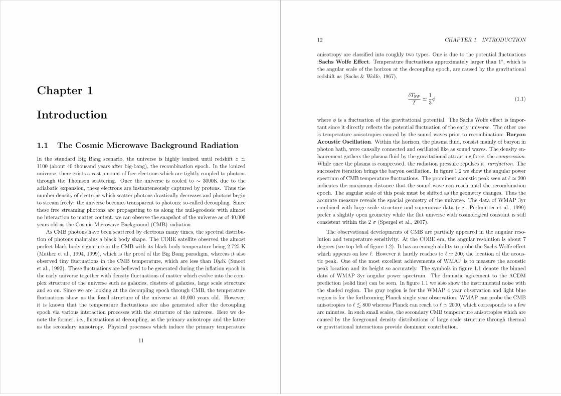
anisotropy are classified into roughly two types. One is due to the potential fluctuations
:Sachs Wolfe Effect. Temperature fluctuations approximately larger than 1, which isthe angular scale of the horizon at the decoupling epoch, are caused by the gravitational
redshift as (Sachs & Wolfe, 1967),
δTSWT
1
3φ (1.1)
where φ is a fluctuation of the gravitational potential. The Sachs Wolfe effect is impor-
tant since it directly reflects the potential fluctuation of the early universe. The other one
is temperature anisotropies caused by the sound waves prior to recombination: Baryon
Acoustic Oscillation. Within the horizon, the plasma fluid, consist mainly of baryon in
photon bath, were causally connected and oscillated like as sound waves. The density en-
hancement gathers the plasma fluid by the gravitational attracting force, the compression.
While once the plasma is compressed, the radiation pressure repulses it, rarefaction. The
successive iteration brings the baryon oscillation. In figure 1.2 we show the angular power
spectrum of CMB temperature fluctuations. The prominent acoustic peak seen at 200
indicates the maximum distance that the sound wave can reach until the recombination
epoch. The angular scale of this peak must be shifted as the geometry changes. Thus the
accurate measure reveals the spacial geometry of the universe. The data of WMAP 3yr
combined with large scale structure and supernovae data (e.g., Perlmutter et al., 1999)
prefer a slightly open geometry while the flat universe with cosmological constant is still
consistent within the 2 σ (Spergel et al., 2007).
The observational developments of CMB are partially appeared in the angular reso-
lution and temperature sensitivity. At the COBE era, the angular resolution is about 7
degrees (see top left of figure 1.2). It has an enough ability to probe the Sachs-Wolfe effect
which appears on low . However it hardly reaches to 200, the location of the acous-
tic peak. One of the most excellent achievements of WMAP is to measure the acoustic
peak location and its height so accurately. The symbols in figure 1.1 denote the binned
data of WMAP 3yr angular power spectrum. The dramatic agreement to the ΛCDM
prediction (solid line) can be seen. In figure 1.1 we also show the instrumental noise with
the shaded region. The gray region is for the WMAP 4 year observation and light blue
region is for the forthcoming Planck single year observation. WMAP can probe the CMB
anisotropies to 800 whereas Planck can reach to 2000, which corresponds to a few
arc minutes. In such small scales, the secondary CMB temperature anisotropies which are
caused by the foreground density distributions of large scale structure through thermal
or gravitational interactions provide dominant contribution.

1.1. THE COSMIC MICROWAVE BACKGROUND RADIATION 13
WMAP 3yr data
Figure 1.1: CMB Angular Power Spectrum for the temperature anisotropy. Symbols with error bars
are bin averaged WMAP 3yr data and solid blue line is best fit ΛCDM theoretical prediction. The gray
shaded region is expected 1 sigma error for WMAP 4 year observation and light blue shaded region is that
for PLANCK 1 year observation. Also plotted with black doted and solid lines are linear and non-linear
RS effect. On the largest scale, linear ISW is likely dominated the total CMB temperature fluctuations
while on small scales, the RS effect is less than primary by order of three.
θfwhm = 420 arcmin
θfwhm = 30 arcmin
θfwhm = 2 arcmin
Figure 1.2: Shown are simulated CMB temperature fluctuation maps for three angular resolutions with
420, 30 and 2 arcmin FWHM of the beam. These values are approximations of the COBE, WMAP
and ACT resolutions. The simulated maps are generated by synfast in Healpix ver 2.00 software with
Nside = 1024 (12,582,912 pixels) with same random seed.
14 CHAPTER 1. INTRODUCTION
1.2 CMB Secondary Anisotropies
After the photon-baryon decoupling, photons propagate along the null geodesic to us
through the large scale structure that lies at lower redshift than CMB. Since the large scale
structure has complex distributions of gravitational potentials and hot gases in the clusters
of galaxy that is neither isotropic nor homogeneous, the large scale structure imprints
the gravitational and/or thermal signatures on CMB temperature fluctuations. We thus
must observe the temperature fluctuation induced by the large scale structure, so-called
secondary CMB temperature anisotropies as well as those generated at the decoupling
epoch. Both the satellite such as PLANCK (Lamarre et al., 2003) and ground-based
observations such as Atacama Cosmological Telescope (ACT: Kosowsky, 2003) or South-
Pole Telescope (SPT Ruhl et al., 2004) will measure the CMB temperature fluctuations at
arc-minute scales (l > 1000) with sensitivities of ∼ µK, and thus are expected to detect
the secondary anisotropies. It is one of the major goals of the next generation CMB
experiments to separate each component of them.
The secondary anisotropies of CMB provide invaluable information on the history of
structure formation in the universe. Sources of the anisotropies include the thermal and
kinetic Sunyaev-Zeldovich (t/kSZ) effects by galaxy clusters and by patchy reionization,
the integrated Sachs-Wolfe (ISW) effect and its non-linear extension, the Rees-Sciama
(RS) effect, and the deflection effect of CMB by the gravitational lensing, with the relative
amplitudes at arc-minute scales being approximately less than the order of ∆T/T ∼ 10−5.The thermal SZ effect is induced by the hot gas of cluster of galaxies through the inverse-
compton scattering. As the hot gas modifies the photon distribution function from the
2.725K black-body distribution, the black-body temperature at long wave-length region
(Rayleigh-Jeans) decreases while it increases at short wave-length region (Wien). The
kinetic SZ effect is induced by electrons associated to bulk motions of clusters of galaxies
relative to the CMB rest frame.
The ISW effect is induced by the time variation of gravitational potentials of large
scale structure. As the CMB photon falls into the gravitational potentials, it gains the
energy while as the photon climbs up the potentials, it loses the energy. If the height of
gravitational potentials vary with time, the net energy chage would be expected. The RS
effect is induced by same mechanism. We use the term ISW when the underlying matter
density fluctuations of large scale structure are well described by the linear theory, while
the term RS is used when they need a non-linear treatment.
The Rees-Sciama effect, which is a main topic in this thesis, is, in principle, a unique
probe of the time-variation of gravitational potential, and thus provides information of
the rate of growth of large-scale structure on small scales (Rees & Sciama, 1968). In
addition the Rees-Sciama effect also occurres when a galaxy or a cluster of galaxies moves
1.3. OVERVIEW OF THE THESIS 15
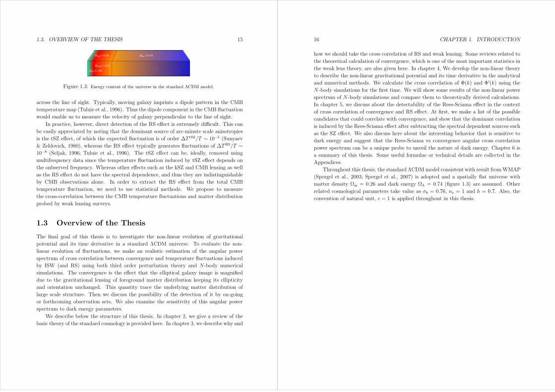
ΩΛ0 = 0.74ΩM0 = 0.26
Ωb0 = 0.04
ΩDM0 = 0.22
Figure 1.3: Energy content of the universe in the standard ΛCDM model.
across the line of sight. Typically, moving galaxy imprints a dipole pattern in the CMB
temperature map (Tuluie et al., 1996). Thus the dipole component in the CMB fluctuation
would enable us to measure the velocity of galaxy perpendicular to the line of sight.
In practice, however, direct detection of the RS effect is extremely difficult. This can
be easily appreciated by noting that the dominant source of arc-minute scale anisotropies
is the tSZ effect, of which the expected fluctuation is of order ∆T tSZ/T ∼ 10−5 (Sunyaev& Zeldovich, 1980), whereas the RS effect typically generates fluctuations of ∆TRS/T ∼10−8 (Seljak, 1996; Tuluie et al., 1996). The tSZ effect can be, ideally, removed usingmultifrequency data since the temperature fluctuation induced by tSZ effect depends on
the onbserved frequency. Whereas other effects such as the kSZ and CMB lensing as well
as the RS effect do not have the spectral dependence, and thus they are indistinguishable
by CMB observations alone. In order to extract the RS effect from the total CMB
temperature fluctuation, we need to use statistical methods. We propose to measure
the cross-correlation between the CMB temperature fluctuations and matter distribution
probed by weak lensing surveys.
1.3 Overview of the Thesis
The final goal of this thesis is to investigate the non-linear evolution of gravitational
potential and its time derivative in a standard ΛCDM universe. To evaluate the non-
linear evolution of fluctuations, we make an realistic estimation of the angular power
spectrum of cross correlation between convergence and temperature fluctuations induced
by ISW (and RS) using both third order perturbation theory and N -body numerical
simulations. The convergence is the effect that the elliptical galaxy image is magnified
due to the gravitational lensing of foreground matter distribution keeping its ellipticity
and orientation unchanged. This quantity trace the underlying matter distribution of
large scale structure. Then we discuss the possibility of the detection of it by on-going
or forthcoming observation sets. We also examine the sensitivity of this angular power
spectrum to dark energy parameters.
We describe below the structure of this thesis. In chapter 2, we give a review of the
basic theory of the standard cosmology is provided here. In chapter 3, we describe why and
16 CHAPTER 1. INTRODUCTION
how we should take the cross correlation of RS and weak lensing. Some reviews related to
the theoretical calculation of convergence, which is one of the most important statistics in
the weak lens theory, are also given here. In chapter 4, We develop the non-linear theory
to describe the non-linear gravitational potential and its time derivative in the analytical
and numerical methods. We calculate the cross correlation of Φ(k) and Φ′(k) using theN -body simulations for the first time. We will show some results of the non-linear power
spectrum of N -body simulations and compare them to theoretically derived calculations.
In chapter 5, we discuss about the detectability of the Rees-Sciama effect in the context
of cross correlation of convergence and RS effect. At first, we make a list of the possible
candidates that could correlate with convergence, and show that the dominant correlation
is induced by the Rees-Sciama effect after subtracting the spectral dependent sources such
as the SZ effect. We also discuss here about the interesting behavior that is sensitive to
dark energy and suggest that the Rees-Sciama vs convergence angular cross correlation
power spectrum can be a unique probe to unveil the nature of dark energy. Chapter 6 is
a summary of this thesis. Some useful formulae or technical details are collected in the
Appendices.
Throughout this thesis, the standard ΛCDMmodel consistent with result fromWMAP
(Spergel et al., 2003; Spergel et al., 2007) is adopted and a spatially flat universe with
matter density Ωm = 0.26 and dark energy ΩΛ = 0.74 (figure 1.3) are assumed. Other
related cosmological parameters take value as σ8 = 0.76, ns = 1 and h = 0.7. Also, the
convention of natural unit, c = 1 is applied throughout in this thesis.
Chapter 2
The Standard Cosmological Model
Recent cosmological observations reveal a number of mysteries of our universe. The
observations include temperature fluctuations of Cosmic Microwave Background (CMB),
luminosity distance from supernovae or gamma ray bursts, the cluster abundance from
wide field and deep galaxy surveys, distorted shapes of galaxy images by gravitational
lensing, the signature of baryon acoustic oscillation in the galaxy correlation and the
CMB temperature fluctuations generated at the large scale structure of the universe. The
combination of these observations suggests that our universe is accelerated expanding
since roughly about 6 billion years ago, the redshift z 1. In the framework of standard
theory of general relativity, all the results of these observations suggest the existence of
unknown energy component in a stress-energy tensor, the Λ term.
In this chapter, we will give a review of the standard theory of cosmology based on
the general relativity.
2.1 Relativistic Cosmology
In the zero-th approximation the universe is uniform and isotropic; there are any special
points and directions in the universe, the Cosmological Principle. It can be translated
as the generalization of Copernicus Principle. The most general spacetime metric that
satisfies the Cosmological Principle is given by Robertson-Walker metric. It can be written
in the spherical polar coordinate as
ds2 = gµνdxµdxν (2.1)
= a2[−dτ 2 + dr2
1− kr2+ r2(dθ2 + sin2 θdφ2)], (2.2)
where a is a scale factor, which is in general normalized to unity at today, and τ is
conformal time, related to cosmic time as adτ = dt. K is spacial curvature, andK >,<,=
17
18 CHAPTER 2. THE STANDARD COSMOLOGICAL MODEL
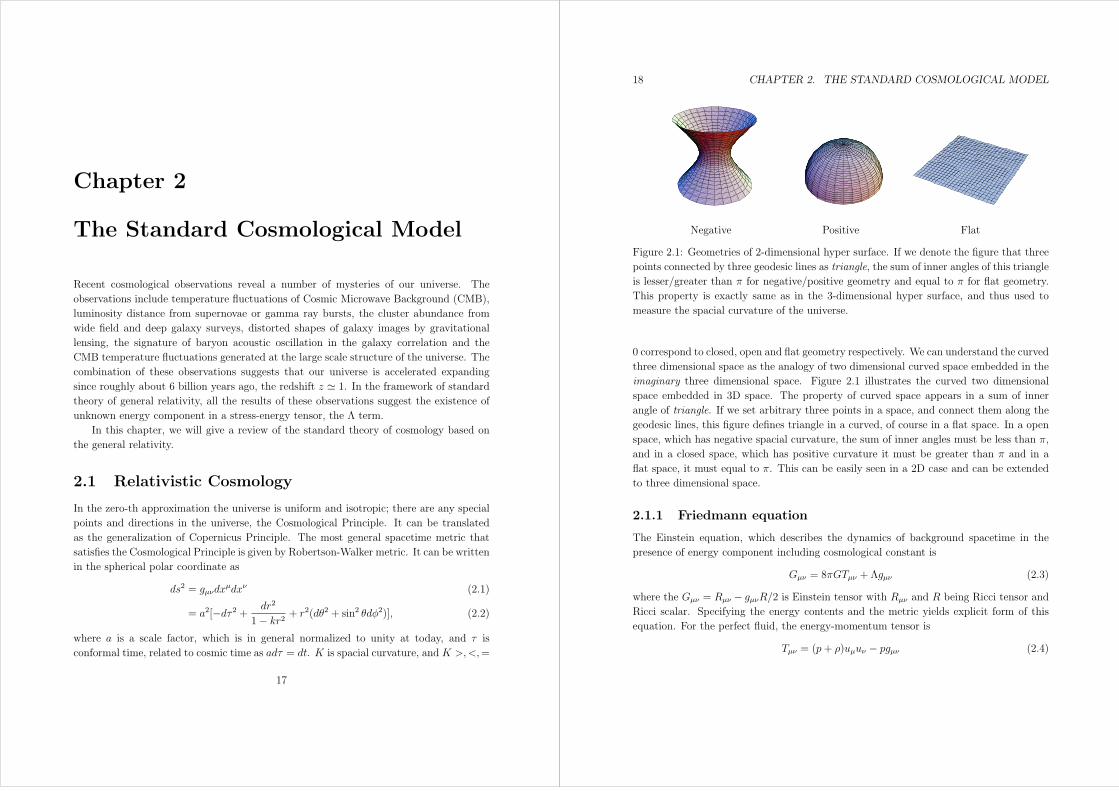
Negative Positive Flat
Figure 2.1: Geometries of 2-dimensional hyper surface. If we denote the figure that three
points connected by three geodesic lines as triangle, the sum of inner angles of this triangle
is lesser/greater than π for negative/positive geometry and equal to π for flat geometry.
This property is exactly same as in the 3-dimensional hyper surface, and thus used to
measure the spacial curvature of the universe.
0 correspond to closed, open and flat geometry respectively. We can understand the curved
three dimensional space as the analogy of two dimensional curved space embedded in the
imaginary three dimensional space. Figure 2.1 illustrates the curved two dimensional
space embedded in 3D space. The property of curved space appears in a sum of inner
angle of triangle. If we set arbitrary three points in a space, and connect them along the
geodesic lines, this figure defines triangle in a curved, of course in a flat space. In a open
space, which has negative spacial curvature, the sum of inner angles must be less than π,
and in a closed space, which has positive curvature it must be greater than π and in a
flat space, it must equal to π. This can be easily seen in a 2D case and can be extended
to three dimensional space.
2.1.1 Friedmann equation
The Einstein equation, which describes the dynamics of background spacetime in the
presence of energy component including cosmological constant is
Gµν = 8πGTµν + Λgµν (2.3)
where the Gµν = Rµν − gµνR/2 is Einstein tensor with Rµν and R being Ricci tensor and
Ricci scalar. Specifying the energy contents and the metric yields explicit form of this
equation. For the perfect fluid, the energy-momentum tensor is
Tµν = (p+ ρ)uµuν − pgµν (2.4)
2.1. RELATIVISTIC COSMOLOGY 19
where p is the pressure, ρ is the energy density and uµ is the fluid four velocity defined as
uµ = gµνdxν
ds(2.5)
In the universe described by Robertson-Walker metric, the Einstein equation yields(a
a
)2
=8πG
3ρ− K
a2+Λ
3(2.6)
a
a= −4πG
3(ρ+ 3p) +
Λ
3(2.7)
Equation (2.6) is 00 component of the Einstein equation and called as Friedmann equation
while the equation (2.7) is spacial part of equation (2.3), which is also derived from the
spacial part of energy conservation law, T µν;µ = 0. The Friedmann equation can be
rewritten as
H2(a) = H20 (Ωm0a
−3 + ΩK0a−2 + ΩΛ0) (2.8)
where H = a/a is Hubble parameter. Ωs are density parameters, which are normalized
by critical density, ρc0 = 3H20/8πG, and defined as
Ωm0 =8πGρ03H2
0
, ΩK0 = − K
H20
, ΩΛ0 =Λ
3H20
(2.9)
Note that the subscript 0 denotes the value of today and also that this notation of cur-
vature parameter is opposite in sign to usual definition. Now we introduce the equation
of state for each energy content that is defined as pressure to density ratio, w := p/ρ.
wm = 0 for a pressureless matter such as dark matter, wΛ = −1 for the cosmologicalconstant and wr = 1/3 for radiation such as photon. For the curvature, corresponding
equation of state is wK = −1/3. Then the Friedmann equation again rewritten as
H2(a) = H20
∑i
Ωi0Ei(a) (2.10)
I(a) = −H20
2
∑i
Ωi0Ei(a)[1 + 3wi(a)] (2.11)
Ei(a) = exp
[3
∫ 1
a
1 + wi(a′)
a′da′
](2.12)
where subscript i denotes the species of energy components and I(a) = a/a. Considering
the present epoch, following equation must be hold from equation (2.10),
1 = Ωm0 + Ωr0 + ΩΛ0 + ΩK0. (2.13)
20 CHAPTER 2. THE STANDARD COSMOLOGICAL MODEL
This relation must have equality for any time in the history of universe as
1 = Ωm + Ωr + ΩΛ + ΩK , (2.14)
with the density parameter at given time being
Ωi(a) = Ωi0Ei(a)H20
H2(a)(2.15)
2.1.2 Cosmological Distance
In an expanding universe, the distance can be defined in various manner. To this end,
it is convenient to introduce the idea of redshift. Suppose that the light is emitted with
wavelength λe, propagates to us along the null geodesic and is observed with λo. The
wavelength of light is elongated both due to the cosmological expansion and peculiar
motion of source against the observer, the Doppler shift. The redshift is defined as ratio
of two wavelength,
1 + z :=λoλe
(2.16)
In the absence of any peculiar motion, i.e. the emitting source is fixed on the comoving
frame, this exactly represents the expansion rate of universe thus
1 + z = a−1 (2.17)
is hold with normalization being a(t0) = 1
Comoving Distance
Imagine that the photon is emitted at (r, τ) = (r1, τ1), propagates along the null geodesic,
ds = 0 and is observed by us at (r, τ) = (0, t0). From the fact that the light propagates
isotropically, dθ = 0, dφ = 0. Then the metric given by equation (2.2) yeilds the relation,
dτ = − dr√1−Kr2
. (2.18)
Integrating along the line of sight gives the comoving distance, χ
χ =
∫ τ0
τ1
dτ =
∫ a0
a1
da
a2H(a)=
∫ z1
0
dz
H(z). (2.19)
In the second equality, dτ = dt/a = a/(aa2)da is used, and in the last equality, equation
(2.17) is used. The explicit relation between comoving distance and coordinate r is given
by integrating left hand side of equation (2.18). This yields immediately,
r =
sin(
√Kχ)/
√K, K > 0
χ, K = 0
sinh(√−Kχ)/
√−K, K < 0
(2.20)
2.1. RELATIVISTIC COSMOLOGY 21
Luminosity Distance
If one knows the luminosity of the light source, observed flux (or magnitude) can be a
measure of distance. Let me first consider the static Euclidean space. Imagine that the
light is emitted at (r, t) = (r1, t1) with luminosity L. The observed flux at (r, t) = (0, t0)
is reduced proportionally to distance squared,
f =L
4πr21(2.21)
The number of photons emitted between t1 and t1 + δt1 with frequency range between ν1and ν1 + δν1 is set to δN . The luminosity in this frequency band is then
δL = hν1δt1δN
(2.22)
Since the photon number must be conserved, the photon energy (flux) that passes through
the unit area perpendicular to the photon trajectory between t0 and t0+δt0 with frequency
range between ν0 and ν0 + δν0 is
δf =hν04πr2
δN
δt0. (2.23)
In a static Euclidean space, ν1 = ν0 and δt1 = δt0, while in an expanding spacetime
frequency and time interval are modified as ν1 = ν0(1 + z), δt1 = δt0/(1 + z). In an
expanding universe, equating δN of equations (2.22) and (2.23) and integrating over the
frequency yield
f =L
4πr2(1 + z)2(2.24)
Of course equating δN and integrating in a Euclidean space results in equation (2.21). If
we define luminosity distance as dL := r(1 + z) the expression is exactly same as that in
the Euclidean space (eq. (2.21))
f =L
4πd2L. (2.25)
Note that here f and L are bolometoric values. When the bolometoric information is not
available, one should have the K-correction. We do not mention to it in this thesis.
Angular Diameter Distance
22 CHAPTER 2. THE STANDARD COSMOLOGICAL MODEL
Again let me first consider the case for the Euclidean space. If there is a celestial object
whose size is known. Observing the subtended angle gives another measure of distance,
D = r∆θ, (2.26)
where D is size of the object perpendicular to the line of sight, ∆θ is its subtended angle
in the sky and r is distance to the object. In an expanding universe, integrating null
geodesic over the angle from right edge of the object to left edge equals to the physical
separation of the object, with dr = dφ = 0,
D =
∫ θL
θR
ar dθ = ar∆θ (2.27)
Compared with equation (2.26), if we define angular diameter distance as dA := r/(1+z),
the relation becomes same as Euclidean space.
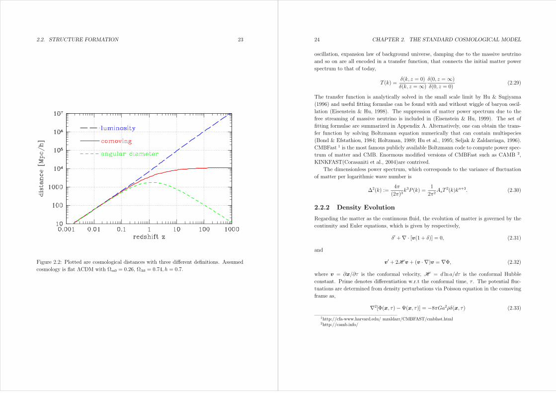
Figure 2.2 shows these three definitions of cosmological distance in standard ΛCDM
universe.
2.2 Structure formation
2.2.1 Primeval Density Fluctuations
In our universe, there are various structures that are bounded by gravitational force;
galaxy, cluster of galaxy and large-scale structure of the universe and so on. These
structure is thought to be constructed by the gravitational instability with the begining
of initial tiny fluctuations. The initial condition is given by power low matter power
spectrum as,
P (k) = Askn, (2.28)
where As is the amplitude of initial matter power spectrum and n is spectral index. If n =
1, initial matter power spectrum is scale invariant, or Zel’dovich spectrum. The WMAP
3yr data imposes the constraints on n and As as, n = 0.958 ± 0.016 and log(1010As) =
3.156± 0.056 (Spergel et al., 2007). This implies that the initial matter power spectrumalmost equals to scale invariant, but slightly deviate from it. So, the values of n and As
above are conventionally measured at k = 0.002h/Mpc.
The CDM density fluctuations that are smaller than horizon scale interact with other
species such as photon, baryon and neutrino. While the fluctuations that are larger than
Hubble radius does not interact with these species and conserve the information of initial
density fluctuations. The physical effects, including Silk damping, damping due to baryon
2.2. STRUCTURE FORMATION 23
Figure 2.2: Plotted are cosmological distances with three different definitions. Assumed
cosmology is flat ΛCDM with Ωm0 = 0.26, ΩΛ0 = 0.74, h = 0.7.
24 CHAPTER 2. THE STANDARD COSMOLOGICAL MODEL
oscillation, expansion law of background universe, damping due to the massive neutrino
and so on are all encoded in a transfer function, that connects the initial matter power
spectrum to that of today,
T (k) =δ(k, z = 0)
δ(k, z =∞)δ(0, z =∞)δ(0, z = 0)
(2.29)
The transfer function is analytically solved in the small scale limit by Hu & Sugiyama
(1996) and useful fitting formulae can be found with and without wiggle of baryon oscil-
lation (Eisenstein & Hu, 1998). The suppression of matter power spectrum due to the
free streaming of massive neutrino is included in (Eisenstein & Hu, 1999). The set of
fitting formulae are summarized in Appendix A. Alternatively, one can obtain the trans-
fer function by solving Boltzmann equation numerically that can contain multispecies
(Bond & Efstathiou, 1984; Holtzman, 1989; Hu et al., 1995; Seljak & Zaldarriaga, 1996).
CMBFast 1 is the most famous publicly available Boltzmann code to compute power spec-
trum of matter and CMB. Enormous modified versions of CMBFast such as CAMB 2,
KINKFAST(Corasaniti et al., 2004)are contrived.
The dimensionless power spectrum, which corresponds to the variance of fluctuation
of matter per logarithmic wave number is
∆2(k) :=4π
(2π)3k3P (k) =
1
2π2AsT
2(k)kn+3. (2.30)
2.2.2 Density Evolution
Regarding the matter as the continuous fluid, the evolution of matter is governed by the
continuity and Euler equations, which is given by respectively,
δ′ +∇ · [v(1 + δ)] = 0, (2.31)
and
v′ + 2H v + (v · ∇)v = ∇Φ, (2.32)
where v = ∂x/∂τ is the conformal velocity, H = d ln a/dτ is the conformal Hubble
constant. Prime denotes differentiation w.r.t the conformal time, τ . The potential fluc-
tuations are determined from density perturbations via Poisson equation in the comoving
frame as,
∇2[Φ(x, τ)−Ψ(x, τ)] = −8πGa2ρδ(x, τ) (2.33)
1http://cfa-www.harvard.edu/ mzaldarr/CMBFAST/cmbfast.html2http://camb.info/

2.2. STRUCTURE FORMATION 25
where Φ is Bardeen’s curvature perturbation during the matter-dominated era and related
to the trace of metric as gii = 3a2(1 + 2Φ), whereas Ψ is given by the g00 component,
g00 = −a2(1+2Ψ) (Kodama & Sasaki, 1984; Bardeen, 1980). In the absence of significant
sources of anisotropic stress, which is always the case, these two quantities are related to
each other by Φ = −Ψ.In the linear perturbation theory, the evolution of the density fluctuations does not
depend on scales so that the density fluctuations can be factorized as δ(x, τ) = D(τ)δ(x),
where δ(x) is the initial density fluctuation. Then combining equations (2.31)-(2.33)
yields the evolution equation for the matter,
D′′ + 2H D′ +3
2Ωm0H
20 D = 0. (2.34)
Since this equation is second order differential equation, it has two special solutions,
growing mode and decaying mode. However the magnitude of decaying mode decrease
rapidly thus we can ignore the contribution from decaying mode. In the matter-dominated
era, the solution D(a) is given by the scale factor, a (e.g., Peacock, 1999) and one can use
the fitting formula in the ΛCDM case(Carroll et al., 1992) when 0.03 ≤ ΩM ≤ 2,−5 ≤ΩΛ ≤ 5. For general case, equation (2.34) can be integrated numerically to obtain the
linear growth factor. To this end, it is convenient to rewrite equation (2.34) as (Matsubara
& Szalay, 2003)
f =d lnD
d ln a, (2.35)
d f
d ln a= −f 2 − (1− d lnH
d ln a)f +
3
2ΩM(a) (2.36)
Here f is the growth factor of the linear velocity field.
It is convenient to work with the Fourier transforms of the above equations: For
continuity equation,
δ′(k) = −iθ(k)− i
∫d3q
(2π)3δ(k − q)θ(q)
k · qq2
(2.37)
where θ is divergence of velocity, k · v. For Poisson equation,
k2Φ(k) =3ΩmH
20
2
δ(k)
a. (2.38)
Figure 2.3 shows growth factor of linear density fluctuations, the solution of equation
(2.34) (left) and that of linear velocity field given by equation (2.35) (right). Since the
linear growth rate is normalized to unity at present, shift from EdS case to the upper
side at past time means larger amplitude of initial density fluctuations than EdS. In other
26 CHAPTER 2. THE STANDARD COSMOLOGICAL MODEL
0.01 0.1 1 10 1000
0.2
0.4
0.6
0.8
1
redshit z0.01 0.1 1 10 1000
0.2
0.4
0.6
0.8
1
redshit z
EdS
Figure 2.3: (Left) Plotted are growth factor of linear density fluctuation normalized to
unity at present epoch. The solid(black) and long-dashed(green) lines are ΛCDM model
with ΩΛ0 = 0.74, 0.5 respectively. The short-dashed(red) and dashed-dotted(blue) lines
are QCDMmodel, which means energy density of dark energy is not constant, equivalently
w = −1, with ΩΛ0 = 0.74, 0.5 respectively. We assume w = −1/3 for latter two QCDMmodels. Also plotted with thin dotted(cyan) line corresponds to EdS case in which the
D is proportional to scale factor a. (Right) Plotted are growth of linear velocity field,
f = d lnD/d ln a. All lines describe same models as left panel.
2.3. STATISTICS OF LARGE-SCALE-STRUCTURE 27
words, the larger initial fluctuations are required to realize today’s amplitude of density
fluctuations because the growth suppression should be occurred due to the dark energy.
The effect of dark energy appears more prominently in the velocity field (right panel of
figure 2.3). For the EdS universe, f is always unity. Dark energy also works to suppress
the evolution of velocity field. The amplitude of suppression at present epoch is sensitive
to the present value of dark energy while the epoch of deviation from EdS depends largely
on the equation of state. This can be explained that the larger value of equation of state
makes the dark energy significant at earlier time.
2.3 Statistics of Large-Scale-Structure
2.3.1 Gaussian Random Field
If the field is a random Gaussian, all the statistical properties can be described by second
order statistics, e.g., the quadratic quantities of the field such as the power spectrum and
the two point correlation function (2PCF). The density fluctuation is defined by
δ(x) :=ρ(x)− ρ
ρ, (2.39)
where the ρ(x) is the density at position x and ρ denotes the averaged density over the
whole universe at same epoch. The Fourier coefficients of density fluctuation in a volume
V , δ(x) is in general complex number
δk = Re δk + iIm δk = |δk|eiθk , (2.40)
i.e. the amplitude |δk| and phase θk. The reality of δ(x) constraints the condition on δk
as
δ∗k = δ−k (2.41)
The term, random Gaussian field, means that the phase of δk is random, or not correlated
and the probability of real and imaginary part of δk obeys Gaussian distribution function,
P(w) =√
V
2πσ2kexp
[−w2V
2σ2k
](2.42)
where the variance σ2k = δ2k/2. Thus the probability distribution function of moduli
becomes Rayleigh distribution,
P(|δk|, θk) d|δk| dθk =|δk|V2πδ2k
exp
[−|δk|
2V
2δ2k
]d|δk| dθk (2.43)
28 CHAPTER 2. THE STANDARD COSMOLOGICAL MODEL
If the Fourier quantity |δk| obeys this Rayleigh distribution, real space density field δ(x)
has Gaussian distribution,
P(δ) dδ = 1√2πσ2
exp
[− δ2
2σ2
]dδ (2.44)
2.3.2 Power Spectrum and 2PCF
As can be seen from the previous section, the density fluctuations take various values:
density in some place is larger than average and smaller in other place. Thus in the
cosmological context, the values of density fluctuations themselves have no meaningful
information. Then the statistical treatment enables us to extract invaluable information
about the cosmology. By the definition of density fluctuation, the expectation value of δ
must be vanish,
〈δ(x)〉 = 0 (2.45)
We now focus on the arbitrary one position x1 in which the density fluctuation is δ1and measure the density fluctuation around there with position x2. Let it denotes δ2. If
the universe is perfectly isotropic and homogeneous, δ1 and δ2 is identical independent
from the selection of position : there are no correlations between δ1 and δ2. Even in the
inhomogeneous and anisotropic universe, if the separation of two positions is infinitely
large then statistically δ1 and δ2 can not be thought to have a correlation. In the finite
separation, there must be correlation between two due to the clustering induced by gravi-
tational interaction or other physical effects. Thus the product of two density fluctuations
with the separation being x1 − x2 averaged over the universe must have an cosmological
information, the clustering, or the degree of localized concentration of the field. (see e.g.,
Peebles, 1980)
These intuitions are quantified by the 2PCF, defined as
〈δ(x1) δ(x2)〉 := ξ(x12), (2.46)
where x12 = |x2−x1| is the distance between x1 and x2. Since the universe is statistically
isotropic, correlation function does not depend on the angle. In addition since the universe
is statistically homogeneous, it also does not depend on the position but only on the
separation of two points. Such a statistical treatment can be performed also in the Fourier
space. The Fourier counterpart of density fluctuation is
δ(k) =
∫d3x δ(x)e−ik·x (2.47)
2.3. STATISTICS OF LARGE-SCALE-STRUCTURE 29
The ensemble average of δ(k) can be calculated as
〈δ(k) δ∗(k′)〉 =∫∫
d3x1d3x2 〈δ(x1) δ(x2)〉 e−i(k·x1−k′·x2) (2.48a)
=
∫∫d3x1d
3x12 ξ(x12)e−i(k−k′)·x1+ik
′·x12 (2.48b)
= (2π)3δD(k − k′)∫
d3x12 ξ(x12)eik′·x12 (2.48c)
= (2π)3δD(k − k′)∫
x2dx4π sin(kx)
kxξ(x) (2.48d)
Thus if we define the power spectrum as
〈δ(k)δ∗(k′)〉 := (2π)3δD(k − k′)P (k), (2.49)
then the well known Wiener-Khintchine relation is obtained. Again from the statistical
isotropy, the power spectrum does not depend on the angles of wave number vectors but
only on the modulus of them.
The cross correlation of two kinds of field, δa, δb can be defined in the same manner,
ξab(x) = 〈δa(x′) δb(x+ x′)〉 (2.50)
Pab(k) = (2π)3δD(k − k′) 〈δa(k′) δb(k′)〉 (2.51)
estimation of power spectrum
In order to evaluate three dimensional correlation function or power spectrum, the
information of three dimensional position is required. For us, it is easy to measure the 2
dimensional angular position in the celestial sphere however the radial information is hard
to obtain since we are fixed at the origin of spherical coordinate. Though we have various
measures to determine the radial distance appropriate for its distance: annual parallax
method, variable star method for the distance to neighborhood objects or measurement
of redshift for cosmologically distant objects. For galaxies with cosmological distance,
identification of radial positions always requires the measurement of redshift. Since the
measurement of redshift requires spectroscopic observation of object, which is in general
difficult, it should be challenging to measure a three dimensional correlation function or
power spectrum.
Recent large spectroscopic galaxy survey such as 2 degree Field Galaxy Redshift
Survey (2dFGRS) or Sloan Digital Sky Survey (SDSS) measures the three dimensional
matter power spectrum using the spectroscopic observation of galaxies. For 2dF, the 3D
power spectrum is measured for galaxies (Peacock, 2001; Percival et al., 2001; Tegmark
et al., 2002; Percival, 2005; Cole et al., 2005) in a complementary way, and for the QSO
30 CHAPTER 2. THE STANDARD COSMOLOGICAL MODEL
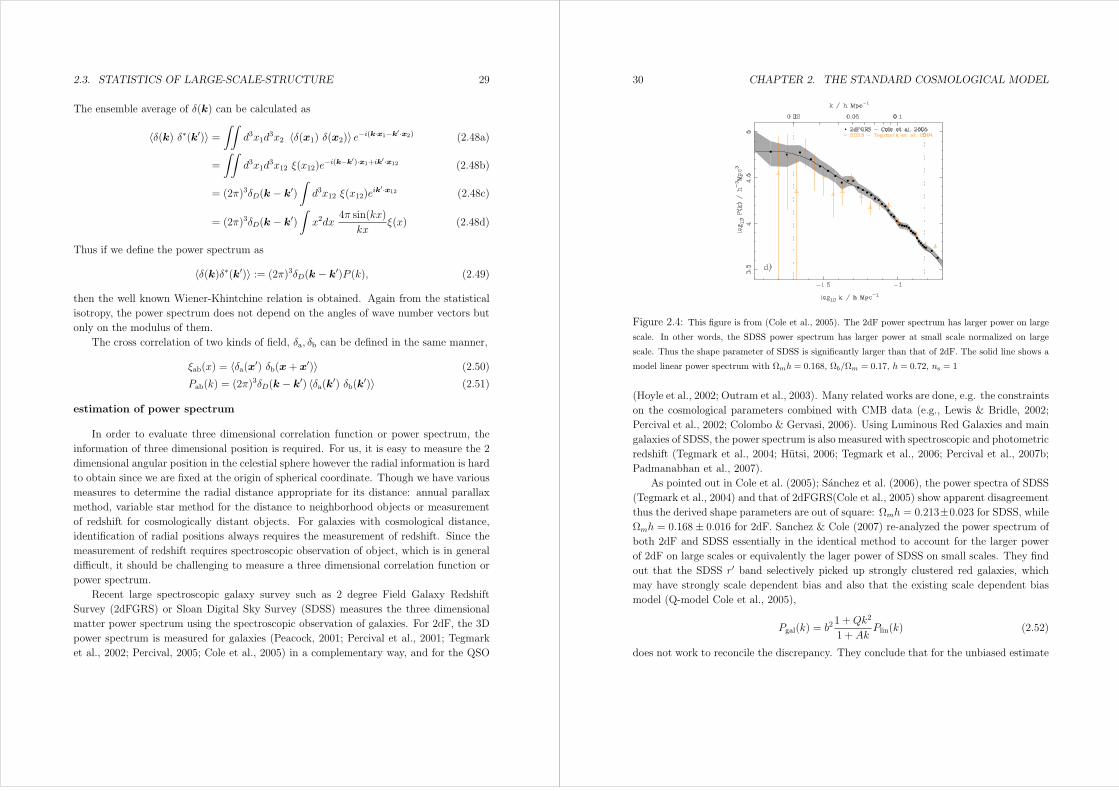
Figure 2.4: This figure is from (Cole et al., 2005). The 2dF power spectrum has larger power on large
scale. In other words, the SDSS power spectrum has larger power at small scale normalized on large
scale. Thus the shape parameter of SDSS is significantly larger than that of 2dF. The solid line shows a
model linear power spectrum with Ωmh = 0.168, Ωb/Ωm = 0.17, h = 0.72, ns = 1
(Hoyle et al., 2002; Outram et al., 2003). Many related works are done, e.g. the constraints
on the cosmological parameters combined with CMB data (e.g., Lewis & Bridle, 2002;
Percival et al., 2002; Colombo & Gervasi, 2006). Using Luminous Red Galaxies and main
galaxies of SDSS, the power spectrum is also measured with spectroscopic and photometric
redshift (Tegmark et al., 2004; Hutsi, 2006; Tegmark et al., 2006; Percival et al., 2007b;
Padmanabhan et al., 2007).
As pointed out in Cole et al. (2005); Sanchez et al. (2006), the power spectra of SDSS
(Tegmark et al., 2004) and that of 2dFGRS(Cole et al., 2005) show apparent disagreement
thus the derived shape parameters are out of square: Ωmh = 0.213±0.023 for SDSS, whileΩmh = 0.168± 0.016 for 2dF. Sanchez & Cole (2007) re-analyzed the power spectrum of
both 2dF and SDSS essentially in the identical method to account for the larger power
of 2dF on large scales or equivalently the lager power of SDSS on small scales. They find
out that the SDSS r′ band selectively picked up strongly clustered red galaxies, whichmay have strongly scale dependent bias and also that the existing scale dependent bias
model (Q-model Cole et al., 2005),
Pgal(k) = b21 +Qk2
1 + AkPlin(k) (2.52)
does not work to reconcile the discrepancy. They conclude that for the unbiased estimate
2.3. STATISTICS OF LARGE-SCALE-STRUCTURE 31
of cosmological parameters, the better understandings about the physical or at least
empirical processes which shape the power spectrum are desired.
2.3.3 Angular Power Spectrum
An angular correlation is useful when we can not obtain accurate measurement of radial
distances to the objects or when it is essentially unavailable. For example, the galaxy
distribution with poor measure of redshift is projected to the celestial sphere with appro-
priately forecasted radial selection function should be measured with angular function.
As an another example, intrinsically CMB temperature fluctuations are projected photon
distribution at the last scattering surface thus we need to measure them with the angular
function.
Any functions f(θ, φ) defined on the sphere can be expanded on the basis of the
spherical harmonics (Laplace’s series).
f(n) =∑,m
amYm(n), (2.53)
The unit direction vector n is set to point the orientation of (θ, φ) thus the angular
dependency can be replaced by n. If f is known, the coefficient am can be immediately
found by the orthogonality integral,
am =
∫dΩ f(n)Ym(n), (2.54)
where dΩ = sin2 θdθdφ is the solid angle element. Note that the sum of equation (2.53)
runs over −(+1) ≤ m ≤ +1 and 0 ≤ ≤ ∞ for the mathematical definition. Practically
the monopole, = 0, determines the overall amplitude and does not contribute to the
anisotropies. The angular power spectrum is defined as
〈ama∗′m′〉 = C δ′δmm′ (2.55)
Consider that the function on the sphere is a consequence of the projection of the field
which actually has three dimensional distribution in the universe. It can be represented
by the line of sight integral with appropriate weight kernel,
f(n) =
∫ rH
0
dr W (r)F (nr), (2.56)
where F is any field defined in a 3-dimensional hyper-surface, and W is the radial weight.
Fourier transforming F and expanding plane wave in a series of spherical wave (Rayleigh
32 CHAPTER 2. THE STANDARD COSMOLOGICAL MODEL
expansion) yields
F (nr) = 4π∑m
(−i)∫
d3k
(2π)3F (k)j(kr)Ym(k)Ym(n)
∗ (2.57)
Thus the angular power spectrum of any combination of two fields is calculated as
δ′δmm′Cab = (4π)2
∑λµ
∑λ′µ′
∫∫dΩ1dΩ2
∫∫dr1dr2
∫∫d3k1(2π)3
d3k2(2π)3
×Wa(r1)Wb(r2)⟨Fa(k1)F
∗b (k2)
⟩jλ(k1r1)jλ′(k2r2)
× Ym(n1)Y∗′m′(n2)Yλµ(k1)Y
∗λ′µ′(k2)Y
∗λµ(n1)Yλ′µ′(n2) (2.58a)
= (4π)2∫∫
dr1dr2
∫∫d3k1(2π)3
d3k2(2π)3
×Wa(r1)Wb(r2)(2π)3δD(k1 − k2)Pab(k1)j(k1r1)j′(k2r2)
× Ym(k1)Y∗′m′(k2) (2.58b)
= (4π)2∫∫
dr1dr2
∫d3k
(2π)3
×Wa(r1)Wb(r2)Pab(k)j(kr1)j′(kr2)Ym(k)Y∗′m′(k) (2.58c)
= δmδ′m′8π
∫∫dr1dr2
∫k2dk Wa(r1)Wb(r2)Pab(k)j(kr1)j′(kr2) (2.58d)
For the multipoles larger than 10 , which roughly corresponds to angular scale of 20
degree, the small angle approximation or flat sky approximation can be applied (Limber,
1954; Peebles, 1980; Afshordi et al., 2004) since the spherical Bessel function picks up the
mode at scale kr. Thus the spherical Bessel function can be replaced by Dirac delta
function as
j(kr) √
π
2+ 1
[δD
−
(kr − 1
2
)+O(−2)
]. (2.59)
Application of this approximation extremely advances the performance of calculation
time because the multiple integral of equation (2.58d) is replaced with the integrand in
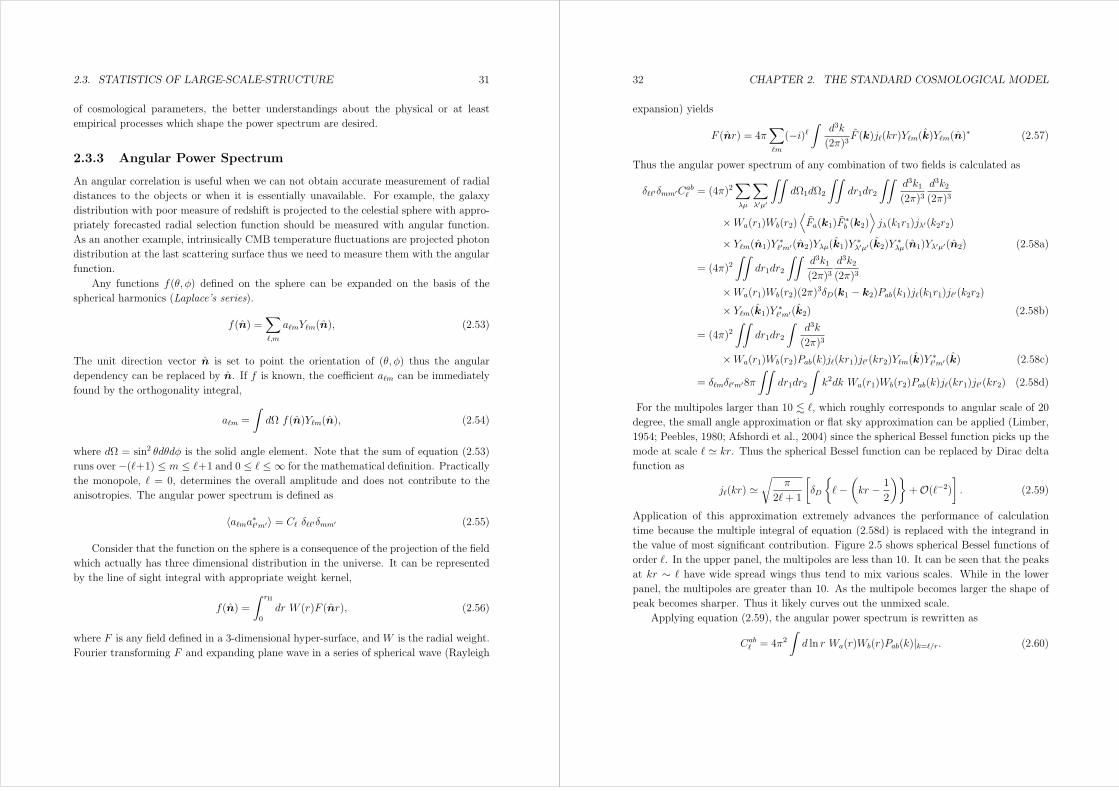
the value of most significant contribution. Figure 2.5 shows spherical Bessel functions of
order . In the upper panel, the multipoles are less than 10. It can be seen that the peaks
at kr ∼ have wide spread wings thus tend to mix various scales. While in the lower
panel, the multipoles are greater than 10. As the multipole becomes larger the shape of
peak becomes sharper. Thus it likely curves out the unmixed scale.
Applying equation (2.59), the angular power spectrum is rewritten as
Cab = 4π2
∫d ln r Wa(r)Wb(r)Pab(k)|k=/r. (2.60)
2.3. STATISTICS OF LARGE-SCALE-STRUCTURE 33
Figure 2.5: Shown are spherical Bessel functions. In the upper panel, the multipoles are
less than 10. It can be seen that the peaks at kr ∼ has wide spread wing thus tends
to mix various scale. While in the lower panel, the multipoles are grater than 10. As
the multipole become larger the shape of peak becomes sharper. Thus it curves out the
unmixed scale.
34 CHAPTER 2. THE STANDARD COSMOLOGICAL MODEL
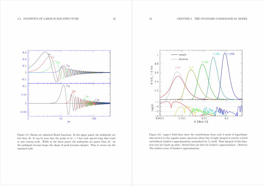
Figure 2.6: (upper) Solid lines show the contributions from each k mode of logarithmic
interval ln k to the angular power spectrum whose line of sight integral is exactly carried
out(without Limber’s approximation) normalized by C itself. Thus integral of this func-
tion over ln k lands up unity. Dotted lines are that for Limber’s approximation. (Bottom)
The relative error of Limber’s approximation.
2.3. STATISTICS OF LARGE-SCALE-STRUCTURE 35
multipole l
l(l+
1)C
l /
2π
∆
ΩΛ = 0.74
Ωm = 0.26
h = 0.7
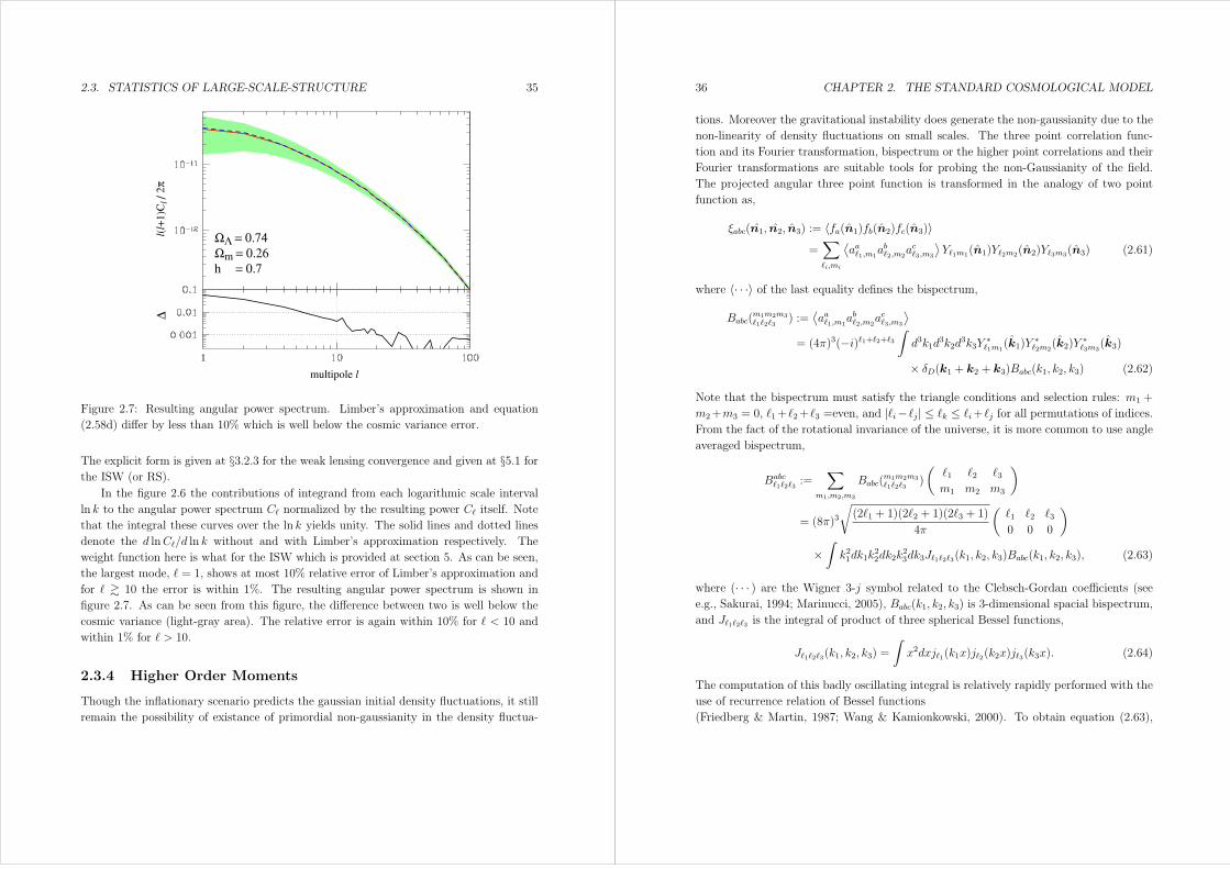
Figure 2.7: Resulting angular power spectrum. Limber’s approximation and equation
(2.58d) differ by less than 10% which is well below the cosmic variance error.
The explicit form is given at §3.2.3 for the weak lensing convergence and given at §5.1 forthe ISW (or RS).
In the figure 2.6 the contributions of integrand from each logarithmic scale interval
ln k to the angular power spectrum C normalized by the resulting power C itself. Note
that the integral these curves over the ln k yields unity. The solid lines and dotted lines
denote the d lnC/d ln k without and with Limber’s approximation respectively. The
weight function here is what for the ISW which is provided at section 5. As can be seen,
the largest mode, = 1, shows at most 10% relative error of Limber’s approximation and
for 10 the error is within 1%. The resulting angular power spectrum is shown in
figure 2.7. As can be seen from this figure, the difference between two is well below the
cosmic variance (light-gray area). The relative error is again within 10% for < 10 and
within 1% for > 10.
2.3.4 Higher Order Moments
Though the inflationary scenario predicts the gaussian initial density fluctuations, it still
remain the possibility of existance of primordial non-gaussianity in the density fluctua-
36 CHAPTER 2. THE STANDARD COSMOLOGICAL MODEL
tions. Moreover the gravitational instability does generate the non-gaussianity due to the
non-linearity of density fluctuations on small scales. The three point correlation func-
tion and its Fourier transformation, bispectrum or the higher point correlations and their
Fourier transformations are suitable tools for probing the non-Gaussianity of the field.
The projected angular three point function is transformed in the analogy of two point
function as,
ξabc(n1, n2, n3) := 〈fa(n1)fb(n2)fc(n3)〉=
∑i,mi
⟨aa1,m1
ab2,m2ac3,m3
⟩Y1m1(n1)Y2m2(n2)Y3m3(n3) (2.61)
where 〈· · ·〉 of the last equality defines the bispectrum,
Babc(m1m2m3123
) :=⟨aa1,m1
ab2,m2ac3,m3
⟩= (4π)3(−i)1+2+3
∫d3k1d
3k2d3k3Y
∗1m1
(k1)Y∗2m2
(k2)Y∗3m3
(k3)
× δD(k1 + k2 + k3)Babc(k1, k2, k3) (2.62)
Note that the bispectrum must satisfy the triangle conditions and selection rules: m1 +
m2+m3 = 0, 1+ 2+ 3 =even, and |i− j| ≤ k ≤ i+ j for all permutations of indices.
From the fact of the rotational invariance of the universe, it is more common to use angle
averaged bispectrum,
Babc123
:=∑
m1,m2,m3
Babc(m1m2m3123
)
(1 2 3m1 m2 m3
)
= (8π)3√(21 + 1)(22 + 1)(23 + 1)
4π
(1 2 30 0 0
)
×∫
k21dk1k22dk2k
23dk3J123(k1, k2, k3)Babc(k1, k2, k3), (2.63)
where (· · · ) are the Wigner 3-j symbol related to the Clebsch-Gordan coefficients (seee.g., Sakurai, 1994; Marinucci, 2005), Babc(k1, k2, k3) is 3-dimensional spacial bispectrum,
and J123 is the integral of product of three spherical Bessel functions,
J123(k1, k2, k3) =
∫x2dxj1(k1x)j2(k2x)j3(k3x). (2.64)
The computation of this badly oscillating integral is relatively rapidly performed with the
use of recurrence relation of Bessel functions
(Friedberg & Martin, 1987; Wang & Kamionkowski, 2000). To obtain equation (2.63),
2.3. STATISTICS OF LARGE-SCALE-STRUCTURE 37
the Gaunt integral,
Gm1m2m3123
:=
∫dΩY1m1Y2m2Y3m3
=
√(21 + 1)(22 + 1)(23 + 1)
4π
(1 2 30 0 0
)(1 2 3m1 m2 m3
)(2.65)
and the identity
∑m1,m2,m3
(1 2 3m1 m2 m3
)Gm1m2m3123
=
√(21 + 1)(22 + 1)(23 + 1)
4π
(1 2 30 0 0
)
(2.66)
are used. The reduced bispectrum is used in the literature(Komatsu & Spergel, 2001),
which contains all the physical information in the bispectrum,
b123 := Babc123
√4π
(21 + 1)(22 + 1)(23 + 1)
(1 2 30 0 0
)−1(2.67)
or similar quantity to this can be found as Bl1l2l3 in (Magueijo, 2000).
38 CHAPTER 2. THE STANDARD COSMOLOGICAL MODEL
Chapter 3
Observational Probes
3.1 The Rees-Sciama Effect
The Rees-Sciama Effect is one of the mechanisms that generates the temperature fluctu-
ations of the CMB. Most of the temperature fluctuations are generated at the decoupling
epoch, z 1100 however on small scales, they could arise from the inhomogeneous dis-
tribution of foreground large scale structure (LSS). The RS effect brings temperature
fluctuations due to the time variation of the gravitational potential of the large scale
structure, which is induced on large scales by an accelerating expansion due to dark en-
ergy and on small scales by a gravitational collapse of bounded objects, such as clusters
of galaxy. When the CMB photon falls into the gravitational potential of LSS, it gains
the energy, or blueshifts. Whereas when it climbs up the potential well, it loses its en-
ergy, or redshifts. If the potential would not vary with time during the photon passage,
the amount of blueshift and redshift is balanced and the net effects are cancelled out.
However, since the potential in general evolves with time, the net energy gain or loss is
expected.
In the flat universe, temperature fluctuations induced by the RS effect can be ex-
pressed by the line of sight integral of time derivative of gravitational potential,
∆TRST
(n) = −2∫
dr∂Φ(nr; r)
∂r(3.1)
Readers should refer to the Appendix C for the derivation. Below an arcmin scale, this
brings the temperature fluctuations of order ∆TRS/T ∼ 10−8 (Seljak, 1996; Tuluie et al.,1996), which is smaller than that of primary CMB or that of thermal Sunyaev Zel’dovich
effect by order of magnitude three.
The CMB temperature fluctuations we observe are the total fluctuations including
primary fluctuations at decoupling epoch, thermal/kinetic SZ, RS and so on. Thus it is
39
40 CHAPTER 3. OBSERVATIONAL PROBES
likely impossible to isolate the temperature fluctuations generated by the RS effect from
the total CMB temperature fluctuations. We show here only the conceptual idea and will
give a detail in section 5.
3.1.1 Why using Cross Correlation ?
Now our goal is the detachment of the tiny fluctuations of RS effect in the total CMB
temperature fluctuations. As we mentioned above, the RS effect is smaller than other
sources of fluctuations by order of three. We propose to use the statistical method, the
cross correlation. Because the RS effect is generated by the large scale structure, it must
correlate with the matter distribution of LSS. The candidates of quantity that measures
the matter distribution could be the galaxy distribution and statistics of weak lensing. Of
which, the galaxy distribution has crucial disadvantage, the galaxy bias problem. The nat-
ural interpretation of CDM structure formation theory claims that the galaxies are born
at high density regions of the underlying dark matter. Thus the simplest consideration
results in the so called linear bias,
δgal = bδdm (3.2)
i.e. the density contrast of galaxy is proportional to that of dark matter. This idea
is acceptable on large scales however on small scales, where the density contrast is not
so small, δ 1, this relation must no more valid and any predictions of the galaxy
bias do not have the universality, it depends largely on the survey thus on the galaxy
population. Therefore the galaxy distribution is not a reliable or robust tracer for the
matter distribution. Whereas the convergence of weak lensing never suffer from the bias
problem. The convergence is one of the statistics which we explain later in this chapter.
It probes the mass lying between the lensed galaxy and us along the line of sight. Working
in the harmonic space, the observable quantity is the Cross Correlation Angular Power
Spectrum (CCAPS) between the RS and convergence. The expression of CCAPS is
written as
CRS−κ = −22
∫dzs n(zs)
∫ rs
0
drrs − r
r3rsPΦΦ′(k; r)|k=/r (3.3)
Thus for the theoretical prediction of CCAPS, PΦΦ′ , the power spectrum of gravitational
potential and its time derivative, is required. It can be rewritten as
PΦΦ′(k, τ) =
(3
2
Ωm0H20
ak2
)2
[Pδδ′(k, τ)−H Pδδ(k, τ)] . (3.4)

3.2. WEAK GRAVITATIONAL LENSING 41
It is straightforward to calculate this power spectrum within the linear regime since δ′(z) =D′(z)δ(0) = fH δ(z), thus
P linΦΦ′(k, z) =
(3
2
Ωm0
a
H20
k2
)2
[H (z)f(z)− 1]P linδδ (k, z). (3.5)
However we need the CCAPS below the arcmin scale where the power spectrum requires
the non-linear treatment. This is a main problem in this thesis to estimate the CCAPS
on these scales. We tried to evaluate CCAPS in both analytical and numerical manner.
The details of these treatments can be found in the section 4.
The rest of this chapter is devoted to develop the weak lensing theory and statistical
treatment.
3.2 Weak Gravitational Lensing
The light bundle emitted at source object travels along the geodesic line of space time.
Since the geometry around the gravitationally bounded object is locally curved, the pho-
ton path near the object seems to be bent. As can be seen below, since the gravitational
lens is sensitive both to angular diameter distance and density growth, the lens system
with cosmological distance can be used to measure the cosmological information.
Figure 3.1 shows an example of strong lensing event 1. Four multiple images are
clearly appeared. And one can also see the large arc between image A2 and B. For
the weak lensing there never appears such a giant arc or multiple images but just exists
slight distortion in their images or ellipticities. Because in general, the strong lensing
occur only when the location of lens and source is very close in the 2 dimensional sky, the
probability of strong lensing event is small. While for the weak lens, since the light should
be deflected more or less by the large scale structure of the universe during propagation
and its impact parameter must be large, the probability of weak lens event is enormous. In
other words, all of the light we observe is lensed, and distorted at least the inhomogeneous
structures of the universe, the cosmic shear. Figure 3.2 shows Abell 1689 cluster, one of
the predominant examples of the gravitational lens event. This image is taken by Hubble
Space Telescope with Advanced Camera of Survey. The lensed galaxy images are faint
and elongated along the direction tangential to the circle centered at cluster center.
1Images are available at CASTLE : http://cfa-www.harvard.edu/glensdata/
42 CHAPTER 3. OBSERVATIONAL PROBES
Figure 3.1: An example of strong lens : MG J0414+0534. Source object is quasar at
z = 2.64 and lens is early type galaxy at z = 0.96. This figure is taken by Green Bank
Telescope and cited from Curran et al. (2007). The data of lens systems including this
figure is available at CASTLE
3.2.1 Light Deflection
set up
The situation considered here is summarized in figure 3.3. The mass concentration as a
lens at redshift zd or angular diameter distance dL deflects the light from the source at
redshift zs or angular diameter distance dS. Note that the angular diameter distance dLSis
dLS =1
(1 + zs)
∫ zs
zl
dz′
H(z′). (3.6)
If there is no other deflectors near the light path from the source to us, and if the extent
of deflector mass distribution along the line of sight is quite small compared to dL and
dLS, then the light path which is in fact inflected gradually in the neighbourhood of
deflector can be replaced by two straight lines with a kink at the lens plane. Source
image has in general the finite size, i.e. the extended source. In figure 3.3, subscript 0
denotes the position of center: β0 is 2 dimensional vector pointing to center of source, θ0is that to center of image. Ignoring the extent of image for a while, we can focus on one
representative photon path emitted at source (β), deflected at lens (by α) and observed
by us at the direction θ.
3.2. WEAK GRAVITATIONAL LENSING 43
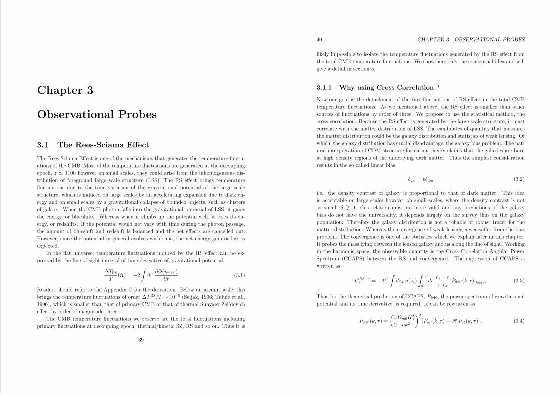
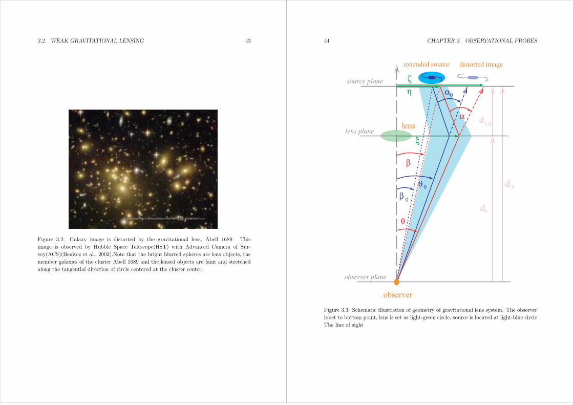
Figure 3.2: Galaxy image is distorted by the gravitational lens, Abell 1689. This
image is observed by Hubble Space Telescope(HST) with Advanced Camera of Sur-
vey(ACS)(Benitez et al., 2002).Note that the bright blurred spheres are lens objects, the
member galaxies of the cluster Abell 1689 and the lensed objects are faint and stretched
along the tangential direction of circle centered at the cluster center.
44 CHAPTER 3. OBSERVATIONAL PROBES
β
θ
extended source
observer
dL
β 0
θ 0
α0
α dLS
d S
lens
source plane
lens plane
observer plane
distorted image
ξ
η
ζ
Figure 3.3: Schematic illustration of geometry of gravitational lens system. The observer
is set to bottom point, lens is set as light-green circle, source is located at light-blue circle
The line of sight
3.2. WEAK GRAVITATIONAL LENSING 45
lens equation
First we consider the light deflection by single point mass M with the separation in the
lens plane being ξ = |ξ|. From the theory of general relativity, the deflection angle is
α(ξ) = 4GMξ
ξ2(3.7)
if the impact parameter ξ is enough larger than Schwarzschild radius, ξ Rs := 2GM .
This quantity is just twice of Newtonian theory’s one (e.g., Schneider et al., 1999).
We then extend the deflection by single mass to multiple point mass deflection. Imag-
ine that N point masses with their masses mi are putted in the lens plane with their loca-
tions ξi. Then the impact parameter vectors for each deflector masses are (ξ−ξi)/|ξ−ξi|2.In fact the mass distribution could be extended along the direction of line of sight how-
ever the protruberance is enough small compared to the distances, dLS, dL. Thus we can
approximate the mass distribution is confined within the lens plane. The total deflection
angle is then represented as the sum of contribution from each masses,
α(ξ) = 4GN∑i
miξ − ξi|ξ − ξi|2
(3.8)
Then we can take the continuum limit of equation (3.8), replacing the sum by an
integral. This is conveniently done by defining dm = Σ(ξ)d2ξ where d2ξ is surface ele-
ment in the lens plane, and Σ(ξ) is surface mass density, which is a projection of mass
distribution integrated along the line of sight onto the lens plane. Thus our assumption
made above that the mass distribution is confined within the lens plane is relaxed. Note
that this treatment still requires the condition that the extent of mass distribution to the
line of sight direction is small. Then the deflection angle becomes
α(ξ) = 4G
∫R2
d2ξ′ Σ(ξ′)ξ − ξ′
|ξ − ξ′|2 (3.9)
This equation is valid if the following conditions are satisfied.
• The gravitational field under consideration is weak, hence the deflection angle mustbe small.
• The mass distribution of lens along the line of sight is small compared to the angulardiameter distances from observer to lens and lens to source.
• The mass distribution of lens must be nearly stationary, i.e. the velocity of matterin the lens must be significantly smaller than the speed of light.
46 CHAPTER 3. OBSERVATIONAL PROBES
For the astrophysical situations, all these conditions are well satisfied and for the weak
lens analysis one should not be care about the violation of equation (3.9) as is the case
e.g. for the deflection by black holes.
Now we can derive the lens equation which relates the deflection angle to the source
image position. As illustrated in figure 3.3, let η and ξ denote the true position vector
in the source plane and image position in the lens plane respectively. In addition, let
ζ denote the image position projected on the source plane. Then from the definition
of angular diameter distance, ζ = dSθ and ζ = η + αdLS are satisfied. Therefore two
quantities expressing the angular vector θ must be equal, θ = ξ/dL = ζ/dS. This relation
is rewritten as
η =dSdL
ξ − dLSα (3.10)
Again recalling the definition of angular diameter distance, η = dSβ and ξ = dLθ yields
the lens equation
β = θ − dLSdS
α(dLθ) := θ −α(θ) (3.11)
For the system with multiple images this equation has more than one solutions, θ for fixed
β as is the case for strong lensing while for the system with single image, the solution is
unique. This can be conveniently quantified by the dimensionless surface mass density,
κ(θ) :=Σ(dLθ)
Σcr(3.12)
where the critical surface mass density is Σcr = dS/(4πGdLdLS). If κ ≥ 1 or equivalently
Σ ≥ Σcr somewhere in the lens plane, the system has multiple images. This is a sufficient
condition for producing multiple images but not necessary one. The scaled deflection
angle is then rewritten in terms of κ as
α(θ) =1
π
∫R2
d2θ′ κ(θ′)θ − θ′
|θ − θ′|2 (3.13)
As an analogical inference of Poisson equation in 3 dimensional space, we can consider
the 2 dimensional Poisson equation, ∆2Dψ(θ) = 2κ(θ), where ∆2D is 2 dimensional
Laplacian. Integral this Poisson equation over the lens plane, R2 yields
ψ(θ) =1
π
∫R2
d2θ′ κ(θ′) ln |θ − θ′| (3.14)
Equations (3.13), (3.14) imply that the deflection angle must satisfy α = ∇2Dψ.
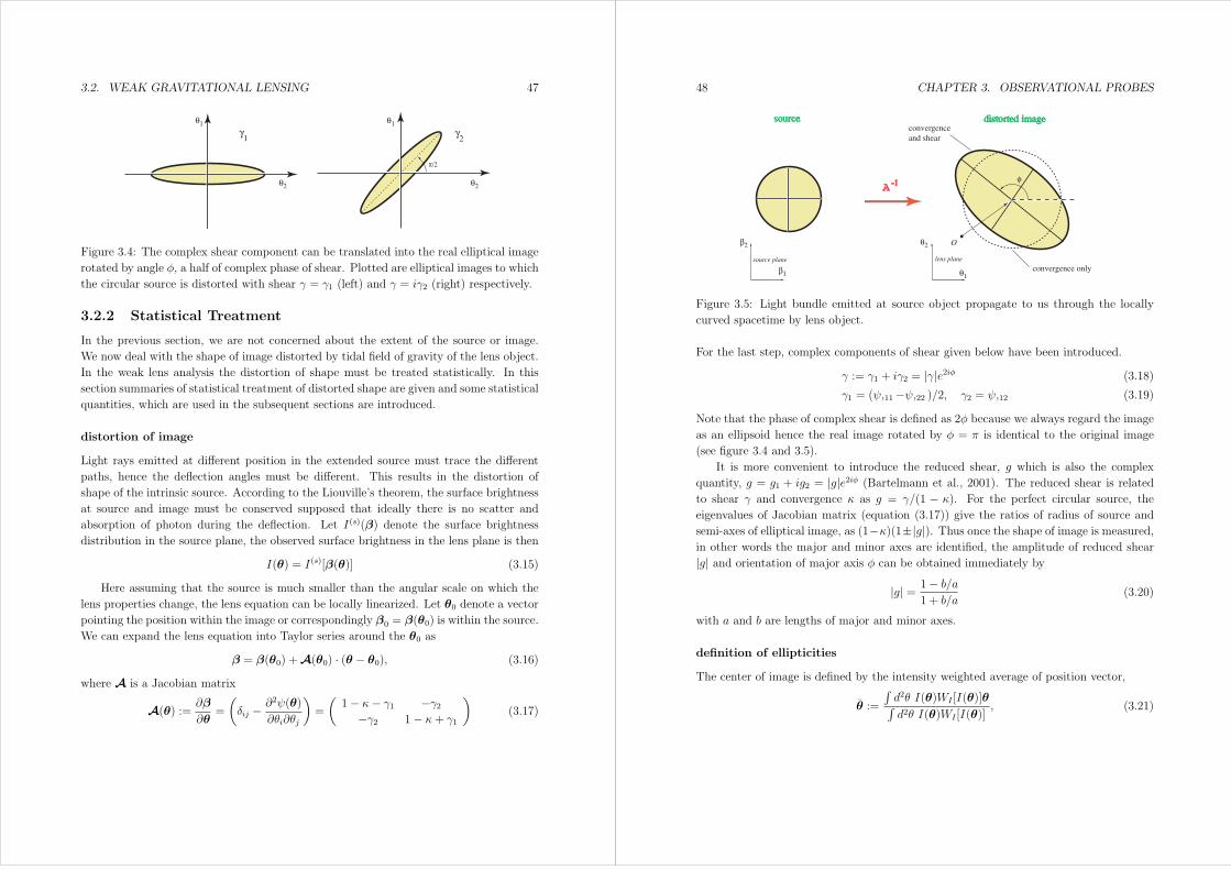
3.2. WEAK GRAVITATIONAL LENSING 47
γ1
γ2
θ1 θ1
θ2 θ2
π/2
Figure 3.4: The complex shear component can be translated into the real elliptical image
rotated by angle φ, a half of complex phase of shear. Plotted are elliptical images to which
the circular source is distorted with shear γ = γ1 (left) and γ = iγ2 (right) respectively.
3.2.2 Statistical Treatment
In the previous section, we are not concerned about the extent of the source or image.
We now deal with the shape of image distorted by tidal field of gravity of the lens object.
In the weak lens analysis the distortion of shape must be treated statistically. In this
section summaries of statistical treatment of distorted shape are given and some statistical
quantities, which are used in the subsequent sections are introduced.
distortion of image
Light rays emitted at different position in the extended source must trace the different
paths, hence the deflection angles must be different. This results in the distortion of
shape of the intrinsic source. According to the Liouville’s theorem, the surface brightness
at source and image must be conserved supposed that ideally there is no scatter and
absorption of photon during the deflection. Let I(s)(β) denote the surface brightness
distribution in the source plane, the observed surface brightness in the lens plane is then
I(θ) = I(s)[β(θ)] (3.15)
Here assuming that the source is much smaller than the angular scale on which the
lens properties change, the lens equation can be locally linearized. Let θ0 denote a vector
pointing the position within the image or correspondingly β0 = β(θ0) is within the source.
We can expand the lens equation into Taylor series around the θ0 as
β = β(θ0) +A(θ0) · (θ − θ0), (3.16)
where A is a Jacobian matrix
A(θ) := ∂β
∂θ=
(δij − ∂2ψ(θ)
∂θi∂θj
)=
(1− κ− γ1 −γ2−γ2 1− κ+ γ1
)(3.17)
48 CHAPTER 3. OBSERVATIONAL PROBES
source distorted image
convergence only
convergence
and shear
β2
β1 θ1
θ2 O
φA
-1
source plane lens plane
Figure 3.5: Light bundle emitted at source object propagate to us through the locally
curved spacetime by lens object.
For the last step, complex components of shear given below have been introduced.
γ := γ1 + iγ2 = |γ|e2iφ (3.18)
γ1 = (ψ,11−ψ,22 )/2, γ2 = ψ,12 (3.19)
Note that the phase of complex shear is defined as 2φ because we always regard the image
as an ellipsoid hence the real image rotated by φ = π is identical to the original image
(see figure 3.4 and 3.5).
It is more convenient to introduce the reduced shear, g which is also the complex
quantity, g = g1 + ig2 = |g|e2iφ (Bartelmann et al., 2001). The reduced shear is relatedto shear γ and convergence κ as g = γ/(1 − κ). For the perfect circular source, the
eigenvalues of Jacobian matrix (equation (3.17)) give the ratios of radius of source and
semi-axes of elliptical image, as (1−κ)(1±|g|). Thus once the shape of image is measured,in other words the major and minor axes are identified, the amplitude of reduced shear
|g| and orientation of major axis φ can be obtained immediately by
|g| = 1− b/a
1 + b/a(3.20)
with a and b are lengths of major and minor axes.
definition of ellipticities
The center of image is defined by the intensity weighted average of position vector,
θ :=
∫d2θ I(θ)WI [I(θ)]θ∫d2θ I(θ)WI [I(θ)]
, (3.21)
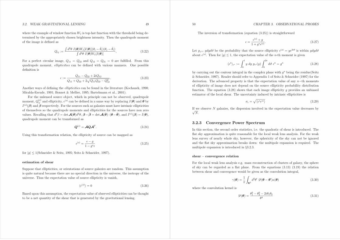
3.2. WEAK GRAVITATIONAL LENSING 49
where the example of window functionWI is top-hat function with the threshold being de-
termined by the appropriately chosen brightness intensity. Then the quadrupole moment
of the image is defined as
Qij :=
∫d2θ I(θ)WI [I(θ)](θi − θi)(θj − θi)∫
d2θ I(θ)WI [I(θ)], (3.22)
For a perfect circular image, Q11 = Q22 and Q12 = Q21 = 0 are fulfilled. From this
quadrupole moment, ellipticities can be defined with various manners. One possible
definition is
ε :=Q11 −Q22 + 2iQ12
Q11 +Q22 + 2√Q11Q22 −Q2
12
. (3.23)
Another ways of defining the ellipticities can be found in the literature (Kochanek, 1990;
Miralda-Escude, 1991; Bonnet & Mellier, 1995; Bartelmann et al., 2001).
For the unlensed source object, which in principle can not be observed, quadrupole
moment, Q(s)ij and ellipticity, ε(s) can be defined in a same way by replacing I(θ) and θ by
I(s)(β) and β respectively. For the sources such as galaxies must have intrinsic ellipticities
of themselves so the quadrupole moments and ellipticities for the sources have non zero
values. Recalling that d2β = detA(θ)d2θ, β− β = detA(θ) · (θ− θ), and I(s)(β) = I(θ),
quadrupole moment can be transformed as
Q(s) = AQAT . (3.24)
Using this transformation relation, the ellipticity of source can be mapped as
ε(s) =ε− g
1− g∗ε(3.25)
for |g| ≤ 1(Schneider & Seitz, 1995; Seitz & Schneider, 1997).
estimation of shear
Suppose that ellipticities, or orientations of source galaxies are random. This assumption
is quite natural because there are no special direction in the universe, the isotropy of the
universe. Thus the expectation value of source ellipticity is vanish,
〈ε(s)〉 = 0 (3.26)
Based upon this assumption, the expectation value of observed ellipticities can be thought
to be a net quantity of the shear that is generated by the gravitational lensing.
50 CHAPTER 3. OBSERVATIONAL PROBES
The inversion of transformation (equation (3.25)) is straightforward
ε =ε(s) + g
1 + g∗ε(s). (3.27)
Let pε(s) ydydϑ be the probability that the source ellipticity ε(s) = ye2iϑ is within ydydϑ
about ε(s). Then for |g| ≤ 1, the expectation value of the n-th moment is given
〈εn〉εs :=∫ 1
0
y dy pεs(y)
∫ 2π
0
dϑ εn = gn (3.28)
by carrying out the contour integral in the complex plane with gn being the residue(Seitz
& Schneider, 1997). Reader should refer to Appendix 1 of Seitz & Schneider (1997) for the
derivation. The advanced property is that the expectation value of any n−th momentsof ellipticity of image does not depend on the source ellipticity probability distribution
function. The equation (3.28) shows that each image ellipticity g provides an unbiased
estimator of the local shear. The uncertainty induced by intrinsic ellipticities is
σε =√〈εsεs∗〉 (3.29)
If we observe N galaxies, the dispersion involved in the expectation value decreases by√N .
3.2.3 Convergence Power Spectrum
In this section, the second order statistics, i.e. the quadratic of shear is introduced. The
flat sky approximation is quite reasonable for the local weak lens analysis. For the weak
lens survey of nearly whole sky, however, the sphericity of the sky can not be ignored
and the flat sky approximation breaks down: the multipole expansion is required. The
multipole expansion is introduced in §3.2.3.
shear – convergence relation
For the local weak lens analysis e.g. mass reconstruction of clusters of galaxy, the sphere
of sky can be regarded as a flat plane. From the equations (3.13) (3.19) the relation
between shear and convergence would be given as the convolution integral,
γ(θ) =1
π
∫R2
d2θ′ D(θ − θ′)κ(θ) (3.30)
where the convolution kernel is
D(θ) =θ21 − θ22 − 2iθ1θ2
θ4(3.31)

3.2. WEAK GRAVITATIONAL LENSING 51
(see e.g. Bartelmann et al., 2001) Thus in the Fourier space, this relation is simply ex-
pressed in the multiplication form. Based on the flat sky assumption (see the next section
for the spherical sky treatment), the convergence and shear which are defined on the 2
dimensional plane, is Fourier transformed as
κ() =
∫d2θ κ(θ)ei·θ, γ() =
∫d2θ γ(θ)ei·θ. (3.32)
Thus using the equation (3.30), the relation between complex shear and convergence can
be represented as
γ() =
(21 − 22 + 2i12
2
)κ() = e2iβκ() (3.33)
The coefficient of κ is Fourier counterpart of convolution kernel. Since its amplitude is
unity, convergence and shear is same amplitude and difference between them is only the
complex phase. Recalling the fact that the power spectrum discards the information of
phase, the power spectrum of convergence is identical to that of shear,
〈γ()γ∗(′)〉 = 〈κ()κ∗(′)〉 = (2π)2δD(− ′)P κ() (3.34)
As in the three dimensional power spectrum of matter, the power spectrum of convergence
depends only on the amplitude of wave vector , not on the angle β due to the isotropy
of the universe.
angular correlation
While in the previous, the convergence is a function of 2 dimensional plane, it must
be defined on a sphere of sky. Thus the convergence or shear should be expanded in a
spherical harmonic series. Henceforth the κ and γ are the function of polar and azimuthal
angles of the spherical coordinate.
κ(n) =∑,m
aκmYm(n) (3.35)
Following Jain & Seljak (1997), explicit form of angular power spectrum is derived (see
also Kaiser, 1998; Seljak, 1996, for another derivation). Recall that for the weak lens,
the deflection angle is small and the Jacobian matrix can be expressed with the Born
approximation. This yields that the deflection potential ψ is related to the Newtonian
potential as
ψ(n, r) = 2
∫ r
0
dr′r − r′
rr′Φ(r′n, r′) (3.36)
52 CHAPTER 3. OBSERVATIONAL PROBES
Here we introduce the argument r of ψ to stress the radial position of the source. This
expression is obtained by the first order perturbation from the non deflected trajectory
in the Born successive approximation. Higher order corrections are made by (Schneider
et al., 1998). Thus the convergence are related to the Newtonian potential as
κ(n, r) =
∫ r
0
dr′r − r′
rr′∇2Φ(rn, r′). (3.37)
Note that although originally κ is defined as the 2D Laplacian of ψ, it can be replaced
by the 3D Laplacian by just adding Φ,33 with 3 denoting the radial coordinate because
the radial curvature of the Newtonian potential does nothing with light deflection after
integrating along the line of sight. Substituting the expression of inverse Fourier transform
of Φ and using the Rayleigh expansion of plane wave (the basis of Fourier expansion), one
yields the angular power spectrum of the convergence,
Cκ (r1, r2) = 4π
∫dk
k
∫ r1
0
dr′1
∫ r2
0
dr′2 ∆2Φ(k, r
′1, r
′2)g(r
′1)g(r
′2)j(kr
′1)j(kr
′2), (3.38)
where the ∆2Φ is dimensionless power spectrum of gravitational potential, g(r) is the kernel
appeared in equation (3.37) and j is spherical Bessel function of order . This is a angular
power spectrum of sources lied at r1 and r2. For practical, the source must have some
sort of distribution pr(r). The angular power spectrum including source distribution is
then number density weighted projection.
Cκ =
∫dr1
∫dr2 pr(r1)pr(r2)C
κ (r1, r2) (3.39)
with the normalization being∫dr pr(r) =
∫dz n(z) = 1

Chapter 4
Non-linear Treatment
In the inflationary scenario, the initial fluctuations of matter, δ are generated such that
the explosive expansion of inflation elongates the quantum fluctuation and turns it to
classical density fluctuation (Kolb & Turner, 1990; Dvali et al., 2004). Since the amplitude
of initial fluctuation is very small, δ 1, one can treat the evolution of δ using the
linear perturbation theory. Here, the term linear stands for the first order deviation from
isotropic and homogeneous background density field.
As time goes on, the gravitational instability makes δ ∼ 1 and even δ 1. The
typical value of δ in the virialized cluster, is of order δvir 180 (Eke et al., 1996). For
such a case, the linear perturbation theory breaks down and some theories describing non-
linearity are required. The one approach involves higher order terms in the perturbation
theory (§4.1). Another approach is to consult a fitting formula to the large set of N -bodysimulations developed by Peacock & Dodds (1996); Smith et al. (2003) (§4.2). The otheris so-called halo approach (§4.3). Figure 4.1 shows non-linear evolution of matter powerspectrum with time. Plotted lines are calculated using the Smith et al.’s fitting formula
(solid line). The dashed lines are result of linear perturbation theory, and symbols show
the N -body simulations by Gadget-2 (Springel, 2005). It can be seen that the linear
theory can no more trace the true amplitude of matter clustering on small scales but the
fitting formula of Smith et al. well describes the non-linearity of matter power spectrum.
We refer to the term, non linearity as the deviation of any quantities from those of linear
theory predictions.
In this chapter, we develop the calculus of non-linear evolution of cross correlation
power spectrum between gravitational potential and its time derivative by applying a
couple of existing non-linear theories, partially including the review of existing theories;
the third order perturbation theory (3PT), fitting formula for the dark matter N -body
simulation, and the halo model. As we described at section 3.1.1, all we need to estimate
is the cross power spectrum of density and its time derivative, Pδδ′(k, z) involving the
53
54 CHAPTER 4. NON-LINEAR TREATMENT
k [h/Mpc]
∆2(k
)
z = 0z = 0.5
z = 2
z = 5
z = 10
Smith et al.2003
linear theory
N-body
Figure 4.1: Non-linear evolution of matter power spectrum.
non-linear treatment. We found that the results from N -body simulations show very
good agreement with the analytical predictions. We will discuss about the non linear
properties of the ΦΦ′ in the last section of this chapter.
4.1 Third Order Perturbation Theory
As a natural extension of linear perturbation theory, one might be tempted to use higher-
order perturbation theory to describe the non-linearity of evolution of matter. The evo-
lution of matter in an Einstein de-Sitter(EdS) background is solved analytically using
the third order perturbation theory (Suto & Sasaki, 1991; Makino et al., 1992; Jain &
Bertschinger, 1994). In a perturbative approach, one should keep a general assumption in
mind that the matter density can be treated as a fluid. Thus we can track the evolution
of matter by solving the continuity equation and Euler equation together with Poisson
equation in an expanding background spacetime. Therefore one should solve δ with θ, a
divergence of velocity in simultaneous equations order by order.
The density fluctuation and divergence of velocity is expanded in a series as,
δ(k, τ) =∞∑n=1
δn(k, τ), θ(k, τ) =∞∑n=1
θn(k, τ). (4.1)
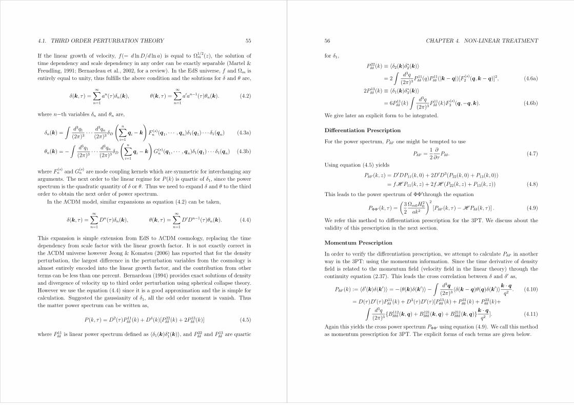
4.1. THIRD ORDER PERTURBATION THEORY 55
If the linear growth of velocity, f(= d lnD/d ln a) is equal to Ω1/2m (z), the solution of
time dependency and scale dependency in any order can be exactly separable (Martel &
Freudling, 1991; Bernardeau et al., 2002, for a review). In the EdS universe, f and Ωm is
entirely equal to unity, thus fulfills the above condition and the solutions for δ and θ are,
δ(k, τ) =∞∑n=1
an(τ)δn(k), θ(k, τ) =∞∑n=1
a′an−1(τ)θn(k). (4.2)
where n−th variables δn and θn are,
δn(k) =
∫d3q1(2π)3
· · · d3qn
(2π)3δD
(n∑i=1
qi − k
)F (s)n (q1, · · · , qn)δ1(q1) · · · δ1(qn) (4.3a)
θn(k) = −∫
d3q1(2π)3
· · · d3qn
(2π)3δD
(n∑i=1
qi − k
)G(s)n (q1, · · · , qn)δ1(q1) · · · δ1(qn) (4.3b)
where F(s)n and G
(s)n are mode coupling kernels which are symmetric for interchanging any
arguments. The next order to the linear regime for P (k) is quartic of δ1, since the power
spectrum is the quadratic quantity of δ or θ. Thus we need to expand δ and θ to the third
order to obtain the next order of power spectrum.
In the ΛCDM model, similar expansions as equation (4.2) can be taken,
δ(k, τ) =∞∑n=1
Dn(τ)δn(k), θ(k, τ) =∞∑n=1
D′Dn−1(τ)θn(k). (4.4)
This expansion is simple extension from EdS to ΛCDM cosmology, replacing the time
dependency from scale factor with the linear growth factor. It is not exactly correct in
the ΛCDM universe however Jeong & Komatsu (2006) has reported that for the density
perturbation, the largest difference in the perturbation variables from the cosmology is
almost entirely encoded into the linear growth factor, and the contribution from other
terms can be less than one percent. Bernardeau (1994) provides exact solutions of density
and divergence of velocity up to third order perturbation using spherical collapse theory.
However we use the equation (4.4) since it is a good approximation and the is simple for
calculation. Suggested the gaussianity of δ1, all the odd order moment is vanish. Thus
the matter power spectrum can be written as,
P (k, τ) = D2(τ)P 11δδ (k) +D4(k)[P 22
δδ (k) + 2P13δδ (k)] (4.5)
where P 11δδ is linear power spectrum defined as 〈δ1(k)δ∗1(k)〉, and P 22
δδ and P 13δδ are quartic
56 CHAPTER 4. NON-LINEAR TREATMENT
for δ1,
P 22δδ (k) ≡ 〈δ2(k)δ∗2(k)〉
= 2
∫d3q
(2π)3P 11δδ (q)P
11δδ (|k − q|)[F (s)
2 (q,k − q)]2, (4.6a)
2P 13δδ (k) ≡ 〈δ1(k)δ∗3(k)〉
= 6P 11δδ (k)
∫d3q
(2π)3P 11δδ (k)F
(s)3 (q,−q,k). (4.6b)
We give later an explicit form to be integrated.
Differentiation Prescription
For the power spectrum, Pδδ′ one might be tempted to use
Pδδ′ =1
2
∂
∂τPδδ. (4.7)
Using equation (4.5) yields
Pδδ′(k, z) = D′DP11(k, 0) + 2D′D3(P22(k, 0) + P13(k, 0))
= fH P11(k, z) + 2fH (P22(k, z) + P13(k, z)) (4.8)
This leads to the power spectrum of ΦΦ′through the equation
PΦΦ′(k, τ) =
(3
2
Ωm0H20
ak2
)2
[Pδδ′(k, τ)−H Pδδ(k, τ)] . (4.9)
We refer this method to differentiation prescription for the 3PT. We discuss about the
validity of this prescription in the next section.
Momentum Prescription
In order to verify the differentiation prescription, we attempt to calculate Pδδ′ in another
way in the 3PT: using the momentum information. Since the time derivative of density
field is related to the momentum field (velocity field in the linear theory) through the
continuity equation (2.37). This leads the cross correlation between δ and δ′ as,
Pδδ′(k) := 〈δ′(k)δ(k′)〉 = −〈θ(k)δ(k′)〉 −∫
d3q
(2π)3〈δ(k − q)θ(q)δ(k′)〉k · q
q2. (4.10)
= D(τ)D′(τ)P 11δδ (k) +D3(τ)D′(τ)[P 13
θδ (k) + P 31θδ (k) + P 22
θδ (k)+∫d3q
(2π)3B112
δθδ (k, q) +B121δθδ (k, q) +B211
δθδ (k, q)k · qq2
]. (4.11)
Again this yields the cross power spectrum PΦΦ′ using equation (4.9). We call this method
as momentum prescription for 3PT. The explicit forms of each terms are given below.
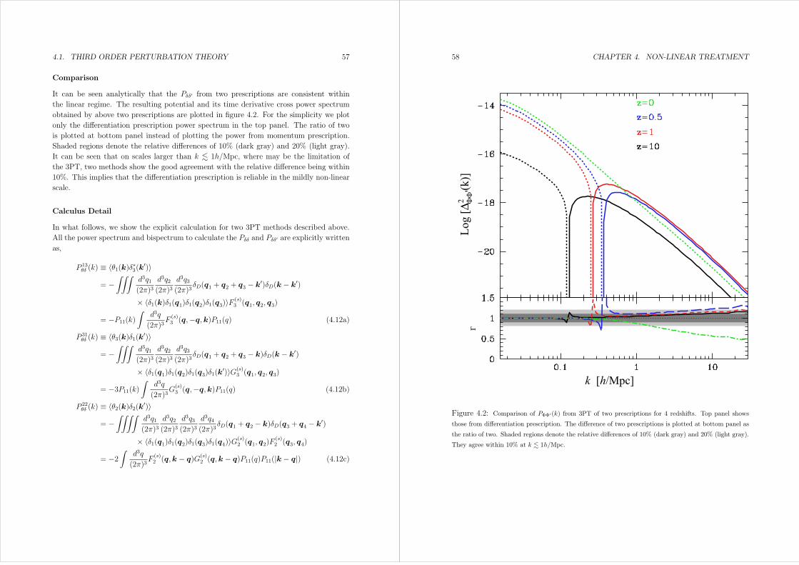
4.1. THIRD ORDER PERTURBATION THEORY 57
Comparison
It can be seen analytically that the Pδδ′ from two prescriptions are consistent within
the linear regime. The resulting potential and its time derivative cross power spectrum
obtained by above two prescriptions are plotted in figure 4.2. For the simplicity we plot
only the differentiation prescription power spectrum in the top panel. The ratio of two
is plotted at bottom panel instead of plotting the power from momentum prescription.
Shaded regions denote the relative differences of 10% (dark gray) and 20% (light gray).
It can be seen that on scales larger than k 1h/Mpc, where may be the limitation of
the 3PT, two methods show the good agreement with the relative difference being within
10%. This implies that the differentiation prescription is reliable in the mildly non-linear
scale.
Calculus Detail
In what follows, we show the explicit calculation for two 3PT methods described above.
All the power spectrum and bispectrum to calculate the Pδδ and Pδδ′ are explicitly written
as,
P 13θδ (k) ≡ 〈θ1(k)δ∗3(k′)〉
= −∫∫∫
d3q1(2π)3
d3q2(2π)3
d3q3(2π)3
δD(q1 + q2 + q3 − k′)δD(k − k′)
× 〈δ1(k)δ1(q1)δ1(q2)δ1(q3)〉F (s)3 (q1, q2, q3)
= −P11(k)∫
d3q
(2π)3F(s)3 (q,−q,k)P11(q) (4.12a)
P 31θδ (k) ≡ 〈θ3(k)δ1(k′)〉
= −∫∫∫
d3q1(2π)3
d3q2(2π)3
d3q3(2π)3
δD(q1 + q2 + q3 − k)δD(k − k′)
× 〈δ1(q1)δ1(q2)δ1(q3)δ1(k′)〉G(s)3 (q1, q2, q3)
= −3P11(k)∫
d3q
(2π)3G(s)3 (q,−q,k)P11(q) (4.12b)
P 22θδ (k) ≡ 〈θ2(k)δ2(k′)〉
= −∫∫∫∫
d3q1(2π)3
d3q2(2π)3
d3q3(2π)3
d3q4(2π)3
δD(q1 + q2 − k)δD(q3 + q4 − k′)
× 〈δ1(q1)δ1(q2)δ1(q3)δ1(q4)〉G(s)2 (q1, q2)F
(s)2 (q3, q4)
= −2∫
d3q
(2π)3F(s)2 (q,k − q)G
(s)2 (q,k − q)P11(q)P11(|k − q|) (4.12c)
58 CHAPTER 4. NON-LINEAR TREATMENT
k [h/Mpc]
Log [
∆2 (
k)]
ΦΦ
'
Figure 4.2: Comparison of PΦΦ′(k) from 3PT of two prescriptions for 4 redshifts. Top panel shows
those from differentiation prescription. The difference of two prescriptions is plotted at bottom panel as
the ratio of two. Shaded regions denote the relative differences of 10% (dark gray) and 20% (light gray).
They agree within 10% at k 1h/Mpc.
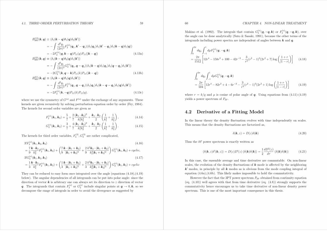
4.1. THIRD ORDER PERTURBATION THEORY 59
B112δθδ (k, q) ≡ 〈δ1(k − q)θ1(q)δ2(k
′)〉
= −∫
d3q1(2π)3
F(s)2 (q1,k
′ − q1)〈δ1(q1)δ1(k′ − q1)δ1(k − q)δ1(q)〉
= −2F (s)2 (q,k − q)P11(q)P11(|k − q|) (4.13a)
B121δθδ (k, q) ≡ 〈δ1(k − q)θ2(q)δ1(k
′)〉
= −∫
d3q1(2π)3
G(s)2 (q1, q − q1)〈δ1(k − q)δ1(q1)δ1(q − q1)δ1(k
′)〉
= −2G(s)2 (k, q − k)P11(k)P11(|k − q|) (4.13b)
B211δθδ (k, q) ≡ 〈δ2(k − q)θ1(q)δ1(k
′)〉
= −∫
d3q1(2π)3
F(s)2 (q1, q − q1)〈δ1(q1)δ1(k − q − q1)δ1(q)δ1(k
′)〉
= −2F (s)2 (k,−q)P11(k)P11(q). (4.13c)
where we use the symmetry of G(s) and F (s) under the exchange of any arguments. These
kernels are given recursively by solving perturbation equation order by order (Fry, 1984).
The kernels for second order variables are given as
F(s)2 (k1,k2) =
5
7+2
7
(k1 · k2)2k21k
22
+k1 · k22
(1
k21+1
k22
), (4.14)
G(s)2 (k1,k2) =
3
7+4
7
(k1 · k2)2k21k
22
+k1 · k22
(1
k21+1
k22
). (4.15)
The kernels for third order variables, F(3)3 , G
(3)3 are rather complicated,
3!F(s)3 (k1,k2,k3) (4.16)
=7
9
k · k3k23
F(s)2 (k1,k2) +
(7
9
k · (k1 + k2)
|k1 + k2|2 +2
9
k2k3 · (k1 + k2)
k23|k1 + k2|2)G(s)2 (k1,k2) + cyclic,
3!G(s)3 (k1,k2,k3) (4.17)
=1
3
k · k3k23
F(s)2 (k1,k2) +
(1
3
k · (k1 + k2)
|k1 + k2|2 +2
3
k2k3 · (k1 + k2)
k23|k1 + k2|2)G(s)2 (k1,k2) + cyclic
They can be reduced to easy form once integrated over the angle (equations (4.18),(4.19)
below). The angular dependencies of all integrands can be put into polar angle: since the
direction of vector k is arbitrary one can always set its direction to z direction of vector
q. The integrands that contain F(s)2 or G
(s)2 include singular points at q → 0,k, so we
decompose the range of integrals in order to avoid the divergence as suggested by
60 CHAPTER 4. NON-LINEAR TREATMENT
Makino et al. (1992). The integrals that contain G(s)3 (q,−q,k) or F
(s)3 (q,−q,k), over
the angle can be done analytically (Suto & Sasaki, 1991), because the other terms of the
integrands including power spectra are independent of angles between k and q.
∫ 2π
0
dqφ
∫ 1
−1dµF
(s)3 (q,−q,k)
=2π
1512
[12r4 − 158r2 + 100− 42r−2 − 3
r3(r2 − 1)3(2r2 + 7) log
(1 + r
|1− r|)]
(4.18)
∫ 2π
0
dqφ
∫ 1
−1dµG
(s)3 (q,−q,k)
=2π
504
[12r4 − 82r2 + 4− 6r−2 − 3
r3(r2 − 1)3(2r2 + 1) log
(1 + r
|1− r|)]
(4.19)
where r = k/q and µ is cosine of polar angle of q. Using equations from (4.11)-(4.19)
yields a power spectrum of Pδδ′ .
4.2 Derivative of a Fitting Model
In the linear theory the density fluctuation evolves with time independently on scales.
This means that the density fluctuations are factorized as,
δ(k, z) = D(z)δ(k) (4.20)
Thus the δδ′ power spectrum is exactly written as
〈δ(k, z)δ′(k, z)〉 = D(z)D′(z) 〈δ(k)δ(k)〉 = 1
2
dD2(z)
dτ〈δ(k)δ(k)〉 (4.21)
In this case, the ensemble average and time derivative are commutable. On non-linear
scales, the evolution of the density fluctuations of k mode is affected by the neighboring
k′ modes, in principle by all k modes as is obvious from the mode coupling integral of
equation (4.6a),(4.6b). This likely makes impossible to hold the commutativity.
However the fact that the 3PT power spectrum Pδδ′ obtained from continuity equation
(eq. (4.10)) well agrees with that from time derivative (eq. (4.8)) strongly supports the
commutativity hence encourages us to take time derivative of non-linear density power
spectrum. This is one of the most important consequence in this thesis.
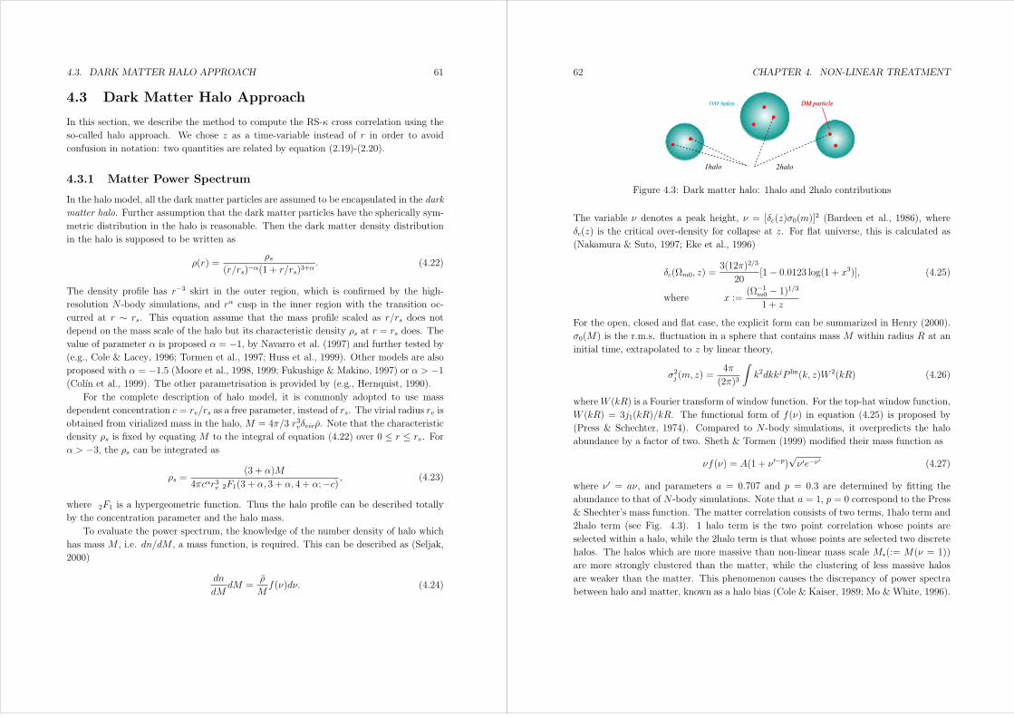
4.3. DARK MATTER HALO APPROACH 61
4.3 Dark Matter Halo Approach
In this section, we describe the method to compute the RS-κ cross correlation using the
so-called halo approach. We chose z as a time-variable instead of r in order to avoid
confusion in notation: two quantities are related by equation (2.19)-(2.20).
4.3.1 Matter Power Spectrum
In the halo model, all the dark matter particles are assumed to be encapsulated in the dark
matter halo. Further assumption that the dark matter particles have the spherically sym-
metric distribution in the halo is reasonable. Then the dark matter density distribution
in the halo is supposed to be written as
ρ(r) =ρs
(r/rs)−α(1 + r/rs)3+α. (4.22)
The density profile has r−3 skirt in the outer region, which is confirmed by the high-resolution N -body simulations, and rα cusp in the inner region with the transition oc-
curred at r ∼ rs. This equation assume that the mass profile scaled as r/rs does not
depend on the mass scale of the halo but its characteristic density ρs at r = rs does. The
value of parameter α is proposed α = −1, by Navarro et al. (1997) and further tested by(e.g., Cole & Lacey, 1996; Tormen et al., 1997; Huss et al., 1999). Other models are also
proposed with α = −1.5 (Moore et al., 1998, 1999; Fukushige & Makino, 1997) or α > −1(Colın et al., 1999). The other parametrisation is provided by (e.g., Hernquist, 1990).
For the complete description of halo model, it is commonly adopted to use mass
dependent concentration c = rv/rs as a free parameter, instead of rs. The virial radius rv is
obtained from virialized mass in the halo, M = 4π/3 r3vδvirρ. Note that the characteristic
density ρs is fixed by equating M to the integral of equation (4.22) over 0 ≤ r ≤ rv. For
α > −3, the ρs can be integrated as
ρs =(3 + α)M
4πcαr3v 2F1(3 + α, 3 + α, 4 + α;−c) , (4.23)
where 2F1 is a hypergeometric function. Thus the halo profile can be described totally
by the concentration parameter and the halo mass.
To evaluate the power spectrum, the knowledge of the number density of halo which
has mass M , i.e. dn/dM , a mass function, is required. This can be described as (Seljak,
2000)
dn
dMdM =
ρ
Mf(ν)dν. (4.24)
62 CHAPTER 4. NON-LINEAR TREATMENT
1halo 2halo
DM h DM particle
Figure 4.3: Dark matter halo: 1halo and 2halo contributions
The variable ν denotes a peak height, ν = [δc(z)σ0(m)]2 (Bardeen et al., 1986), where
δc(z) is the critical over-density for collapse at z. For flat universe, this is calculated as
(Nakamura & Suto, 1997; Eke et al., 1996)
δc(Ωm0, z) =3(12π)2/3
20[1− 0.0123 log(1 + x3)], (4.25)
where x :=(Ω−1
m0 − 1)1/31 + z
For the open, closed and flat case, the explicit form can be summarized in Henry (2000).
σ0(M) is the r.m.s. fluctuation in a sphere that contains mass M within radius R at an
initial time, extrapolated to z by linear theory,
σ2j (m, z) =4π
(2π)3
∫k2dkkjP lin(k, z)W 2(kR) (4.26)
whereW (kR) is a Fourier transform of window function. For the top-hat window function,
W (kR) = 3j1(kR)/kR. The functional form of f(ν) in equation (4.25) is proposed by
(Press & Schechter, 1974). Compared to N -body simulations, it overpredicts the halo
abundance by a factor of two. Sheth & Tormen (1999) modified their mass function as
νf(ν) = A(1 + ν ′−p)√ν ′e−ν′ (4.27)
where ν ′ = aν, and parameters a = 0.707 and p = 0.3 are determined by fitting the
abundance to that of N -body simulations. Note that a = 1, p = 0 correspond to the Press
& Shechter’s mass function. The matter correlation consists of two terms, 1halo term and
2halo term (see Fig. 4.3). 1 halo term is the two point correlation whose points are
selected within a halo, while the 2halo term is that whose points are selected two discrete
halos. The halos which are more massive than non-linear mass scale M∗(:= M(ν = 1))
are more strongly clustered than the matter, while the clustering of less massive halos
are weaker than the matter. This phenomenon causes the discrepancy of power spectra
between halo and matter, known as a halo bias (Cole & Kaiser, 1989; Mo & White, 1996).

4.3. DARK MATTER HALO APPROACH 63
The halo bias given by these authors is modified suitable for Sheth & Tormen’s mass
function as (Sheth & Tormen, 1999),
b(ν) = 1 +ν − 1δc
+2p
δc(1 + ν ′p)(4.28)
Since the halo is not point like but has finite extended profile. Thus the 2halo correlation
must be convolved with their halo profile of equation (4.22). Working in Fourier space
reduces the complications of the expression significantly (Scherrer & Bertschinger, 1991):
the convolution is replaced by multiplication. Thus the power spectrum of 2halo term is
the convolution of density fluctuations and Fourier transform of the halo profile with the
weight of mass function and halo bias integrated over all mass scales,
P 2hδδ (k; z) = P lin
δδ (k; z)
[∫dM n(M ; z)
M
ρu(k|M ; z)
]2, (4.29)
where u(k|M ; z) is Fourier transform of halo profile normalized by mass M ,
u(k|M ; z) =4π
M
∫r2dr ρ(r,M ; z)
sin(kr)
kr(4.30)
so that u(0|M ; z) = 1. This correlation become important on large scales and is identical
to linear theory prediction. Further correlation exists on small scales which comes from
the matter clustering within a same halo. This is given by the mass squared weighted
integral of mass function,
P 1hδδ (k; z) =
∫dM n(M ; z)
(M
ρ
)2
|u(k|M ; z)|2 (4.31)
The matter power spectrum is then given as a sum of two terms (Ma & Fry, 2000; Seljak,
2000),
Pδδ(k; z) = P 1hδδ (k; z) + P 2h
δδ (k; z) (4.32)
The three point function, and some third order statistics are found in (Ma & Fry, 2000)
using the halo model.
4.3.2 Momentum Power Spectrum
The momentum representation as in the 3PT is available also in the halo approach. The
momentum power spectrum is rather complex. The velocity of dark matter particle can
be decomposed into two terms : virial motion within a halo and bulk motion of the halo
itself (Sheth & Diaferio, 2001; Sheth et al., 2001),
v = vvir + vhalo. (4.33)
64 CHAPTER 4. NON-LINEAR TREATMENT
Figure 4.4: This figure is from (Seljak, 2000). Contribution to the P 1h(k) from different halo mass
intervals for the two models α = −1 (top) α = −1.5 (bottom). Short dashed lines from left to right are
1014h−1M < M , 1013h−1M < M < 1014h−1M, 1012h−1M < M < 1013h−1M and 1011h−1M <
M < 1012h−1M. Solid line is the total P (k), dotted the correlated term P 2h(k).
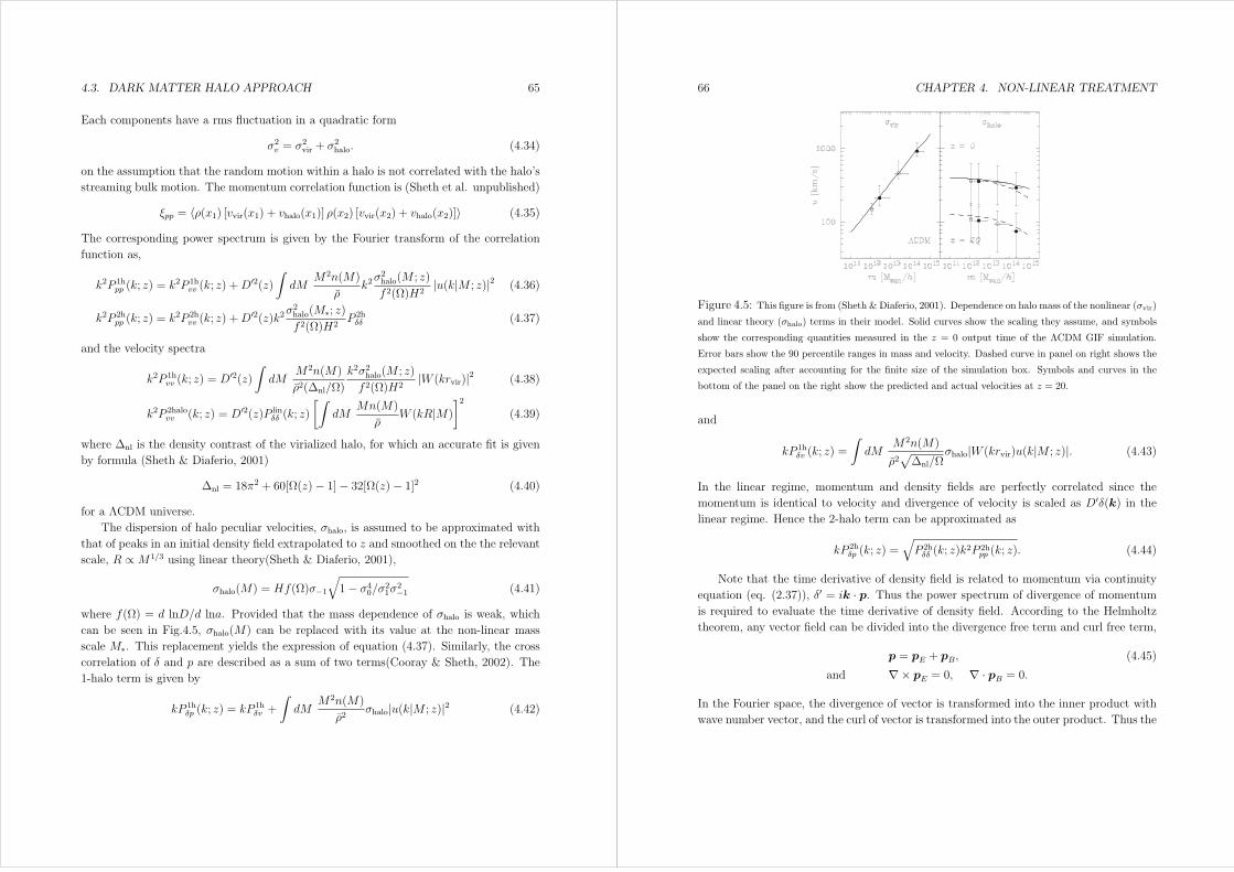
4.3. DARK MATTER HALO APPROACH 65
Each components have a rms fluctuation in a quadratic form
σ2v = σ2vir + σ2halo. (4.34)
on the assumption that the random motion within a halo is not correlated with the halo’s
streaming bulk motion. The momentum correlation function is (Sheth et al. unpublished)
ξpp = 〈ρ(x1) [vvir(x1) + vhalo(x1)] ρ(x2) [vvir(x2) + vhalo(x2)]〉 (4.35)
The corresponding power spectrum is given by the Fourier transform of the correlation
function as,
k2P 1hpp (k; z) = k2P 1h
vv (k; z) +D′2(z)∫
dMM2n(M)
ρk2
σ2halo(M ; z)
f2(Ω)H2|u(k|M ; z)|2 (4.36)
k2P 2hpp (k; z) = k2P 2h
vv (k; z) +D′2(z)k2σ2halo(M∗; z)f2(Ω)H2
P 2hδδ (4.37)
and the velocity spectra
k2P 1hvv (k; z) = D′2(z)
∫dM
M2n(M)
ρ2(∆nl/Ω)
k2σ2halo(M ; z)
f2(Ω)H2|W (krvir)|2 (4.38)
k2P 2halovv (k; z) = D′2(z)P lin
δδ (k; z)
[∫dM
Mn(M)
ρW (kR|M)
]2(4.39)
where ∆nl is the density contrast of the virialized halo, for which an accurate fit is given
by formula (Sheth & Diaferio, 2001)
∆nl = 18π2 + 60[Ω(z)− 1]− 32[Ω(z)− 1]2 (4.40)
for a ΛCDM universe.
The dispersion of halo peculiar velocities, σhalo, is assumed to be approximated with
that of peaks in an initial density field extrapolated to z and smoothed on the the relevant
scale, R ∝M1/3 using linear theory(Sheth & Diaferio, 2001),
σhalo(M) = Hf(Ω)σ−1√1− σ40/σ
21σ
2−1 (4.41)
where f(Ω) = d lnD/d lna. Provided that the mass dependence of σhalo is weak, which
can be seen in Fig.4.5, σhalo(M) can be replaced with its value at the non-linear mass
scale M∗. This replacement yields the expression of equation (4.37). Similarly, the crosscorrelation of δ and p are described as a sum of two terms(Cooray & Sheth, 2002). The
1-halo term is given by
kP 1hδp (k; z) = kP 1h
δv +
∫dM
M2n(M)
ρ2σhalo|u(k|M ; z)|2 (4.42)
66 CHAPTER 4. NON-LINEAR TREATMENT
Figure 4.5: This figure is from (Sheth & Diaferio, 2001). Dependence on halo mass of the nonlinear (σvir)
and linear theory (σhalo) terms in their model. Solid curves show the scaling they assume, and symbols
show the corresponding quantities measured in the z = 0 output time of the ΛCDM GIF simulation.
Error bars show the 90 percentile ranges in mass and velocity. Dashed curve in panel on right shows the
expected scaling after accounting for the finite size of the simulation box. Symbols and curves in the
bottom of the panel on the right show the predicted and actual velocities at z = 20.
and
kP 1hδv (k; z) =
∫dM
M2n(M)
ρ2√∆nl/Ω
σhalo|W (krvir)u(k|M ; z)|. (4.43)
In the linear regime, momentum and density fields are perfectly correlated since the
momentum is identical to velocity and divergence of velocity is scaled as D′δ(k) in thelinear regime. Hence the 2-halo term can be approximated as
kP 2hδp (k; z) =
√P 2hδδ (k; z)k
2P 2hpp (k; z). (4.44)
Note that the time derivative of density field is related to momentum via continuity
equation (eq. (2.37)), δ′ = ik · p. Thus the power spectrum of divergence of momentum
is required to evaluate the time derivative of density field. According to the Helmholtz
theorem, any vector field can be divided into the divergence free term and curl free term,
p = pE + pB, (4.45)
and ∇× pE = 0, ∇ · pB = 0.
In the Fourier space, the divergence of vector is transformed into the inner product with
wave number vector, and the curl of vector is transformed into the outer product. Thus the
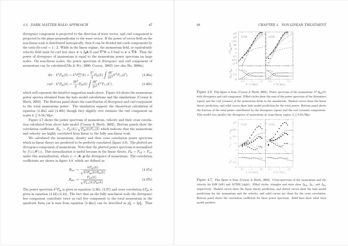
4.3. DARK MATTER HALO APPROACH 67
divergence component is projected to the direction of wave vector, and curl component is
projected to the plane perpendicular to the wave vector. If the power of vector field on the
non-linear scale is distributed isotropically, then it can be divided into each components by
the ratio div:curl = 1 : 2. While in the linear regime, the momentum field, or equivalently
velocity field must be curl free since v ∝ δkk/k and ∇2Φ ∝ δ lead to v ∝ ∇Φ. Thus thepower of divergence of momentum is equal to the momentum power spectrum on large
scales. On non-linear scales, the power spectrum of divergence and curl component of
momentum can be calculated(Ma & Fry, 2000; Cooray, 2002) (see also Hu, 2000a),
div : k2Ppp(k) = k2P linvv (k) +
k2
3Pδδ(k)
∫dk′
2π2k′2Pvv(k′), (4.46a)
curl : k2Ppp(k) =2k2
3Pδδ(k)
∫dk′
2π2k′2Pvv(k′), (4.46b)
which well represent the intuitive suggestion made above. Figure 4.6 shows the momentum
power spectra obtained from the halo model calculations and the simulations (Cooray &
Sheth, 2002). The Bottom panel shows the contribution of divergence and curl component
to the total momentum power. The simulation support the theoretical calculation of
equation (4.46a) and (4.46b) though they slightly over estimate the curl component on
scales k 0.5h/Mpc.
Figure 4.7 shows the power spectrum of momentum, velocity and their cross correla-
tion calculated from above halo model (Cooray & Sheth, 2002). Bottom panels show the
correlation coefficient, Rpv := Ppv(k)/√Ppp(k)Pvv(k) which indicate that the momentum
and velocity are highly correlated from linear to the fully non-linear scale.
We calculated the momentum, density and their cross correlation power spectrum
which in linear theory are predicted to be perfectly correlated (figure 4.9). The plotted are
divergence component of momentum. Note that the plotted power spectrum is normalized
by f(z)H (z). This normalization is useful because in the linear theory, Pδδ = Pψδ = Pψψunder this normalization, where ψ := ik ·p the divergence of momentum. The correlationcoefficients are shown in figure 4.8, which are defined as
Rtot :=kPpδ(k)√
k2Ppp(k)Pδδ(k), (4.47a)
Rdiv :=Pψδ(k)√
Pψψ(k)Pδδ(k)(4.47b)
The power spectrum k2Ppp is given in equation (4.36), (4.37) and cross correlation kPpδ is
given in equation (4.42)-(4.44). The fact that on the fully non-linear scale the divergence
free component contribute twice as curl free component to the total momentum in the
quadratic form (as is seen from equation (4.46a)) can be described as p2B = 2p2E. Thus
68 CHAPTER 4. NON-LINEAR TREATMENT
Figure 4.6: This figure is from (Cooray & Sheth, 2002). Power spectrum of the momentum: k2 ∆pp(k)
with divergence and curl component. Filled circles show the sum of the power spectrum of the divergence
(open) and the curl (crosses) of the momentum fields in the simulations. Dashed curves show the linear
theory prediction, and solid curves show halo model prediction for the total power. Bottom panel shows
the fraction of the total power contributed by the divergence (open) and the curl (crosses) components.
This model over predict the divergence of momentum at trans-linear region, k 0.5h/Mpc.
Figure 4.7: This figure is from (Cooray & Sheth, 2002). Cross-spectrum of the momentum and the
velocity for EdS (left) and ΛCDM (right). Filled circles, triangles and stars show ∆pp, ∆vv and ∆pv
respectively. Dashed curves show the linear theory prediction, and dotted curves show the halo model
predictions for the momentum and the velocity, and solid curves are those for the cross correlation.
Bottom panel shows the correlation coefficient for these power spectrum. Solid lines show what their
model predicts.

4.3. DARK MATTER HALO APPROACH 69
provided that pB ∼√2pE, then the divergence component of cross correlation, Pψδ(k)
can be approximated as
Pψδ(k) (2−√2)kfH P lin
δδ (k) + (√2− 1)kPpδ(k) (4.48)
This approximation is reasonable only at high redshift where the non-linearity is weak.
While for lower redshifts it significantly over-estimates the cross correlation between δ and
ψ. It can be seen in figure 4.8 that the divergence of momentum and density field is poorly
correlated at high-k, though the halo model predicts that the total momentum vs density
are totally correlated to the fully non-linear scale. The weak correlation between ψ and
δ at high-k is partially accounted for the fact that the divergence component which may
be correlated with density field is one third of total momentum. However the simulation
results pointed out the much weaker correlation than expected. The reason of this has
not been resolved and further investigations are required about the halo model.
70 CHAPTER 4. NON-LINEAR TREATMENT
z = 9.5z = 4.8z = 2.7z = 1.0z = 0.5z = 0.05
Figure 4.8: (top) The correlation coefficient between total momentum and density given by equation
(4.47a). The total momentum and density is almost perfectly correlated over the all scale. (bottom)
The correlation coefficient between ψ and density (equation (4.47b)). The solid lines are halo model
predictions and symbols are result from N -body simulations. The redshifts are from top to bottom,
z = 9.5, 4.8, 2.7, 1.0, 0.5, 0.05.
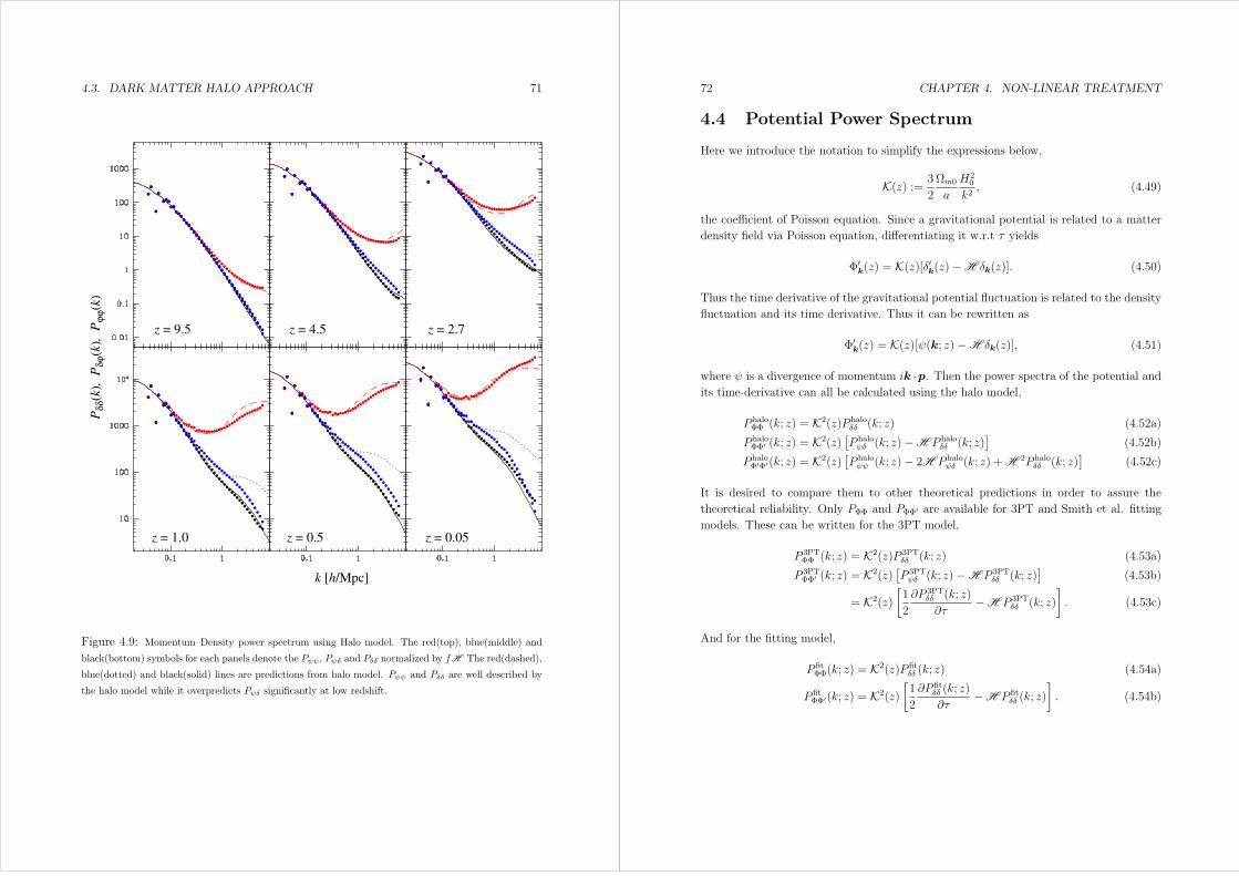
4.3. DARK MATTER HALO APPROACH 71
z = 9.5 z = 4.5 z = 2.7
z = 1.0 z = 0.5 z = 0.05
k [h/Mpc]
Pδδ(k
), P
δϕ(k
), P
ϕϕ(k
)
Figure 4.9: Momentum–Density power spectrum using Halo model. The red(top), blue(middle) and
black(bottom) symbols for each panels denote the Pψψ, Pψδ and Pδδ normalized by fH The red(dashed),
blue(dotted) and black(solid) lines are predictions from halo model. Pψψ and Pδδ are well described by
the halo model while it overpredicts Pψδ significantly at low redshift.
72 CHAPTER 4. NON-LINEAR TREATMENT
4.4 Potential Power Spectrum
Here we introduce the notation to simplify the expressions below,
K(z) := 3
2
Ωm0
a
H20
k2, (4.49)
the coefficient of Poisson equation. Since a gravitational potential is related to a matter
density field via Poisson equation, differentiating it w.r.t τ yields
Φ′k(z) = K(z)[δ′k(z)−H δk(z)]. (4.50)
Thus the time derivative of the gravitational potential fluctuation is related to the density
fluctuation and its time derivative. Thus it can be rewritten as
Φ′k(z) = K(z)[ψ(k; z)−H δk(z)], (4.51)
where ψ is a divergence of momentum ik ·p. Then the power spectra of the potential andits time-derivative can all be calculated using the halo model,
P haloΦΦ (k; z) = K2(z)P halo
δδ (k; z) (4.52a)
P haloΦΦ′ (k; z) = K2(z)
[P haloψδ (k; z)−H P halo
δδ (k; z)]
(4.52b)
P haloΦ′Φ′(k; z) = K2(z) [P halo
ψψ (k; z)− 2H P haloψδ (k; z) +H 2P halo
δδ (k; z)]
(4.52c)
It is desired to compare them to other theoretical predictions in order to assure the
theoretical reliability. Only PΦΦ and PΦΦ′ are available for 3PT and Smith et al. fitting
models. These can be written for the 3PT model,
P 3PTΦΦ (k; z) = K2(z)P 3PT
δδ (k; z) (4.53a)
P 3PTΦΦ′ (k; z) = K2(z)
[P 3PTψδ (k; z)−H P 3PT
δδ (k; z)]
(4.53b)
= K2(z)[1
2
∂P 3PTδδ (k; z)
∂τ−H P 3PT
δδ (k; z)
]. (4.53c)
And for the fitting model,
P fitΦΦ(k; z) = K2(z)P fit
δδ (k; z) (4.54a)
P fitΦΦ′(k; z) = K2(z)
[1
2
∂P fitδδ (k; z)
∂τ−H P fit
δδ (k; z)
]. (4.54b)
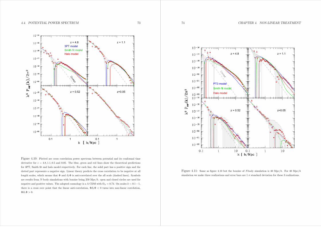
4.4. POTENTIAL POWER SPECTRUM 73
3PT model
Halo modelSmith fit model
z = 4.8 z = 1.1
0.1 1
z = 0.52
0.1 1
z=0.05
Figure 4.10: Plotted are cross correlation power spectrum between potential and its conformal time
derivative for z = 4.8, 1.1, 0.5 and 0.05. The blue, green and red lines show the theoretical predictions
for 3PT, Smith fit and halo model respectively. For each line, the solid part has a positive sign and the
dotted part represents a negative sign. Linear theory predicts the cross correlation to be negative at all
length scales, which means that Φ and ∂τΦ is anti-correlated over the all scale (dashed lines). Symbols
are results from N -body simulations with boxsize being 250 Mpc/h. open and closed circles are used for
negative and positive values. The adopted cosmology is a Λ CDM with ΩΛ = 0.74. On scales k ∼ 0.1−1,there is a cross over point that the linear anti-correlation, Φ∂τΦ < 0 turns into non-linear correlation,
Φ∂τΦ > 0.
74 CHAPTER 4. NON-LINEAR TREATMENT
Halo model
PT3 model
Smith fit model
z = 4.8 z = 1.1
z = 0.52 z=0.05
Figure 4.11: Same as figure 4.10 but the boxsize of Nbody simulation is 40 Mpc/h. For 40 Mpc/h
simulation we make three realizations and error bars are 1 σ standard deviation for these 3 realizations.
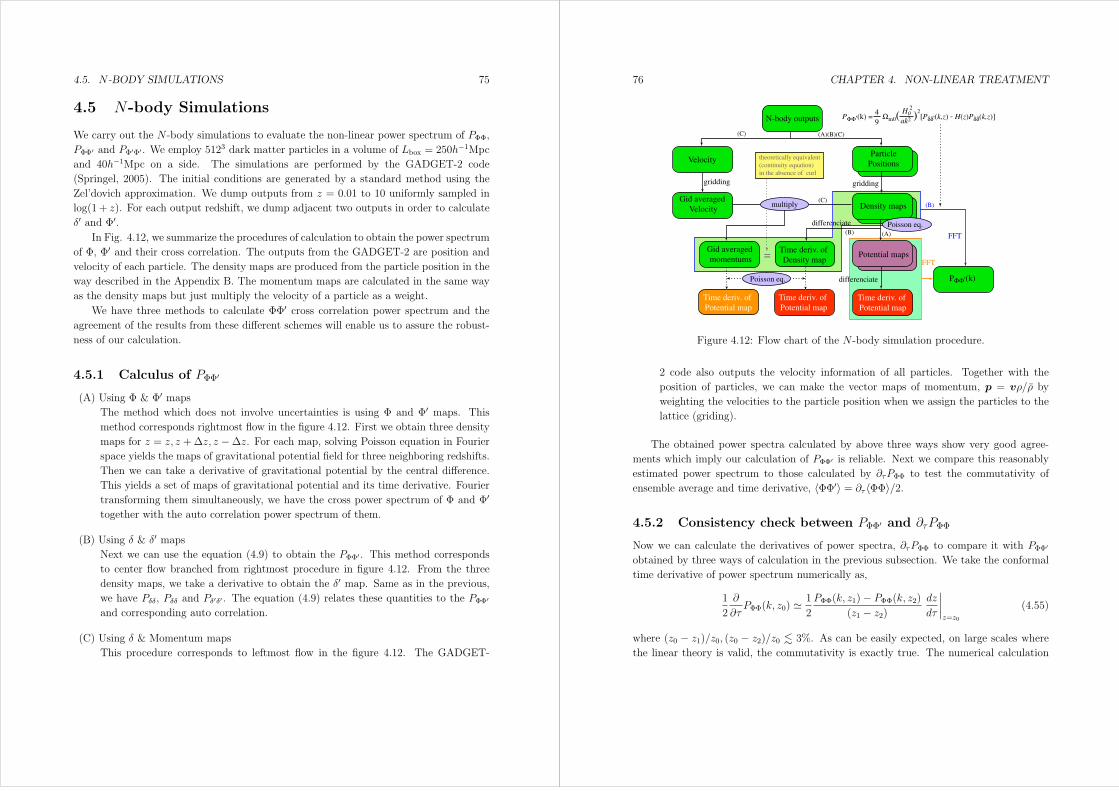
4.5. N -BODY SIMULATIONS 75
4.5 N-body Simulations
We carry out the N -body simulations to evaluate the non-linear power spectrum of PΦΦ,
PΦΦ′ and PΦ′Φ′ . We employ 5123 dark matter particles in a volume of Lbox = 250h−1Mpcand 40h−1Mpc on a side. The simulations are performed by the GADGET-2 code
(Springel, 2005). The initial conditions are generated by a standard method using the
Zel’dovich approximation. We dump outputs from z = 0.01 to 10 uniformly sampled in
log(1 + z). For each output redshift, we dump adjacent two outputs in order to calculate
δ′ and Φ′.In Fig. 4.12, we summarize the procedures of calculation to obtain the power spectrum
of Φ, Φ′ and their cross correlation. The outputs from the GADGET-2 are position and
velocity of each particle. The density maps are produced from the particle position in the
way described in the Appendix B. The momentum maps are calculated in the same way
as the density maps but just multiply the velocity of a particle as a weight.
We have three methods to calculate ΦΦ′ cross correlation power spectrum and the
agreement of the results from these different schemes will enable us to assure the robust-
ness of our calculation.
4.5.1 Calculus of PΦΦ′
(A) Using Φ & Φ′ mapsThe method which does not involve uncertainties is using Φ and Φ′ maps. Thismethod corresponds rightmost flow in the figure 4.12. First we obtain three density
maps for z = z, z +∆z, z −∆z. For each map, solving Poisson equation in Fourier
space yields the maps of gravitational potential field for three neighboring redshifts.
Then we can take a derivative of gravitational potential by the central difference.
This yields a set of maps of gravitational potential and its time derivative. Fourier
transforming them simultaneously, we have the cross power spectrum of Φ and Φ′
together with the auto correlation power spectrum of them.
(B) Using δ & δ′ mapsNext we can use the equation (4.9) to obtain the PΦΦ′ . This method corresponds
to center flow branched from rightmost procedure in figure 4.12. From the three
density maps, we take a derivative to obtain the δ′ map. Same as in the previous,we have Pδδ, Pδδ and Pδ′δ′ . The equation (4.9) relates these quantities to the PΦΦ′
and corresponding auto correlation.
(C) Using δ & Momentum maps
This procedure corresponds to leftmost flow in the figure 4.12. The GADGET-
76 CHAPTER 4. NON-LINEAR TREATMENT
N-body outputs
Velocity
Gid averaged
Velocity
Particle
Positions
Density maps
Time deriv. of
Density map
Gid averaged
momentumsPotential maps
Time deriv. of
Potential map
Time deriv. of
Potential map
Time deriv. of
Potential map
FFT
multiply
griddinggridding
theoretically equivalent
(continuity equation)
in the absence of curl
=
PΦΦ'(k)
PΦΦ'(k) = Ωm0( )2[Pδδ'(k,z) - H(z)Pδδ(k,z)]
4
9
H0
ak2
2
differenciatePoisson eq.
FFT
differenciate Poisson eq.
(A)(B)(C)
(C)
(A)(B)
(B)
(C)
Figure 4.12: Flow chart of the N -body simulation procedure.
2 code also outputs the velocity information of all particles. Together with the
position of particles, we can make the vector maps of momentum, p = vρ/ρ by
weighting the velocities to the particle position when we assign the particles to the
lattice (griding).
The obtained power spectra calculated by above three ways show very good agree-
ments which imply our calculation of PΦΦ′ is reliable. Next we compare this reasonably
estimated power spectrum to those calculated by ∂τPΦΦ to test the commutativity of
ensemble average and time derivative, 〈ΦΦ′〉 = ∂τ 〈ΦΦ〉/2.
4.5.2 Consistency check between PΦΦ′ and ∂τPΦΦ
Now we can calculate the derivatives of power spectra, ∂τPΦΦ to compare it with PΦΦ′
obtained by three ways of calculation in the previous subsection. We take the conformal
time derivative of power spectrum numerically as,
1
2
∂
∂τPΦΦ(k, z0) 1
2
PΦΦ(k, z1)− PΦΦ(k, z2)
(z1 − z2)
dz
dτ
∣∣∣∣z=z0
(4.55)
where (z0 − z1)/z0, (z0 − z2)/z0 3%. As can be easily expected, on large scales where
the linear theory is valid, the commutativity is exactly true. The numerical calculation

4.5. N -BODY SIMULATIONS 77
0.19.3 2.4
Figure 4.13: (Top) Power spectrum of Φ and ∂τΦ calculated from 250h−1Mpc N -body simulations
at various epochs between z ∼ 10 to 0.01, which are logarithmically uniformly sampled; they are, from
black to blue, z = 9.3, 7.2, 5.6, 4.3, 3.2, 2.4, 1.7, 1.1, 0.71, 0.37 and 0.096. Lines with points denote
positive, the non-linear effect, and those without points denote negative, the linear effect. Plotted are
dimensionless power spectrum, k3P (k)/2π. (Bottom) Fractional differences between PΦΦ′ and ∂τPΦΦ/2.
This quantifies the commutativity of ensemble average and time derivative of gravitational potential
directly. The commutativity is guaranteed within 1% error on scales k 0.2h/Mpc, and within 10% on
scales k 1h/Mpc. Scales smaller than k 3h/Mpc, the differences are significant.
78 CHAPTER 4. NON-LINEAR TREATMENT
0.19.3 2.4
Figure 4.14: Same as figure 4.13, but use 40h−1 Mpc boxsize simulations.
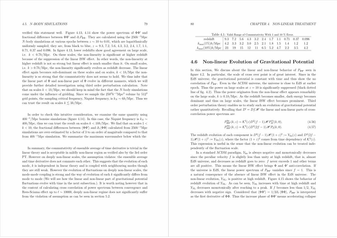
4.5. N -BODY SIMULATIONS 79
verified this statement well. Figure 4.13, 4.14 show the power spectrum of ΦΦ′ andfractional difference between ΦΦ′ and ∂τPΦΦ. They are calculated using the 250h
−1MpcN -body simulations at various epochs between z ∼ 10 to 0.01, which are logarithmically
uniformly sampled; they are, from black to blue, z = 9.3, 7.2, 5.6, 4.3, 3.2, 2.4, 1.7, 1.1,
0.71, 0.37 and 0.096. In figure 4.13, lower redshifts show good agreement on large scale,
i.e. k < 0.7h/Mpc. On these scales, the non-linearity is significant at higher redshift
because of the suppression of the linear ISW effect. In other words, the non-linearity at
higher redshift is not so strong but linear effect is much smaller than it. On small scales,
i.e. k > 0.7h/Mpc, the non-linearity significantly evolves as redshift decrease. The linear
effect again becomes sub-dominant on these scales and on scales, k < 1h/Mpc the non-
linearity is so strong that the commutativity does not seems to hold. We thus infer that
the linear part of Φ and non-linear part of Φ evolve in different manners, which we will
provide further detailed investigation using third order perturbation calculation. Note
that on scales k < 1h/Mpc, we should keep in mind the fact that the N -body simulations
come under the influence of gridding. Since we sample the 2503h−1Mpc3 volume by 5123
grid points, the sampling critical frequency, Niquist frequency, is kN ∼ 6h/Mpc. Thus we
can trust the result on scales k 3h/Mpc.
In order to check this intuitive consideration, we examine the same quantity using
40h−1/Mpc boxsize simulations (figure 4.14). In this case, the Niquist frequency is kN ∼40h/Mpc, thus we can trust the result on scales k < 10h/Mpc. We find that on scales 1 <
k < 10, the fractional differences between 〈ΦΦ′〉 and ∂τ 〈ΦΦ〉 calculated from 250h−1Mpcsimulations are over-estimated by a factor of 3 to an order of magnitude compared to that
from 40h−1Mpc simulation. We summarize the maximum wavenumber below which the
In summary, the commutativity of ensemble average of time derivative is trivial in the
linear theory and is acceptable in mildly non-linear region as verified also by the 3rd order
PT. However on deeply non-linear scales, the assumption violates: the ensemble average
and time derivative does not commute each other. This suggests that the evolution of each
mode, k is independent in linear theory and is coupled with neighbouring modes though
they are still weak. However the evolution of fluctuations on deeply non-linear scales, the
mode-mode coupling is strong and the way of evolution of each k significantly differs from
mode to mode (We will see how the linear and non-linear part of gravitational potential
fluctuations evolve with time in the next subsection.). It is worth noting however that in
the context of calculating cross correlation of power spectrum between convergence and
Rees-Sciama effect up to ∼ 10000, deeply non-linear regime does not significantly suffer
from the violation of assumption as can be seen in section 5.2.
80 CHAPTER 4. NON-LINEAR TREATMENT
Table 4.1: Valid Range of Commutativity With 1 and 10 % Error.
redshift 9.3 7.2 5.6 4.3 3.2 2.4 1.7 1.1 0.71 0.37 0.096
kmax(1%)h/Mpc 4.2 3.3 3.2 3.0 2.5 2.1 1.8 1.5 1.4 1.2 1.2
kmax(10%)h/Mpc 23 19 15 12 11 6.5 5.2 4.7 2.2 3.5 4.2
4.6 Non-linear Evolution of Gravitational Potential
In this section, We discuss about the linear and non-linear behavior of PΦΦ′ seen in
figure 4.2. In particular, the scale of cross over point is of great interest. Since in the
EdS universe, the gravitational potential is constant with time and thus show the no
correlation of PΦΦ′ . Even in the ΛCDM universe, the universe is close to EdS at earlier
epoch. Thus the power on large scales at z = 10 is significantly suppressed (black dotted
line of fig. 4.2). Thus the power originates from the non-linear effect appears remarkably
on the large scale, k 0.1h/Mpc. As the redshift becomes smaller, dark energy becomes
dominant and thus on large scales, the linear ISW effect becomes prominent. Third
order perturbation theory enables us to study such an evolution of gravitational potential
rather quantitatively. Recalling that D′ = DfH the linear and non-linear parts of cross-
correlation power spectrum are
P linΦΦ′(k, z) = K2(z)D2(f − 1)H P 11
δδ (k, 0), (4.56)
PNLΦΦ′(k, z) = K2(z)D4(2f − 1)H P2(k, 0). (4.57)
The redshift evolution of each component is D2(f − 1)H (1 + z)2 := Ylin(z) and D4(2f −1)H (1 + z)2 := YNL(z), where the factor (1 + z)2 comes from time dependency of K2(z).This expression is useful in the sense that the non-linear evolution can be treated inde-
pendently of the fluctuation scale.
In a standard ΛCDM paradigm, Ylin is always negative and monotonically decreases
since the peculiar velocity f is slightly less than unity at high redshift, that is, almost
EdS universe, and decreases as redshift goes to zero: f never exceeds 1 and other terms
are all positive. This means the linear ISW effect brings Φ and Φ′ anti-correlation. Ifthe universe is EdS, the linear power spectrum of PΦΦ′ vanishes since f = 1. This is
a natural consequence of the absence of linear ISW effect in the EdS universe. The
non-linear evolution, YNL, is positive at high redshift. Figure 4.15 shows the behavior of
redshift evolution of YNL. As can be seen, YNL increases with time at high redshift and
YNL decreases monotonically after reaching to a peak. If f becomes less than 1/2, YNLdecreases with negative sign. Considered that 〈ΦΦ′〉 = 1/2∂τ 〈ΦΦ〉, PΦΦ′ is interpreted
as the first derivative of ΦΦ. Thus the increase phase of ΦΦ′ means accelerating collapse
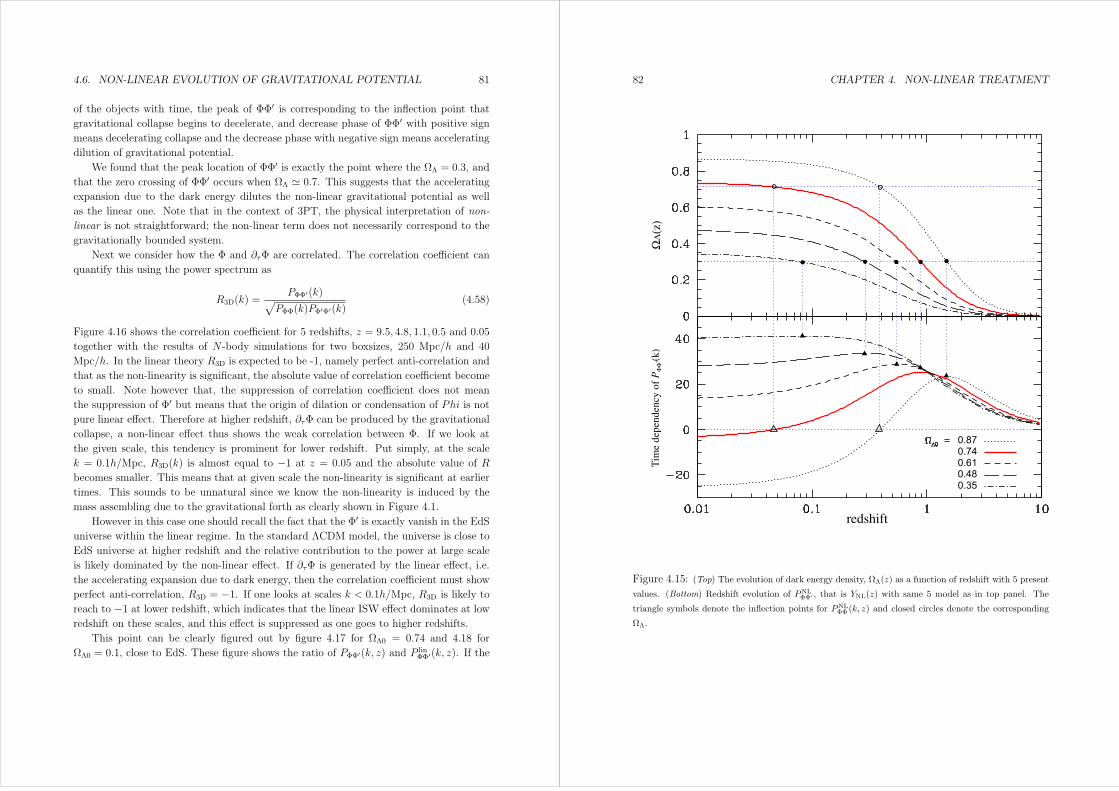
4.6. NON-LINEAR EVOLUTION OF GRAVITATIONAL POTENTIAL 81
of the objects with time, the peak of ΦΦ′ is corresponding to the inflection point thatgravitational collapse begins to decelerate, and decrease phase of ΦΦ′ with positive signmeans decelerating collapse and the decrease phase with negative sign means accelerating
dilution of gravitational potential.
We found that the peak location of ΦΦ′ is exactly the point where the ΩΛ = 0.3, and
that the zero crossing of ΦΦ′ occurs when ΩΛ 0.7. This suggests that the accelerating
expansion due to the dark energy dilutes the non-linear gravitational potential as well
as the linear one. Note that in the context of 3PT, the physical interpretation of non-
linear is not straightforward; the non-linear term does not necessarily correspond to the
gravitationally bounded system.
Next we consider how the Φ and ∂τΦ are correlated. The correlation coefficient can
quantify this using the power spectrum as
R3D(k) =PΦΦ′(k)√
PΦΦ(k)PΦ′Φ′(k)(4.58)
Figure 4.16 shows the correlation coefficient for 5 redshifts, z = 9.5, 4.8, 1.1, 0.5 and 0.05
together with the results of N -body simulations for two boxsizes, 250 Mpc/h and 40
Mpc/h. In the linear theory R3D is expected to be -1, namely perfect anti-correlation and
that as the non-linearity is significant, the absolute value of correlation coefficient become
to small. Note however that, the suppression of correlation coefficient does not mean
the suppression of Φ′ but means that the origin of dilation or condensation of Phi is notpure linear effect. Therefore at higher redshift, ∂τΦ can be produced by the gravitational
collapse, a non-linear effect thus shows the weak correlation between Φ. If we look at
the given scale, this tendency is prominent for lower redshift. Put simply, at the scale
k = 0.1h/Mpc, R3D(k) is almost equal to −1 at z = 0.05 and the absolute value of R
becomes smaller. This means that at given scale the non-linearity is significant at earlier
times. This sounds to be unnatural since we know the non-linearity is induced by the
mass assembling due to the gravitational forth as clearly shown in Figure 4.1.
However in this case one should recall the fact that the Φ′ is exactly vanish in the EdSuniverse within the linear regime. In the standard ΛCDM model, the universe is close to
EdS universe at higher redshift and the relative contribution to the power at large scale
is likely dominated by the non-linear effect. If ∂τΦ is generated by the linear effect, i.e.
the accelerating expansion due to dark energy, then the correlation coefficient must show
perfect anti-correlation, R3D = −1. If one looks at scales k < 0.1h/Mpc, R3D is likely to
reach to −1 at lower redshift, which indicates that the linear ISW effect dominates at low
redshift on these scales, and this effect is suppressed as one goes to higher redshifts.
This point can be clearly figured out by figure 4.17 for ΩΛ0 = 0.74 and 4.18 for
ΩΛ0 = 0.1, close to EdS. These figure shows the ratio of PΦΦ′(k, z) and P linΦΦ′(k, z). If the
82 CHAPTER 4. NON-LINEAR TREATMENT
0.870.740.610.480.35
Tim
e dep
enden
cy o
f P
ΦΦ
'(k)
ΩΛ
(z)
redshift
Figure 4.15: (Top) The evolution of dark energy density, ΩΛ(z) as a function of redshift with 5 present
values. (Bottom) Redshift evolution of PNLΦΦ′ , that is YNL(z) with same 5 model as in top panel. The
triangle symbols denote the inflection points for PNLΦΦ (k, z) and closed circles denote the corresponding
ΩΛ.
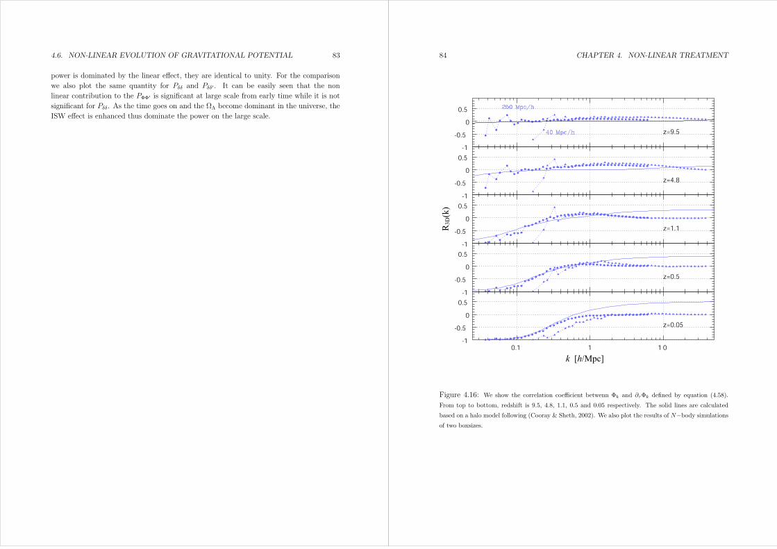
4.6. NON-LINEAR EVOLUTION OF GRAVITATIONAL POTENTIAL 83
power is dominated by the linear effect, they are identical to unity. For the comparison
we also plot the same quantity for Pδδ and Pδδ′ . It can be easily seen that the non
linear contribution to the PΦΦ′ is significant at large scale from early time while it is not
significant for Pδδ. As the time goes on and the ΩΛ become dominant in the universe, the
ISW effect is enhanced thus dominate the power on the large scale.
84 CHAPTER 4. NON-LINEAR TREATMENT
-1
-0.5
0
0.5
z=9.5
-1
-0.5
0
0.5
z=4.8
-1
-0.5
0
0.5
z=1.1
-1
-0.5
0
0.5
z=0.5
0.1 1 1 0-1
-0.5
0
0.5
z=0.05
k [h/Mpc]
R3
D(k
)
Figure 4.16: We show the correlation coefficient betwenn Φk and ∂τΦk defined by equation (4.58).
From top to bottom, redshift is 9.5, 4.8, 1.1, 0.5 and 0.05 respectively. The solid lines are calculated
based on a halo model following (Cooray & Sheth, 2002). We also plot the results of N−body simulationsof two boxsizes.
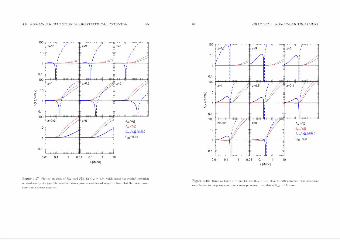
4.6. NON-LINEAR EVOLUTION OF GRAVITATIONAL POTENTIAL 85
0.1
1
10
100z=10 z=9 z=5
0.1
1
10
100z=1 z=0.5 z=0.1
0.01 0.1 1
0.1
1
10
100z=0.01
0.01 0.1 1 10
z=0
k [/Mpc]
Figure 4.17: Plotted are ratio of PΦΦ′ and P linΦΦ′ for ΩΛ0 = 0.74 which means the redshift evolution
of non-linearity of PΦΦ′ . The solid line shows positive and dashed negative. Note that the linear power
spectrum is always negative.
86 CHAPTER 4. NON-LINEAR TREATMENT
0.1
1
10
100z=10 z=9 z=5
0.1
1
10
100z=1 z=0.5 z=0.1
0.01 0.1 1
0.1
1
10
100z=0.01
0.01 0.1 1 10
z=0
k [/Mpc]
Figure 4.18: Same as figure 4.18 but for the ΩΛ0 = 0.1, close to EdS universe. The non-linear
contribution to the power spectrum is more prominent than that of ΩΛ0 = 0.74 case.
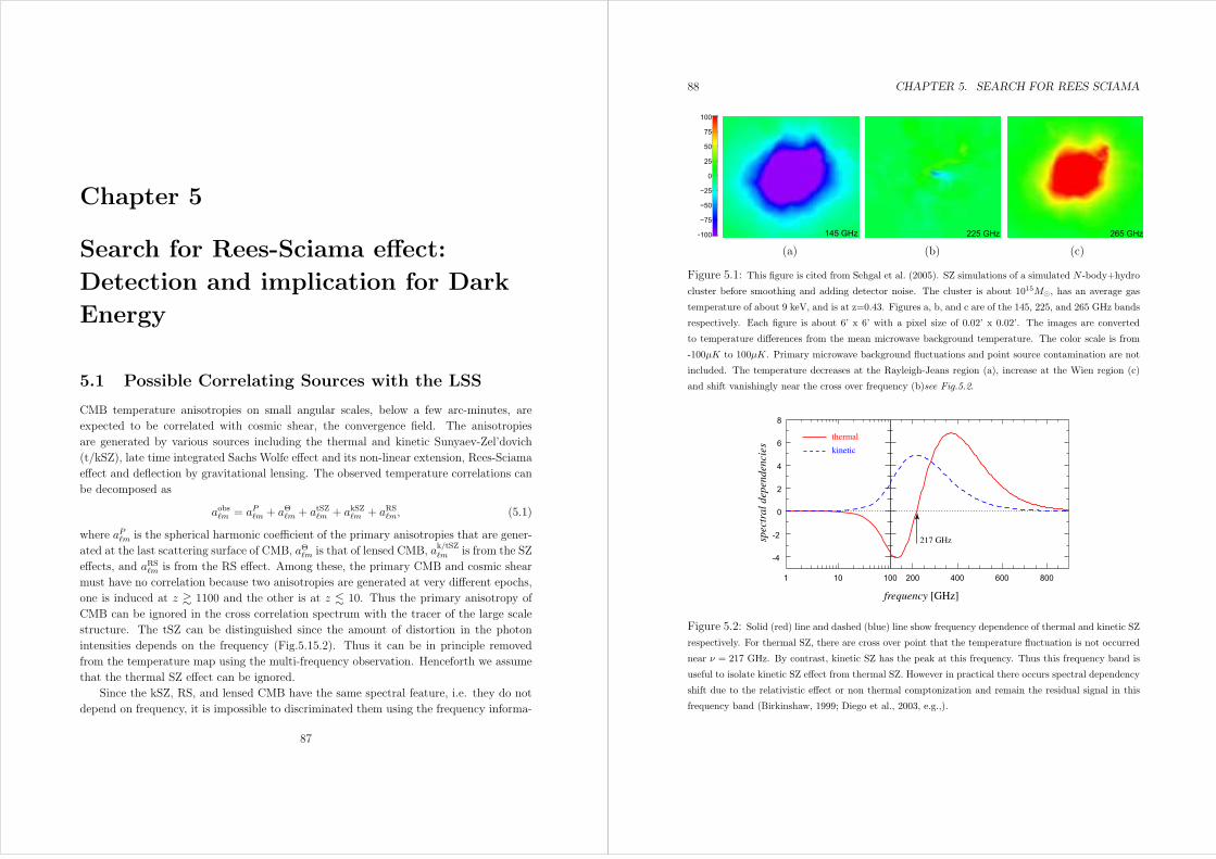
Chapter 5
Search for Rees-Sciama effect:
Detection and implication for Dark
Energy
5.1 Possible Correlating Sources with the LSS
CMB temperature anisotropies on small angular scales, below a few arc-minutes, are
expected to be correlated with cosmic shear, the convergence field. The anisotropies
are generated by various sources including the thermal and kinetic Sunyaev-Zel’dovich
(t/kSZ), late time integrated Sachs Wolfe effect and its non-linear extension, Rees-Sciama
effect and deflection by gravitational lensing. The observed temperature correlations can
be decomposed as
aobsm = aPm + aΘm + atSZm + akSZm + aRSm, (5.1)
where aPm is the spherical harmonic coefficient of the primary anisotropies that are gener-
ated at the last scattering surface of CMB, aΘm is that of lensed CMB, ak/tSZm is from the SZ
effects, and aRSm is from the RS effect. Among these, the primary CMB and cosmic shear
must have no correlation because two anisotropies are generated at very different epochs,
one is induced at z 1100 and the other is at z 10. Thus the primary anisotropy of
CMB can be ignored in the cross correlation spectrum with the tracer of the large scale
structure. The tSZ can be distinguished since the amount of distortion in the photon
intensities depends on the frequency (Fig.5.15.2). Thus it can be in principle removed
from the temperature map using the multi-frequency observation. Henceforth we assume
that the thermal SZ effect can be ignored.
Since the kSZ, RS, and lensed CMB have the same spectral feature, i.e. they do not
depend on frequency, it is impossible to discriminated them using the frequency informa-
87
88 CHAPTER 5. SEARCH FOR REES SCIAMA
−100
−75
−50
−25
0
25
50
75
100
145 GHz 225 GHz 265 GHz
(a) (b) (c)
Figure 5.1: This figure is cited from Sehgal et al. (2005). SZ simulations of a simulated N -body+hydro
cluster before smoothing and adding detector noise. The cluster is about 1015M, has an average gas
temperature of about 9 keV, and is at z=0.43. Figures a, b, and c are of the 145, 225, and 265 GHz bands
respectively. Each figure is about 6’ x 6’ with a pixel size of 0.02’ x 0.02’. The images are converted
to temperature differences from the mean microwave background temperature. The color scale is from
-100µK to 100µK. Primary microwave background fluctuations and point source contamination are not
included. The temperature decreases at the Rayleigh-Jeans region (a), increase at the Wien region (c)
and shift vanishingly near the cross over frequency (b)see Fig.5.2.
1 10 100
-4
-2
0
2
4
6
8
200 400 600 800
frequency [GHz]
spec
tral
dep
enden
cies
thermal
kinetic
217 GHz
Figure 5.2: Solid (red) line and dashed (blue) line show frequency dependence of thermal and kinetic SZ
respectively. For thermal SZ, there are cross over point that the temperature fluctuation is not occurred
near ν = 217 GHz. By contrast, kinetic SZ has the peak at this frequency. Thus this frequency band is
useful to isolate kinetic SZ effect from thermal SZ. However in practical there occurs spectral dependency
shift due to the relativistic effect or non thermal comptonization and remain the residual signal in this
frequency band (Birkinshaw, 1999; Diego et al., 2003, e.g.,).

5.1. POSSIBLE CORRELATING SOURCES WITH THE LSS 89
tion as like tSZ. However, in the linear regime, the kSZ effect and the mass distribution are
not correlated because peculiar velocities of clusters detached from the Hubble flow are
random in their directions along the line-of-sight. However the non-linear cross-correlation
between the kSZ effect and the convergence must be correlated and is calculated by Dore
et al. (2004). They found that the amplitude of correlation is rather small, at most
∆T/T 10−14. As we show below, the RS-κ cross-correlation is much larger, by about
two orders of magnitudes over the whole range of angular scales we consider.
The remaining source of correlation to be considered is lensed CMB. The spherical
harmonic coefficients for the lensed CMB are given by Komatsu & Spergel (2001)
aΘm =∑′m′
∑′′m′′
(−1)m+m′+m′′G−mm′m′′′′′ (5.2)
× ′(′ + 1)− (+ 1) + ′′(′′ + 1)2
aP∗′−m′Θ∗
′′−m′′ ,
where, Θm is the spherical harmonic transform of the deflection angle, Θ,
Θ(n) = −2∫ r∗
0
drr∗ − r
rr∗Φ(nr, r), (5.3)
which is expressed explicitly as
Θm = −8π(−i)∫
d3k
(2π)3Y ∗m(k)
∫ r∗
0
drr∗ − r
rr∗Φk(r)j(kr), (5.4)
with G−mm′m′′′′′ in equation (5.2) being the Gaunt integral given by equation(2.65). This
equation implies that 〈aΘmaκm〉 becomes third order moment and exactly vanishes for theGaussian field. Although there should be some non-Gaussian features in Φ (Zaldarriaga,
2000; Zaldarriaga & Seljak, 1999), the amplitude of the correlation between the lensed
CMB temperature and κ is induced purely non-Gaussianity thus would be thought to
be quite small. In summary, the CMB-κ correlation at small angular scales is likely to
be dominated by the RS-κ correlation. However the strict estimates of the amount of
correlation of κ and lensed CMB is left for the future work.
Note that Θm is related to aκm(z∗) by
aκlm(z∗) = −(+ 1)
2Θm (5.5)
which gives
aκm(z∗) = 4π(+ 1)(−i)∫
d3k
(2π)3Y ∗m(k)
∫ r∗
0
drr∗ − r
rr∗Φk(r)j(kr). (5.6)
90 CHAPTER 5. SEARCH FOR REES SCIAMA
This expression agrees with equation (5.13b) when z∗ → zs and ( + 1) → (kr)2. The
latter substitution is known as the ”flat-sky approximation” (Hu, 2000b). It is then easy
to show that for 1
〈aRSmΘ∗lm〉 = 2
∫ rs
0
drrs − r
r3rs
∂PΦ(k; r)
∂r
∣∣∣∣k=/r
, (5.7)
which agrees with equation (10) of Verde & Spergel (2002).
5.2 Angular Correlation Function
The CMB temperature anisotropies induced by a time-varying gravitational potential is
given by
∆T (n)
T= −2
∫ r∗
r0
dr∂
∂rΦ[nSK(r), r], (5.8)
where n is a two dimensional unit direction vector, and r is the conformal lookback time,
with r0 and r∗ denoting the present time and the surface of last scattering, respectively.The distribution of total matter can be probed by gravitational lensing observations.
A useful quantity is the convergence, κ, that is essentially the projection of matter density
along a line-of-sight,
κ(n; zs) =3ΩmH
20
2
∫ rs
0
drSK(r)SK(rs − r)
SK(rs)
δ[SK(r)n; r]
a, (5.9)
where rs ≡ r(zs) is the comoving distance out to a source at z = zs (Bartelmann et al.,
2001). Note that the angular diameter distance is equal to the comoving distance for a
spatially flat Universe, so we can reduce the above expression to simpler form,
κ(n; zs) =3ΩmH
20
2
∫ rs
0
drr(rs − r)
rs
δ(rn; r)
a, (5.10)
To take into consideration a distribution of sources at various redshifts contributing to the
weak gravitational lensing, we convolve equation (5.9) with a source distribution function,
n(zs),
κ(n) =
∫ z∗
0
dzs n(zs)κ(n; zs). (5.11)
The distribution function is normalized such that its integration over redshifts equals
unity. Working in a harmonic space simplify the analysis below. We first expand equa-

5.2. ANGULAR CORRELATION FUNCTION 91
tion (5.8) and (5.10) using the spherical harmonics:
∆TRS(n)
T=
∑,m
aRSmYm(n), (5.12a)
κ(n) =∑,m
aκmYm(n) (5.12b)
with
aRSm = 8π(−i)l∫
d3k
(2π)3Y ∗m(k)
∫ r∗
0
dr∂Φk
∂rjl(kr), (5.13a)
aκm(zs) = 4π(−i)∫
d3k
(2π)3k2Y ∗
m(k)
∫ rs
0
drr(rs − r)
rsΦk(r)j(kr). (5.13b)
Φk is Fourier counterpart of gravitational potential and the power spectrum of Φk is
related to Pδ(k, r) by
PΦ(k, r) =9Ω2m4
H40
k4Pδ(k, r)
a2(r). (5.14)
The cross-correlation power spectrum is then obtained to be
CRS−κ (zs) =
⟨aRSma
κ∗m(zs)
⟩(5.15)
=4
π
∫dk k4
∫ r∗
0
dr
∫ rs
0
dr′r′(rs − r′)
rsPΦΦ′(k; r, r′)j(kr)j(kr′),
where we have used the orthonormality relation of Ym(k), and a relation⟨∂Φk(r)
∂rΦk′(r′)
⟩:= (2π)3PΦΦ′(k; r, r′)δD(k− k′). (5.16)
Finally, we use the Limber’s approximation (Limber, 1954; Afshordi et al., 2004),
2
π
∫dk k4PΦΦ′(k; r, r′)j(kr)j(kr′) (5.17)
≈ l2
r4PΦΦ′
(k =
r; r
)δD(r − r′),
where δD is a Dirac Delta function. The cross-correlation power spectrum is then simpli-
fied to be
CRS−κ (zs) = 22
∫ rs
0
drrs − r
r3rsPΦΦ′(k; r)|k=/r . (5.18)
92 CHAPTER 5. SEARCH FOR REES SCIAMA
Figure 5.3: Two models of weak lensing survey. The Model 1 has its peak at very high redshift but
galaxies are lying over the wide range of redshift thus tend to mix wide range of scale for a given multipole.
The model 2 has its steeper peak at relatively lower redshift thus likely to isolate the scale at peak redshift
for a given multipole.
We compute the total cross-correlation, CRS−κ , by integrating equation (5.18) with a
wight of source distribution for a given weak-lensing survey,
CRS−κ =
∫ z∗
0
dzs n(zs)CRS−κ (zs). (5.19)
We refer CCAPS(Cross Correlation Angular Power Spectrum) to CRS−κ henceforth. As in
the literature, the radial distribution of source galaxies can be parametrized as (Efstathiou
et al., 1991),
n(z) = Az2 exp[−(z/z0)β] (5.20)
The values for realistic observation designs are provided by Semboloni et al. (2006) for
CFHTLS and Hennawi & Spergel (2005) for LSST. The normalization factor A is deter-
mined by integrating∫ ∞0
n(z)dz = 1. Thus the distribution n(z)dz can be thought as a
probability of finding the galaxy between z and z + dz. Another parametrization can be
found in the reference (e.g., Hu & Scranton, 2004). For the definiteness we adopted the
two models, (Model 1) Deep Survey, (β, z0) = (0.7, 0.5), whose n(z) peaks at z ∼ 2.2 with
a broad distribution, and (Model 2) Shallow Survey, (β, z0) = (2, 0.9), which peaks at
z 0.9 with a narrower distribution. Figure 5.3 shows normalized distribution function.
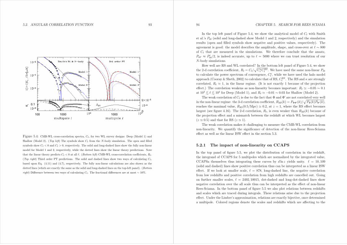
5.2. ANGULAR CORRELATION FUNCTION 93
100 1000
0.1
10000
Figure 5.4: CMB-WL cross-correlation spectra, C, for two WL survey designs: Deep (Model 1) and
Shallow (Model 2). (Top left) The symbols show C from the N -body simulation. The open and filled
symbols show C < 0 and C > 0, respectively. The solid and long-dashed lines show the fully non-linear
model for Model 1 and 2, respectively, while the dotted lines show the linear theory predictions. Note
that the linear theory predicts C < 0 at all . (Bottom left) CMB-WL cross-correlation coefficients, R.
(Top right) Third order PT predictions. The solid and dashed lines show two ways of calculating C,
based upon Eq. (4.11) and (4.7), respectively. The fully non-linear calculations are also shown as the
dotted lines (which are exactly the same as the solid and long-dashed lines on the top-left panel). (Bottom
right) Difference between two ways of calculating C. The fractional differences are at most ∼ 10%.
94 CHAPTER 5. SEARCH FOR REES SCIAMA
In the top left panel of Figure 5.4, we show the analytical model of C with Smith
et al.’s Pδδ (solid and long-dashed show Model 1 and 2, respectively) and the simulation
results (open and filled symbols show negative and positive values, respectively). The
agreement is good: the model describes the amplitude, shape, and cross-over at ∼ 800
of C that are measured in the simulations. We therefore conclude that the ansatz,
Pδδ′ ≈ P ′δδ/2, is indeed accurate, up to = 5000 where we can trust resolution of our
N -body simulations.
How well are RS and WL correlated? In the bottom left panel of Figure 5.4, we show
the 2-d correlation coefficient, R = C/√Cκ C
RS . We have used the same non-linear Pδδ
to calculate the power spectrum of convergence, Cκ , while we have used the halo model
approach (Cooray & Sheth, 2002) to calculate that of RS, CRS . The RS and κ are strongly
correlated, R 1, in the linear regime. (It is not exactly 1 because of the projection
effect.) The correlation weakens as non-linearity becomes important: R −0.05 ∼ 0.1
at 103 104 for Deep (Model 1), and R −0.01 ∼ 0.03 for Shallow (Model 2).
The weak correlation of C is due to the fact that Φ and Φ′ are not correlated very well
in the non-linear regime: the 3-d correlation coefficient, R3D(k) = PΦΦ′(k)/√PΦ(k)PΦ′(k),
reaches the maximal value, R3D(0.5/Mpc) 0.2, at z = 1, where the RS effect becomes
largest (see figure 4.16). The 2-d correlation, R, is even weaker than R3D(k) because of
the projection effect and a mismatch between the redshift at which WL becomes largest
(z 0.5) and that for RS (z 1).
The weak correlation makes it challenging to measure the CMB-WL correlation from
non-linearity. We quantify the significance of detection of the non-linear Rees-Sciama
effect as well as the linear ISW effect in the section 5.3.
5.2.1 The impact of non-linearity on CCAPS
In the top panel of figure 5.5, we plot the distribution of correlation in the redshift,
the integrand of CCAPS for 5 multipoles which are normalized by the integrated value,
CCAPSa themselves thus integrating these curves by d ln z yields unity. = 10, 109
(solid and dashed) lines show positive correlation thus can be interpreted as a linear ISW
effect. If we look at smaller scale, = 878, long-dashed line, the negative correlation
from low redshifts and positive correlation from high redshifts are cancelled out. Going
on further smaller scales, = 2492, 10015, dot-dashed and long-dot-dashed lines show
negative correlation over the all scale thus can be interpreted as the effect of non-linear
Rees-Sciama. In the bottom panel of figure 5.5 we also plot relations between redshifts
and scales which are traced during integrals. These relations arise due to the projection
effect. Under the Limber’s approximation, relations are exactly bijective, once determined
a multipole. Colored regions denote the scales and redshifts which are affecting to the

5.3. DETECTING THE SIGNATURE OF THE REES–SCIAMA EFFECT 95
total correlation. The widths are determined such that the correlation signal becomes
one third of its peak. Also shown are confidence region within which the commutativity
assumption is valid with blue and red solid lines labeled 10% and 1% respectively. Regions
below those lines are valid with fractional difference being 10% and 1%.
We can conclude that when we calculate cross correlation angular power spectrum
between convergence and Rees Sciama effect, we can use the fitting formular differenciated
with respect to time with accuracy being better than 1% for 2500 and 10% for 104
though the commutativity is invalid on deeply non-linear regime.
5.3 Detecting the signature of the Rees–Sciama Ef-
fect
In the section 5.1, we showed that the RS effect is the dominant source of temperature
anisotropy that contributes to the CMB-κ cross-correlation. We thus need to evaluate the
amplitude of the correlation to see if it can be detected by forthcoming/ideal observations.
The significance of detection can be quantified by the signal to noise ratio. The signal to
noise ratio for cross correlation at each multipole can be expressed as,
(S
N
)2
fskyCov−1
(CRS−κ
)2(5.21)
Cov =CCMB Cκ
+(CRS−κ
)22+ 1
, (5.22)
where fsky is the fraction of sky which both CMB and weak lensing are observed. The
factor 2 + 1 of covariance matrix is coming from the fact that for each multipoles there
are 2+1 harmonic m modes of ams. C is the expected angular power spectrum which is
a sum of the true angular correlation power spectrum and a noise spectrum, C = C+N.
The noise spectra of CMB and convergence are modeled as in (Knox, 1995; Schneider,
2005):
NCMB = σ2pixθ
2fwhm exp[(+ 1)θfwhm/8 ln 2], (5.23)
Nκ = σ2γ/ngal (5.24)
where σpix is the sensitivity to CMB temperature fluctuations in units of background
temperature, θfwhm is the full width half maximum of the gaussian beam size, ngal is the
number density of galaxies observed by the weak lensing survey per unit steradian, and
σγ is the dispersion on the intrinsic ellipticities of lensed galaxies. There exist no Noise
spectrum for the cross correlation since all of the noises associated to each observations
96 CHAPTER 5. SEARCH FOR REES SCIAMA
k [
Mp
c-1
]dC
l /
dln
z /
|Cl|
redshift z
l=10015
l=2492
l=878l=109
l=10
1/3
10%1%
Figure 5.5: (Top) The distribution of correlation in the redshift, the integrand of CCAPS for 5 multi-
poles which are normalized by the integrated value, CCAPSa themselves thus integrating these curves by
d ln z yields unity. = 10, 109 (solid and dashed) lines show positive correlation thus can be interpreted
as a linear ISW effect. If we look at smaller scale, = 878, long-dashed line, the negative correlation
from low redshifts and positive correlation from high redshifts are cancelled out. Going on further smaller
scales, = 2492, 10015, dot-dashed and long-dot-dashed lines show negative correlation over the all scale
thus can be interpreted as the effect of non-linear Rees-Sciama. (Bottom) Plotted are relations between
redshifts and scale which are traced during integrals. These relations arise due to the projection effect.
Under the Limber’s approximation, relations are exactly bijective, once determined a multipole. Colored
regions denote the scales and redshifts which are affecting to the total correlation. The widths are deter-
mined such that the correlation signal becomes one third of its peak. Also shown are confidence region
within which the commutativity assumption is valid with blue and red solid lines labeled 10% and 1%
respectively. Regions below those lines are valid with fractional difference being 10% and 1%.

5.3. DETECTING THE SIGNATURE OF THE REES–SCIAMA EFFECT 97
PLANCK nl
ACT nl
Figure 5.6: We plot the cumulative signal-to-noise ratio against angular multipole. The solid line is
calculated from the Smith et al. fitting formula, and the dotted line is for the halo approach with an
assumed observational error. The dashed line is a case without observational errors; this is an ideal,
or the most optimistic case. We consider ACT for CMB and CFHTLS for WL (left), and PLANCK 3
channels for CMB and LSST for WL (right).
98 CHAPTER 5. SEARCH FOR REES SCIAMA
Table 5.1: SURVEY PARAMETERSModel 106σPIX θFWHM fsky σγ ng
(arcmin) (/arcmin2)
CFHTLS - - 2.4e-2 0.3 20
LSST - - 0.8 0.1 100
ACT 4.4 1.7 2.4e-2 - -
PLANCK 1.7/2/4.3 10.7/8/5.5 0.8 - -
are never correlated. It is worth noting that, while detection of the integrated Sachs-Wolfe
effect on the linear scale is hampered by cosmic variance, the signal-to-noise (SN) ratio of
the Rees–Sciama effect on the non-linear scale is largely determined by the instrumental
capabilities and shot noise as well as the fraction of sky (to be) observed.
The cumulative signal-to-noise ratio is written as the sum of the S/N at each multipole,
(S
N
)2
=max∑=min
(S
N
)2
. (5.25)
In Figure 5.6, we show the predicted cumulative S/N as a function of the maximum
multipole, max, for cosmic-variance limited CMB and WL (Deep and Shallow) surveys,
as well as for the forthcoming surveys: Planck correlated with LSST, and ACT correlated
with CFHTLS (Nishizawa et al.2007 ApJL submitted). The observational strategies are
summarized at table 5.1. For the Planck, we assumed three lowest channels of High
Frequency Instrument (HFI) detector, which are 100, 143 and 217 GHz.
We find that S/N is totally dominated by the linear contribution (dotted lines) at
3000, and then becomes dominated by the non-linear contribution (dashed lines) at
higher . All-sky CMB and WL surveys can yield S/N ∼ 50 (10) for Deep (Shallow)
WL Survey, whereas 1000 deg2 surveys can only yield S/N ∼ 7 (1). Once noise of the
forthcoming surveys is included, however, S/N from the non-linear contribution becomes
small compared to the linear contribution. For Planck+LSST we find S/N ∼ 1.5 for the
non-linear, and 6 for the linear. For ACT+CFHTLS we find S/N ∼ 0.1 for the non-
linear, and 0.7 for the linear. Therefore, we conclude that these forthcoming surveys are
not expected to yield significant detection of non-linear RS effect.
The right bottom panel of figure 5.7 shows signal to noise ratio squared at each
multipoles , C2Cov−1. Blue lines are those of cosmic variance limited surveys with all
sky(dashed line) and 1000 deg2 sky (solid line) to be observed. We assume the deep weak
lens survey, Model 1 for all sky survey and shallow weak lens survey, Model 2 as described
by equation (5.20). Red lines are same as blue lines with realistic observational error for

5.4. SENSITIVITIES TO THE DARK ENERGY 99
combinations of CFHTLS with ACT (solid) and LSST with Planck (dashed). As can be
seen from this figure, LSST with Planck almost reaches the cosmic variance limited survey
in large scales, thus the detection of linear ISW effect using cross-correlation with mass
distribution enters a phase of its limitation at the Planck era, a next decade. However,
on small scales, the signal to noise ratio is suppressed in particular by the detector noise
of CMB observation at 1000.
5.4 Sensitivities to the Dark Energy
As the linear ISW effect vanishes during the matter dominated era, it is sensitive to dark
energy (DE) (e.g., Boughn & Crittenden, 2004; Nolta et al., 2004; Afshordi et al., 2004).
The non-linear RS effect measures the structure growth, which is also sensitive to DE
(Verde & Spergel, 2002). The cross-over at ∼ 800, at which the linear and non-linear
contributions cancel, is particularly a unique probe of DE. This is one of the main findings
of this thesis.
5.4.1 CCAPS Behavior
It is interesting to see the CCAPS behaviors as the parameters of dark energy vary.
Figure 5.8 shows how the CCAPS behaves as the dark energy parameters are varied.
The top panel show the dependency on ΩΛ0. The left and right panel correspond to the
two weak lensing survey models mentioned above. Each lines from top to bottom are
ΩΛ0 = 0.95, 0.8, 0.74, 0.65, 0.5, 0.35, 0.2, 0.05. The lowest (red) curve is close to the EdS
universe thus the significant suppression of linear ISW can be seen. Whereas on the small
scale (high ) the large matter density aid the accelerating structure evolution thus causes
the larger Φ′ at the non-linear stage. This brings the enhancement of non-linear RS effect.As the ΩΛ0 increases, the linear ISW is boosted and the non-linear structure growth is
suppressed. Note that the cross-over point does not depend largely on the ΩΛ0. This is
the result of somewhat artificial effect, the flat universe assumption, which we will give
an explanation below.
Figure 5.9 show sensitivity of C to DE parameters: ∂C/∂ΩΛ0, ∂C/∂w0, and ∂C/∂w1.
We use a simple form of DE equation of state, w(a) = pΛ(a)/ρΛ(a), given by w(a) =
w0+w1(1− a), the Taylor expansion with respect to scale factor around today (e.g., Lin-
der, 2003). The fiducial values are set to w0 = −1 and w1 = 0, the cosmological constant
model. We find ∂C/∂w0 < 0 and ∂C/∂w1 < 0 at all and that ∂C/∂ΩΛ0 < 0 at almost
entire but has positive part at intermediate scale.
In Fig. 5.10, we illustrate this enigmatic behaviors with the schematic sketch. The
solid black line is the CCAPS for the fiducial cosmological model. If the dark energy
100 CHAPTER 5. SEARCH FOR REES SCIAMA
0.1
1
10
100
10 100 1000 10000
0.1
1
10
10 100 1000 10000
(dCl / dΩΛ)2 Cov-1
(dCl / dw0)2 Cov-1
(dCl / dw1)2 Cov-1
(Cl)2 Cov-1
multipole l multipole l
Figure 5.7: (right-bottom) Signal to noise ratio from each multipole: equation (5.25) before taking
sum over multipole. The combination of LSST and Planck likely reaches to cosmic variance limited on
large scales while it loses S/N significantly on smaller scales because of the finite angular resolution of
Planck. The blue solid line shows cosmic variance limited (CVL) survey with 1000 deg2 observation, and
corresponding weak lens survey is shallow one. The blue dashed line shows CVL with fsky = 1, and deep
weak lens survey. The red solid and dashed lines show the combination of CFHTLS with ACT and LSST
with Planck respectively. (left-top) Contributions to fisher matrix given by equation (5.27) from each
multipoles for ΩΛ0. All lines denotes same observational sets as in the right-bottom panel. (left-bottom)
Same as previous but for w0. All lines denotes same observational sets as in the right-bottom panel.
(right-top) Same as previous but for w1. All lines denotes same observational sets as in the right-bottom
panel.
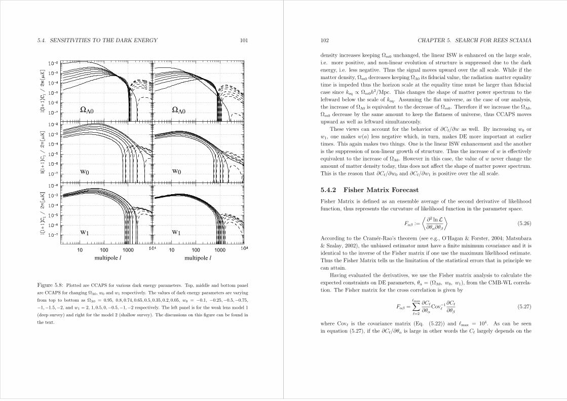
5.4. SENSITIVITIES TO THE DARK ENERGY 101
10 100 1000 10 100 1000multipole l multipole l
ΩΛ0 ΩΛ0
w0 w0
w1 w1
Figure 5.8: Plotted are CCAPS for various dark energy parameters. Top, middle and bottom panel
are CCAPS for changing ΩΛ0, w0 and w1 respectively. The values of dark energy parameters are varying
from top to bottom as ΩΛ0 = 0.95, 0.8, 0.74, 0.65, 0.5, 0.35, 0.2, 0.05, w0 = −0.1, −0.25,−0.5,−0.75,−1,−1.5,−2, and w1 = 2, 1, 0.5, 0,−0.5,−1,−2 respectively. The left panel is for the weak lens model 1(deep survey) and right for the model 2 (shallow survey). The discussions on this figure can be found in
the text.
102 CHAPTER 5. SEARCH FOR REES SCIAMA
density increases keeping Ωm0 unchanged, the linear ISW is enhanced on the large scale,
i.e. more positive, and non-linear evolution of structure is suppressed due to the dark
energy, i.e. less negative. Thus the signal moves upward over the all scale. While if the
matter density, Ωm0 decreases keeping ΩΛ0 its fiducial value, the radiation–matter equality
time is impeded thus the horizon scale at the equality time must be larger than fiducial
case since keq ∝ Ωm0h2/Mpc. This changes the shape of matter power spectrum to the
leftward below the scale of keq. Assuming the flat universe, as the case of our analysis,
the increase of ΩΛ0 is equivalent to the decrease of Ωm0. Therefore if we increase the ΩΛ0,
Ωm0 decrease by the same amount to keep the flatness of universe, thus CCAPS moves
upward as well as leftward simultaneously.
These views can account for the behavior of ∂C/∂w as well. By increasing w0 or
w1, one makes w(a) less negative which, in turn, makes DE more important at earlier
times. This again makes two things. One is the linear ISW enhancement and the another
is the suppression of non-linear growth of structure. Thus the increase of w is effectively
equivalent to the increase of ΩΛ0. However in this case, the value of w never change the
amount of matter density today, thus does not affect the shape of matter power spectrum.
This is the reason that ∂C/∂w0 and ∂C/∂w1 is positive over the all scale.
5.4.2 Fisher Matrix Forecast
Fisher Matrix is defined as an ensemble average of the second derivative of likelihood
function, thus represents the curvature of likelihood function in the parameter space.
Fαβ :=
⟨∂2 lnL∂θα∂θβ
⟩(5.26)
According to the Cramer-Rao’s theorem (see e.g., O’Hagan & Forster, 2004; Matsubara
& Szalay, 2002), the unbiased estimator must have a finite minimum covariance and it is
identical to the inverse of the Fisher matrix if one use the maximum likelihood estimate.
Thus the Fisher Matrix tells us the limitation of the statistical errors that in principle we
can attain.
Having evaluated the derivatives, we use the Fisher matrix analysis to calculate the
expected constraints on DE parameters, θα = (ΩΛ0, w0, w1), from the CMB-WL correla-
tion. The Fisher matrix for the cross correlation is given by
Fαβ =max∑=2
∂C
∂θαCov−1
∂C
∂θβ(5.27)
where Cov is the covariance matrix (Eq. (5.22)) and max = 104. As can be seen
in equation (5.27), if the ∂C/∂θα is large in other words the C largely depends on the

5.4. SENSITIVITIES TO THE DARK ENERGY 103
Figure 5.9: This figure shows the derivatives of CCAPS with respect to dark energy parameters, which
also imply the sensitivities of CCPAS to the dark energy parameters. The sign of these spectrum is
almost positive but has negative part at intermediate scale for ΩΛ0 and all positive for w0 and w1. The
dotted lines are predictions from linear theory. The first turn-up of ΩΛ0 appears also in the linear theory
thus it is a linear theory effect which we give a more detail in the text.
104 CHAPTER 5. SEARCH FOR REES SCIAMA
multipole l
ΩΛ increase
Ωm decrease
∆Ωm+∆ΩΛ = 0ISW boost
suppression of
structure formation
Horizon scale at
equality time
become larger
Figure 5.10: This is a schematic illustration how the CCAPS depends on the ΩΛ0. The solid black
line is the CCAPS for fiducial cosmological model. Red dotted line is that for the model with slightly
increased ΩΛ0 keeping Ωm0 unchanged. Blue dotted line is that for model with slightly decreased Ωm0
keeping ΩΛ0 at its fiducial value. If two are occurred at the same time, the resulting CCAPS can be
expected to be a dotted magenta line.
parameter θα, corresponding element of Fisher Matrix becomes large. Thus the constraint
on the θα is expected to be tight.
Figure 5.11 shows the expected 1σ constraints on w0 and w1 from cross correlation
Cl between ISW(+RS) and weak lensing. For left top panel, we assumed cosmic-variance
limited survey with shallow weak lensing galaxy distribution and the sky observed is 1000
deg2. Top right panel also shows constraints from cosmic-variance limited survey with
deep weak lensing galaxy distribution and the all-sky survey. In the bottom panel, we
plot the expected constraints from the forthcoming observational sets, CFHTLS with ACT
and LSST with Planck. For each panel, outer blue lines do not contain the non-linear RS
information. We use linear theory, do not include non-linear theory and set lmax to 300.
Inner red circles include non-linear RS effect and we chose lmax to 10000. If we extend lmaxfurther, we would gain more tight constraints on w0, w1 for the cosmic variance limited
survey, however there is a possibility that on further smaller scales, the kinetic SZ effect
might dominate the cross-correlation signal. Thus we truncate lmax at 10000. For all
panels, we fixed the value of ΩΛ0 to its fiducial value, 0.74 instead of marginalizing it.
When ΩΛ0 is fixed at the fiducial value, we find w0 = −1±1.1 (0.4) and w1 = 0±4.1 (1.1)for Shallow (Deep) WL Survey respectively. The constraints are not very strong however,
the direction of degeneracy line, w1 2(w0 + 1), is about twice as steep as that of Type
Ia supernovae observations (Seo & Eisenstein, 2003; Wood-Vasey et al., 2007). Thus it
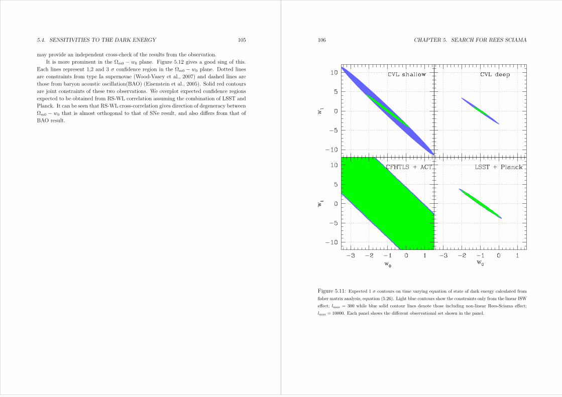
5.4. SENSITIVITIES TO THE DARK ENERGY 105
may provide an independent cross-check of the results from the observation.
It is more prominent in the Ωm0 − w0 plane. Figure 5.12 gives a good sing of this.
Each lines represent 1,2 and 3 σ confidence region in the Ωm0 − w0 plane. Dotted lines
are constraints from type Ia supernovae (Wood-Vasey et al., 2007) and dashed lines are
those from baryon acoustic oscillation(BAO) (Eisenstein et al., 2005). Solid red contours
are joint constraints of these two observations. We overplot expected confidence regions
expected to be obtained from RS-WL correlation assuming the combination of LSST and
Planck. It can be seen that RS-WL cross-correlation gives direction of degeneracy between
Ωm0 − w0 that is almost orthogonal to that of SNe result, and also differs from that of
BAO result.
106 CHAPTER 5. SEARCH FOR REES SCIAMA
Figure 5.11: Expected 1 σ contours on time varying equation of state of dark energy calculated from
fisher matrix analysis, equation (5.26). Light blue contours show the constraints only from the linear ISW
effect; lmax = 300 while blue solid contour lines denote those including non-linear Rees-Sciama effect;
lmax = 10000. Each panel shows the different observational set shown in the panel.
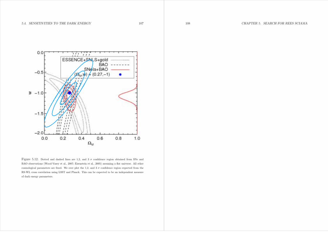
5.4. SENSITIVITIES TO THE DARK ENERGY 107
Figure 5.12: Dotted and dashed lines are 1,2, and 3 σ confidence region obtained from SNe and
BAO observations (Wood-Vasey et al., 2007; Eisenstein et al., 2005) assuming a flat universe. All other
cosmological parameters are fixed. We over plot the 1,2, and 3 σ confidence region expected from the
RS-WL cross correlation using LSST and Planck. This can be expected to be an independent measure
of dark energy parameters.
108 CHAPTER 5. SEARCH FOR REES SCIAMA

Chapter 6
Concluding Remark
We have studied the cross-correlation between the RS effect and the large scale matter
distribution traced by weak lensing convergence. The RS effect generates tiny tempera-
ture fluctuations of order ∆T/T 10−8. For this reason, cross-correlating it with massdistribution is more promising. The matter distribution differs from galaxy distribution
because of non-linear and/or scale dependent galaxy bias (e.g., Cole et al., 2005), and it
is non-trivial to infer the true mass distribution from the galaxy distribution. Thus we
use the weak lensing convergence, which directly traces the mass distribution along the
line of sight and thus free from the bias problem.
We have developed analytic models to calculate the cross-correlation at non-linear
scales. To this end, we assumed that the time derivative and average over k, the ensemble
average, are commutative up to fully non-linear scale. In other words, the differentiation
prescription is effective. This is valid in the linear theory because the time dependency
and scale dependency can be factorized. However, on the non-linear scale, the evolution
of fluctuation depends on scale and so the validity of the factorization is not obvious.
Several works on the RS effect in the context of the bispectrum (Goldberg & Spergel, 1999;
Spergel & Goldberg, 1999; Verde & Spergel, 2002) implicitly assume this commutativity
without explicitly proving. We have calculated the cross power spectrum using third order
perturbation theory by two different ways: differentiation prescription and momentum
one. The power spectrum obtained by these two method agree within 10% to the non-
linear scale. The obtained result supports the validity to take a time derivative of non-
linear power spectrum. However it remains unclear whether these two calculations are
consistently correct.
Then, in order to estimate the cross power spectrum, we use N -body simulations.
The results of simulations show remarkable agreement with the theoretical prediction
of differentiating the power spectrum obtained by Smith et al’s fitting formula, which
is more accurate than the third order PT in non-linear regime. We conclude that the
109
110 CHAPTER 6. CONCLUDING REMARK
differentiation prescription is valid over the all scales we traced by N -body simulations.
Moreover we have examined the detectability of the RS-κ cross-correlation by a com-
bination of forthcoming CMB and WL observations assuming an ideal observation set
for the cosmic variance limited survey. Overall, it appears rather difficult to establish
a significant detection because of large statistical noise. While next generation facilities
such as LSST and PLANCK are expected to detect non-linear RS effect with at most 2σ
confidence level, statistically we can achieve 50σ for an angular resolution of lmax = 10000.
The cross angular power spectrum shows negative sign, which means anti-correlation
between RS and κ on large scales, and positive sign on small scales. Thus there is a
cross over point at an intermediate scale 800. This scale is sensitive to the nature
of dark energy, in particular to equation of state of dark energy. We propose that the
scale can be used as a unique probe of dark energy. We found from the Fisher matrix
analysis that the expected constraints on w0–w1 is not so strong but the orientation
of degeneracy is twice steeper than that from the joint observation of baryon acoustic
oscillations and supernovae. It will provide an independent cross-check of the results
from these observations.

Bibliography
Afshordi, N., Loh, Y.-S., & Strauss, M. A. 2004, Phys.Rev.D, 69, 083524. “Cross-
correlation of the cosmic microwave background with the 2MASS galaxy survey: Sig-
natures of dark energy, hot gas, and point sources”
Ahn, M. H., et al. 2006, Phys.Rev.D, 74, 072003. “Measurement of neutrino oscillation
by the K2K experiment”
Athanassopoulos, C., et al. 1995, Physical Review Letters, 75, 2650. “Candidate events
in a search for νν –> νe oscillations”
Bardeen, J. M. 1980, Phys.Rev.D, 22, 1882. “Gauge-invariant cosmological perturbations”
Bardeen, J. M., Bond, J. R., Kaiser, N., & Szalay, A. S. 1986, ApJ, 304, 15. “The statistics
of peaks of Gaussian random fields”
Bartelmann, M., King, L. J., & Schneider, P. 2001, A&A, 378, 361. “Weak-lensing halo
numbers and dark-matter profiles”
Benitez, N., et al. 2002, in Bulletin of the American Astronomical Society, Vol. 34, Bulletin
of the American Astronomical Society, 1236
Bernardeau, F. 1994, ApJ, 433, 1. “Skewness and kurtosis in large-scale cosmic fields”
Bernardeau, F., Colombi, S., Gaztanaga, E., & Scoccimarro, R. 2002, Phys. Rep., 367, 1.
“Large-scale structure of the Universe and cosmological perturbation theory”
Birkinshaw, M. 1999, Phys. Rep., 310, 97. “The Sunyaev-Zel’dovich effect”
Bond, J. R., & Efstathiou, G. 1984, ApJ, 285, L45. “Cosmic background radiation
anisotropies in universes dominated by nonbaryonic dark matter”
Bond, J. R., Efstathiou, G., & Silk, J. 1980, Physical Review Letters, 45, 1980. “Massive
neutrinos and the large-scale structure of the universe”
111
112 BIBLIOGRAPHY
Bond, J. R., & Szalay, A. S. 1983, ApJ, 274, 443. “The collisionless damping of density
fluctuations in an expanding universe”
Bonnet, H., & Mellier, Y. 1995, A&A, 303, 331. “Statistical analysis of weak gravitational
shear in the extended periphery of rich galaxy clusters.”
Boughn, S., & Crittenden, R. 2004, Nature, 427, 45. “A correlation of the cosmic mi-
crowave sky with large scale structure”
Brandt, D., Burkhardt, H., Lamont, M., Myers, S., & Wenninger, J. 2000, Reports of
Progress in Physics, 63, 939. “Accelerator physics at LEP”
Carroll, S. M., Press, W. H., & Turner, E. L. 1992, ARA&A, 30, 499. “The cosmological
constant”
Cole, S., & Kaiser, N. 1989, MNRAS, 237, 1127. “Biased clustering in the cold dark
matter cosmogony”
Cole, S., & Lacey, C. 1996, MNRAS, 281, 716. “The structure of dark matter haloes in
hierarchical clustering models”
Cole, S., et al. 2005, MNRAS, 362, 505. “The 2dF Galaxy Redshift Survey: power-
spectrum analysis of the final data set and cosmological implications”
Colın, P., Klypin, A. A., Kravtsov, A. V., & Khokhlov, A. M. 1999, ApJ, 523, 32. “Evo-
lution of Bias in Different Cosmological Models”
Colombo, L. P. L., & Gervasi, M. 2006, Journal of Cosmology and Astro-Particle Physics,
10, 1. “Constraints on quintessence using recent cosmological data”
Cooray, A. 2002, Phys.Rev.D, 65, 083518. “Nonlinear integrated Sachs-Wolfe effect”
Cooray, A., & Sheth, R. K. 2002, Phys. Rept., 372, 1. “Halo models of large scale
structure”
Corasaniti, P. S., Kunz, M., Parkinson, D., Copeland, E. J., & Bassett, B. A. 2004,
Phys.Rev.D, 70, 083006. “Foundations of observing dark energy dynamics with the
Wilkinson Microwave Anisotropy Probe”
Curran, S. J., Darling, J., Bolatto, A. D., Whiting, M. T., Bignell, C., & Webb, J. K. 2007,
MNRAS, 382, L11. “HI and OH absorption in the lensing galaxy of MG J0414+0534”
BIBLIOGRAPHY 113
Diego, J. M., Hansen, S. H., & Silk, J. 2003, MNRAS, 338, 796. “The impact of relativistic
corrections and component separation in the measurement of the Sunyaev-Zel’dovich
effect and on the small angular scale non-Gaussianity of the cosmic microwave back-
ground”
Dore, O., Hennawi, J. F., & Spergel, D. N. 2004, ApJ, 606, 46. “Beyond the Damping
Tail: Cross-Correlating the Kinetic Sunyaev-Zel’dovich Effect with Cosmic Shear”
Dvali, G., Gruzinov, A., & Zaldarriaga, M. 2004, Phys.Rev.D, 69, 023505. “New mecha-
nism for generating density perturbations from inflation”
Efstathiou, G., Bernstein, G., Tyson, J. A., Katz, N., & Guhathakurta, P. 1991, ApJ,
380, L47. “The clustering of faint galaxies”
Efstathiou, G., & Bond, J. R. 1986, MNRAS, 218, 103. “Isocurvature cold dark matter
fluctuations”
Efstathiou, G., Bond, J. R., & White, S. D. M. 1992, MNRAS, 258, 1P. “COBE back-
ground radiation anisotropies and large-scale structure in the universe”
Efstathiou, G., Davis, M., White, S. D. M., & Frenk, C. S. 1985, ApJS, 57, 241. “Numer-
ical techniques for large cosmological N-body simulations”
Eisenstein, D. J., & Hu, W. 1998, ApJ, 496, 605. “Baryonic Features in the Matter
Transfer Function”
Eisenstein, D. J., & Hu, W. 1999, ApJ, 511, 5. “Power Spectra for Cold Dark Matter and
Its Variants”
Eisenstein, D. J., et al. 2005, ApJ, 633, 560. “Detection of the Baryon Acoustic Peak in
the Large-Scale Correlation Function of SDSS Luminous Red Galaxies”
Eke, V. R., Cole, S., & Frenk, C. S. 1996, MNRAS, 282, 263. “Cluster evolution as a
diagnostic for Omega”
Friedberg, R., & Martin, O. 1987, Journal of Physics A Mathematical General, 20, 5095.
“Fast evaluation of lattice Green functions ”
Fry, J. N. 1984, ApJ, 279, 499. “The Galaxy correlation hierarchy in perturbation theory”
Fukushige, T., & Makino, J. 1997, ApJ, 477, L9. “On the Origin of Cusps in Dark Matter
Halos”
114 BIBLIOGRAPHY
Goldberg, D. M., & Spergel, D. N. 1999, Phys.Rev.D, 59, 103002. “Microwave background
bispectrum. II. A probe of the low redshift universe”
Heath, D. J. 1977, MNRAS, 179, 351. “The growth of density perturbations in zero
pressure Friedmann-Lemaitre universes”
Hennawi, J. F., & Spergel, D. N. 2005, ApJ, 624, 59. “Shear-selected Cluster Cosmology:
Tomography and Optimal Filtering”
Henry, J. P. 2000, ApJ, 534, 565. “Measuring Cosmological Parameters from the Evolution
of Cluster X-Ray Temperatures”
Hernquist, L. 1990, ApJ, 356, 359. “An analytical model for spherical galaxies and bulges”
Hill, J. E. 1995, Physical Review Letters, 75, 2654. “An alternative analysis of the LSND
neutrino oscillation search data on νν –> νe”
Hockney, E., & Eastwood, M. 1981, Computer Simulation Using Particles (New York;
McGraw Hill)
Holtzman, J. A. 1989, ApJS, 71, 1. “Microwave background anisotropies and large-
scale structure in universes with cold dark matter, baryons, radiation, and massive and
massless neutrinos”
Hoyle, F., Outram, P. J., Shanks, T., Croom, S. M., Boyle, B. J., Loaring, N. S., Miller,
L., & Smith, R. J. 2002, MNRAS, 329, 336. “The 2dF QSO Redshift Survey - IV. The
QSO power spectrum from the 10k catalogue”
Hu, W. 2000a, ApJ, 529, 12. “Reionization Revisited: Secondary Cosmic Microwave
Background Anisotropies and Polarization”
Hu, W. 2000b, Phys.Rev.D, 62, 043007. “Weak Lensing of the CMB: A Harmonic Ap-
proach”
Hu, W., & Eisenstein, D. J. 1998, ApJ, 498, 497. “Small-Scale Perturbations in a General
Mixed Dark Matter Cosmology”
Hu, W., & Haiman, Z. 2003, Phys.Rev.D, 68, 063004. “Redshifting rings of power”
Hu, W., Scott, D., Sugiyama, N., & White, M. 1995, Phys.Rev.D, 52, 5498. “Effect of
physical assumptions on the calculation of microwave background anisotropies”
Hu, W., & Scranton, R. 2004, Phys.Rev.D, 70, 123002. “Measuring dark energy clustering
with CMB-galaxy correlations”

BIBLIOGRAPHY 115
Hu, W., & Sugiyama, N. 1996, ApJ, 471, 542. “Small-Scale Cosmological Perturbations:
an Analytic Approach”
Huss, A., Jain, B., & Steinmetz, M. 1999, ApJ, 517, 64. “How Universal Are the Density
Profiles of Dark Halos?”
Hutsi, G. 2006, A&A, 449, 891. “Acoustic oscillations in the SDSS DR4 luminous red
galaxy sample power spectrum”
Jain, B., & Bertschinger, E. 1994, ApJ, 431, 495. “Second-order power spectrum and
nonlinear evolution at high redshift”
Jain, B., & Seljak, U. 1997, ApJ, 484, 560. “Cosmological Model Predictions for Weak
Lensing: Linear and Nonlinear Regimes”
Jeong, D., & Komatsu, E. 2006, ApJ, 651, 619. “Perturbation Theory Reloaded: Ana-
lytical Calculation of Nonlinearity in Baryonic Oscillations in the Real-Space Matter
Power Spectrum”
Kaiser, N. 1998, ApJ, 498, 26. “Weak Lensing and Cosmology”
Knox, L. 1995, Phys.Rev.D, 52, 4307. “Determination of inflationary observables by
cosmic microwave background anisotropy experiments”
Kochanek, C. S. 1990, MNRAS, 247, 135. “Inverting Cluster Gravitational Lenses”
Kodama, H., & Sasaki, M. 1984, Progress of Theoretical Physics Supplement, 78, 1.
“Cosmological Perturbation Theory”
Kolb, E., & Turner, M. 1990, The Early Universe (Westview Press)
Komatsu, E., & Spergel, D. N. 2001, Phys.Rev.D, 63, 063002. “Acoustic signatures in
the primary microwave background bispectrum”
Kosowsky, A. 2003, New Astronomy Review, 47, 939. “The Atacama Cosmology Tele-
scope”
Lahav, O., Lilje, P. B., Primack, J. R., & Rees, M. J. 1991, MNRAS, 251, 128. “Dynamical
effects of the cosmological constant”
Lamarre, J. M., et al. 2003, New Astronomy Review, 47, 1017. “The Planck High Fre-
quency Instrument, a third generation CMB experiment, and a full sky submillimeter
survey”
116 BIBLIOGRAPHY
Lewis, A., & Bridle, S. 2002, Phys.Rev.D, 66, 103511. “Cosmological parameters from
CMB and other data: A Monte Carlo approach”
Limber, D. N. 1954, ApJ, 119, 655. “The Analysis of Counts of the Extragalactic Nebulae
in Terms of a Fluctuating Density Field. II.”
Linder, E. V. 2003, Physical Review Letters, 90, 091301. “Exploring the Expansion
History of the Universe”
Ma, C.-P., & Fry, J. N. 2000, ApJ, 543, 503. “Deriving the Nonlinear Cosmological
Power Spectrum and Bispectrum from Analytic Dark Matter Halo Profiles and Mass
Functions”
Magueijo, J. 2000, ApJ, 528, L57. “New Non-Gaussian Feature in COBE-DMR 4 Year
Maps”
Makino, N., Sasaki, M., & Suto, Y. 1992, Phys.Rev.D, 46, 585. “Analytic approach to the
perturbative expansion of nonlinear gravitational fluctuations in cosmological density
and velocity fields”
Marinucci, D. 2005, arXiv math, 0509430. “A Central Limit Theorem and Higher Order
Results for the Angular Bispectrum”
Martel, H., & Freudling, W. 1991, ApJ, 371, 1. “Second-order perturbation theory in
Omega is not equal to Friedmann models”
Mather, J. C., et al. 1994, ApJ, 420, 439. “Measurement of the cosmic microwave back-
ground spectrum by the COBE FIRAS instrument”
Mather, J. C., Fixsen, D. J., Shafer, R. A., Mosier, C., & Wilkinson, D. T. 1999, ApJ,
512, 511. “Calibrator Design for the COBE Far-Infrared Absolute Spectrophotometer
(FIRAS)”
Matsubara, T., & Szalay, A. S. 2002, ApJ, 574, 1. “Cosmological Parameters from
Redshift-Space Correlations”
Matsubara, T., & Szalay, A. S. 2003, Physical Review Letters, 90, 021302. “Apparent
Clustering of Intermediate-Redshift Galaxies as a Probe of Dark Energy”
Miralda-Escude, J. 1991, ApJ, 380, 1. “The correlation function of galaxy ellipticities
produced by gravitational lensing”
BIBLIOGRAPHY 117
Mo, H. J., & White, S. D. M. 1996, MNRAS, 282, 347. “An analytic model for the spatial
clustering of dark matter haloes”
Moore, B., Governato, F., Quinn, T., Stadel, J., & Lake, G. 1998, ApJ, 499, L5. “Resolv-
ing the Structure of Cold Dark Matter Halos”
Moore, B., Quinn, T., Governato, F., Stadel, J., & Lake, G. 1999, MNRAS, 310, 1147.
“Cold collapse and the core catastrophe”
Nakamura, T. T., & Suto, Y. 1997, Progress of Theoretical Physics, 97, 49. “Strong Grav-
itational Lensing and Velocity Function as Tools to Probe Cosmological Parameters —
Current Constraints and Future Predictions —”
Navarro, J. F., Frenk, C. S., & White, S. D. M. 1997, ApJ, 490, 493. “A Universal Density
Profile from Hierarchical Clustering”
Nishimichi, T., et al. 2007, ArXiv e-prints, 705. “Characteristic Scales of Baryon Acoustic
Oscillations from Perturbation Theory: Non-linearity and Redshift-Space Distortion
Effects”
Nolta, M. R., et al. 2004, ApJ, 608, 10. “First Year Wilkinson Microwave Anisotropy
Probe (WMAP) Observations: Dark Energy Induced Correlation with Radio Sources”
O’Hagan, A., & Forster, J. 2004, Kendall’s Advanced Theory of Statistics : Volume 2B :
Bayesian Inference (A Hodder Arnold Publication)
Okada, N., & Yasuda, O. 1997, International Journal of Modern Physics A, 12, 3669. “A
sterile neutrino scenario constrained by experiments and cosmology.”
Outram, P. J., Hoyle, F., Shanks, T., Croom, S. M., Boyle, B. J., Miller, L., Smith, R. J.,
& Myers, A. D. 2003, MNRAS, 342, 483. “The 2dF QSO Redshift Survey - XI. The
QSO power spectrum”
Padmanabhan, N., et al. 2007, MNRAS, 378, 852. “The clustering of luminous red galaxies
in the Sloan Digital Sky Survey imaging data”
Peacock, J. 1999, Cosmological Physics (Camblidge University Press)
Peacock, J. A. 2001, astro-ph/0105450. “Measuring large-scale structure with the 2dF
Galaxy Redshift Surveys”
Peacock, J. A., & Dodds, S. J. 1996, MNRAS, 280, L19. “Non-linear evolution of cosmo-
logical power spectra”
118 BIBLIOGRAPHY
Peebles, P. J. E. 1980, The Large-Scale Structure of the Universe (Princeton University
Press)
Peebles, P. J. E. 1982, ApJ, 263, L1. “Large-scale background temperature and mass
fluctuations due to scale-invariant primeval perturbations”
Percival, W. J. 2005, MNRAS, 356, 1168. “Markov chain reconstruction of the 2dF Galaxy
Redshift Survey real-space power spectrum”
Percival, W. J., et al. 2001, MNRAS, 327, 1297. “The 2dF Galaxy Redshift Survey: the
power spectrum and the matter content of the Universe”
Percival, W. J., Cole, S., Eisenstein, D. J., Nichol, R. C., Peacock, J. A., Pope, A. C., &
Szalay, A. S. 2007a, ArXiv e-prints, 705. “Measuring the Baryon Acoustic Oscillation
scale using the SDSS and 2dFGRS”
Percival, W. J., et al. 2007b, ApJ, 657, 645. “The Shape of the Sloan Digital Sky Survey
Data Release 5 Galaxy Power Spectrum”
Percival, W. J., et al. 2002, MNRAS, 337, 1068. “Parameter constraints for flat cosmolo-
gies from cosmic microwave background and 2dFGRS power spectra”
Perlmutter, S., et al. 1999, ApJ, 517, 565. “Measurements of Omega and Lambda from
42 High-Redshift Supernovae”
Press, W. H., & Schechter, P. 1974, ApJ, 187, 425. “Formation of Galaxies and Clusters
of Galaxies by Self-Similar Gravitational Condensation”
Rees, M. J., & Sciama, D. W. 1968, Nature, 217, 511. “Larger scale Density Inhomo-
geneities in the Universe”
Ruhl, J., et al. 2004, in Presented at the Society of Photo-Optical Instrumentation En-
gineers (SPIE) Conference, Vol. 5498, Millimeter and Submillimeter Detectors for As-
tronomy II. Edited by Jonas Zmuidzinas, Wayne S. Holland and Stafford Withington
Proceedings of the SPIE, Volume 5498, pp. 11-29 (2004)., ed. C. M. Bradford, P. A. R.
Ade, J. E. Aguirre, J. J. Bock, M. Dragovan, L. Duband, L. Earle, J. Glenn, H. Mat-
suhara, B. J. Naylor, H. T. Nguyen, M. Yun, & J. Zmuidzinas, 11
Sachs, R. K., & Wolfe, A. M. 1967, ApJ, 147, 73. “Perturbations of a Cosmological Model
and Angular Variations of the Microwave Background”
Sakurai, J. J. 1994, Modern Quantum Mechanics (Addison-Wesley)
BIBLIOGRAPHY 119
Sanchez, A. G., Baugh, C. M., Percival, W. J., Peacock, J. A., Padilla, N. D., Cole, S.,
Frenk, C. S., & Norberg, P. 2006, MNRAS, 366, 189. “Cosmological parameters from
cosmic microwave background measurements and the final 2dF Galaxy Redshift Survey
power spectrum”
Sanchez, A. G., & Cole, S. 2007, arXive:astro-ph, 0708.1517. “The galaxy power spectrum:
precision cosmology from large scale structure?”
Scherrer, R. J., & Bertschinger, E. 1991, ApJ, 381, 349. “Statistics of primordial density
perturbations from discrete seed masses”
Schneider, P. 2005, astro-ph, 0509252. “Weak Gravitational Lensing”
Schneider, P., et al. 1999, Gravitational Lenses (Springer Verlag)
Schneider, P., & Seitz, C. 1995, A&A, 294, 411. “Steps towards nonlinear cluster inversion
through gravitational distortions. 1: Basic considerations and circular clusters”
Schneider, P., van Waerbeke, L., Jain, B., & Kruse, G. 1998, MNRAS, 296, 873. “A new
measure for cosmic shear”
Sehgal, N., Kosowsky, A., & Holder, G. 2005, ApJ, 635, 22. “Constrained Cluster Pa-
rameters from Sunyaev-Zel’dovich Observations”
Seitz, C., & Schneider, P. 1997, A&A, 318, 687. “Steps towards nonlinear cluster inversion
through gravitational distortions. III. Including a redshift distribution of the sources.”
Seljak, U. 1996, ApJ, 460, 549. “Rees-Sciama Effect in a Cold Dark Matter Universe”
Seljak, U. 2000, MNRAS, 318, 203. “Analytic model for galaxy and dark matter cluster-
ing”
Seljak, U., & Zaldarriaga, M. 1996, ApJ, 469, 437. “A Line-of-Sight Integration Approach
to Cosmic Microwave Background Anisotropies”
Semboloni, E., et al. 2006, A&A, 452, 51. “Cosmic shear analysis with CFHTLS deep
data”
Seo, H.-J., & Eisenstein, D. J. 2003, ApJ, 598, 720. “Probing Dark Energy with Baryonic
Acoustic Oscillations from Future Large Galaxy Redshift Surveys”
Sheth, R. K., & Diaferio, A. 2001, MNRAS, 322, 901. “Peculiar velocities of galaxies and
clusters”
120 BIBLIOGRAPHY
Sheth, R. K., Hui, L., Diaferio, A., & Scoccimarro, R. 2001, MNRAS, 325, 1288. “Linear
and non-linear contributions to pairwise peculiar velocities”
Sheth, R. K., & Tormen, G. 1999, MNRAS, 308, 119. “Large-scale bias and the peak
background split”
Smith, R. E., et al. 2003, MNRAS, 341, 1311. “Stable clustering, the halo model and
non-linear cosmological power spectra”
Smoot, G. F., et al. 1992, ApJ, 396, L1. “Structure in the COBE differential microwave
radiometer first-year maps”
Spergel, D. N., et al. 2007, ApJS, 170, 377. “Wilkinson Microwave Anisotropy Probe
(WMAP) three year results: Implications for cosmology”
Spergel, D. N., & Goldberg, D. M. 1999, Phys.Rev.D, 59, 103001. “Microwave background
bispectrum. I. Basic formalism”
Spergel, D. N., et al. 2003, ApJS, 148, 175. “First-Year Wilkinson Microwave Anisotropy
Probe (WMAP) Observations: Determination of Cosmological Parameters”
Springel, V. 2005, MNRAS, 364, 1105. “The cosmological simulation code GADGET-2”
Sunyaev, R. A., & Zeldovich, I. B. 1980, MNRAS, 190, 413. “The velocity of clusters of
galaxies relative to the microwave background - The possibility of its measurement”
Suto, Y., & Sasaki, M. 1991, Physical Review Letters, 66, 264. “Quasinonlinear theory
of cosmological self-gravitating systems”
Tegmark, M., et al. 2004, ApJ, 606, 702. “The Three-Dimensional Power Spectrum of
Galaxies from the Sloan Digital Sky Survey”
Tegmark, M., et al. 2006, Phys.Rev.D, 74, 123507. “Cosmological constraints from the
SDSS luminous red galaxies”
Tegmark, M., Hamilton, A. J. S., & Xu, Y. 2002, MNRAS, 335, 887. “The power spectrum
of galaxies in the 2dF 100k redshift survey”
Tormen, G., Bouchet, F. R., & White, S. D. M. 1997, MNRAS, 286, 865. “The structure
and dynamical evolution of dark matter haloes”
Tuluie, R., Laguna, P., & Anninos, P. 1996, ApJ, 463, 15. “Cosmic Microwave Background
Anisotropies from the Rees-Sciama Effect in Ω0 ≤ 1 Universes”
BIBLIOGRAPHY 121
Verde, L., & Spergel, D. N. 2002, Phys.Rev.D, 65, 043007. “Dark energy and cosmic
microwave background bispectrum”
Viel, M., Lesgourgues, J., Haehnelt, M. G., Matarrese, S., & Riotto, A. 2005, Phys.Rev.D,
71, 063534. “Constraining warm dark matter candidates including sterile neutrinos and
light gravitinos with WMAP and the Lyman-α forest”
Wang, L., & Kamionkowski, M. 2000, Phys.Rev.D, 61, 063504. “Cosmic microwave back-
ground bispectrum and inflation”
Wood-Vasey, W. M., et al. 2007, ApJ, 666, 694. “Observational Constraints on the Nature
of Dark Energy: First Cosmological Results from the ESSENCE Supernova Survey”
Zaldarriaga, M. 2000, Phys.Rev.D, 62, 063510. “Lensing of the CMB: Non-Gaussian
aspects”
Zaldarriaga, M., & Seljak, U. 1999, Phys.Rev.D, 59, 123507. “Reconstructing projected
matter density power spectrum from cosmic microwave background”
122 BIBLIOGRAPHY
Appendix A
Fitting Formulae of Transfer
Function
In this appendix, I summarize fitting formulae of transfer function.
A.1 Peebles 1982
The fitting formula of transfer function is first developed by (Peebles, 1982)
T (k) = (1 + αk + βk2)−1 (A.1)
with α = 6(Θ2.7/h)2Mpc, β = 2.65(Θ2.7/h)
4Mpc2. Θ2.7 is CMB temperature in the unit
of 2.7K.
A.2 Bond Efstathiou 1984
Bond & Efstathiou (1984) and Efstathiou et al. (1992) improve this formula as
T (k) =1 +
[ak + (bk)3/2 + (ck)2
]ν−1/ν(A.2)
with the best fit values, a = (6.4/Γ)h−1Mpc, b = (3/Γ)h−1Mpc, c = (1.7/Γ)h−1Mpc,ν = 1.13 respectively when measuring k in the unit of hMpc−1. In the Einstein de Sitteruniverse, Ωm0 = 1, this fitting function is very accurate, and even in the flat ΛCDM
universe, it remains reasonable. CDM with decaying neutrino with mass 10m10[keV] and
lifetime τd [yr] change the shape parameter as Γ = Ωm0h/[0.861 + 3.8(m10τd)3/2]1/2 and
equation (A.2) is still reasonable.
123
124 APPENDIX A. TRANSFER FUNCTION
A.3 BBKS 1986
Bardeen et al. (1986) provides the another fitting formula drawn from the works (Bond &
Szalay, 1983; Bond & Efstathiou, 1984; Efstathiou & Bond, 1986) classified into 4 types
of situation by the condition of perturbation and species. I refer here only for 2 cases,
CDM and neutrino dark matter without entropy fluctuations.
Case I : Cold Dark Matter
TCDM,DM(k) =ln(1 + 2.34q)
2.34q[1 + 3.89q + (16.1q)2 + (5.46q)3 + (6.71q)4]−1/4 (A.3)
q :=k
Γ hMpc−1(A.4)
for the case that there exists, as a relativistic particles, only neutrino whose flavor
is three and photon. For the baryon, transfer function is filtered due to the acoustic
oscillation,
TCDM,B(k) = TCDM,DM(k)[1 + (kRJ)2/2]−1, (A.5)
where RJ = 1.6/√Ωm0 h
−1kpc is the Jeans scale. For the ΩB, being not small, Bond
& Efstathiou (1984) also gives similar fitting formula for the baryon.
Case II : One species Massive Neutrino Dark Matter
Tν,ad(k) = exp[−0.16(kRf )− (kRf )2/2][1 + 1.6q + (4.0q)3/2 + (0.92q)2]−1, (A.6)
where
q :=k
Γν hMpc−1, Rf = 2.6(Γν)
−1 h−1Mpc. (A.7)
Γν := Ωνh is shape parameter for Massive Neutrino dark matter, and Rf is trans-
lated as characteristic scale of neutrino free streaming below which power spec-
trum causes dumping exponentially. Note that physical amount of neutrino Ωνh2 =
0.31mν/(30eV).
A.4 Eisenstein & Hu 1998
Eisenstein & Hu (1998) takes small scale physics more carefully into consideration based
upon the small scale analytic solution of Boltzmann equation (Hu & Sugiyama, 1996).
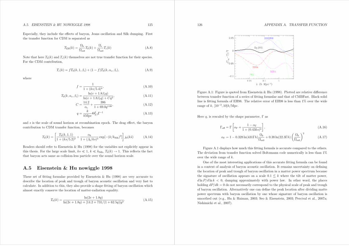
A.5. EISENSTEIN & HU NOWIGGLE 1998 125
Especially, they include the effects of baryon, Jeans oscillation and Silk dumping. First
the transfer function for CDM is separated as
TEH(k) =ΩbΩm0
Tb(k) +ΩcΩm0
Tc(k) (A.8)
Note that here Tb(k) and Tc(k) themselves are not true transfer function for their species.
For the CDM contribution,
Tc(k) = fT0(k, 1, βc) + (1− f)T0(k, αc, βc), (A.9)
where
f =1
1 + (ks/5.4)4, (A.10)
T0(k, αc, βc) =ln(e+ 1.8βcq)
ln(e+ 1.8βcq) + Cq2, (A.11)
C =14.2
αc+
386
1 + 69.0q1.08, (A.12)
q =k
hMpcΘ22.7Γ
−1 (A.13)
and s is the scale of sound horizon at recombination epoch. The drag effect, the baryon
contribution to CDM transfer function, becomes
Tb(k) =
[T0(k, 1, 1)
1 + (ks/5.2)2+
αb1 + (βb/ks)3
exp[−(k/kSilk)4]]j0(ks) (A.14)
Readers should refer to Eisenstein & Hu (1998) for the variables not explicitly appear in
this thesis. For the large scale limit, ks 1, k kSilk, Tb(k)→ 1. This reflects the fact
that baryon acts same as collision-less particle over the sound horizon scale.
A.5 Eisenstein & Hu nowiggle 1998
These set of fitting formulae provided by Eisenstein & Hu (1998) are very accurate to
describe the location of peak and trough of baryon acoustic oscillation and very fast to
calculate. In addition to this, they also provide a shape fitting of baryon oscillation which
almost exactly conserve the location of matter-radiation equality.
T0(k) =ln(2e+ 1.8q)
ln(2e+ 1.8q) + [14.2 + 731/(1 + 62.5q)]q2. (A.15)
126 APPENDIX A. TRANSFER FUNCTION
Figure A.1: Figure is quoted from Eisenstein & Hu (1998). Plotted are relative difference
between transfer function of a series of fitting formulae and that of CMBFast. Black solid
line is fitting formula of EH98. The relative error of EH98 is less than 1% over the wide
range of k, [10−3, 10]h/Mpc.
Here q, is rescaled by the shape parameter, Γ as
Γeff = Γ
[αΓ +
1− αΓ1 + (0.43ks)4
], (A.16)
αΓ = 1− 0.328 ln(431Γh) Ωb
Ωm0
+ 0.38 ln(22.3Γh)
(Ωb
Ωm0
)2
(A.17)
Figure A.1 displays how much this fitting formula is accurate compared to the others.
The deviation from transfer function solved Boltzmann code numerically is less than 1%
over the wide range of k.
One of the most interesting applications of this accurate fitting formula can be found
in a context of analysis of baryon acoustic oscillation. It remains uncertainty on defining
the location of peak and trough of baryon oscillation in a matter power spectrum because
the signature of oscillation appears on a scale 0.1 k where the tilt of matter power,
d lnP/d ln k < 0, damping approximately with power law. In other word, the places
holding dP/dk = 0 do not necessarily correspond to the physical scale of peak and trough
of baryon oscillation. Alternatively one can define the peak location after dividing matte
power spectrum with baryon oscillation by one whose signature of baryon oscillation is
smoothed out (e.g., Hu & Haiman, 2003; Seo & Eisenstein, 2003; Percival et al., 2007a;
Nishimichi et al., 2007).
A.6. EFFECT OF NEUTRINO 127
A.6 Effect of Neutrino
Hu & Eisenstein (1998); Eisenstein & Hu (1999) encode the spacially dependent suppres-
sion due to the neutrino free streaming into the growth rate. So in this case the growth rate
depends both on time and scale. In such a situation, total matter is sum of CDM, baryon
and (massive) neutrino; Ωm = Ωc+Ωb+Ων , alternatively, 1 = fcb+ fν = fc+ fb+ fν with
fi = Ωi0/Ωm0. Focused on the specific species, the transfer function of CDM + baryon
(+ neutrino) can be decomposed into
Tcb(q, z) = Tmaster(q)Dcb(q, z)
D1(z), (A.18)
Tcbν(q, z) = Tmaster(q)Dcbν(q, z)
D1(z), (A.19)
where the wave number q is given at equation (A.13), D1 is growth factor without neutrino
free streaming normalized to unity at equality time, which evolves with time proportional
to a in a matter dominated universe. If dark energy is cosmological constant, D1 can be
expressed in an integral form (e.g., Heath, 1977), or given by useful fitting formula (Lahav
et al., 1991; Carroll et al., 1992) otherwise can be solved numerically (e.g., Matsubara &
Szalay, 2003). The scale dependencies after recombination are encapsulated into Dcb(q, z)
and Dcbν(q, z). Tmaster(q) is time independent universal transfer function; the physics of
scale dependency only before the recombination epoch is incorporated. With the neu-
trino free streaming, growth of density after recombination is logarithmic below the free
streaming scale(Bond et al., 1980) according to the factor,(Hu & Eisenstein, 1998)
pi := (5−√1 + 24fi)/4 (A.20)
where i = cb, c. Then the growth factors in the presence of free streaming are
Dcb(q, z) =
[1 +D1(z)
1 + yfs(q, fν)
]pcb/0.7
D1(z)1−pcb , (A.21)
Dcbν(q, z) =
f0.7/pcb
cb +
[1 +D1(z)
1 + yfs(q, fν)
]pcb/0.7
D1(z)1−pcb . (A.22)
Here, y is free streaming epoch as a function of scale,
yfs(q, fν) = 17.2fν(1 + 0.488f−7/6ν )(Nνq/fν)
2, (A.23)
where Nν is number of flavors of massive neutrino. In the absence of massive neutrinos,
master function Tmaster is exactly same as CDM + baryon case(equation (A.8)). This
agreement can be seen even in the presence of some species of neutrinos on the scale
128 APPENDIX A. TRANSFER FUNCTION
larger than sound horizon at recombination epoch and than horizon at the epoch when the
significant neutrino become non-relativistic. Hu & Eisenstein (1998) solves the evolution
equations analytically in the small scale limit, and estimate the amount of suppression on
small scale.
αν(fν , fb, yd) =fcfcb
5− 2(pc + pcb)
5− 4pcb (A.24)
× 1− 0.553fνb + 0.126f 3νb1− 0.193√fνNν + 0.169fνN0.2
ν
(1 + yd)pcb−pc
×1 +
pc − pcb2
[1 +
1
(3− 4pc)(7− 4pcb)](1 + yd)
−1
The fitting formula is developed keeping these two limit solutions in mind (Eisenstein &
Hu, 1999). As an analogy of the case of no-wiggle fitting formula, they rescale the shape
parameter as
Γeff = Γ
[√αν +
1−√αν1 + (0.43ks)4
], (A.25)
qeff =Θ22.7Γeff
k
hMpc−1(A.26)
Using this rescaled wave number allows to fit the effective amount of suppression due to
the baryon and neutrino.
Tsup(k) =ln(e+ 1.84βc
√ανqeff)
ln(e+ 1.84βc√ανqeff) + [14.4 + 325/(60.5q1.11eff )]q2eff
(A.27)
where βc = (1 − 0.949fνb)−1. Although this fitting well represents a behavior of trans-
fer function suppressed by baryon and neutrino before the recombination, overestimate
should be occurred due to the incomplete treatment on the transition scale where neutrino
becomes gradually non-relativistic. For the baryon fraction, fb 0.3, this overshoot can
be compensated by the following correction term,
B(k) = 1 +1.2f 0.64ν N0.3+0.6fν
ν
q−1.6ν + q0.8ν, (A.28)
qν = 3.92√Nνq/fν (A.29)
Then the master function is
Tmaster(k) = Tsup(k)B(k). (A.30)
Standard model of element particle predicts the number of generations of neutrino is
three. The measurement of cross section of Z boson reveals that the number of flavors of
A.6. EFFECT OF NEUTRINO 129
light neutrino well agrees with 3 (e.g., Brandt et al., 2000). Recently the solar, atmospheric
man-made and long-baseline neutrino observations such as SuperKamiokande detect the
strong signal of neutrino oscillation, which can be direct consequence of the existence of
mass in neutrino by measuring the delta mass squared(Ahn et al., 2006) in a two flavor
oscillation scenario. This result well agrees with the number of flavors of neutrino. On
the contrary, LSND group (Athanassopoulos et al., 1995; Hill, 1995) report the extra
channel of neutrino oscillation,νµ → νe, which suggests the existence of 4th flavor of
neutrino, sterile neutrino. Okada & Yasuda (1997) gives a review of the constraint on
sterile neutrino from experiments of neutrino oscillation and the impacts on cosmology.
Viel et al. (2005) investigates the effect of sterile neutrino as a candidate of warm dark
matter on the matter power spectrum and give some constraints on mass of sterile neutrino
through the Ly-α forest.
130 APPENDIX A. TRANSFER FUNCTION
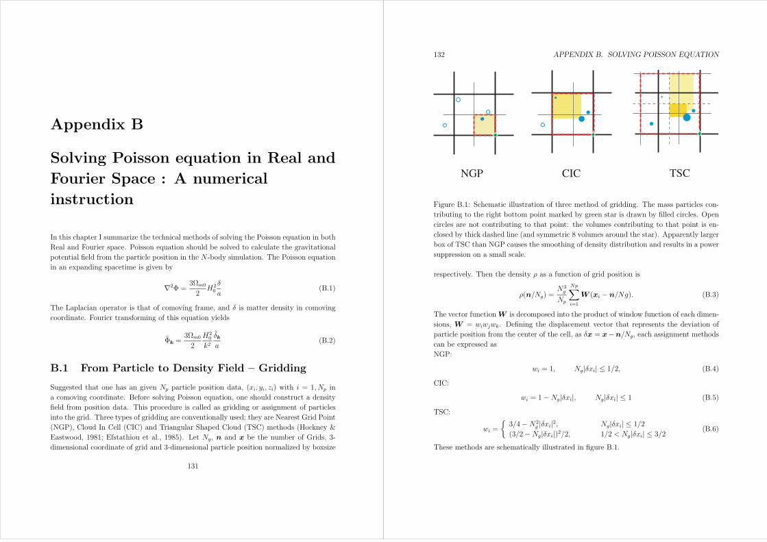
Appendix B
Solving Poisson equation in Real and
Fourier Space : A numerical
instruction
In this chapter I summarize the technical methods of solving the Poisson equation in both
Real and Fourier space. Poisson equation should be solved to calculate the gravitational
potential field from the particle position in the N -body simulation. The Poisson equation
in an expanding spacetime is given by
∇2Φ =3Ωm0
2H20
δ
a(B.1)
The Laplacian operator is that of comoving frame, and δ is matter density in comoving
coordinate. Fourier transforming of this equation yields
Φk =3Ωm0
2
H20
k2δk
a(B.2)
B.1 From Particle to Density Field – Gridding
Suggested that one has an given Np particle position data, (xi, yi, zi) with i = 1, Np in
a comoving coordinate. Before solving Poisson equation, one should construct a density
field from position data. This procedure is called as gridding or assignment of particles
into the grid. Three types of gridding are conventionally used; they are Nearest Grid Point
(NGP), Cloud In Cell (CIC) and Triangular Shaped Cloud (TSC) methods (Hockney &
Eastwood, 1981; Efstathiou et al., 1985). Let Ng, n and x be the number of Grids, 3-
dimensional coordinate of grid and 3-dimensional particle position normalized by boxsize
131
132 APPENDIX B. SOLVING POISSON EQUATION
NGP CIC TSC
Figure B.1: Schematic illustration of three method of gridding. The mass particles con-
tributing to the right bottom point marked by green star is drawn by filled circles. Open
circles are not contributing to that point: the volumes contributing to that point is en-
closed by thick dashed line (and symmetric 8 volumes around the star). Apparently larger
box of TSC than NGP causes the smoothing of density distribution and results in a power
suppression on a small scale.
respectively. Then the density ρ as a function of grid position is
ρ(n/Ng) =N3g
Np
Np∑i=1
W (xi − n/Ng). (B.3)
The vector function W is decomposed into the product of window function of each dimen-
sions, W = wiwjwk. Defining the displacement vector that represents the deviation of
particle position from the center of the cell, as δx = x−n/Ng, each assignment methods
can be expressed as
NGP:
wi = 1, Ng|δxi| ≤ 1/2, (B.4)
CIC:
wi = 1−Ng|δxi|, Ng|δxi| ≤ 1 (B.5)
TSC:
wi =
3/4−N2
g |δxi|2, Ng|δxi| ≤ 1/2
(3/2−Ng|δxi|)2/2, 1/2 < Ng|δxi| ≤ 3/2(B.6)
These methods are schematically illustrated in figure B.1.
B.2. DIFFERENCE SCHEME 133
B.2 Difference Scheme
It is straightforward to calculate gravitational potential field in a real space once obtaining
the density field by means of above gridding methods. In the real space, the differential
equation can be solved numerically by Successive Over Relaxation(SOR) method well
known as the Gauss-Seidel’s method or Jacobi’s method for the special case. Let me
rewrite the Poisson equation as ∇2Φi,j,k = κδijk where κ = 3Ωm0H20/2a and i, j, k denote
the 3D-coordinate in the grid. Replacing the Laplacian by Central Difference yields
Φi,j,k =1
6(Φi−1,j,k + Φi+1,j,k + Φi,j−1,k + Φi,j+1,k + Φi,j,k−1 + Φi,j,k+1 − κδi,j,k) (B.7)
In principle, iterating this infinitely yields a convergence to the collect answer of Φi,j,k.
In practice, the sufficient large number of iteration can achieve a solution with a desired
accuracy. Denoting Φni,j,k the solution after the nth iteration, equation (B.7) can be
rewritten with preferred weight C(1 ≤ C ≤ 2) as
Φn+1i,j,k = Φn
i,j,k + C
[1
6(Φn
i−1,j,k + Φni+1,j,k+
Φni,j−1,k + Φ
ni,j+1,k + Φ
ni,j,k−1 + Φ
ni,j,k+1 − κδi,j,k)− Φn
i,j,k
]. (B.8)
The boundary condition is set to periodic which is consistent with that of Fourier space
solvent. C = 1.7 enables us to converge twice faster than the case of C = 1, which
corresponds to Gauss-Seidel’s method and gives a best performance for this calculation.
B.3 FFT Scheme
Although the SOR method with its weight being most efficient one gives faster convergence
for solving Poisson equation, it costs enormous calculation time compared to FFT scheme.
As seen in equation (B.2), Fourier transform reduce the differential equation into easier
form. All one should do is Fourier transforming the density field and multiplying κ/k2, and
then inverse Fourier transforming. Efficient way of this procedure is given by Efstathiou
et al. (1985) as
Φi,j,k = κ∑p,q,r
Gp,q,rδp,q,r exp[2πi(ip+ jq + kr)/Ng] (B.9)
where the Green function of Laplacian is given by seven point Finite-Difference Approxi-
mation(FDA)
Gp,q,r =
0, i = j = k = 0,
−π/Ng
[sin2(πp/Ng) + sin
2(πq/Ng) + sin2(πr/Ng)
], otherwise
(B.10)
134 APPENDIX B. SOLVING POISSON EQUATION
I found both real and Fourier space solvents agree very well though real space method
takes 30 minutes for Ng = 643 while Fourier space method takes 10 seconds for same
number of grid. This might scales as ∼ N/ log(N).
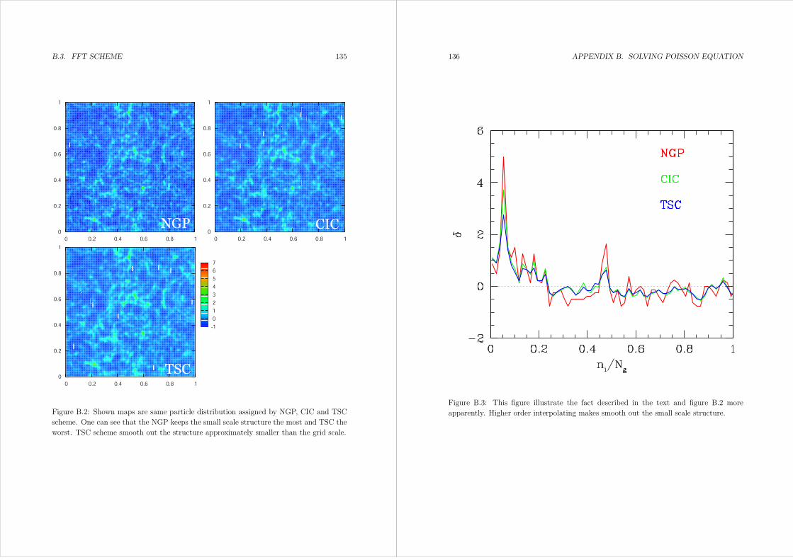
B.3. FFT SCHEME 135
0 0.2 0.4 0.6 0.8 1
0
0.2
0.4
0.6
0.8
1
0 0.2 0.4 0.6 0.8 1
0
0.2
0.4
0.6
0.8
1
-1
0
1
2
3
4
5
6
7
0 0.2 0.4 0.6 0.8 1
0
0.2
0.4
0.6
0.8
1
NGP CIC
TSC
Figure B.2: Shown maps are same particle distribution assigned by NGP, CIC and TSC
scheme. One can see that the NGP keeps the small scale structure the most and TSC the
worst. TSC scheme smooth out the structure approximately smaller than the grid scale.
136 APPENDIX B. SOLVING POISSON EQUATION
Figure B.3: This figure illustrate the fact described in the text and figure B.2 more
apparently. Higher order interpolating makes smooth out the small scale structure.

Appendix C
Derivation of integrated Sachs Wolfe
effect
In this appendix, I derive the Integrated Sachs Wolfe (Rees Sciama) effect mainly based
on (Sachs & Wolfe, 1967) in the conformal Newtonian gauge representation.
To begin with, consider the decomposition of metric perturbation into scalar, vector
and tensor mode. The vector quantity h0i ≡ Bi can be divided into the contribution from
scalar and others. The tensor quantity hij ≡ Cij can be divided into the contribution
from scalar, vector and the part proportional to the background spacial metric,
h00 ≡ −2a2A (C.1)
h0i ≡ −a2Bi = −a2(B(s)|i +B
(v)i ) (C.2)
hij ≡ 2a2Cij = 2a2(Dγij + C(s)|ij +
1
2[C
(v)i|j + C
(v)j|i ] + C
(T )ij ). (C.3)
Note that subscript | denotes the 3 dimensional covariant derivative, i.e.Xi|j = Xi,j +
(3)ΓkijXk, (C.4)
(3)Γijk =1
2γia(γja,k + γka,j − γjk,a)). (C.5)
Now one should remind the condition that the scalar quantity can not be generated from
the vector mode and that the vector and scalar quantity can not be generated from the
tensor mode,
B(v)|ii = 0, (C.6)
C(v)|ii = 0, C
(T )ii = 0, C
(T )|iij = 0. (C.7)
Since the Newtonian(longitudinal) gauge fixes variables as B(s) = C(s) = 0, the gauge in-
variant variables are Φ = A,Ψ = D. Here suppose that only the scalar mode is considered
137
138 APPENDIX C. DERIVATION OF ISW
and ignoring the anisotropic stress, Φ = −Ψ, then the metric becomes
ds2 = a2[(1 + 2Φ)dτ − (1− 2Φ)γijdxidxj]. (C.8)
Denoting the wave-vector which is tangential to the photon geodesic as
kµ :=∂xµ
∂w, (C.9)
the non perturbed geodesic equation becomes
− d2 0τ
dw2=1
2γ′ij 0k
i0k
j = 0 (C.10)
− d2 0xi
dw2= (3)Γijl 0k
j0k
l = 0. (C.11)
The solutions of this equation are
0τ = τ0 − w (C.12)
0xi = eiw, (C.13)
where w is affine parameter, and ei is a unit vector pointing to the ki. The subscript
0 in the left bottom of variable denotes the unperturbed quantity and 1 is first order
perturbation quantity. The first-order of geodesic equations are
d
dw
(d 1τ
dw− 2Φ
)=
∂Φ
∂τ(1 + γij 0k
i0k
j) (C.14)
d
dwγij
(2Φ 0k
j − 0kj)= Φ,i + (Φγjl),i + 0k
j0k
l. (C.15)
Integrating yields
d 1τ
dw= 1k
0 = 2
[Φ +
∫ w
0
∂Φ
∂τdw′
], (C.16)
d 1xi
dw= 1k
i = 2
[Φei −
∫ w
0
∂Φ
∂τdxi
]. (C.17)
Next, we will see how the four velocity can be expressed up to the first order. The uniform
component is
0uµ = a(1, 0, 0, 0), 0uµ = 0. (C.18)
The sum of zero-th and first order yields
uµ = a(1 +X, vi), (C.19)
139
where I put vi = ui/u0 is 3D velocity. Note that the inner product in any coordinate
system must be unity, uµuµ = 1. Thus we have
uµ = a(1− Φ, vi), (C.20)
uµ = a−1(−1− Φ, vi). (C.21)
Recalling that the redshift is defined as the ratio of photon energy at emitter and receiver
projected to the fluid, and keeping in mind that we are moving with the cosmological
fluid, then
z + 1 =(kµuµ)w=τ0−τ∗(kνuν)w=0
, (C.22)
where asterisk ∗ denotes the epoch of decoupling. Substituting equation (C.20) into
equation (C.22) yields
z + 1 =a0a∗
[1 + Φ(τ0)− Φ(τ∗) + 2
∫ τ0−τ∗
0
∂Φ
∂τdw
]. (C.23)
As the temperature of CMB redshifts as
T0 =1
1 + zT∗ = T∗
a∗a0
(1 +
∆T
T
)(C.24)
Thus the temperature anisotropy becomes
∆T
T= −Φ(τ0) + Φ(τ∗)− 2
∫ τ0−τ∗
0
∂Φ
∂τdτ. (C.25)
The first term is the monopole which we can in principle not observe and second term
represent the temperature anisotropy caused by the gravitational redshift due to the
potential fluctuations at last scattering surface, the Sachs Wolfe effect. The integral
term represent the temperature anisotropy caused by the time variation of gravitational
potential integrated along the line of sight, the integrated Sachs Wolfe effect.