˘ ˇˆ ˙˝ ˛ ˙ˇ - ireservoir.com - your e-solution for global energy€¦ · ·...

R e s e r v o i r c h a r a c t e r i z at i o n

62 The Leading Edge January 2011

SPECIAL SECTION: R e s e r v o i r c h a r a c t e r i z at i o n

��

Crossplots are commonly used in the geosciences to gain qualitative insight about relationships between different

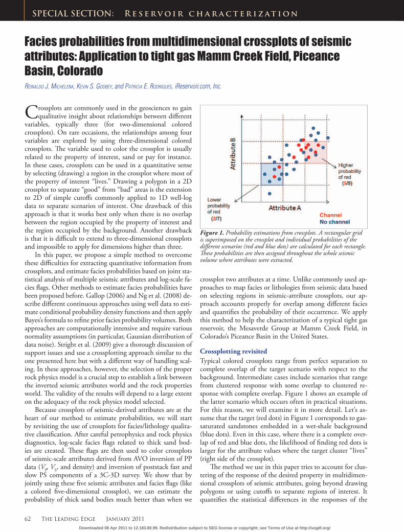
variables, typically three (for two-dimensional colored crossplots). On rare occasions, the relationships among four variables are explored by using three-dimensional colored crossplots. The variable used to color the crossplot is usually related to the property of interest, sand or pay for instance. In these cases, crossplots can be used in a quantitative sense by selecting (drawing) a region in the crossplot where most of the property of interest “lives.” Drawing a polygon in a 2D crossplot to separate “good” from “bad” areas is the extension to 2D of simple cutoffs commonly applied to 1D well-log data to separate scenarios of interest. One drawback of this approach is that it works best only when there is no overlap between the region occupied by the property of interest and the region occupied by the background. Another drawback is that it is difficult to extend to three-dimensional crossplots and impossible to apply for dimensions higher than three.

In this paper, we propose a simple method to overcome these difficulties for extracting quantitative information from crossplots, and estimate facies probabilities based on joint sta-tistical analysis of multiple seismic attributes and log-scale fa-cies flags. Other methods to estimate facies probabilities have been proposed before. Gallop (2006) and Ng et al. (2008) de-scribe different continuous approaches using well data to esti-mate conditional probability density functions and then apply Bayes’s formula to refine prior facies probability volumes. Both approaches are computationally intensive and require various normality assumptions (in particular, Gaussian distribution of data noise). Stright et al. (2009) give a thorough discussion of support issues and use a crossplotting approach similar to the one presented here but with a different way of handling scal-ing. In these approaches, however, the selection of the proper rock physics model is a crucial step to establish a link between the inverted seismic attributes world and the rock properties world. The validity of the results will depend to a large extent on the adequacy of the rock physics model selected.

Because crossplots of seismic-derived attributes are at the heart of our method to estimate probabilities, we will start by revisiting the use of crossplots for facies/lithology qualita-tive classification. After careful petrophysics and rock physics diagnostics, log-scale facies flags related to thick sand bod-ies are created. These flags are then used to color crossplots of seismic-scale attributes derived from AVO inversion of PP data (VP, VS, and density) and inversion of poststack fast and slow PS components of a 3C-3D survey. We show that by jointly using these five seismic attributes and facies flags (like a colored five-dimensional crossplot), we can estimate the probability of thick sand bodies much better than when we

REINALDO J. MICHELENA, KEVIN S. GODBEY, and PATRICIA E. RODRIGUES, iReservoir.com, Inc.

crossplot two attributes at a time. Unlike commonly used ap-proaches to map facies or lithologies from seismic data based on selecting regions in seismic-attribute crossplots, our ap-proach accounts properly for overlap among different facies and quantifies the probability of their occurrence. We apply this method to help the characterization of a typical tight gas reservoir, the Mesaverde Group at Mamm Creek Field, in Colorado’s Piceance Basin in the United States.

Crossplotting revisitedTypical colored crossplots range from perfect separation to complete overlap of the target scenario with respect to the background. Intermediate cases include scenarios that range from clustered response with some overlap to clustered re-sponse with complete overlap. Figure 1 shows an example of the latter scenario which occurs often in practical situations. For this reason, we will examine it in more detail. Let’s as-sume that the target (red dots) in Figure 1 corresponds to gas-saturated sandstones embedded in a wet-shale background (blue dots). Even in this case, where there is a complete over-lap of red and blue dots, the likelihood of finding red dots is larger for the attribute values where the target cluster “lives” (right side of the crossplot).

The method we use in this paper tries to account for clus-tering of the response of the desired property in multidimen-sional crossplots of seismic attributes, going beyond drawing polygons or using cutoffs to separate regions of interest. It quantifies the statistical differences in the responses of the

Figure 1. Probability estimations from crossplots. A rectangular grid is superimposed on the crossplot and individual probabilities of the different scenarios (red and blue dots) are calculated for each rectangle. These probabilities are then assigned throughout the whole seismic volume where attributes were extracted.

Downloaded 08 Apr 2011 to 12.183.80.99. Redistribution subject to SEG license or copyright; see Terms of Use at http://segdl.org/

January 2011 The Leading Edge 63


different scenarios. As we will show in the next section, our approach is completely data-driven, because it doesn’t require any model to relate the property of interest with the seismic attributes. The next section shows the details of the method starting from basic probability definitions.

Probabilities from crossplotsWe use conditional probabilities and the correspondence of the different log-scale scenarios with seismic-scale attributes sampled at well locations to estimate the likelihood of the target scenario away from wells. Similar results can be ob-tained using Bayes’s formula to estimate the probability if a prior estimate of probability is known.

A conditional probability estimates the likelihood of an event of interest given that a conditioning event is known to occur:

Here, P(S) is the probability of observing the target sce-nario S (e.g., facies flag related to thick sand bodies), and A is a conditioning event providing extra information (in our case, inverted seismic attributes).

Conditional probabilities are well suited to this applica-tion because they do not require that any particular form of relationship, or even any relationship at all, exists between scenarios (facies) and conditioning events (seismic attributes). Additionally, no assumptions are made about probability dis-tributions or independence.

For the case of two attributes shown in Figure 1, we define conditioning events by superimposing an M × N grid on the attribute crossplot; each rectangular cell in the grid defines a conditioning event. These events should capture any rela-tionship between facies and seismic attributes. This approach easily generalizes to cases where more than two attributes are believed to be related to the target scenario. Examples of us-ing two, three, and five attributes at a time are shown later in this paper.

Selection of M and N for defining conditioning events in-volves a tradeoff and should be done on a case-by-case basis. Large M and N (small rectangles) will tend to group closely related samples and give stronger separation, but grid cells that are too small could mean sensitivity to noise and other errors. On the other hand, small M and N (large rectangles) will group more loosely related samples and give weaker sepa-ration, but larger grid cells mean more stable, but lower-reso-lution, estimates.

As shown in Figure 1, the probability is the ratio of the number of points in a grid cell related to the target scenario over the total number of points in the same cell. In this sense, we can interpret the probabilities as a seismic-scale estimate of net-to-gross for a given set of attribute ranges. The total number of points per cell provides an estimate of the reliabil-ity of the probabilities and can be used to assign confidence estimates to the interpretation of the probability results.

The next section shows an example of the application of this method.

Field data example: Mamm Creek FieldMamm Creek Field is in the Piceance Basin of northwestern Colorado in the United States. Most of the gas production in Mamm Creek comes from fluvial tight sands (~5000 ft deep) in the Williams Fork Formation, but marine sands in the Corcoran, Cozzette, and Rollins members (~7000 ft deep) of the Iles Formation and the middle and upper sands of the Williams Fork Formation also contribute to production (Scheevel and Cumella, 2009). Mapping the distribution of sands is critical for early effective development of the field but, unfortunately, seismic data have not been used exten-sively for this purpose because elastic properties of sands and shales show large overlap in rock physics diagnostics. Estima-tion of sand distribution in the upper fluvial tight sands is much more challenging than in the lower marine sands be-cause fluvial sands are thinner and more discontinuous than thicker, regionally continuous marine sands. The method presented in this paper was applied separately to both fluvial and marine intervals.

The data set used for this study consisted of log data from 102 wells, a 3D prestack compressional seismic data set and two PS (fast and slow) stacked volumes from a 3D converted-wave multicomponent data set. The PS data set was not ac-quired at the same time as the 3D compressional data. Gam-ma-ray, neutron, and density logs are available in most wells. Sonic data were available at three wells only; one well had a dipole sonic and another well had an oriented cross-dipole sonic. Figure 2 shows the well locations within the study area of 2.5 square miles.

A summary of our workflow follows:

1) Petrophysical analysis and generation of facies flags based on lithology and thickness. Only sand intervals with more than 6% effective porosity and thickness greater than 10–15 ft were kept for seismic calibration. This approach acknowledges the difficulty of detecting sand bodies of less than 10 ft with seismic data and, therefore, no attempt is made to map them.

2) Log-scale analysis of relationships between petrophysical properties of target facies and seismic attributes derived from AVO inversion and inversion of PS stacked data. VP, VS, density, and shear impedances derived from PS data were the key attributes in this analysis. Crossplots of these different attributes derived from log data are shown in Fig-ure 3. These crossplots at log scale are used only to make sure similar crossplots at seismic scale show the expected qualitative behaviors.

3) Horizon interpretation from PP and PS data. PS fast and slow volumes were interpreted for the same horizons as the ones interpreted in the 3D compressional-wave data. Con-sistency between the interpretations of PP and PS data was achieved by looking at not only the character of the seis-mic events but also the well ties in PP and PS time using density, sonic, and shear logs.

4) Three-term AVO inversion of PP prestack gathers and poststack inversion of 3D PS stacked data. The results of this step are volumes of VP, VS, density (rho), pseudo




S-impedance fast (pSIf ) and pseudo S-impedance slow (pSIs). Pseudo S-impedances from PS stacked data were estimated using the algorithm described in Guliyev and Michelena (2009). Since the study area is small, only one well was used to build the background model in each of these in-versions. Due to the lack of measured compressional and shear logs in most wells, seismic well ties and quality control of inverted acoustic imped-ance, shear impedance, and pseudo S-impedances relied on synthetic P and S logs generated from existing density, gamma-ray, and neutron logs using artificial neural networks. These syn-thetic logs were considered adequate for these purposes and were not used for any other quantitative analysis. Re-liability of density inversion, however,

Figure 2. Well locations within the study area of 2.5 square miles in sections 20, 21, and 28 of Mamm Creek Field. Bottom-hole locations are indicated by yellow circles and well trajectories are shown in blue.

Figure 3. Crossplots of log-scale attributes at one well location color-coded by facies flags at log scale. Sand response is clearly clustered in all crossplots but elastic properties of sands show a total overlap with the properties of the background rocks (mostly shales). Red arrows indicate the area of the crossplot where the sands tend to cluster with respect to the background. Departures from the 45˚ line in the lower right crossplot of impedances from PS fast versus PS slow (pSI fast and pSI slow, respectively) data indicate azimuthal anisotropy. Thick sand facies tend to be more anisotropic than the sourrouding shales, in particular in the marine interval. These crossplots give a clear idea of what to expect when crossplotting the same attributes estimated from seismic data.




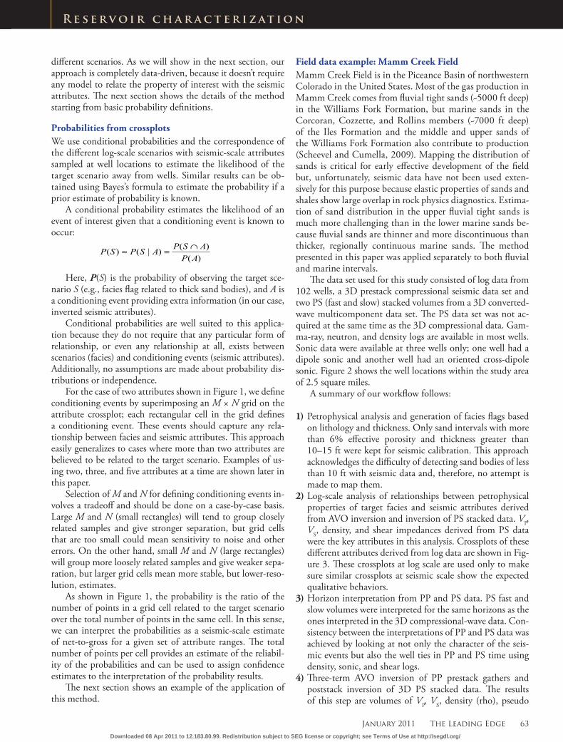
Figure 4. Crossplots of seismic-scale inverted attributes at 30 well locations color-coded by facies flags at log scale. The overall position in the crossplot of thick sands (red) with respect to the background (cyan) is as expected from rock physics diagnostics at log scale (Figure 3). Departures from the 45˚ line in crossplot (d) of impedances from PS fast versus PS slow data indicate azimuthal anisotropy. As expected in this field from Figure 3, thick sand facies tend to be more anisotropic.

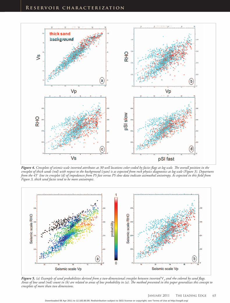
Figure 5. (a) Example of sand probabilities derived from a two-dimensional crossplot between inverted VP and rho colored by sand flags. Areas of low sand (red) count in (b) are related to areas of low probability in (a). The method presented in this paper generalizes this concept to crossplots of more than two dimensions.




Figure 6. Log data versus probability estimates from seismic data using different combinations of attributes at well 21B-28 within the marine interval. (a) Gamma ray; (b) sand flag; (c) moving average of sand flag; (d) to (h) probabilities from seismic attributes. (d) VP-VS; (e) VP-rho; (f ) VS-rho; (g) VP-VS-rho; (h) VP-V,-rho-pSIf-pSIs. Only 30 wells (out of 102) were used to train the seismic data in this example.

Figure 7. Thick sand probability from seismic data extracted along a cross section of 102 wells from a 3D probability cube for the marine interval of Mamm Creek Field. These probabilities were estimated by using five inverted seismic attributes and thick-sand flags shown in Figure 8. (Red = higher probability and green = lower probability). Since the separation between wells is not constant, we do not show a horizontal scale in this cross section. The smallest separation between neighboring wells in the field, however, can be up to 330 ft (see Figure 2).

Figure 8. Log-scale thick sand facies flags along a cross section of 102 wells overlain on seismic probabilities shown in Figure 7. Since the separation between wells is not constant, we do not show a horizontal scale in this cross section. The smallest separation between neighboring wells in the field, however, can be up to 330 ft (see Figure 2).

was confirmed by density logs available in almost all well locations.

5) Velocity model building and time-to-depth conversion of seismic-derived information honoring depths of five formation tops picked along 102 wells. Three separate ve-locity models were built to perform depth conversion of compressional, fast PS, and slow PS volumes, respectively.

6) Extraction of seismic-derived attributes along well trajec-tories in depth using a sampling interval of 1 ft. This ap-parent “oversampling” of the seismic data along the well trajectories will help to compare, in a statistical sense, the seismic-scale response with the log-scale facies flags.

7) Crossplots of seismic-derived attributes colored by log-scale facies within intervals of similar geologic character-istics, either fluvial or marine. Figure 4 shows examples of these crossplots for the marine section of Mamm Creek Field. Even though seismic-scale crossplots in Figure 4 show more scatter than log-scale crossplots in Figure 3 (due to scale differences of the measurements, inaccuracies in inversion results and well-seismic mis-ties due to poor velocity control in areas away from well markers), red sand flags in Figure 4 tend to fall in the same crossplot areas predicted by log-scale analysis (see Figure 3). Although not shown here, thick sands tend to cluster much more than thin sands in seismic-scale crossplots. This makes sense if




Figure 9. Comparison of log-scale information (gamma-ray, sand flag, thick-sand flag, average sand flag), seismic-scale information (inverted VP, VS, and rho above bracket), and sand probability curve. The joint use of log- and seismic-scale information in the probabilistic sense explained in this paper yields a higher-resolution attribute than the individual inverted results (VP, VS, and rho) used as input.

we think that thick sand bodies are easier to “see” at seismic scale than thin bodies. Different crite-ria were used to create thickness-related sandy facies flags. We se-lected the one that produced a more clustered seismic response in 2D crossplots, usually related to sand thickness of about 10-15 ft.

8) Estimation of probabilities of thick sand bodies using different combinations of inverted seis-mic attributes. Figure 5a shows an example of probabilities esti-mated using the two-dimensional crossplot between inverted VP and inverted rho shown in Figure 5b. Areas with a low count of sand flags yield lower probabilities than areas with higher count of flags. Among the attribute com-binations (crossplots) tested, the most relevant were VP-VS, VP-rho, VS-rho, VP-VS-rho, and VP-VS-rho-pSIf-pSIs. Figure 6 shows the results of probabilities estimated from different attribute combina-




tions at a selected well location. The poorest predictions are obtained when using a VP-VS crossplot alone (Figure 6d). Predictions are considerably improved when including density in the analyses (Figures 6e and 6f ). The best predictions, when using P-wave data attributes only, are obtained by combining VP, VS, and rho (Figure 6g). Finally, when P-wave and mul-ticomponent-derived attributes are used si-multaneously in the form of a five-dimensional crossplot, we obtain the best predictions (Figure 6h); estimated prob-abilities resemble very closely the average of the facies flags from well data (Figure 6c). As shown in Figure 4d, PS at-tributes are sensitive to sand anisotropy and for this reason including these attributes in the analysis helps to improve the detection of thick sand facies in the marine portion of the field. As explained in the section “Probabilities from crossplots”, the number of classes used to grid the attribute crossplots (M x N in a 2D crossplot) was determined after examining the results of different numbers and looking for a compromise between resolution and stability. We con-sidered 50 classes per attribute adequate for this particular data set.

Notice that even though none of the crossplots in Figure 4 shows separation between thick sands and background fa-cies, the joint probabilistic analysis of all attribute responses still yields good estimates of probabilities of thick sand facies.

Out of the 102 wells available for this study (see Figure 2), we started testing the probability estimations by using only 30 wells selected from the original 102 wells with the only crite-rion that they covered the study area evenly. Figure 6 shows an example of the result of training the seismic data with 30 wells only. Blind tests (not shown) were also conducted to test the predictive power of probability estimations in wells not used to train the seismic data. Probabilities were also computed by training the seismic data extracted along all 102 wells with fa-cies flags generated along the same wells. The purpose of this test was to understand how much predictions could be im-proved by introducing all well data available. Figure 7 shows a cross section of the five-seismic-attribute-derived probabilities along the 102 wells. A cross section of facies flags used to color the five-dimensional crossplot is shown in Figure 8 overlain on the seismic-derived probabilities. Notice how facies dis-tribution expected from log data agrees well with estimated probabilities from seismic. The fact that the result is not per-fect means that sand flags used to train the seismic data do not act as hard constraints in the final probability estimations.

Figure 9 shows an example of the results in the fluvial in-terval at a selected well location. As expected, the joint use of log-scale and seismic-scale information in a probabilistic sense yields an attribute (the sand probability) with higher resolution than the original inversion results. The probabil-ity results, however, do not reproduce the log-scale average sand flag as closely as in the marine interval. This is expected because, as indicated earlier, mapping of fluvial sands in this field is a tougher problem than mapping of marine sands since the former are thinner and less continuous.

In addition to comparing directly the sand probabilities from seismic with sand flags along the wells to assess the quality of the results (Figures 6 to 9), we can do other types of comparisons. Figure 10 shows a comparison of a net-to-gross (NTG) sand map derived from interpolation of log data (Figure 10a) in an interval of 140 ft within the fluvial sec-tion with the average sand probabilities in the same interval (Figure 10b). Notice how the general trends are the same but seismic-derived probabilities contain additional details in the interwell region. Figure 10c shows a crossplot of NTG derived from well data versus average probabilities in the same interval where the maps were made. The correlation coefficient is very good (0.70) but the seismic tends to underestimate the NTG (the cloud of points in the crossplot is not centered around the diagonal). Besides lack of resolution of the seismic data to resolve all thin sands that are part of the net sand estimate from log data, another reason to explain this underestimation is that these thin sands were not used to train the seismic data.

ConclusionsFacies probabilities can be easily estimated from multidimen-sional crossplots of seismic attributes using basic probability definitions. The method yields useful results even when there is complete overlap of seismic attributes of target and back-ground facies, as long as the target facies show at least some clustering. No rock physics model is assumed to link the in-verted seismic attributes with the facies of interest which are identified at log scale using basic petrophysical principles. By analyzing log-scale and seismic-scale information in the same

Figure 10. (a) Net-to-gross (NTG) map created by interpolating net-sand values extracted from well data in an interval of 140 ft within the fluvial section. (b) Average sand probabilities from seismic data within the same interval. (c) Crossplot of NTG values and average probabilities extracted at the well locations. R2 is the correlation coefficient. Seismic-derived results show the same trends as well-derived maps but contain more detail in the interwell region. Compared to well-derived NTG, seismic-derived probabilities (NTG) tend to underestimate the sand content in this case. Information from 102 wells (red dots in the maps) was used to generate these figures (see Figure 2 for enlarged well locations).




framework (crossplots), probability results show higher reso-lution than original inverted seismic traces.

Application of this method at Mamm Creek Field shows that even when no single attribute or pair of attributes yields good separation of sand and background facies, probability estimates obtained by combining more than two attributes compare favorably with facies information at well locations. When using PP data only, good results are obtained by using simultaneously VP, VS, and density derived from three-term AVO inversion. However, the best results are obtained when using jointly these three attributes from PP data with fast and slow pseudo S-impedances derived from inversion of PS data. Sensitivity of PS amplitudes to azimuthal anisotropy helps to improve sand identification where sands are more anisotropic than the background.

Although not shown in this paper, the application of this approach yields seismic-scale estimates of facies-proportion curves that can be used to guide the construction of more detailed geological models (Michelena et al., 2009) using geo-statistical techniques. More research needs to be done to un-derstand how to use this methodology to help the calibration with log data of other seismic attributes such as structural or frequency-related.

ReferencesGallop, J., 2006, Facies probability from mixture distributions with

non-stationary impedance errors: 76th Annual International Meeting, SEG, Expanded Abstracts, 1801-1804.

Guliyev, E. and R. J. Michelena, 2009, Comparison of shear imped-ances inverted from stacked PS and SS data: Example from Ruli-son Field, Colorado: The Leading Edge, 28, no. 11, 1388–1393, doi:10.1190/1.3259618.

Michelena, R. J., K. S. Godbey, and O. Angola, 2009, Constraining 3D facies modeling by seismic-derived facies probabilities: Exam-ple from the tight-gas Jonah Field: The Leading Edge, 28, no. 12, 1470–1477, doi:10.1190/1.3272702.

Ng, S., P. Dahle, R. Hauge, and O. Kolbjørsen, 2008, Estimation of facies probabilities on the Snorre Field using geostatistical AVA inversion: 78th Annual International Meeting, SEG, Expanded Abstracts, 1971-1974.

Scheevel, J. and S. Cumella, 2009, Extracting sub-bandwidth detail from 3D amplitude data: An example from the Mesaverde Group, Piceance Basin, Colorado, U.S.A: The Leading Edge, 28, no. 11, 1362–1367, doi:10.1190/1.3259615.

Stright, L., A. Bernhardt, A. Boucher, T. Mukerji, and R. Derksen, 2009, Revisiting the use of seismic attributes as soft data for sub-seismic facies prediction: Proportions versus probabilities: The Leading Edge, 28, no. 12, 1460–1469, doi:10.1190/1.3272701.

Acknowledgments: The authors acknowledge Research Partnership to Secure Energy for America (RPSEA) for financial support, and the Bill Barrett Corporation (BBC) for providing much of the data that underlie this study. Steve Cumella, from BBC, provided valu-able geological insight about the field. Thanks to Mike Uland, from iReservoir, for many useful suggestions and comments.

Corresponding author: [email protected]


˘ ˇˆ ˙˝ ˛ ˙ˇ - ireservoir.com - your e-solution for global energy€¦ · ·...

Documents