1 finite element analysis methods - rice university finite element analysis methods 1.1 introduction...

Draft 12.0. Copyright 2009. All rights reserved. 7

1 Finite Element Analysis Methods

1.1 Introduction

The finite element method (FEM) rapidly grew as the most useful numerical analysis tool for engineers and applied mathematicians because of it natural benefits over prior approaches. The main advantages are that it can be applied to arbitrary shapes in any number of dimensions. The shape can be made of any number of materials. The material properties can be non‐homogeneous (depend on location) and/or anisotropic (depend on direction). The way that the shape is supported (also called fixtures or restraints) can be quite general, as can the applied sources (forces, pressures, heat flux, etc.). The FEM provides a standard process for converting governing energy principles or governing differential equations in to a system of matrix equations to be solved for an approximate solution. For linear problems such solutions can be very accurate and quickly obtained. Having obtained an approximate solution, the FEM provides additional standard procedures for follow up calculations (post‐processing), such as determining the integral of the solution, or its derivatives at various points in the shape. The post‐processing also yields impressive color displays, or graphs, of the solution and its related information. Today, a second post‐processing of the recovered derivatives can yield error estimates that show where the study needs improvement. Indeed, adaptive procedures allow automatic corrections and re‐solutions to reach a user specified level of accuracy. However, very accurate and pretty solutions of models that are based on errors or incorrect assumptions are still wrong.

When the FEM is applied to a specific field of analysis (like stress analysis, thermal analysis, or vibration analysis) it is often referred to as finite element analysis (FEA). FEA is the most common tool for stress and structural analysis. Various fields of study are often related. For example, distributions of non‐uniform temperatures induce non‐obvious loading conditions on solid structural members. Thus, it is common to conduct a thermal FEA to obtain temperature results that in turn become input data for a stress FEA. FEA can also receive input data from other tools like motion (kinetics) analysis systems and computation fluid dynamic (CFD) systems.

1.2 Basic Integral Formulations

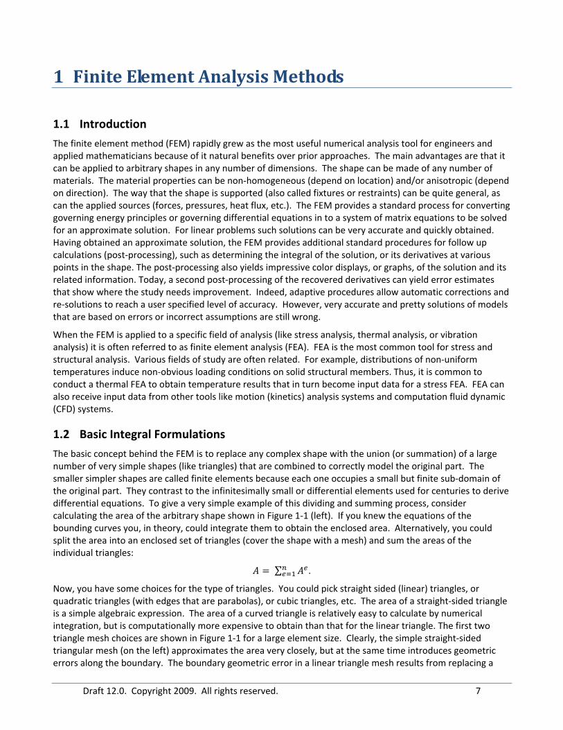
The basic concept behind the FEM is to replace any complex shape with the union (or summation) of a large number of very simple shapes (like triangles) that are combined to correctly model the original part. The smaller simpler shapes are called finite elements because each one occupies a small but finite sub‐domain of the original part. They contrast to the infinitesimally small or differential elements used for centuries to derive differential equations. To give a very simple example of this dividing and summing process, consider calculating the area of the arbitrary shape shown in Figure 1‐1 (left). If you knew the equations of the bounding curves you, in theory, could integrate them to obtain the enclosed area. Alternatively, you could split the area into an enclosed set of triangles (cover the shape with a mesh) and sum the areas of the individual triangles:

∑ .

Now, you have some choices for the type of triangles. You could pick straight sided (linear) triangles, or quadratic triangles (with edges that are parabolas), or cubic triangles, etc. The area of a straight‐sided triangle is a simple algebraic expression. The area of a curved triangle is relatively easy to calculate by numerical integration, but is computationally more expensive to obtain than that for the linear triangle. The first two triangle mesh choices are shown in Figure 1‐1 for a large element size. Clearly, the simple straight‐sided triangular mesh (on the left) approximates the area very closely, but at the same time introduces geometric errors along the boundary. The boundary geometric error in a linear triangle mesh results from replacing a

FEA Concepts: SW Simulation Overview J.E. Akin


boundary curve by a series of straight line segments. That geometric boundary error can be reduced to any desired level by increasing the number of linear triangles. But that decision increases the number of calculations and makes you trade off geometric accuracy versus the total number of required area calculations and summations.

Area is a scalar, so it makes sense to be able to simply sum its parts to determine the total value, as shown above. Other topics, like kinetic energy or strain energy, can be summed in the same fashion. Indeed, the very first applications of FEA to structures was based on minimizing the energy stored is a linear elastic material. The FEM always involves some type of governing integral statement. That integration is also converted to the sum of the integrals over each element in the mesh. Even if you start with a governing differential equation, it gets converted to an equivalent integral formulation by one of the methods of weighted residuals (MWR). The two most common methods, for FEA, are the Galerkin Method and the Method of Least Squares Figure.

Figure 1‐1 An area crudely meshed with linear and quadratic triangles

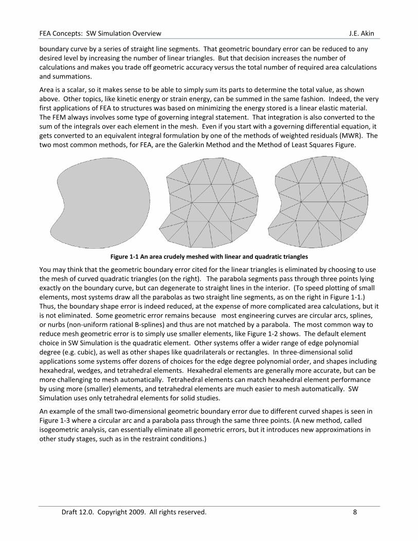
You may think that the geometric boundary error cited for the linear triangles is eliminated by choosing to use the mesh of curved quadratic triangles (on the right). The parabola segments pass through three points lying exactly on the boundary curve, but can degenerate to straight lines in the interior. (To speed plotting of small elements, most systems draw all the parabolas as two straight line segments, as on the right in Figure 1‐1.) Thus, the boundary shape error is indeed reduced, at the expense of more complicated area calculations, but it is not eliminated. Some geometric error remains because most engineering curves are circular arcs, splines, or nurbs (non‐uniform rational B‐splines) and thus are not matched by a parabola. The most common way to reduce mesh geometric error is to simply use smaller elements, like Figure 1‐2 shows. The default element choice in SW Simulation is the quadratic element. Other systems offer a wider range of edge polynomial degree (e.g. cubic), as well as other shapes like quadrilaterals or rectangles. In three‐dimensional solid applications some systems offer dozens of choices for the edge degree polynomial order, and shapes including hexahedral, wedges, and tetrahedral elements. Hexahedral elements are generally more accurate, but can be more challenging to mesh automatically. Tetrahedral elements can match hexahedral element performance by using more (smaller) elements, and tetrahedral elements are much easier to mesh automatically. SW Simulation uses only tetrahedral elements for solid studies.

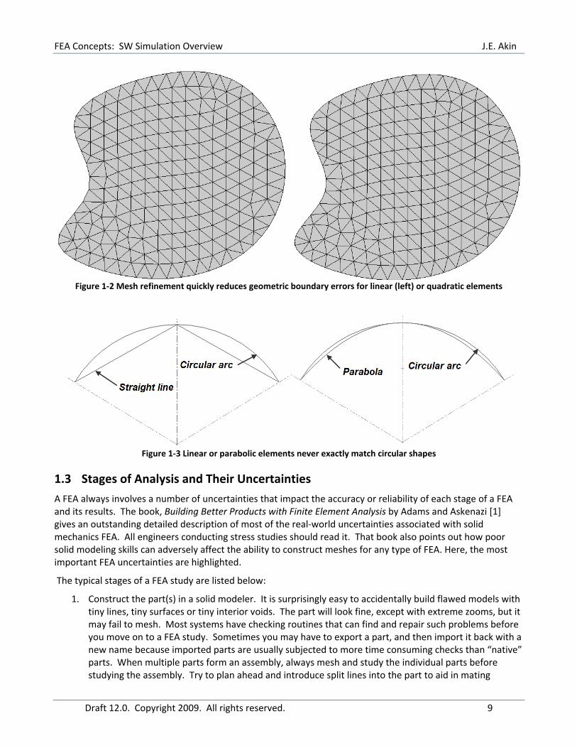
An example of the small two‐dimensional geometric boundary error due to different curved shapes is seen in Figure 1‐3 where a circular arc and a parabola pass through the same three points. (A new method, called isogeometric analysis, can essentially eliminate all geometric errors, but it introduces new approximations in other study stages, such as in the restraint conditions.)



Figure 1‐2 Mesh refinement quickly reduces geometric boundary errors for linear (left) or quadratic elements

Figure 1‐3 Linear or parabolic elements never exactly match circular shapes

1.3 Stages of Analysis and Their Uncertainties

A FEA always involves a number of uncertainties that impact the accuracy or reliability of each stage of a FEA and its results. The book, Building Better Products with Finite Element Analysis by Adams and Askenazi [1] gives an outstanding detailed description of most of the real‐world uncertainties associated with solid mechanics FEA. All engineers conducting stress studies should read it. That book also points out how poor solid modeling skills can adversely affect the ability to construct meshes for any type of FEA. Here, the most important FEA uncertainties are highlighted.

The typical stages of a FEA study are listed below:

1. Construct the part(s) in a solid modeler. It is surprisingly easy to accidentally build flawed models with tiny lines, tiny surfaces or tiny interior voids. The part will look fine, except with extreme zooms, but it may fail to mesh. Most systems have checking routines that can find and repair such problems before you move on to a FEA study. Sometimes you may have to export a part, and then import it back with a new name because imported parts are usually subjected to more time consuming checks than “native” parts. When multiple parts form an assembly, always mesh and study the individual parts before studying the assembly. Try to plan ahead and introduce split lines into the part to aid in mating



assemblies and to locate load regions and restraint (or fixture or support) regions. Today, construction of a part is probably the most reliable stage of any study.

2. Defeature the solid part model for meshing. The solid part may contain features, like a raised logo, that are not necessary to manufacture the part, or required for an accurate analysis study. They can be omitted from the solid used in the analysis study. That is a relative easy operation supported by most solid modelers (such as the “suppress” option in SW) to help make smaller and faster meshes. However, it has the potential for introducing serious, if not fatal, errors in a following engineering study. This is a reliable modeling process, but its application requires engineering judgment. For example, removing small radius interior fillets can greatly reduces the number of elements and simplifies the mesh generation. But, that creates sharp reentrant corners that can yield false infinite stresses. Those false high stress regions may cause you to overlook other areas of true high stress levels. Small holes lead to many small elements (and long run times). They also cause stress concentrations that raise the local stress levels by a factor of three. The decision to defeature them depends on where they are located in the part. If they lie in a high stress region you must keep them. But defeaturing them is allowed if you know they occur in a low stress region. Such decisions are complicated because most parts have multiple possible loading conditions (load cases) and a low stress region for one load case may become a high stress region for another load case.

3. Combine multiple parts into an assembly. Again, this is well automated and reliable from the geometric point of view and assemblies “look” as expected. However, geometric mating of part interfaces is very different for defining their physical (displacement, or temperature) mating. The physical mating choices are often unclear and the engineer may have to make a range of assumptions, study each, and determine the worst case result. Having to use physical contacts makes the linear problem require iterative solutions that take a long time to run and might fail to converge.

4. Select the element type. Some FEA systems have a huge number of available element types (with underlying theoretical restrictions). The SolidWorks system has only the fundamental types of elements. Namely, truss elements (bars), frame elements (beams), thin shells (or flat plates), thick shells, and solids. The system selects the element type (beginning in 2009) based on the shape of the part. The user is allowed to covert a non‐solid element region to a solid element region, and visa versa. Knowing which class of element will give a more accurate or faster solution requires training in finite element theory. At times a second element type study is used to help validate a study based on what is thought to be the best element type.

5. Mesh the part(s) or assembly, remembering that the mesh solid may not be the same as the part solid. A general rule in FEA is that your computer never has enough speed or memory. Sooner or later you will find a study that you cannot execute. Often that means you must utilize a crude mesh (or at least crude in some region) and/or invoke the use of symmetry or anti‐symmetry conditions. Local solution errors in a study are proportional to the product of the element size and the gradient of the secondary variables (i.e., gradient of stress or heat flux). Therefore, you exercise mesh control to place small elements where your engineering judgment estimates high stress (or flux) regions, as well as large elements in low stress regions. The local solution error also depends on the relative sizes of adjacent elements. You do not want skinny elements adjacent to big ones. Thus, automatic mesh generators have options to gradually vary adjacent element sizes from smallest to biggest.

The solid model sent to the mesh generator frequently should have load or restraint (fixture) regions formed by split lines, even if such splits are not needed for manufacturing the parts. The mesh typically should have refinements at source or load regions and support regions.

A mesh must look like the part, but that is not sufficient for a correct study. A single layer of elements filling a part region is almost never enough. If the region is curved, or subjected to bending, you want



at least three layers of quadratic elements, but five is a desirable lower limit. For linear elements you at least double those numbers.

Most engineers do not have access to the source code of their automatic mesh generator. When the mesher fails you frequently do not know why it failed or what to do about it. Often you have to re‐try the mesh generation with very large element sizes in hopes of getting some mesh results that can give hints as to why other attempts failed. The meshing of assemblies often fails. Usually the mesher runs out of memory because one or more parts had a very small, often unseen, feature that causes a huge number of tiny elements to be created. You should always attempt to mesh each individual part to spot such problems before you attempt to mesh them as a member of an assembly.

Automatic meshing, with mesh controls, is usually simple and fast today. However, it is only as reliable as the modified part or assembly supplied to it. Distorted elements usually do not develop in automatic mesh generators, due to empirical rules for avoiding them. However, distorted elements locations can usually be plotted. If they are in regions of low gradients you can usually accept them.

You should also note that studies involving natural frequencies are influenced most by the distribution of the mass of the part. Thus, they can still give accurate results with meshes that are much cruder than those that would be acceptable for stress or thermal studies.

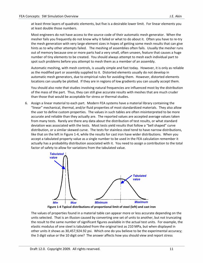
6. Assign a linear material to each part. Modern FEA systems have a material library containing the “linear” mechanical, thermal, and/or fluid properties of most standardized materials. They also allow the user to define custom properties. The values in such tables are often misinterpreted to be more accurate and reliable than they actually are. The reported values are accepted average values taken from many tests. Rarely are there any data about the distribution of test results, or what standard deviation was associated with the tests. Most tests yield results that follow a “bell shaped” curve distribution, or a similar skewed curve. The tests for stainless steel tend to have narrow distributions, like that on the left in Figure 1‐4, while the results for cast iron have wider distributions. When you accept a tabulated property value as a single number to be used in the FEA calculation remember it actually has a probability distribution associated with it. You need to assign a contribution to the total factor of safety to allow for variations from the tabulated value.

Figure 1‐4 Typical distributions of proportional limit of steel (left) and cast iron

The values of properties found in a material table can appear more or less accurate depending on the units selected. That is an illusion caused by converting one set of units to another, but not truncating the result to the same number of significant figures available in the actual test units. For example, the elastic modulus of one steel is tabulated from the original test as 210 MPa, but when displayed in other units it shows as 30,457,924.92 psi. Which one do you believe to be the experimental accuracy; the 3 digit value or the 10 digit one? The answer affects how you should view and report stress



results. The axial stress in a bar is equal to the elastic modulus times the strain, . Thus, if E is only known to three or four significant figures then the reported stress result should have no more significant figures. (It is true that the computer uses many digits to obtain the most accurate answer, but you should not accept the displayed numbers blindly.)

Material data are usually more reliable than the loading values (considered next), but less accurate that the model or mesh geometries.

7. Select regions of the part(s) to be loaded and assign load levels and load types to each region. In mathematical terminology, load or flux conditions on a boundary region are called Neumann boundary conditions, or non‐essential conditions. The geometric regions can be points (in theory), lines, surfaces, or volumes. If they are not existing features of the part, then you should apply split lines to the part to create them before activating the mesh generator. Point forces, or heat sources, are common in undergraduate studies, but in a FEA they cause false infinite stresses, or heat flux. If you include them do not be mislead by the high local values. Refining the mesh does not help much since the smallest element still reports near infinite values. In reality, point loads are better modeled as a total force, or pressure, acting over a small area formed by prior split lines.

Saint Venant’s Principle states that two different, but statically equivalent, force systems acting on a small portion of the surface of a body produce the same stress distributions at distantness large in comparison with the linear dimensions of the portion where the forces act. In undergraduate statics and dynamics courses engineers are taught to think in terms of point forces and couples. Solid elements do not accept pure couples as loads, but statically equivalent pressures can be applied to solids and yield the correct stresses. Indeed, a couple at a point is almost impossible to create, so the distribution of pressures is probably more like the true situation.

The magnitudes of applied loads are often guesses, or specified by a governing design standard. For example, consider a wind load. A building standard may quote a pressure to be applied for a given wind speed. But, how well do you know the wind speed that might actually be exerted on the structure? Again, there probably is some type of “bell curve” around the expected average speed. You need to assign a contribution to the total factor of safety to allow for variations in the uncertainty of the load value or actual spatial distribution of applied loads.

Loading data are usually less accurate than the material data, but much more accurate that the restraint or supporting conditions considered next.

8. Determine (or more likely assume) how the model interacts with the surroundings not included in your model. These are the restraint (support, or fixture) regions. In mathematical terminology, these are called the essential boundary conditions, or Dirichlet boundary conditions. You cannot afford to model everything interacting with a part. For many decades engineers have developed simplified concepts to approximate surroundings adjacent to a model to simplify hand calculations. They include roller supports, smooth pins, cantilevered (encastre, or fixed) supports, straight cable attachments, etc. Those concepts are often carried over to FEA approaches and can over simplify the true support nature and lead to very large errors in the results.

The choice of restraints (fixations, supports) for a model is surprisingly difficult and is often the least reliable decision made by the engineer. Small changes in the supports can cause large changes in the results. It is wise to try to investigate a number of likely or possible support conditions in different studies. When in doubt, try to include more of the surrounding support material and apply assumed support conditions to those portions at a greater distance from critical part features.

You need to assign a contribution to the total factor of safety to allow for variations in the uncertainty of how or where the actual support conditions occur.



9. Solve the linear system of equations, or the eigenvalue problem. With today’s numerical algorithms the solution of the algebraic system or eigen‐system is usually quite reliable. It is possible to cause ill‐conditioned systems (large condition number) with meshes having large elements adjacent to small ones, but that is unlikely to happen with automatic mesh generators.

10. Check the results. Are the reactions at the supports equal and opposite to the sources you thought that you applied? Are the results consistent with the assumed linear behavior? The engineering definition of a problem with large displacements is one where the maximum displacement is more than half the smallest geometric thickness of the part. The internal definition is a displacement field that significantly changes the volume of an element. That implies the element geometric shape noticeably changed from the starting shape, and that the shape needs to be updated in a series of much smaller shape changes. Are the displacements big enough to require re‐solution with large displacement iterations turned on? Have you validated the results with an analytic approximation, or different type of finite element? Engineering judgments are required.

11. Post‐process the solution for secondary variables. For structural studies you generally wish to document the deflections and stresses. For thermal studies you display the temperatures and heat flux vectors. With natural frequency models you show (or animate) a few mode shapes. You can control the number of contours employed, as well as their maximum and minimum ranges. The latter is important if you want to compare two designs on a single page. Limit the number of digits shown on the contour scale to be consistent with the material modulus (or conductivity, etc.). Contour plots often do not reproduce well in a report, but graphs generally do, so learn to include graphs in you documentation.

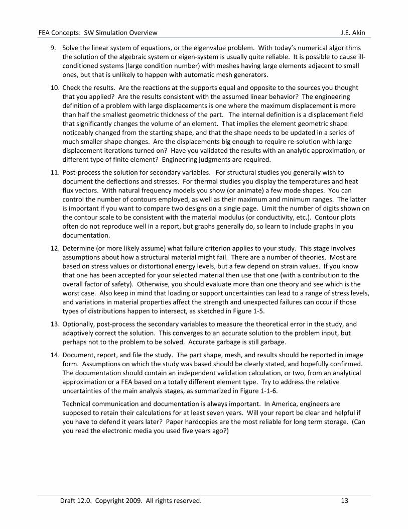
12. Determine (or more likely assume) what failure criterion applies to your study. This stage involves assumptions about how a structural material might fail. There are a number of theories. Most are based on stress values or distortional energy levels, but a few depend on strain values. If you know that one has been accepted for your selected material then use that one (with a contribution to the overall factor of safety). Otherwise, you should evaluate more than one theory and see which is the worst case. Also keep in mind that loading or support uncertainties can lead to a range of stress levels, and variations in material properties affect the strength and unexpected failures can occur if those types of distributions happen to intersect, as sketched in Figure 1‐5.

13. Optionally, post‐process the secondary variables to measure the theoretical error in the study, and adaptively correct the solution. This converges to an accurate solution to the problem input, but perhaps not to the problem to be solved. Accurate garbage is still garbage.

14. Document, report, and file the study. The part shape, mesh, and results should be reported in image form. Assumptions on which the study was based should be clearly stated, and hopefully confirmed. The documentation should contain an independent validation calculation, or two, from an analytical approximation or a FEA based on a totally different element type. Try to address the relative uncertainties of the main analysis stages, as summarized in Figure 1‐1‐6.

Technical communication and documentation is always important. In America, engineers are supposed to retain their calculations for at least seven years. Will your report be clear and helpful if you have to defend it years later? Paper hardcopies are the most reliable for long term storage. (Can you read the electronic media you used five years ago?)



Figure 1‐5 Distributions of loads/restraints and material strengths can cause failure

Figure 1‐1‐6 Relative uncertainty of major modeling stages

You usually assume that the materials are linear. If not (creeping, hyperelastic, inelastic, plastic, viscoelastic, etc.), define the appropriate material data and the nonlinear equations to be solved. Then the matrix system becomes non‐linear. Your original results check may lead you to conclude that the problem is actually an iterative one due to large displacements, or the need to insert physical contact interfaces.

1.4 Part Geometric Analysis and Meshing Failures

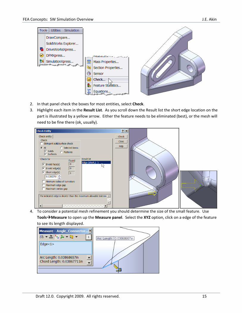
Before attempting meshing your part, for a finite element analysis, you should check your solid model for potentially fatal geometric flaws that may not be noticed except at greatly magnified views. Within SolidWorks this is called a Geometric Analysis. To utilise that feature, a geometric analysis check the Angel_Connector part will be outlined:

1. With the part open, go to Tools Check will open the Check Entity panel.



2. In that panel check the boxes for most entities, select Check. 3. Highlight each item in the Result List. As you scroll down the Result list the short edge location on the

part is illustrated by a yellow arrow. Either the feature needs to be eliminated (best), or the mesh will need to be fine there (ok, usually).

4. To consider a potential mesh refinement you should determine the size of the small feature. Use

Tools Measure to open up the Measure panel. Select the XYZ option, click on a edge of the feature to see its length displayed.



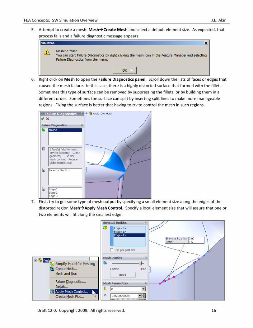
5. Attempt to create a mesh: Mesh Create Mesh and select a default element size. As expected, that process fails and a failure diagnostic message appears:

6. Right click on Mesh to open the Failure Diagnostics panel. Scroll down the lists of faces or edges that

caused the mesh failure. In this case, there is a highly distorted surface that formed with the fillets. Sometimes this type of surface can be removed by suppressing the fillets, or by building them in a different order. Sometimes the surface can split by inserting split lines to make more manageable regions. Fixing the surface is better that having to try to control the mesh in such regions.

7. First, try to get some type of mesh output by specifying a small element size along the edges of the

distorted region Mesh Apply Mesh Control. Specify a local element size that will assure that one or two elements will fit along the smallest edge.



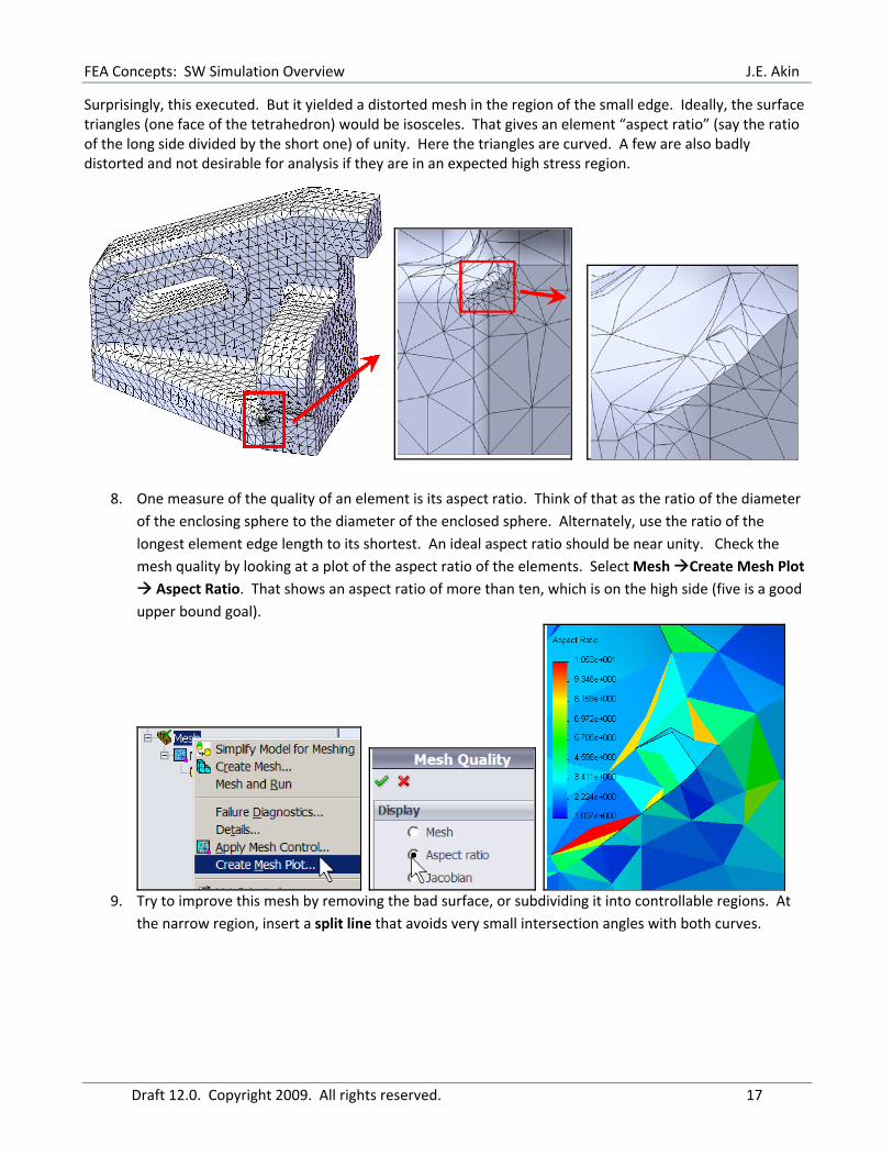
Surprisingly, this executed. But it yielded a distorted mesh in the region of the small edge. Ideally, the surface triangles (one face of the tetrahedron) would be isosceles. That gives an element “aspect ratio” (say the ratio of the long side divided by the short one) of unity. Here the triangles are curved. A few are also badly distorted and not desirable for analysis if they are in an expected high stress region.

8. One measure of the quality of an element is its aspect ratio. Think of that as the ratio of the diameter

of the enclosing sphere to the diameter of the enclosed sphere. Alternately, use the ratio of the longest element edge length to its shortest. An ideal aspect ratio should be near unity. Check the mesh quality by looking at a plot of the aspect ratio of the elements. Select Mesh Create Mesh Plot

Aspect Ratio. That shows an aspect ratio of more than ten, which is on the high side (five is a good upper bound goal).

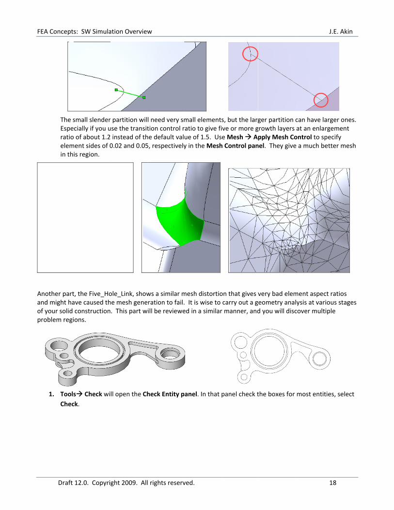
9. Try to improve this mesh by removing the bad surface, or subdividing it into controllable regions. At

the narrow region, insert a split line that avoids very small intersection angles with both curves.

FEA Concepts

Draft

The sEsperatioelemin th

Another partand might haof your solid problem regi

1. Tools

Chec

s: SW Simula

12.0. Copyri

small slendercially if you u of about 1.2

ment sides of 0is region.

t, the Five_Hoave caused thconstructionions.

s Check wick.

ation Overview

ght 2009. All

partition wiluse the transit instead of th0.02 and 0.05

ole_Link, showhe mesh gene. This part w

ll open the Ch

w

l rights reserv

l need very smtion control rhe default val5, respectively

ws a similar mration to fail.ill be reviewe

heck Entity p

ved.

mall elementratio to give fiue of 1.5. Usy in the Mesh

mesh distortio. It is wise to ed in a similar

panel. In that

s, but the largive or more gse Mesh Ah Control pan

on that gives carry out a gr manner, and

panel check t

ger partition growth layers pply Mesh Conel. They give

very bad elemeometry anad you will disc

the boxes for

J

1

can have largat an enlargeontrol to spece a much bett

ment aspect rlysis at varioucover multipl

most entities

.E. Akin

18

ger ones. ement cify ter mesh

ratios us stages e

s, select



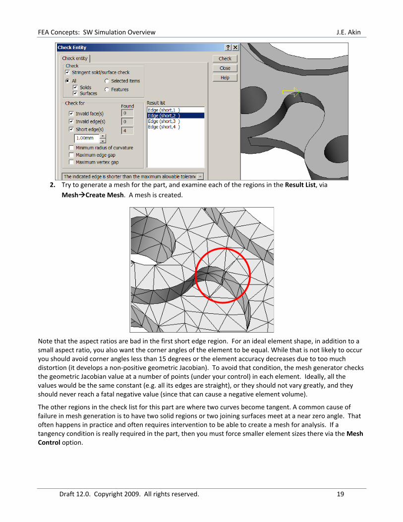
2. Try to generate a mesh for the part, and examine each of the regions in the Result List, via

Mesh Create Mesh. A mesh is created.

Note that the aspect ratios are bad in the first short edge region. For an ideal element shape, in addition to a small aspect ratio, you also want the corner angles of the element to be equal. While that is not likely to occur you should avoid corner angles less than 15 degrees or the element accuracy decreases due to too much distortion (it develops a non‐positive geometric Jacobian). To avoid that condition, the mesh generator checks the geometric Jacobian value at a number of points (under your control) in each element. Ideally, all the values would be the same constant (e.g. all its edges are straight), or they should not vary greatly, and they should never reach a fatal negative value (since that can cause a negative element volume).

The other regions in the check list for this part are where two curves become tangent. A common cause of failure in mesh generation is to have two solid regions or two joining surfaces meet at a near zero angle. That often happens in practice and often requires intervention to be able to create a mesh for analysis. If a tangency condition is really required in the part, then you must force smaller element sizes there via the Mesh Control option.

FEA Concepts

Draft

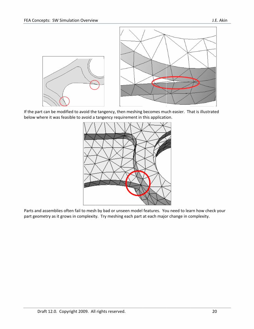
If the part cabelow where

Parts and asspart geometr

s: SW Simula

12.0. Copyri

n be modifiede it was feasib

semblies oftery as it grows

ation Overview

ght 2009. All

d to avoid theble to avoid a

n fail to meshs in complexit

w

l rights reserv

e tangency, thtangency req

h by bad or uty. Try meshi

ved.

hen meshing quirement in

nseen model ng each part

becomes muthis applicati

features. Yoat each majo

uch easier. Thon.

ou need to leaor change in c

J

2

hat is illustrat

arn how checomplexity.

.E. Akin

20

ted

k your

1 finite element analysis methods - rice university finite element analysis methods 1.1 introduction...

Documents