1 last lecture path planning for a moving visibility graph cell decomposition potential field ...

1

Last lecture Path planning for a moving

Visibility graph Cell decomposition Potential field

Geometric preliminariesImplementing geometric primitives correctly and efficiently is tricky and requires careful thought.

NUS CS 5247 David Hsu

Configuration SpaceConfiguration Space

3

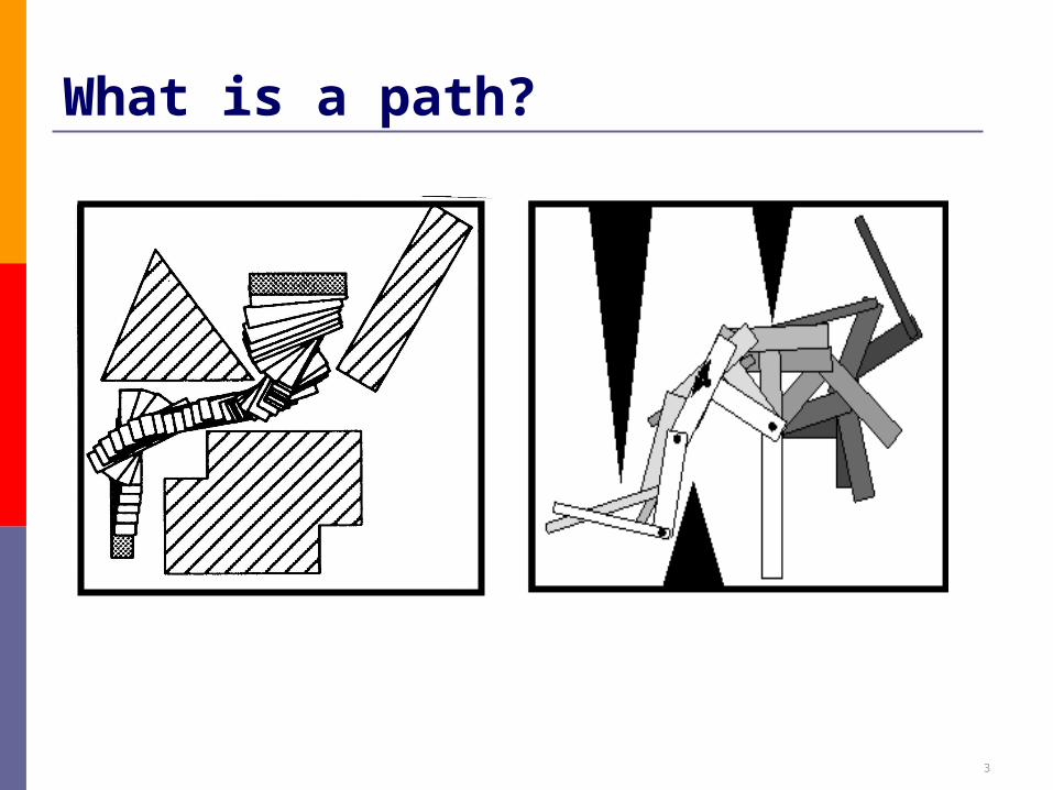
What is a path?

4

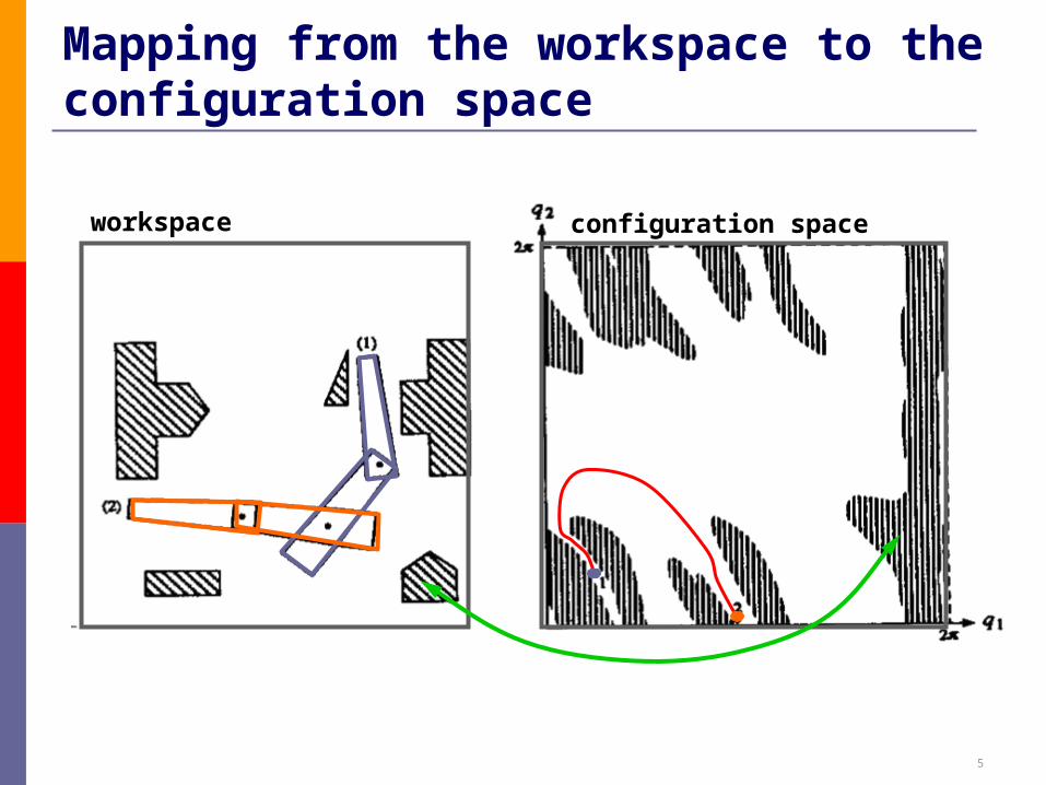
Rough idea Convert rigid robots, articulated robots, etc. into

points Apply algorithms for moving points

5

Mapping from the workspace to the configuration space

workspace configuration space

6

Configuration space Definitions and examples Obstacles Paths Metrics

7

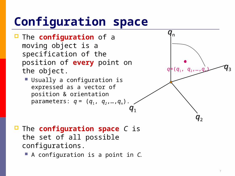
Configuration space The configuration of a moving

object is a specification of the position of every point on the object. Usually a configuration is expressed

as a vector of position & orientation parameters: q = (q1, q2,…,qn).

The configuration space C is the set of all possible configurations. A configuration is a point in C.

q=(q1, q2,…,qn)

qq11

qq22

qq33

qqnn

8

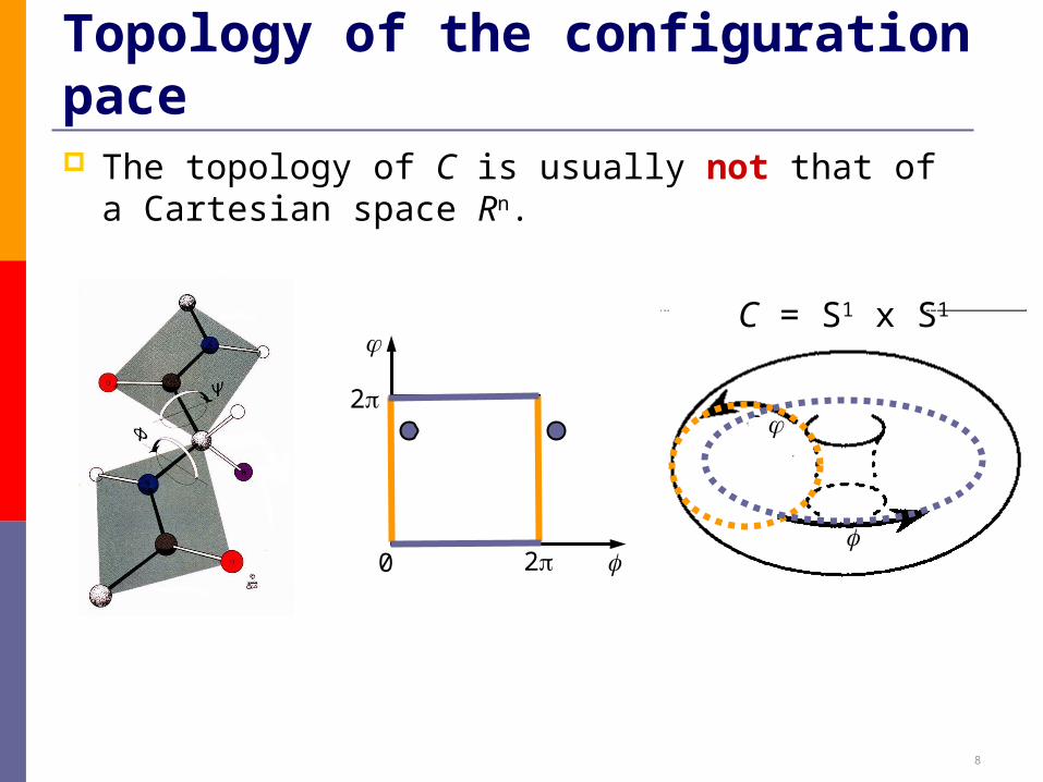
C = S1 x S1

Topology of the configuration pace The topology of C is usually not that of a Cartesian

space Rn.

0 2

2

9

Dimension of configuration space The dimension of a configuration space is the

minimum number of parameters needed to specify the configuration of the object completely.

It is also called the number of degrees of freedom (dofs) of a moving object.

10

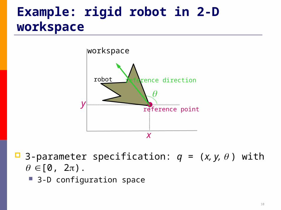
Example: rigid robot in 2-D workspace

3-parameter specification: q = (x, y, ) with [0, 2). 3-D configuration space

robot

workspace

reference point

x

y

reference direction

11

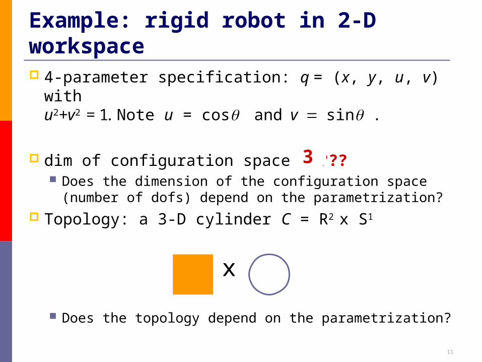
Example: rigid robot in 2-D workspace 4-parameter specification: q = (x, y, u, v) with

u2+v2 = 1. Note u = cosandvsin .

dim of configuration space = ??? Does the dimension of the configuration space

(number of dofs) depend on the parametrization? Topology: a 3-D cylinder C = R2 x S1

Does the topology depend on the parametrization?

3

x

12

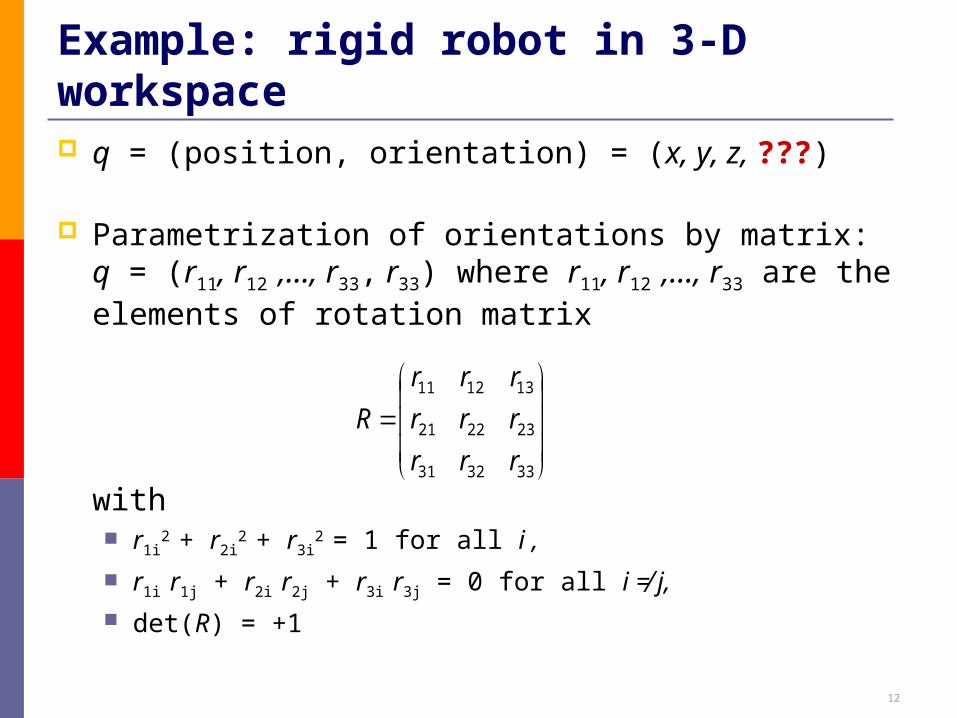
Example: rigid robot in 3-D workspace q = (position, orientation) = (x, y, z, ???)

Parametrization of orientations by matrix: q = (r11, r12 ,…, r33, r33) where r11, r12 ,…, r33 are the elements of rotation matrix

with r1i

2 + r2i2 + r3i

2 = 1 for all i ,

r1i r1j + r2i r2j + r3i r3j = 0 for all i ≠ j,

det(R) = +1

333231

232221

131211

rrr

rrr

rrr

R

13

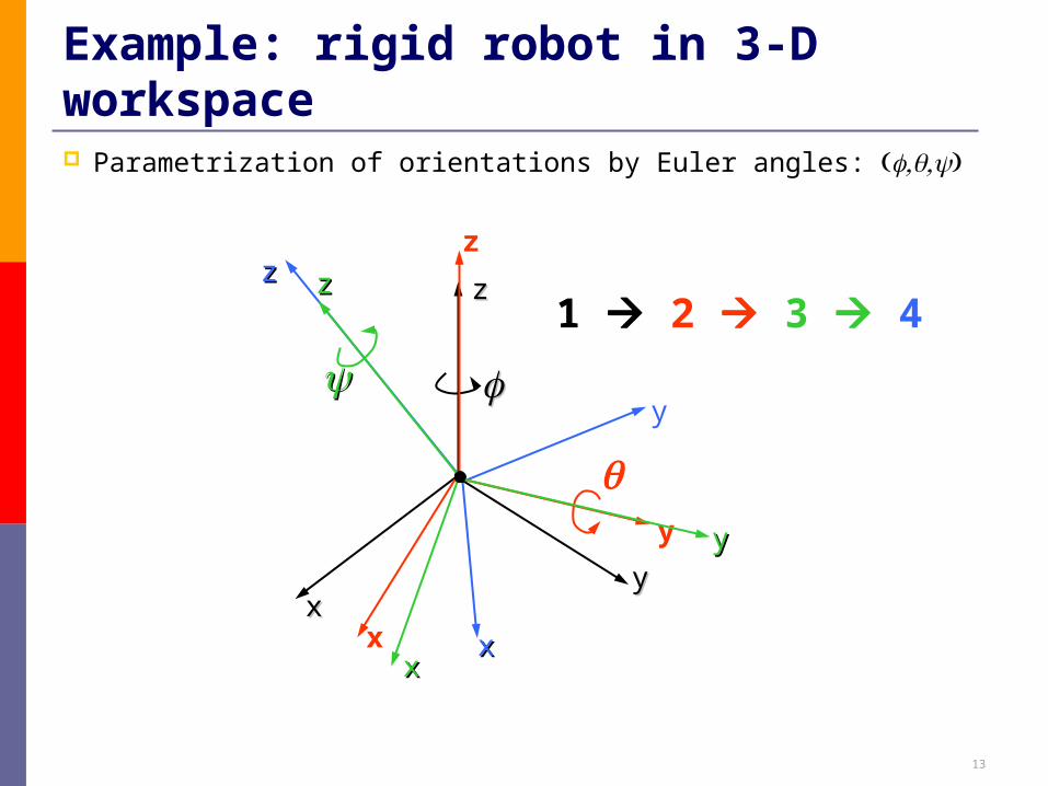
Example: rigid robot in 3-D workspace Parametrization of orientations by Euler angles:

xx

y

zz

xxyy

zz

x

y

z

xx

yy

zz

1 2 3 4

14

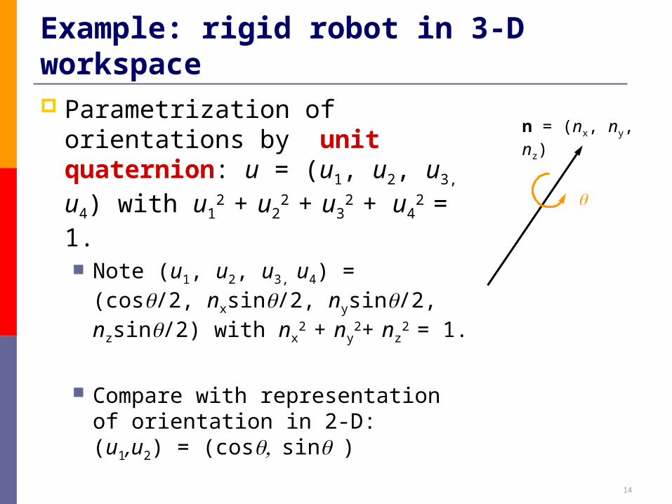
Parametrization of orientations by unit quaternion: u = (u1, u2, u3, u4) with u1

2 + u2

2 + u32 + u4

2 = 1. Note (u1, u2, u3, u4) =

(cos/2, nxsin/2, nysin/2, nzsin/2) with nx

2 + ny

2+ nz2 = 1.

Compare with representation of orientation in 2-D:(u1,u2) = (cossin)

Example: rigid robot in 3-D workspace

n = (nx, ny, nz)

15

Example: rigid robot in 3-D workspace Advantage of unit quaternion representation

Compact No singularity Naturally reflect the topology of the space of

orientations

Number of dofs = 6 Topology: R3 x SO(3)

16

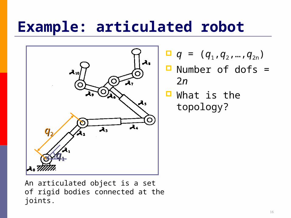
Example: articulated robot

q = (q1,q2,…,q2n)

Number of dofs = 2n What is the topology?

qq11

qq22

An articulated object is a set of rigid bodies connected at the joints.

17

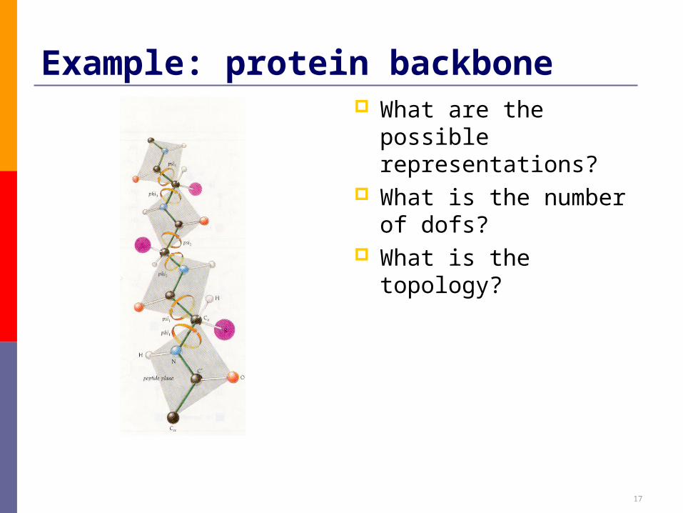
Example: protein backbone What are the possible

representations? What is the number of

dofs? What is the topology?

18


19

Obstacles in the configuration space A configuration q is collision-free, or free, if a

moving object placed at q does not intersect any obstacles in the workspace.

The free space F is the set of free configurations. A configuration space obstacle (C-obstacle) is

the set of configurations where the moving object collides with workspace obstacles.

20

Disc in 2-D workspace


workspace

21

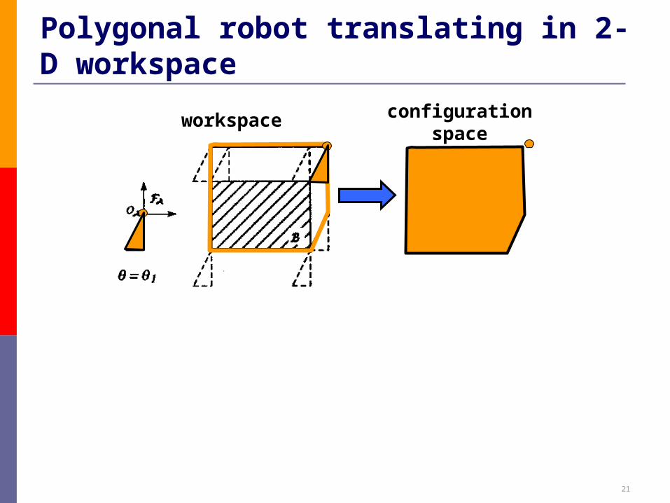
Polygonal robot translating in 2-D workspace


22

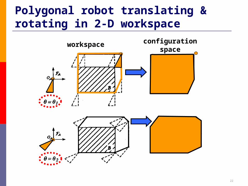
Polygonal robot translating & rotating in 2-D workspace


23

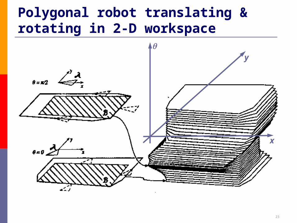
Polygonal robot translating & rotating in 2-D workspace

x

y

24

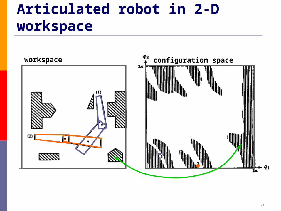
Articulated robot in 2-D workspace


25


26

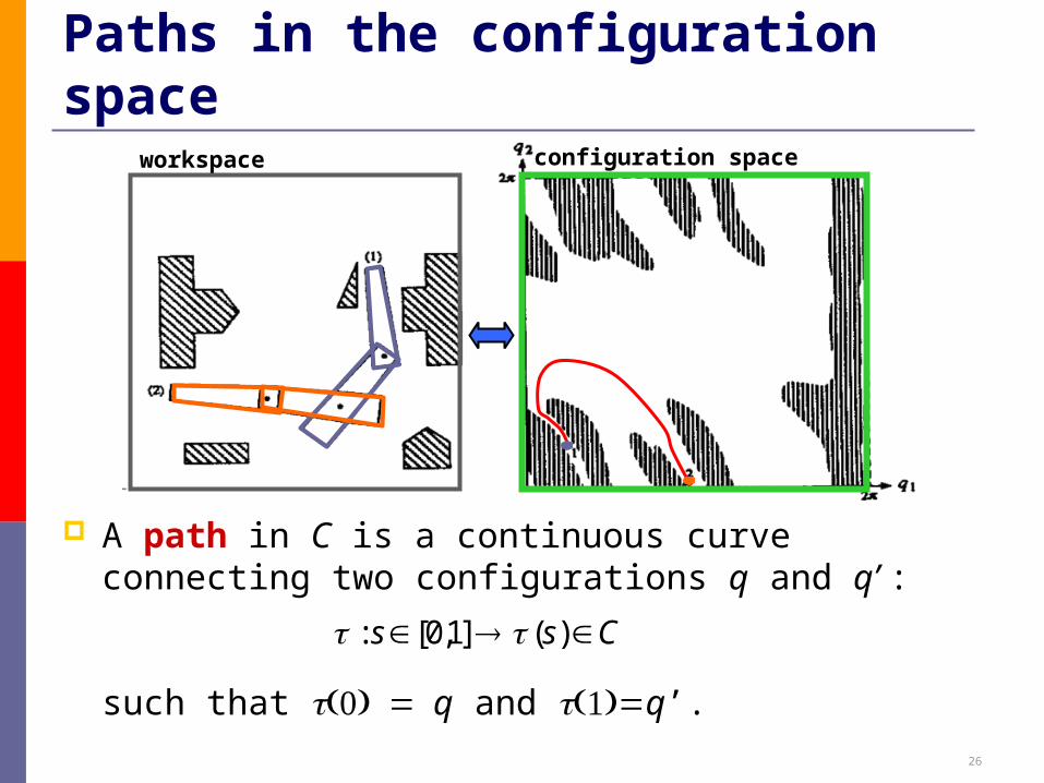
Paths in the configuration space

A path in C is a continuous curve connecting two configurations q and q’ :

such that q and q’.


Css )(]1,0[:

27

Constraints on paths

A trajectory is a path parameterized by time:

Constraints Finite length Bounded curvature Smoothness Minimum length Minimum time Minimum energy …

CtTt )(],0[:

28

Free space topology A free path lies entirely in the free space F. The moving object and the obstacles are

modeled as closed subsets, meaning that they contain their boundaries.

One can show that the C-obstacles are closed subsets of the configuration space C as well.

Consequently, the free space F is an open subset of C. Hence, each free configuration is the center of a ball of non-zero radius entirely contained in F.

29

Semi-free space A configuration q is semi-free if the moving

object placed q touches the boundary, but not the interior of obstacles. Free, or In contact

The semi-free space is a closed subset of C. Its boundary is a superset of the boundary of F.

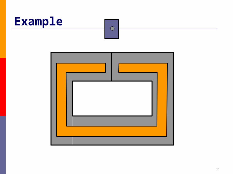
30

Example

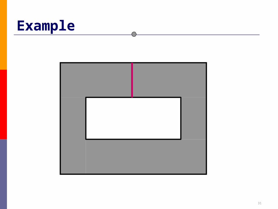
31

Example

32

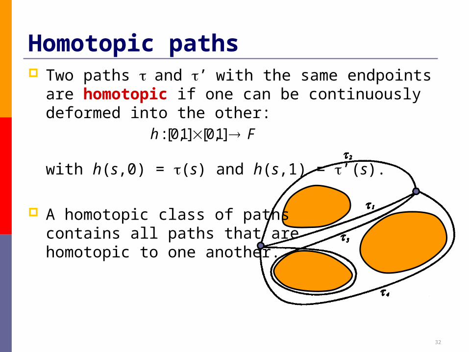
Two paths and ’with the same endpoints are homotopic if one can be continuously deformed into the other:

with h(s,0) = (s) and h(s,1) = ’(s).

A homotopic class of pathscontains all paths that arehomotopic to one another.

Homotopic paths

Fh ]1,0[]1,0[:

33

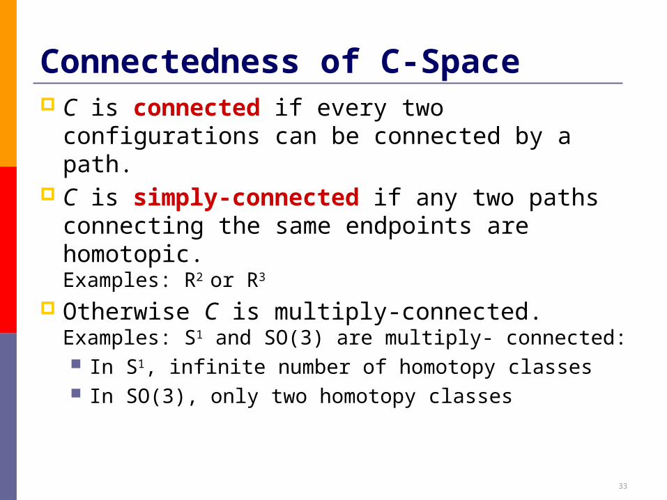
Connectedness of C-Space C is connected if every two configurations can

be connected by a path. C is simply-connected if any two paths

connecting the same endpoints are homotopic.Examples: R2 or R3

Otherwise C is multiply-connected.Examples: S1 and SO(3) are multiply- connected: In S1, infinite number of homotopy classes In SO(3), only two homotopy classes

34


35

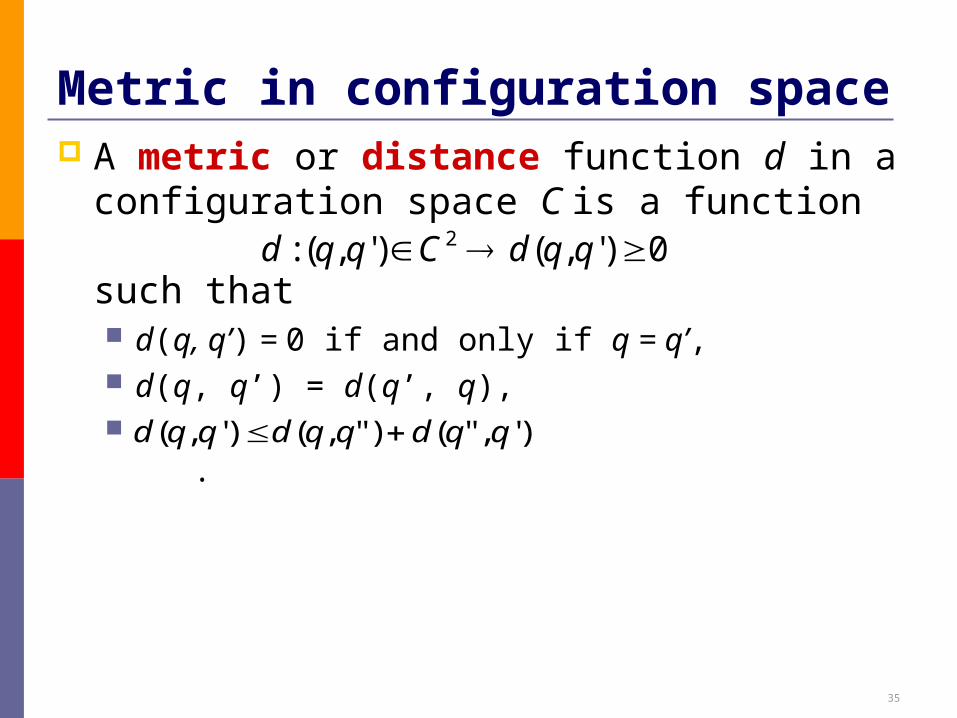
Metric in configuration space A metric or distance function d in a configuration

space C is a function

such that d(q, q’) = 0 if and only if q = q’, d(q, q’) = d(q’, q), .

0)',()',(: 2 qqdCqqd

)',"()",()',( qqdqqdqqd

36

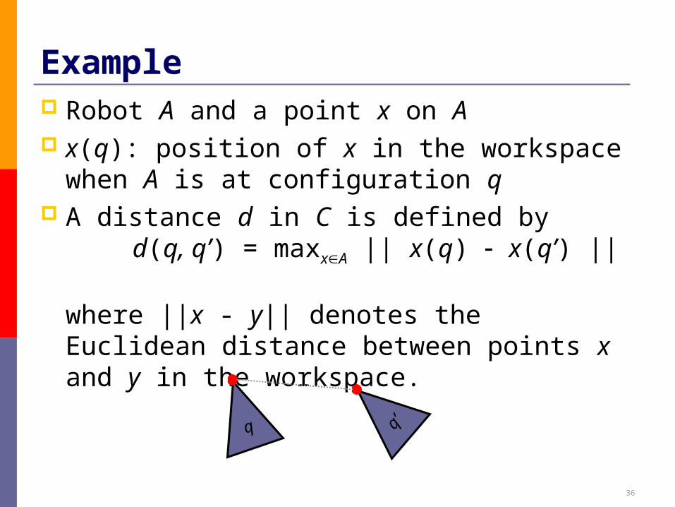
Example Robot A and a point x on A x(q): position of x in the workspace when A is at

configuration q A distance d in C is defined by

d(q, q’) = maxxA || x(q) x(q’) ||

where ||x - y|| denotes the Euclidean distance between points x and y in the workspace.

q q’

37

Examples in R2 x S1

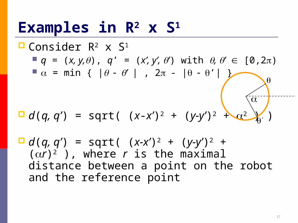
Consider R2 x S1

q = (x, y,), q’ = (x’, y’, ’) with , ’ [0,2) = min { |’| , 2- |’| }

d(q, q’) = sqrt( (x-x’)2 + (y-y’)2 + 2 ) )

d(q, q’) = sqrt( (x-x’)2 + (y-y’)2 + (r)2 ), where r is the maximal distance between a point on the robot and the reference point

’’

38

Summary on configuration space Parametrization Dimension (dofs) Topology Metric

NUS CS 5247 David Hsu

Minkowski SumMinkowski Sum

40

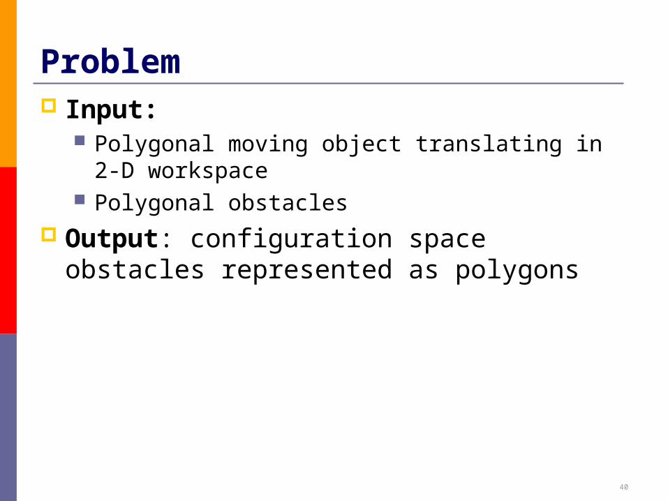
Problem Input:

Polygonal moving object translating in 2-D workspace Polygonal obstacles

Output: configuration space obstacles represented as polygons

41

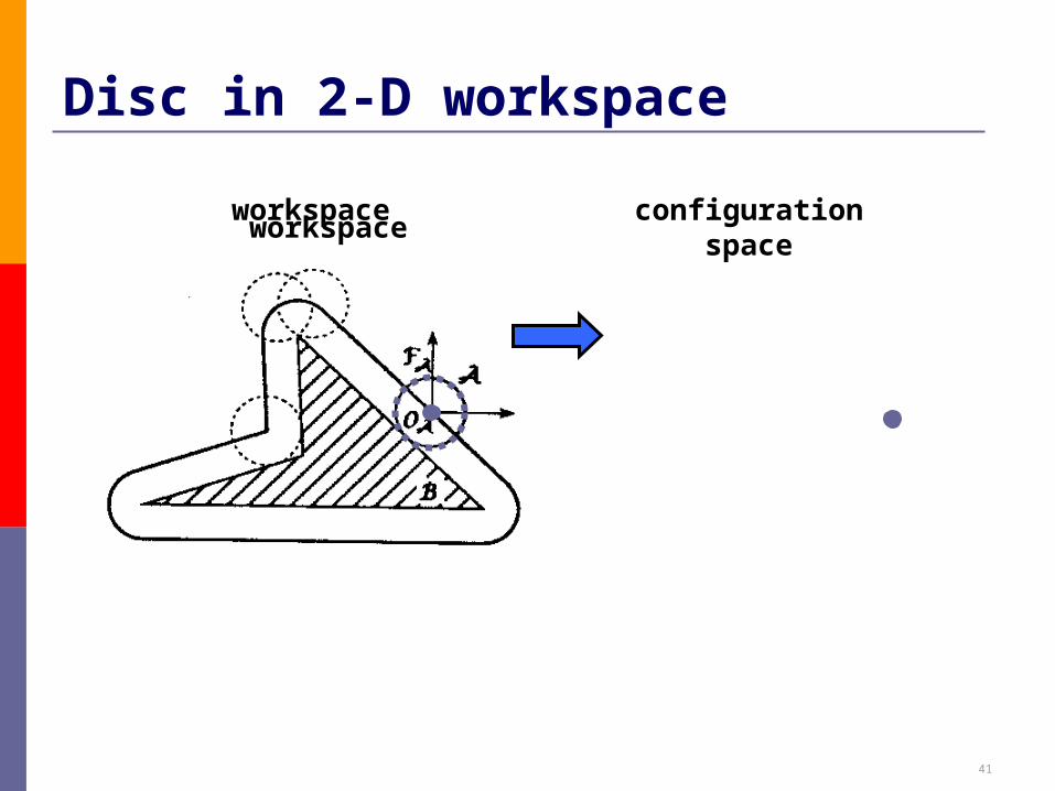
Disc in 2-D workspace


workspace

42

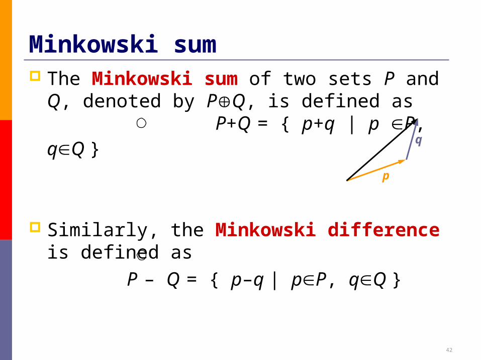
Minkowski sum The Minkowski sum of two sets P and Q,

denoted by PQ, is defined as P+Q = { p+q | p P, qQ }

Similarly, the Minkowski difference is defined as

P – Q = { p–q | pP, qQ }

p

q

43

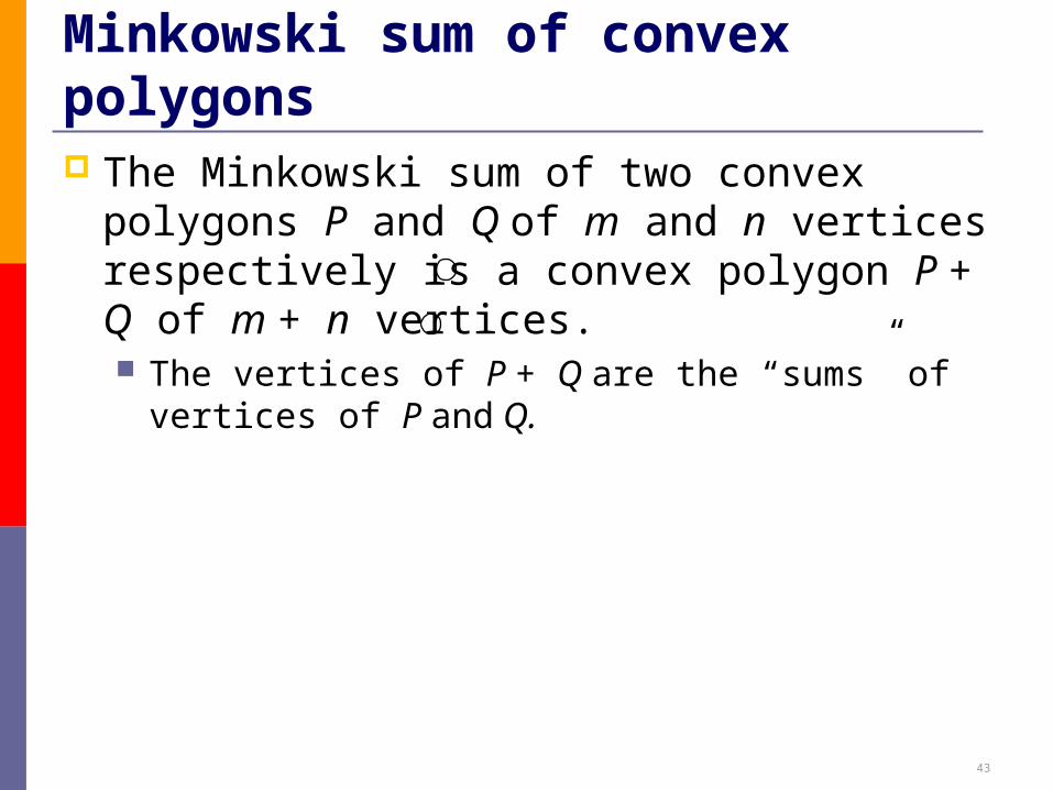
Minkowski sum of convex polygons The Minkowski sum of two convex polygons P

and Q of m and n vertices respectively is a convex polygon P + Q of m + n vertices. The vertices of P + Q are the “sums” of vertices of P

and Q.

44

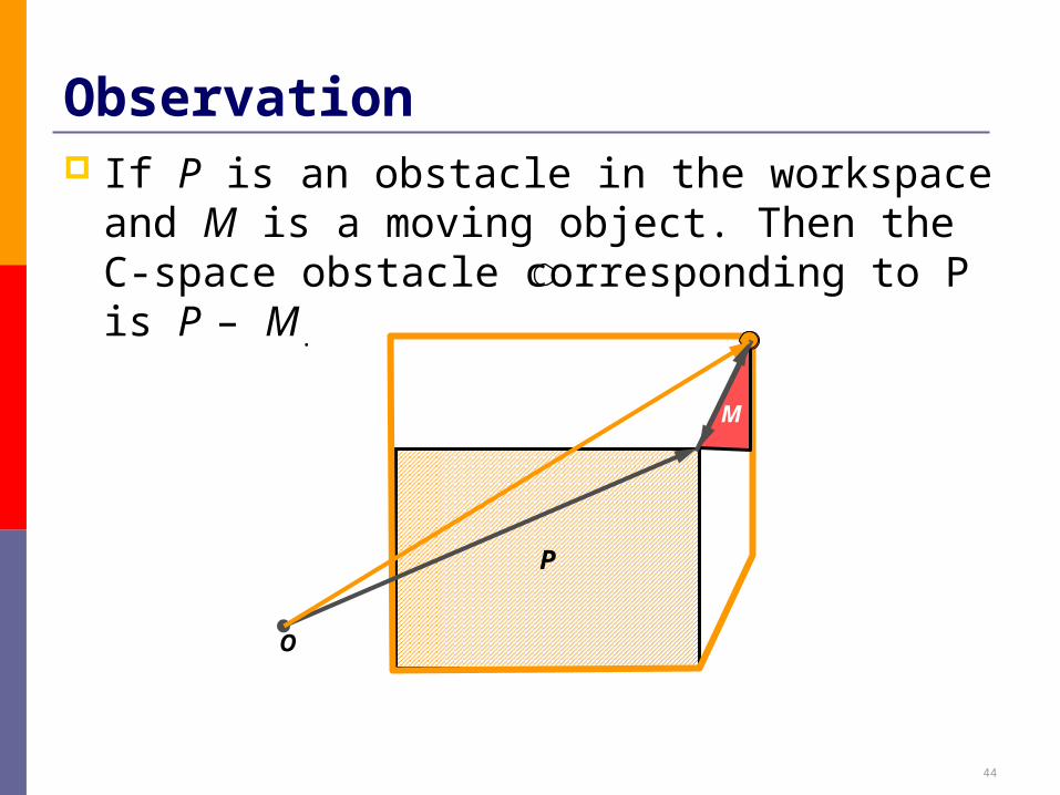
Observation If P is an obstacle in the workspace and M is a

moving object. Then the C-space obstacle corresponding to P is P – M.

P

M

O

45

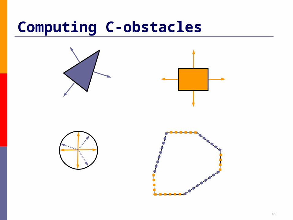
Computing C-obstacles

46

Computational efficiency Running time O(n+m) Space O(n+m) Non-convex obstacles

Decompose into convex polygons (e.g., triangles or trapezoids), compute the Minkowski sums, and take the union

Complexity of Minkowksi sum O(n2m2)

3-D workspace

1 last lecture path planning for a moving visibility graph cell decomposition potential field ...

Documents