15 partial derivatives - 國立臺灣大學cheng/teaching/ig_chapter15.pdf · chapter 15 partial...
TRANSCRIPT
15 PARTIAL DERIVATIVES
15.1 FUNCTIONS OF SEVERAL VARIABLES
TRANSPARENCIES AVAILABLE
#35 (Figure 10), #36 (Figure 13), #37 (Figure 17), #38 (Figure 19), #39 (Exercise 30), #40 (Exercises 51–56)
SUGGESTED TIME AND EMPHASIS
1 class Essential material
POINTS TO STRESS
1. A function of two or three variables is a rule assigning a real number to every point in its domain.
2. Functions of two variables can be represented as surfaces, and can be described in two dimensions by
contour maps and horizontal traces.
3. Functions of three variables can be described by level surfaces, and are generally more difficult to visualize
than functions of two variables.
QUIZ QUESTIONS
• Text Question: Why is the domain of the function in Example 4, g(x, y) =√9− x2 − y2, shaped like
a disk?
Answer: Because it is the region 9− x2 − y2 ≥ 0 or x2 + y2 ≤ 9
• Drill Question: If f is a function of two variables and f (3,−4) = −1, give the coordinates of a point
on the graph of f .
Answer: (3,−4,−1)
MATERIALS FOR LECTURE
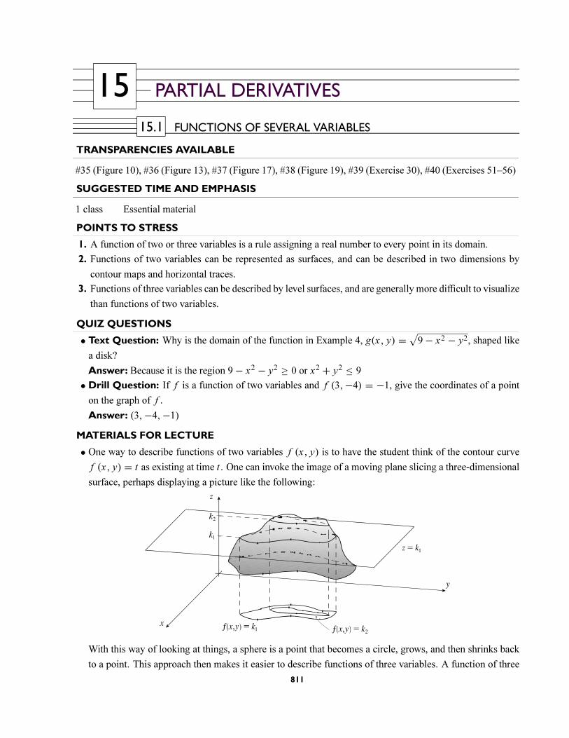
• One way to describe functions of two variables f (x, y) is to have the student think of the contour curve
f (x, y) = t as existing at time t . One can invoke the image of a moving plane slicing a three-dimensional
surface, perhaps displaying a picture like the following:
With this way of looking at things, a sphere is a point that becomes a circle, grows, and then shrinks back
to a point. This approach then makes it easier to describe functions of three variables. A function of three
811
CHAPTER 15 PARTIAL DERIVATIVES
variables can be thought of a level surface that changes with time. Example 15 can be revisited in this
context. f (x, y, z) = x2 + y2 + z2 can be pictured as a point at time t = 0, a sphere of radius 1 at time
t = 1, a sphere of radius√2 at t = 2, and so on. In other words, f (x, y, z) = x2 + y2 + z2 can be
pictured as a growing sphere, and the “level surfaces” of the function as snapshots of the process. Another
good function to describe with this method is f (x, y, z) = x2 + y2 − z.
• An alternate way to approach the subject is to think of one dimension as “color”. A surface such as
f (x, y) = sin x + cos y could be then drawn on a sheet of graph paper, with red representing the contour
curve f (x, y) = −2, violet representing the contour curve f (x, y) = 2, and any number in between
represented by the appropriate color. Some software packages represent functions of three variables using
a method similar to this one.
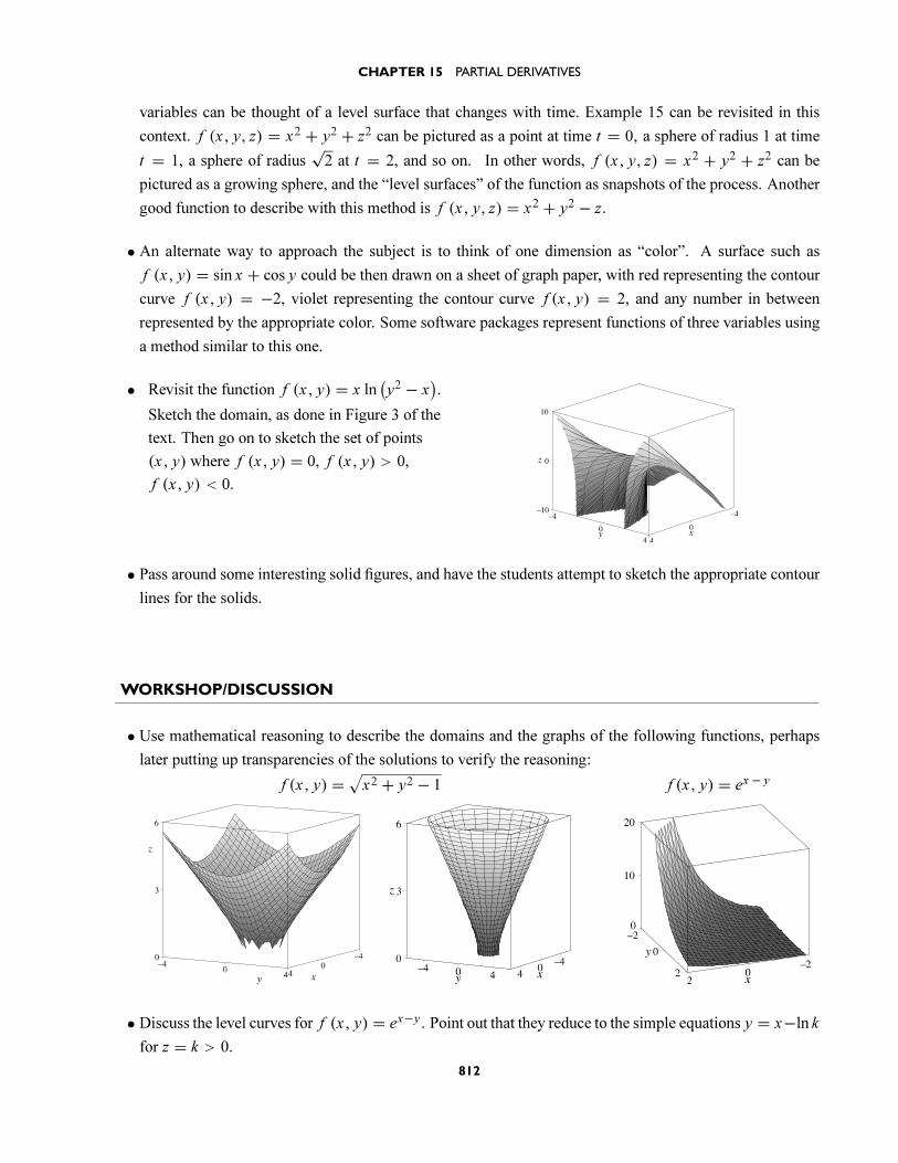
• Revisit the function f (x, y) = x ln(y2 − x
).
Sketch the domain, as done in Figure 3 of the
text. Then go on to sketch the set of points
(x, y) where f (x, y) = 0, f (x, y) > 0,
f (x, y) < 0.
• Pass around some interesting solid figures, and have the students attempt to sketch the appropriate contour
lines for the solids.
WORKSHOP/DISCUSSION
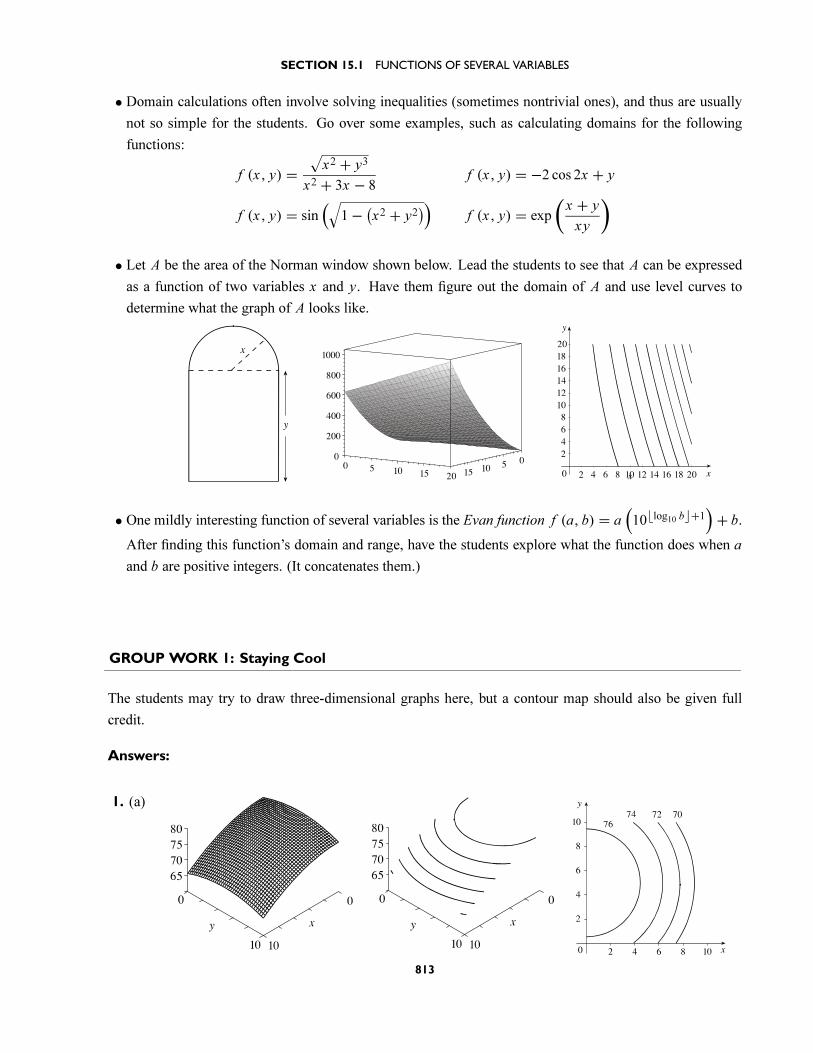
• Use mathematical reasoning to describe the domains and the graphs of the following functions, perhaps
later putting up transparencies of the solutions to verify the reasoning:
f (x, y) =√x2 + y2 − 1 f (x, y) = ex − y
• Discuss the level curves for f (x, y) = ex−y . Point out that they reduce to the simple equations y = x−ln k
for z = k > 0.
812
SECTION 15.1 FUNCTIONS OF SEVERAL VARIABLES
• Domain calculations often involve solving inequalities (sometimes nontrivial ones), and thus are usually
not so simple for the students. Go over some examples, such as calculating domains for the following
functions:
f (x, y) =√x2 + y3
x2 + 3x − 8f (x, y) = −2 cos 2x + y
f (x, y) = sin(√
1− (x2 + y2))
f (x, y) = exp
(x + y
xy
)
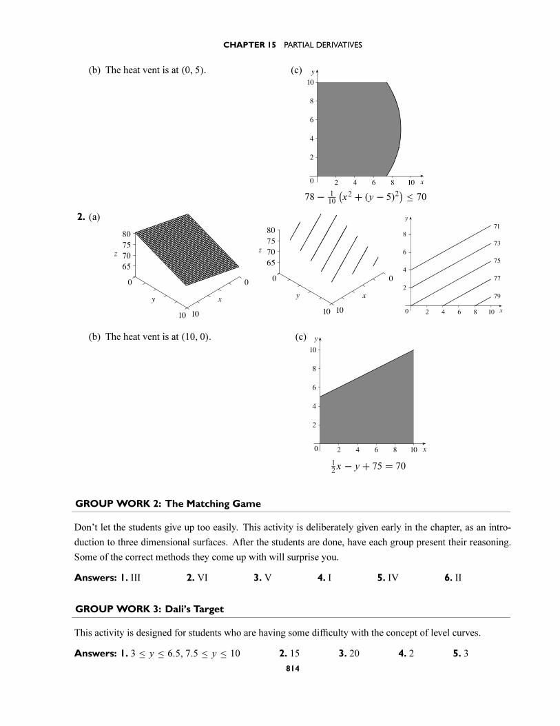
• Let A be the area of the Norman window shown below. Lead the students to see that A can be expressed
as a function of two variables x and y. Have them figure out the domain of A and use level curves to
determine what the graph of A looks like.
x
y
510
1520
0 5 10 15
0
200
400
600
800
1000
02
4
6
8
10
12
14
16
18
20
y
2 4 6 8 10 12 14 16 18 20x x0
• One mildly interesting function of several variables is the Evan function f (a, b) = a(10�log10 b�+1
)+ b.
After finding this function’s domain and range, have the students explore what the function does when a
and b are positive integers. (It concatenates them.)
GROUP WORK 1: Staying Cool
The students may try to draw three-dimensional graphs here, but a contour map should also be given full
credit.
Answers:
1. (a)
813
CHAPTER 15 PARTIAL DERIVATIVES
(b) The heat vent is at (0, 5). (c)
78− 110
(x2 + (y − 5)2
) ≤ 70
2. (a)
(b) The heat vent is at (10, 0). (c)
12x − y + 75 = 70
GROUP WORK 2: The Matching Game
Don’t let the students give up too easily. This activity is deliberately given early in the chapter, as an intro-
duction to three dimensional surfaces. After the students are done, have each group present their reasoning.
Some of the correct methods they come up with will surprise you.
Answers: 1. III 2. VI 3. V 4. I 5. IV 6. II
GROUP WORK 3: Dali’s Target
This activity is designed for students who are having some difficulty with the concept of level curves.
Answers: 1. 3 ≤ y ≤ 6.5, 7.5 ≤ y ≤ 10 2. 15 3. 20 4. 2 5. 3
814
SECTION 15.1 FUNCTIONS OF SEVERAL VARIABLES
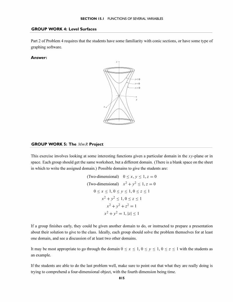
GROUP WORK 4: Level Surfaces
Part 2 of Problem 4 requires that the students have some familiarity with conic sections, or have some type of
graphing software.
Answer:
GROUP WORK 5: The MmR Project
This exercise involves looking at some interesting functions given a particular domain in the xy-plane or in
space. Each group should get the same worksheet, but a different domain. (There is a blank space on the sheet
in which to write the assigned domain.) Possible domains to give the students are:
(Two-dimensional) 0 ≤ x , y ≤ 1, z = 0
(Two-dimensional) x2 + y2 ≤ 1, z = 0
0 ≤ x ≤ 1, 0 ≤ y ≤ 1, 0 ≤ z ≤ 1
x2 + y2 ≤ 1, 0 ≤ z ≤ 1
x2 + y2 + z2 = 1
x2 + y2 = 1, |z| ≤ 1
If a group finishes early, they could be given another domain to do, or instructed to prepare a presentation
about their solution to give to the class. Ideally, each group should solve the problem themselves for at least
one domain, and see a discussion of at least two other domains.
It may be most appropriate to go through the domain 0 ≤ x ≤ 1, 0 ≤ y ≤ 1, 0 ≤ z ≤ 1 with the students as
an example.
If the students are able to do the last problem well, make sure to point out that what they are really doing is
trying to comprehend a four-dimensional object, with the fourth dimension being time.
815
CHAPTER 15 PARTIAL DERIVATIVES
EXTENDED GROUP PROJECT: Applied Contour Maps
Give the students a list of today’s temperature in various cities, along with a map of the country. The temper-
atures are available in many newspapers. Have the students draw a contour map showing curves of constant
temperature. Then give them a copy of the temperature contour map from a newspaper to compare with their
map to see how they did. Discuss what a three-dimensional representation of today’s weather would be like.
You can have the students cut the contours out of corrugated cardboard and make actual three-dimensional
weather maps.
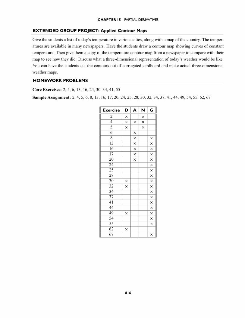
HOMEWORK PROBLEMS
Core Exercises: 2, 5, 6, 13, 16, 24, 30, 34, 41, 55
Sample Assignment: 2, 4, 5, 6, 8, 13, 16, 17, 20, 24, 25, 28, 30, 32, 34, 37, 41, 44, 49, 54, 55, 62, 67
Exercise D A N G
2 × ×4 × × ×5 × ×6 ×8 × ×13 × ×16 × ×17 × ×20 × ×24 ×25 ×28 ×30 × ×32 × ×34 ×37 ×41 ×44 ×49 × ×54 ×55 ×62 ×67 ×
816
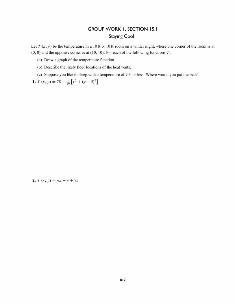
GROUP WORK 1, SECTION 15.1
Staying Cool
Let T (x, y) be the temperature in a 10 ft× 10 ft room on a winter night, where one corner of the room is at
(0, 0) and the opposite corner is at (10, 10). For each of the following functions T ,
(a) Draw a graph of the temperature function.
(b) Describe the likely floor locations of the heat vents.
(c) Suppose you like to sleep with a temperature of 70◦ or less. Where would you put the bed?
1. T (x, y) = 78− 110
[x2 + (y − 5)2
]
2. T (x, y) = 12x − y + 75
817
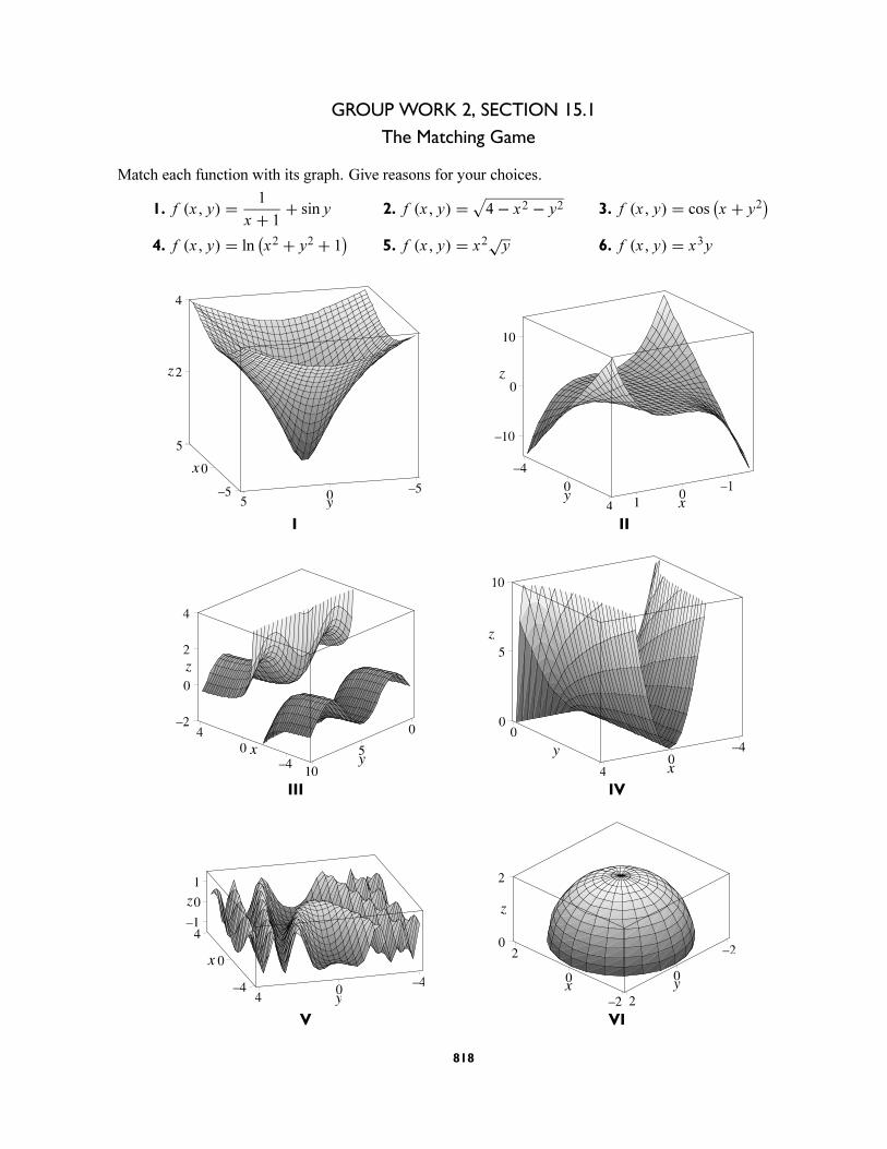
GROUP WORK 2, SECTION 15.1
The Matching Game
Match each function with its graph. Give reasons for your choices.
1. f (x, y) = 1
x + 1+ sin y 2. f (x, y) =
√4− x2 − y2 3. f (x, y) = cos
(x + y2
)4. f (x, y) = ln
(x2 + y2 + 1
)5. f (x, y) = x2
√y 6. f (x, y) = x3y
I II
III IV
V VI
818

GROUP WORK 3, SECTION 15.1
Dali’s Target
Consider the following contour map of a continuous function f (x, y):
1. For approximately what values of y is it true that 10 ≤ f (5, y) ≤ 30?
2. What can you estimate f (2, 4) to be, and why?
3. Do we have any good estimates for f (5, 8)? Explain.
4. How many values y satisfy f (7, y) = 20?
5. How many values of x satisfy f (x, 8) = 20?
819
GROUP WORK 4, SECTION 15.1
Level Surfaces
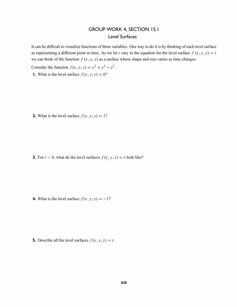
It can be difficult to visualize functions of three variables. One way to do it is by thinking of each level surface
as representing a different point in time. As we let t vary in the equation for the level surface f (x, y, z) = t
we can think of the function f (x, y, z) as a surface whose shape and size varies as time changes.
Consider the function f (x, y, z) = x2 + y2 − z2.
1. What is the level surface f (x, y, z) = 0?
2. What is the level surface f (x, y, z) = 1?
3. For t > 0, what do the level surfaces f (x, y, z) = t look like?
4. What is the level surface f (x, y, z) = −1?
5. Describe all the level surfaces f (x, y, z) = t .
820
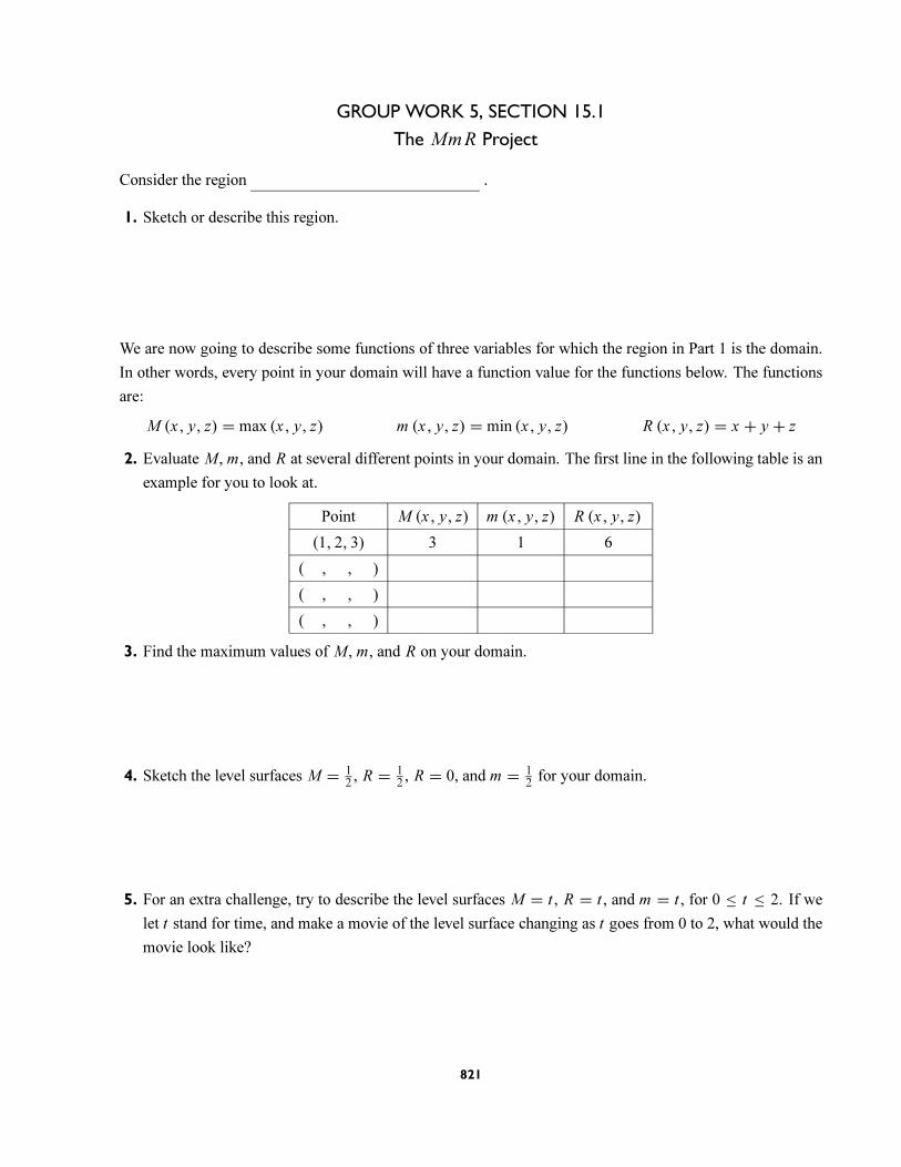
GROUP WORK 5, SECTION 15.1
The MmR Project
Consider the region .
1. Sketch or describe this region.
We are now going to describe some functions of three variables for which the region in Part 1 is the domain.
In other words, every point in your domain will have a function value for the functions below. The functions
are:
M (x, y, z) = max (x, y, z) m (x, y, z) = min (x, y, z) R (x, y, z) = x + y + z
2. Evaluate M , m, and R at several different points in your domain. The first line in the following table is an
example for you to look at.
Point M (x, y, z) m (x, y, z) R (x, y, z)
(1, 2, 3) 3 1 6
( , , )
( , , )
( , , )
3. Find the maximum values of M , m, and R on your domain.
4. Sketch the level surfaces M = 12, R = 1
2, R = 0, and m = 1
2for your domain.
5. For an extra challenge, try to describe the level surfaces M = t , R = t , and m = t , for 0 ≤ t ≤ 2. If we
let t stand for time, and make a movie of the level surface changing as t goes from 0 to 2, what would the
movie look like?
821
15.2 LIMITS AND CONTINUITY
SUGGESTED TIME AND EMPHASIS
1 class Recommended material. This material can be covered from a variety of perspectives, and at a
variety of depths. (For example, the nonexistence of certain limits can be de-emphasized.) The
instructor should feel especially free to pick and choose from the suggestions below.
POINTS TO STRESS
1. While the definitions of limits and continuity for multivariable functions are nearly identical to those of
their single variable counterparts, very different behavior can take place in the multivariable case.
2. The idea of points being “close” in R2 and R3.
QUIZ QUESTIONS
• Text Question: When talking about limits for functions of several variables, why isn’t it sufficient to say,
“ lim(x,y)→(0,0)
f (x, y) = L if f (x, y) gets close to L as we approach (0, 0) along the x-axis (y = 0) and
along the y-axis (x = 0)”?
Answer: Path independence is important, and only two paths are discussed above.
• Drill Question: Show that lim(x,y)→(0,0)
(x2 + y2
) = 0.
Answer: Any answer that correctly addresses path independence should be given credit.
MATERIALS FOR LECTURE
• Stress that f (x, y) → L as (x, y) → (a, b) means that f (x, y) gets as close to L as we like as (x, y)
gets close to (a, b) in distance, that is, regardless of path. Give examples of exotic paths to (0, 0) such as
the following:
x
y
x
y
x
y
x
y
• This is a rich example of a limit that exists:
lim(x,y)→(0,0)
sin(x2 + y2
)x2 + y2
= 1
Sincesin(x2 + y2
)x2 + y2
is constant on circles centered at the origin, we want to look at the distancew between
(x, y) and (0, 0): w =√x2 + y2. Computationally, it is best to look at what happens when w2 → 0. In
this case,sin(x2 + y2
)x2 + y2
= sinw2
w2, and single-variable calculus gives us that lim
w→0
sinw2
w2= 1. Stress that
in general it does not suffice to just let x = 0 or y = 0 and then compute the limit.
822
SECTION 15.2 LIMITS AND CONTINUITY
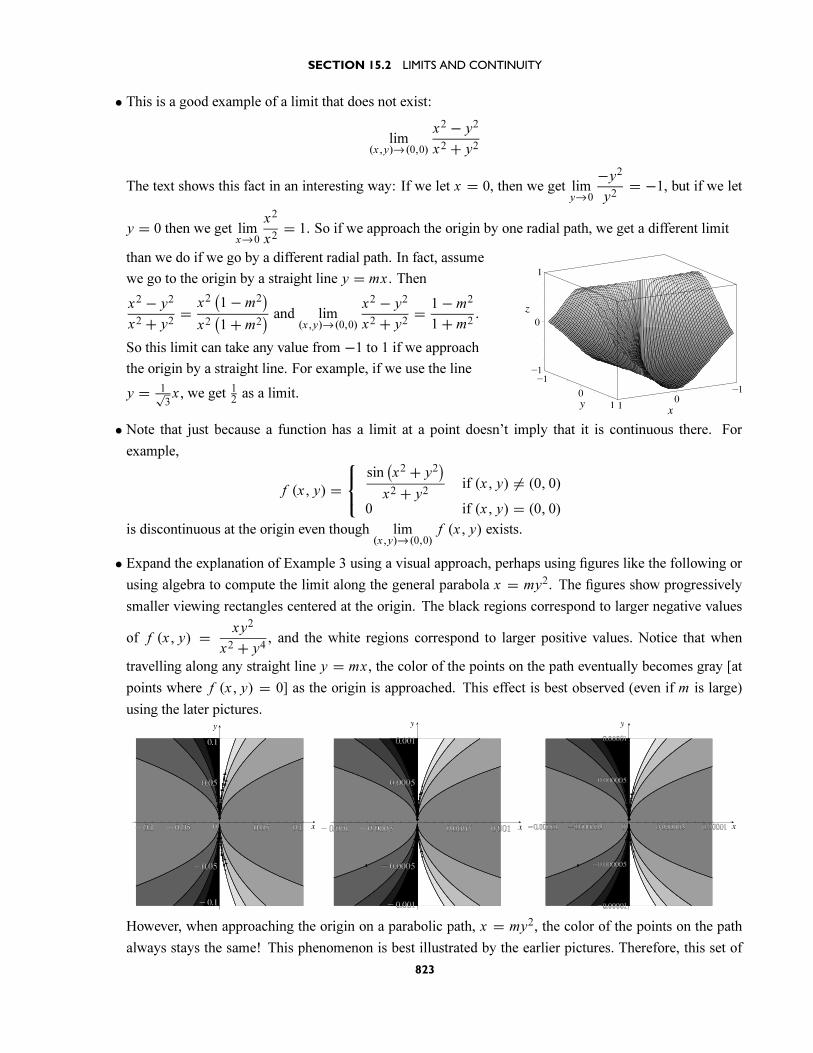
• This is a good example of a limit that does not exist:
lim(x,y)→(0,0)
x2 − y2
x2 + y2
The text shows this fact in an interesting way: If we let x = 0, then we get limy→0
−y2
y2= −1, but if we let
y = 0 then we get limx→0
x2
x2= 1. So if we approach the origin by one radial path, we get a different limit
than we do if we go by a different radial path. In fact, assume
we go to the origin by a straight line y = mx . Then
x2 − y2
x2 + y2= x2
(1− m2
)x2(1+ m2
) and lim(x,y)→(0,0)
x2 − y2
x2 + y2= 1− m2
1+ m2.
So this limit can take any value from −1 to 1 if we approach
the origin by a straight line. For example, if we use the line
y = 1√3x , we get 1
2as a limit.
• Note that just because a function has a limit at a point doesn’t imply that it is continuous there. For
example,
f (x, y) =⎧⎨⎩
sin(x2 + y2
)x2 + y2
if (x, y) = (0, 0)
0 if (x, y) = (0, 0)
is discontinuous at the origin even though lim(x,y)→(0,0)
f (x, y) exists.
• Expand the explanation of Example 3 using a visual approach, perhaps using figures like the following or
using algebra to compute the limit along the general parabola x = my2. The figures show progressively
smaller viewing rectangles centered at the origin. The black regions correspond to larger negative values
of f (x, y) = xy2
x2 + y4, and the white regions correspond to larger positive values. Notice that when
travelling along any straight line y = mx , the color of the points on the path eventually becomes gray [at
points where f (x, y) = 0] as the origin is approached. This effect is best observed (even if m is large)
using the later pictures.
However, when approaching the origin on a parabolic path, x = my2, the color of the points on the path
always stays the same! This phenomenon is best illustrated by the earlier pictures. Therefore, this set of
823
CHAPTER 15 PARTIAL DERIVATIVES
plots illustrates how the limit as (x, y) → (0, 0) of f (x, y) = xy2
x2 + y4does not exist, although one would
erroneously believe it to be 0 if one looked only at the “obvious” linear paths.
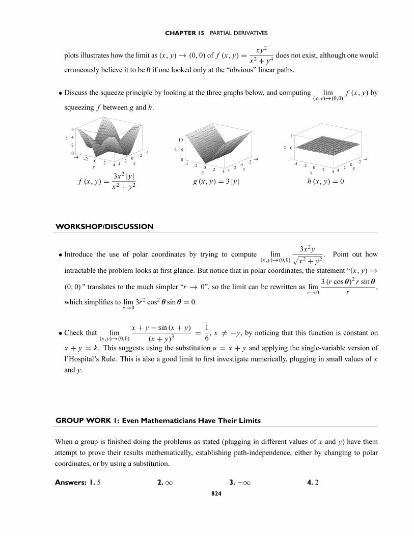
• Discuss the squeeze principle by looking at the three graphs below, and computing lim(x,y)→(0,0)
f (x, y) by
squeezing f between g and h.
f (x, y) = 3x2 |y|x2 + y2
g (x, y) = 3 |y| h (x, y) = 0
WORKSHOP/DISCUSSION
• Introduce the use of polar coordinates by trying to compute lim(x,y)→(0,0)
3x2y√x2 + y2
. Point out how
intractable the problem looks at first glance. But notice that in polar coordinates, the statement “(x, y) →
(0, 0) " translates to the much simpler “r → 0”, so the limit can be rewritten as limr→0
3 (r cosθ)2 r sinθ
r,
which simplifies to limr→0
3r2 cos2 θ sinθ = 0.
• Check that lim(x,y)→(0,0)
x + y − sin (x + y)
(x + y)3= 1
6, x = −y, by noticing that this function is constant on
x + y = k. This suggests using the substitution u = x + y and applying the single-variable version of
l’Hospital’s Rule. This is also a good limit to first investigate numerically, plugging in small values of x
and y.
GROUP WORK 1: Even Mathematicians Have Their Limits
When a group is finished doing the problems as stated (plugging in different values of x and y) have them
attempt to prove their results mathematically, establishing path-independence, either by changing to polar
coordinates, or by using a substitution.
Answers: 1. 5 2.∞ 3. −∞ 4. 2
824
SECTION 15.2 LIMITS AND CONTINUITY
GROUP WORK 2: There Is No One True Path
The students are asked to analyze lim(x,y)→(0,0)
x3y2
x4 + y8. This activity is not intended as an exercise in algebra;
the students should make free use of some form of technology.
Answers:
1. This corresponds to a path going along the y-axis. The limit is 0.
2. 0
3. 0
4. This is the punchline. The limit is not zero! For example, following the path y = √x gives a limit of 1.
So the limit does not exist.
HOMEWORK PROBLEMS
Core Exercises: 2, 4, 8, 16, 20, 29, 36, 39
Sample Assignment: 2, 4, 7, 8, 9, 16, 20, 21, 23, 28, 29, 31, 36, 39, 42
Exercise D A N G
2 ×4 × × ×7 ×8 ×9 ×16 ×20 ×21 ×23 × ×28 × ×29 ×31 ×36 ×39 ×42 × ×
825
GROUP WORK 1, SECTION 15.2
Even Mathematicians Have Their Limits
Try to estimate the following limits by plugging small values of x and y into the appropriate function. Re-
member that path independence is important: Try some values where x = y and some where x = y.
1. lim(x,y)→(0,0)
5
2. lim(x,y)→(0,0)
exy
x2 + y2
3. lim(x,y)→(0,0)
ln(x2 + y2
)
4. lim(x,y)→(0,0)
sin 2 (x + y)
x + y, y = −x
826
GROUP WORK 2, SECTION 15.2
There Is No One True Path
In this activity, we are going to investigate
lim(x,y)→(0,0)
x3y2
x4 + y8
1. Set x = 0 and let y → 0. To what path does this process correspond? What is the limit along this path?
2. What limit do you get when you approach the origin along an arbitrary straight line (y = mx)?
3. What limit do you get when you approach the origin along a parabola such as y = x2?
4. What is lim(x,y)→(0,0)
x3y2
x4 + y8?
827
15.3 PARTIAL DERIVATIVES
TRANSPARENCIES AVAILABLE
#41 (Figures 2–5), #42 (Exercise 7)
SUGGESTED TIME AND EMPHASIS
1 class Essential material
POINTS TO STRESS
1. The meaning of fx and fy , both analytically and geometrically.
2. The various notations for fx and fy . [Be sure to point out that in the notation fx (x, y), x is playing two
different roles: fx (x, y) can be written f1 (x, y), where the 1 indicates that the derivative is taken with
respect to the first variable.]
3. Higher-order partial derivatives.
QUIZ QUESTIONS
• Text Question: Suppose that f (x, y) is continuous everywhere. Assume that fx (1, 1) = 2, fy (1, 1) =−2, and fxy (1, 1) = 3. Is it possible to compute fyx (1, 1) from this information alone? If so, what is it?
If not, why not?
Answer: 3
• Drill Question: Find a function f (x, y) for which∂ f
∂x= x + y and
∂ f
∂y= x .
Answer: f (x, y) = xy + 12x2 + K
MATERIALS FOR LECTURE
• The idea of partial derivatives being continuous is going to be very important in this chapter, so make sure
to stress both the hypothesis and the conclusion of Clairaut’s Theorem.
• Provide an alternate geometric interpretation for the partial derivative in terms of vector functions.
The graph C1 of the function g(x) = f (x, b) is the curve traced out by the vector function
g(x) = 〈x, b, f (x, b)〉 whose vector derivative g′ (a) = 〈1, 0, fx (a, b)〉 is determined by fx (a, b). [That
is, its “slope” is fx (a, b).] Similarly, the graph C2 of h (y) = f (a, y) is the curve traced out by the
vector function h (y) = 〈a, y, f (a, x)〉 whose vector derivative h′ (b) = ⟨0, 1, fy (a, b)⟩ is determined by
fy (a, b).
This definition can be explored further, if we want to foreshadow the next section. Describe the idea of a
tangent plane to, say f (x, y) = exy at the point(1, 2, e2
). We can set up the tangent plane determined by
the partials fx and fy by using the vector functions g (x) = 〈x, b, f (x, b)〉, h (y) = 〈a, y, f (a, y)〉 andthe vector derivatives a = 〈1, 0, fx (a, b)〉, b = ⟨
0, 1, fy (a, b)⟩. Form the plane through (a, b, f (a, b))
with normal vector N = a× b. Find the plane tangent to f (x, y) = exy at the point(1, 2, e2
).
828
SECTION 15.3 PARTIAL DERIVATIVES
WORKSHOP/DISCUSSION
We believe that it is crucial that the students do not leave their workshop/discussion session without knowing
how to compute partial derivatives. There should be some opportunity for the students to practice in class,
even by just trying one or two easy problems, so they can get instant feedback.
• Compute∂ f
∂x(0, 0) and
∂ f
∂y(0, 0) for f (x, y) = sin (πxexy).
• Let f (x, y, z) = xy4z3 or some other easy-to-differentiate function. Verify that
fxyz = fxzy = · · · = fzyx . Perhaps then show that fxzz = fzxz .
• Demonstrate that the functions f (x, y) = 5xy, f (x, y) = ex sin y, and f (x, y) = arctan (y/x) all solve
the Laplace equation fxx + fyy = 0.
GROUP WORK 1: Clarifying Clairaut’s Theorem
Problem 3 foreshadows the process of solving exact differential equations by finding f (x, y) given that
fxy = fyx . Students should be led carefully through this component at the end, to make sure they will be able
to eventually find gradient functions.
Answers:
1. By inspection, fxxx = 0.
2. There is no similar trivial argument to be made in the case of taking the z-derivative thrice.
3. (a) a = 12, b = 1 (b) 3
2x2 + 1
2xy2 (c) 3
2x2 + 1
2xy2 + 1
2y2
(d) 3x2 + 12y2. f (x, y) = 3
2x2 + 1
2xy2 + 1
2y2 + K
GROUP WORK 2: Back to the Park
Answers:
1. 70, ≈ 98 2. 0.1, 0.12
3. Steepness in the positive x- and positive y-directions
4. Perpendicular to the contour line. Answers such as “〈1, 1〉” and “45◦ to the horizontal” are correct.5. 70+ 20 (0.1)+ 10 (0.12) = 73.2
GROUP WORK 3: Mixed Partials
This activity will give the students a solid understanding of the geometry of mixed partial derivatives. Strive
to get them to articulate their reasons for their answers; the very process of trying to put into words the reason
that fxy < 0 should clear up sloppy thinking.
Answer: fx > 0, fy < 0, fxx > 0, fyy > 0, fxy < 0, fyx < 0
829
CHAPTER 15 PARTIAL DERIVATIVES
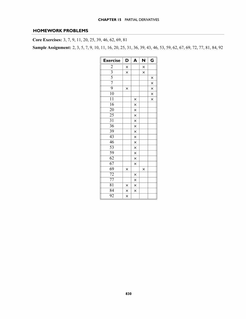
HOMEWORK PROBLEMS
Core Exercises: 3, 7, 9, 11, 20, 25, 39, 46, 62, 69, 81
Sample Assignment: 2, 3, 5, 7, 9, 10, 11, 16, 20, 25, 31, 36, 39, 43, 46, 53, 59, 62, 67, 69, 72, 77, 81, 84, 92
Exercise D A N G
2 × ×3 × ×5 ×7 ×9 × ×10 ×11 × ×16 ×20 ×25 ×31 ×36 ×39 ×43 ×46 ×53 ×59 ×62 ×67 ×69 × ×72 ×77 ×81 × ×84 × ×92 ×
830
GROUP WORK 1, SECTION 15.3
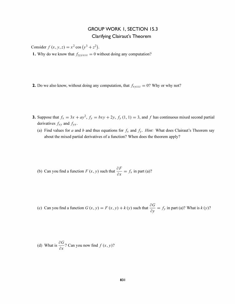
Clarifying Clairaut’s Theorem
Consider f (x, y, z) = x2 cos(y3 + z2
).
1. Why do we know that fzyyxxx = 0 without doing any computation?
2. Do we also know, without doing any computation, that fxyzzz = 0? Why or why not?
3. Suppose that fx = 3x + ay2, fy = bxy + 2y, fy (1, 1) = 3, and f has continuous mixed second partial
derivatives fxy and fyx .
(a) Find values for a and b and thus equations for fx and fy . Hint: What does Clairaut’s Theorem say
about the mixed partial derivatives of a function? When does the theorem apply?
(b) Can you find a function F (x, y) such that∂F
∂x= fx in part (a)?
(c) Can you find a function G (x, y) = F (x, y)+ k (y) such that∂G
∂y= fy in part (a)? What is k (y)?
(d) What is∂G
∂x? Can you now find f (x, y)?
831

GROUP WORK 2, SECTION 15.3
Back to the Park
The following is a map with curves of the same elevation of a region in Orangerock National Park:
We define the altitude function, A (x, y), as the altitude at a point x meters east and y meters north of the
origin (“Start”).
1. Estimate A (300, 300) and A (500, 500).
2. Estimate Ax (300, 300) and Ay (300, 300).
3. What do Ax and Ay represent in physical terms?
832

Back to the Park
4. In which direction does the altitude increase most rapidly at the point (300, 300)?
5. Use your estimates of Ax (300, 300) and Ay (300, 300) to approximate the altitude at (320, 310).
833
GROUP WORK 3, SECTION 15.3
Mixed Partials
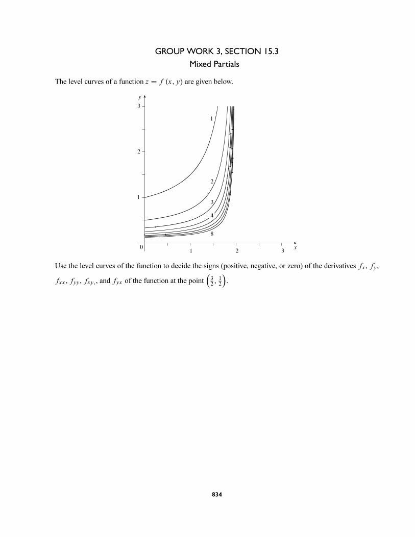
The level curves of a function z = f (x, y) are given below.
Use the level curves of the function to decide the signs (positive, negative, or zero) of the derivatives fx , fy ,
fxx , fyy , fxy,, and fyx of the function at the point(32, 12
).
834
15.4 TANGENT PLANES AND LINEAR APPROXIMATIONS
TRANSPARENCIES AVAILABLE
#43 (Figure 2), #44 (Figure 7)
SUGGESTED TIME AND EMPHASIS
1–112classes Recommended material
POINTS TO STRESS
1. The tangent plane and its analogy with the tangent line.
2. Approximation along the tangent plane and its analogy with approximation along the tangent line.
3. The meaning of differentiability in R2 and R3.
4. The difference between f being differentiable and the existence of fx and fy .
QUIZ QUESTIONS
• Text Question: Is it possible for a function f to be differentiable at (a, b) even though fx and fy do not
exist at (a, b)?
Answer: No
• Drill Question: Is it possible for a function f to be non-differentiable at (a, b) even though fx and fy
exist at (a, b)?
Answer: Yes
MATERIALS FOR LECTURE
• Discuss differentiability using both the definition and this intuitive description: f is differentiable at (a, b)
if both fx (a, b) and fy (a, b) exist and the linearization of f at (a, b) closely approximates f (x, y) when
(x, y) is sufficiently close to (a, b).
• One good example of non-differentiability is f (x, y) =⎧⎨⎩
(x − y)2
x2 + y2if (x, y) = (0, 0)
1 if (x, y) = (0, 0)
. Here
f (x, 0) ≡ 1 and f (0, y) ≡ 1, so fx and fy are both zero, but the tangent plane fails to be a good
approximation, no matter how close to the origin we look. For example, f (x, x) ≡ 0 for all x = 0.
Another good example is g (x, y) =√x2 + y2, which is continuous but not differentiable.
• Note that if the partial derivatives of a function exist and are continuous, then the tangent plane exists.
WORKSHOP/DISCUSSION
• Find an equation for the tangent plane to the top half of the unit sphere x2 + y2 + z2 = 1 at the point
(0, 0, 1) and then at(
1√2, 0, 1√
2
)using both algebraic and geometric reasoning.
• Compute some approximations to values of differentiable functions. For example, if
f (x, y) = sin(π(x2 + xy
)), then f
(12, 0)
= 1√2. Show the students how to use this fact and the
partial derivatives of f to estimate f (0.55,−0.01).
• Given f (x, y) = x2y3, find the equation for the tangent plane at (1, 1, 1), using the formula
z − z0 = fx (x0, y0) (x − x0) + fy (x0, y0) (y − y0) [Answer: z = 2 (x − 1) + 3 (y − 1) + 1.] Then
835
CHAPTER 15 PARTIAL DERIVATIVES
have the students find the tangent plane at the point (3, 1, 9). [Answer: z = 6 (x − 3)+ (y − 1)+ 9.]
This example can be extended by asking how well the tangent plane approximates the function at the given
point, perhaps by comparing f (1.1, 1.1) = 1.61 to the approximating function at (1.1, 1.1), which has
the value 1.5, and then comparing f (1.01, 1.01) ≈ 1.051 to the approximation at (1.01, 1, 01), which has
the value 1.05.
GROUP WORK 1: Trying it All Out
Problem 1 of this exercise requires the student to recognize where a complicated function is continuous.
Problem 2 can be done without a picture, but students should be encouraged to draw a picture to verify their
conclusions.
Answers:
1. (a) All points (b) All points where x = y (c) All points where x = y
2. (a) z − 2 = −32
(x − 1
3
)− (y − 2) (b) (0, 0,±3) (c) (±1, 0, 0) and (0,±3, 0)
GROUP WORK 2: Voluminous Approximations
Problem 2 may seem like “alphabet soup” to some of the students. It may be advisable to start the activity by
describing the solid in Problem 1 to the class, and then showing how 3 and 2 can be replaced by parameters,
making the volume a function of two variables r and s.
Answers:
1. 283π 2. π
3s2 (r + 2s)
3. dV = π3s2dr + 2π
3s (r + 3s) ds, so the maximum possible error is
dV = π3 (4)
(12
)+ 2π
3 (2) (3+ 6)(12
)= 20
3π ≈ 20.9
HOMEWORK PROBLEMS
Core Exercises: 1, 4, 11, 16, 20, 22, 25, 35, 41
Sample Assignment: 1, 4, 5, 7, 11, 14, 16, 17, 20, 22, 24, 25, 26, 30, 33, 35, 40, 41
Exercise D A N G
1 ×4 ×5 ×7 ×11 × ×14 × ×16 × ×17 ×20 × ×
Exercise D A N G
22 × ×24 × × ×25 ×26 ×30 ×33 × ×35 × ×40 × ×41 × ×
836
GROUP WORK 1, SECTION 15.4
Trying it All Out
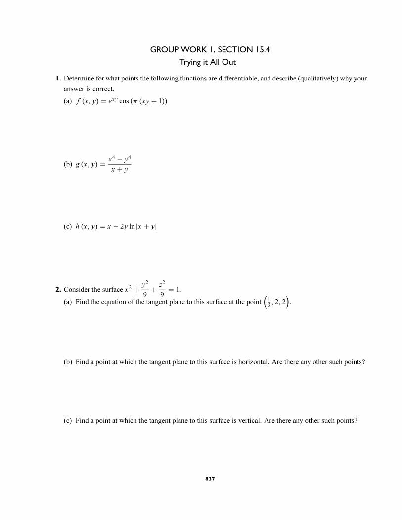
1. Determine for what points the following functions are differentiable, and describe (qualitatively) why your
answer is correct.
(a) f (x, y) = exy cos (π (xy + 1))
(b) g (x, y) = x4 − y4
x + y
(c) h (x, y) = x − 2y ln |x + y|
2. Consider the surface x2 + y2
9+ z2
9= 1.
(a) Find the equation of the tangent plane to this surface at the point(13, 2, 2
).
(b) Find a point at which the tangent plane to this surface is horizontal. Are there any other such points?
(c) Find a point at which the tangent plane to this surface is vertical. Are there any other such points?
837
GROUP WORK 2, SECTION 15.4
Voluminous Approximations
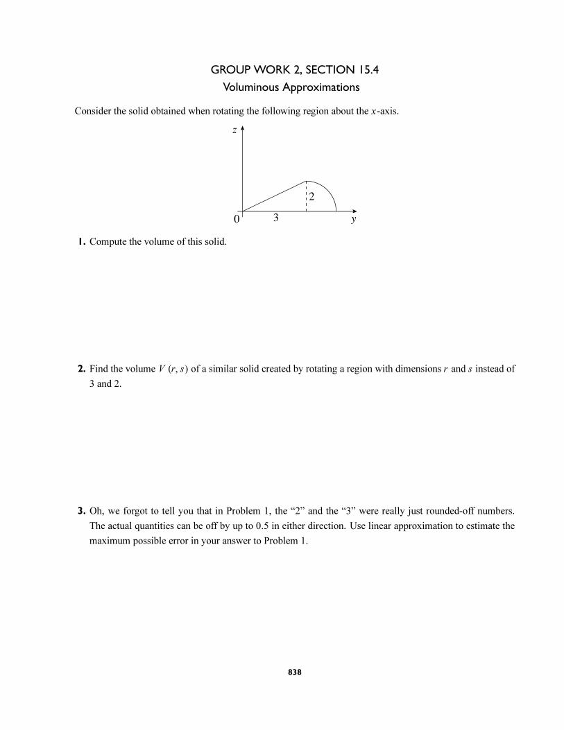
Consider the solid obtained when rotating the following region about the x-axis.
1. Compute the volume of this solid.
2. Find the volume V (r, s) of a similar solid created by rotating a region with dimensions r and s instead of
3 and 2.
3. Oh, we forgot to tell you that in Problem 1, the “2” and the “3” were really just rounded-off numbers.
The actual quantities can be off by up to 0.5 in either direction. Use linear approximation to estimate the
maximum possible error in your answer to Problem 1.
838

15.5 THE CHAIN RULE
SUGGESTED TIME AND EMPHASIS
1 class Essential material
POINTS TO STRESS
1. The extension of the Chain Rule for functions of several variables.
2. Tree diagrams.
3. Implicit differentiation.
QUIZ QUESTIONS
• Text Question: What was the following figure illustrating in the text? Specifically, how was it used?
Answer: It was used to find a Chain Rule formula for∂u
∂r,∂u
∂s, or
∂u
∂t.
• Drill Question: Suppose that f (x, y) = −x + y2, x = u2 + v3, and y = 2u − 3v . Compute ∂ f/∂u
when u = 1 and v = −1.
Answer: 18
MATERIALS FOR LECTURE
• Review the single-variable Chain Ruledy
dt= dy
dx
dx
dtusing the same language and symbols that will be
used in presenting the multivariable Chain Rule. Then develop the formulas and derivatives for chain rules
involving two and three independent variables.
• If Group Work 2: Voluminous Approximations was
covered in the previous section, extend it as follows:
Suppose that r = t + sin t and s = et − cos t vary
with time. Compute dV/dt .
839
CHAPTER 15 PARTIAL DERIVATIVES
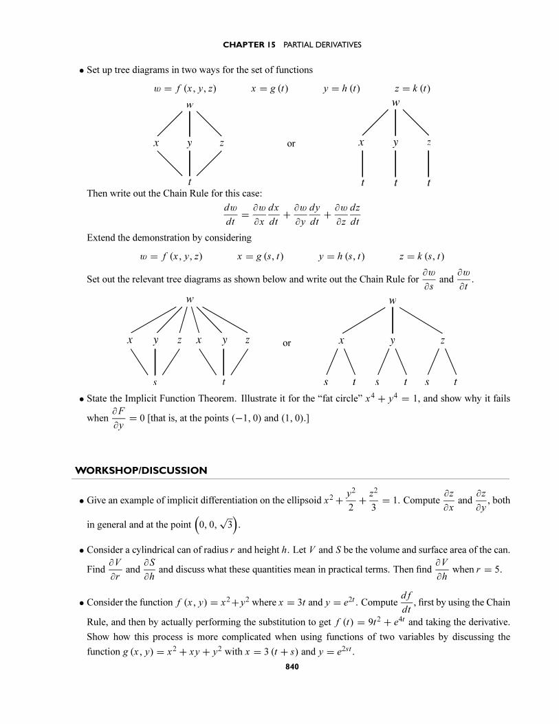
• Set up tree diagrams in two ways for the set of functions
w = f (x, y, z) x = g (t) y = h (t) z = k (t)
or
Then write out the Chain Rule for this case:
dw
dt= ∂w
∂x
dx
dt+ ∂w
∂y
dy
dt+ ∂w
∂z
dz
dt
Extend the demonstration by considering
w = f (x, y, z) x = g (s, t) y = h (s, t) z = k (s, t)
Set out the relevant tree diagrams as shown below and write out the Chain Rule for∂w
∂sand
∂w
∂t.
or
• State the Implicit Function Theorem. Illustrate it for the “fat circle” x4 + y4 = 1, and show why it fails
when∂F
∂y= 0 [that is, at the points (−1, 0) and (1, 0).]
WORKSHOP/DISCUSSION
• Give an example of implicit differentiation on the ellipsoid x2+ y2
2+ z2
3= 1. Compute
∂z
∂xand
∂z
∂y, both
in general and at the point(0, 0,
√3).
• Consider a cylindrical can of radius r and height h. Let V and S be the volume and surface area of the can.
Find∂V
∂rand
∂S
∂hand discuss what these quantities mean in practical terms. Then find
∂V
∂hwhen r = 5.
• Consider the function f (x, y) = x2+y2 where x = 3t and y = e2t . Computed f
dt, first by using the Chain
Rule, and then by actually performing the substitution to get f (t) = 9t2 + e4t and taking the derivative.
Show how this process is more complicated when using functions of two variables by discussing the
function g (x, y) = x2 + xy + y2 with x = 3 (t + s) and y = e2st .
840
SECTION 15.5 THE CHAIN RULE
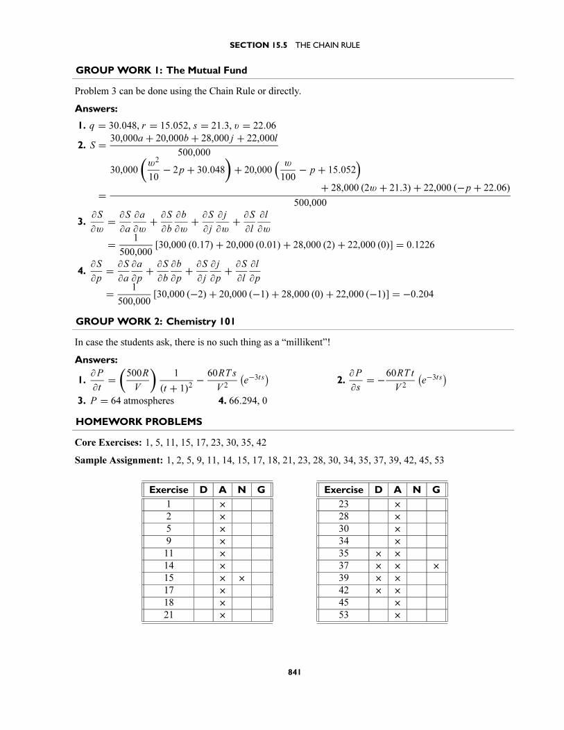
GROUP WORK 1: The Mutual Fund
Problem 3 can be done using the Chain Rule or directly.
Answers:
1. q = 30.048, r = 15.052, s = 21.3, v = 22.06
2. S = 30,000a + 20,000b + 28,000 j + 22,000l
500,000
=
30,000
(w2
10− 2p + 30.048
)+ 20,000
( w
100− p + 15.052
)+ 28,000 (2w + 21.3)+ 22,000 (−p + 22.06)
500,000
3.∂S
∂w= ∂S
∂a
∂a
∂w+ ∂S
∂b
∂b
∂w+ ∂S
∂ j
∂ j
∂w+ ∂S
∂l
∂l
∂w
= 1
500,000[30,000 (0.17)+ 20,000 (0.01)+ 28,000 (2)+ 22,000 (0)] = 0.1226
4.∂S
∂p= ∂S
∂a
∂a
∂p+ ∂S
∂b
∂b
∂p+ ∂S
∂ j
∂ j
∂p+ ∂S
∂l
∂l
∂p
= 1
500,000[30,000 (−2)+ 20,000 (−1)+ 28,000 (0)+ 22,000 (−1)] = −0.204
GROUP WORK 2: Chemistry 101
In case the students ask, there is no such thing as a “millikent”!
Answers:
1.∂P
∂t=(500R
V
)1
(t + 1)2− 60RT s
V 2
(e−3ts
)2.
∂P
∂s= −60RT t
V 2
(e−3ts
)3. P = 64 atmospheres 4. 66.294, 0
HOMEWORK PROBLEMS
Core Exercises: 1, 5, 11, 15, 17, 23, 30, 35, 42
Sample Assignment: 1, 2, 5, 9, 11, 14, 15, 17, 18, 21, 23, 28, 30, 34, 35, 37, 39, 42, 45, 53
Exercise D A N G
1 ×2 ×5 ×9 ×11 ×14 ×15 × ×17 ×18 ×21 ×
Exercise D A N G
23 ×28 ×30 ×34 ×35 × ×37 × × ×39 × ×42 × ×45 ×53 ×
841

GROUP WORK 1, SECTION 15.5
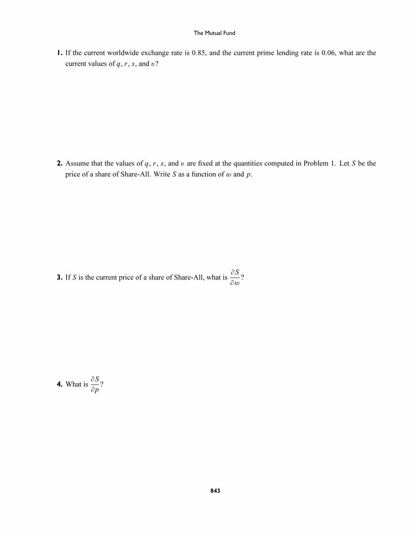
The Mutual Fund
One of the hottest investments on Wall Street today is the Share-All Mutual Fund. The Share-All Fund has
issued 500,000 shares for eager investors to buy. Each share, therefore, represents 1500,000
of the fund’s total
net asset value. The fund owns 100,000 shares of stock in four companies, as described below, on a given day.
Company Name Current price/shareNumber of Shares
Owned by Share-AllTotal $ value
Allied Oil 30 30,000 900,000
Beck Keyboard Manufacturing 15 20,000 300,000
Jasmine Tea 23 28,000 644,000
Lapland Importing-Exporting 22 22,000 484,000
Total asset value 2,328,000
So, on this day, the total asset value is $2,328,000, and the price of one share of Share-All is
2,328,000
500,000= $4.656.
Many factors affect the price of a stock. For example, the worldwide exchange rate* w affects the Lapland
Importing-Exporting company much more than it does the primarily domestic Beck Keyboard Manufacturing
company. Similarly, the United States prime lending rate p affects the highly indebted Allied Oil company
more than it affects the relatively debt-free Jasmine Tea company. Thus, we can develop models for the price
of these stocks as functions of the world-wide exchange rate, the prime lending rate, and other economic
factors q, r , s, and v , which are independent of these variables.
Let w be the world-wide exchange rate, and p be the U.S. prime lending rate. Let a (w, p, q), b (w, p, r),
j (w, p, s), and l (w, p, v) be the current price per share of Allied, Beck, Jasmine and Lapland respectively.
We have
a (w, p, q) = 0.1w2 − 2p + q
b (w, p, r) = 0.01w − p + r
j (w, p, s) = 2w + s
l (w, p, v) = −p + v
where q, r , s and v are composite variables representing the myriad other factors that affect the price of these
stocks, and are independent of w and p. (Note: If we knew q, r , s, and v exactly, then we would be able to
predict the price of the stock with unrealistic accuracy.)
* The worldwide exchange rate measures the value of the dollar measured versus a weighted average of other relevant
currencies. In other words, it is a statistic which we made up, but which could probably fool some people.
842
The Mutual Fund
1. If the current worldwide exchange rate is 0.85, and the current prime lending rate is 0.06, what are the
current values of q, r , s, and v?
2. Assume that the values of q, r , s, and v are fixed at the quantities computed in Problem 1. Let S be the
price of a share of Share-All. Write S as a function of w and p.
3. If S is the current price of a share of Share-All, what is∂S
∂w?
4. What is∂S
∂p?
843
GROUP WORK 2, SECTION 15.5
Chemistry 101
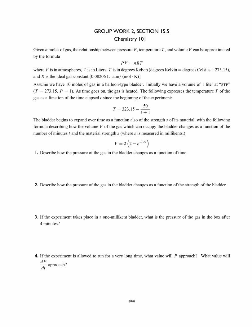
Given n moles of gas, the relationship between pressure P , temperature T , and volume V can be approximated
by the formula
PV = nRT
where P is in atmospheres, V is in Liters, T is in degrees Kelvin (degrees Kelvin= degrees Celsius+273.15),
and R is the ideal gas constant [0.08206 L · atm/ (mol · K)]Assume we have 10 moles of gas in a balloon-type bladder. Initially we have a volume of 1 liter at “STP”
(T = 273.15, P = 1). As time goes on, the gas is heated. The following expresses the temperature T of the
gas as a function of the time elapsed t since the beginning of the experiment:
T = 323.15− 50
t + 1
The bladder begins to expand over time as a function also of the strength s of its material, with the following
formula describing how the volume V of the gas which can occupy the bladder changes as a function of the
number of minutes t and the material strength s (where s is measured in millikents.)
V = 2(2− e−3ts
)1. Describe how the pressure of the gas in the bladder changes as a function of time.
2. Describe how the pressure of the gas in the bladder changes as a function of the strength of the bladder.
3. If the experiment takes place in a one-millikent bladder, what is the pressure of the gas in the box after
4 minutes?
4. If the experiment is allowed to run for a very long time, what value will P approach? What value will
dP
dtapproach?
844
15.6 DIRECTIONAL DERIVATIVES AND THE GRADIENT VECTOR
TRANSPARENCY AVAILABLE
#45 (Figures 3 and 5)
SUGGESTED TIME AND EMPHASIS
1–112classes Essential material
POINTS TO STRESS
1. The computation and geometric meaning of a directional derivative.
2. The computation of a gradient vector.
3. The geometric meanings of a gradient vector: A normal vector to a surface, the direction of greatest
change, a perpendicular vector to contour curves and surfaces, a vector with length equal to the maximum
value of the directional derivative.
4. The relationships between tangent planes, gradient vectors, and directional derivatives.
QUIZ QUESTIONS
• Text Question: The text shows that Du f (x, y) = ∇ f (x, y) · u, where u is a unit vector Why does this
express the directional derivative in the direction of u as the scalar projection of the gradient vector onto
u?
Answer: This follows directly from the scalar projection formula.
• Drill Question: If f (x, y) = xy2 + x , what is∇ f (x, y)?
Answer:⟨y2 + 1, 2xy
⟩MATERIALS FOR LECTURE
• Show how the gradient, while relatively simple to compute, yields a treasure trove of useful information.
• Define S to be a level surface of the function f (x, y, z). Explain why∇ f (x0, y0, z0) is orthogonal to the
surface at any point P (x0, y0, z0) on S. Define the tangent plane to S at P to be the plane with normal
vector ∇ f (x0, y0, z0).
• Review that the direction of any vector v = 0 is determined by the unit vector u = v
|v| = 〈cosθ, sinθ〉where θ is the angle that v makes with the positive x-axis. Using this interpretation, the directional
derivative formula can be rewritten as
Du f = ∂ f
∂xcosθ + ∂ f
∂ysinθ
• Let f (x, y) = x2y2. Compute Du f (x, y) for unit vectors u making angles of 0, π6, π4, π3, and π
2with the
positive x-axis, and fill in the following table. Point out that the coefficient of 2xy2 decreases from 1 to 0
while the coefficient of 2x2y increases from 0 to 1. Have the students reason intuitively why this should be
the case, just using the concept of “directional derivative”. Have them figure out (intuitively) Du f (x, y)
845
CHAPTER 15 PARTIAL DERIVATIVES
for angles π and 3π2.
Angle Du f (x, y)
0 (1) 2xy2 + (0) 2x2y
π6
(0.866 . . .) 2xy2 + (0.5) 2x2y
π4
(0.707 . . .) 2xy2 + (0.707 . . .) 2x2y
π3
(0.5) 2xy2 + (0.866...) 2x2y
π2
(0) 2xy2 + (1) 2x2y
Note: At a given point (x, y), one cannot maximize Du merely by looking at the chart.
• Show how Equation 2 in the Section 15.4 is really just a special case of Equation 19 in this section.
WORKSHOP/DISCUSSION
• Consider the surface f (x, y) = xy at the point (0, 0) . Note that although the maximum rate of change
is zero at that point, it is not the case that the function is identically zero near the origin. Thus, if
∇ f (a, b) = 0, we cannot talk about the direction of maximal change at (a, b).
• Have the students practice finding the directional derivatives of f = x2y and f = exy in the directions
−i, i + j, −i − j, and i − j. Also have them find the directional derivatives of f (x, y, z) = z2exy2
in the
directions of 〈−1,−1,−1〉 and 〈0, 0,−1〉.• Show that the gradient vector ∇ f (x0, y0) is normal to the line tangent to the level curve k = f (x, y)
at the point (x0, y0). Look at the example f (x, y) = 5x4 + 4xy + 3y2 and show that
∇ f (−1,−1) = 〈−24,−10〉. Conclude that we now know that f is decreasing in both the x- and y-
directions and that the direction of maximal increase is 〈−24,−10〉. Ask the students to resolve these
seemingly contradictory observations: That the gradient is supposed to point in the direction of maximal
increase, yet the components fx (−1,−1) = −24 and fy (−1,−1) = −10 of the gradient are pointing in
the direction of decreasing x and y. (Although no real paradox exists, students are often confused by this
type of situation.)
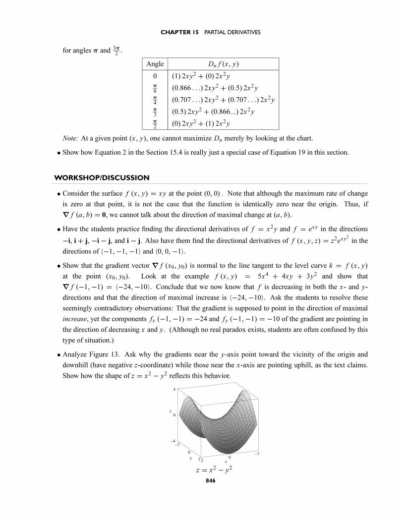
• Analyze Figure 13. Ask why the gradients near the y-axis point toward the vicinity of the origin and
downhill (have negative z-coordinate) while those near the x-axis are pointing uphill, as the text claims.
Show how the shape of z = x2 − y2 reflects this behavior.
z = x2 − y2
846
SECTION 15.6 DIRECTIONAL DERIVATIVES AND THE GRADIENT VECTOR
GROUP WORK 1: Two Ways
This exercise ties together many of the key concepts from this section. Therefore, closure is particularly
important here.
Answers:
1. 5 2. 7√2 3. 6 cosθ + 8 sinθ
4. 10 (They should find this by optimizing the single-variable function f (θ) = 6 cosθ + 8 sinθ.)
5. θ = 0.9273 radians 6. 〈0.6, 0.8〉 7. 10, 〈0.6, 0.8〉GROUP WORK 2: Computation Practice
It is a good idea to give the students a chance for guided practice using the types of computations that will
be required on the homework. We recommend having them do either Problem 1 or Problem 2 in groups, and
then handing the remaining problem out as a worksheet.
Answers:
1. (a) e − 2 (b) e (c)√2 (e − 1) (d) − ln 2√
3(e) − ln 2√
6
2. (a) Maximum: 〈e − 2, e〉, minimum: 〈2− e,−e〉 (b) Maximum: 〈0, 0, ln 2〉, minimum: 〈0, 0,− ln 2〉GROUP WORK 3: Bowling Balls and Russian Weebles
This exercise may seem trivial, but it is a good setup for discussions of Lagrange multipliers. If the students
do this exercise, ask them to remember the result, and make sure to remind them of the bowling balls and
Russian weebles when discussing Lagrange multipliers.
Answers:
1. Parallel, opposite directions. Same tangent plane. No difference.
2. Parallel, same direction. Same tangent plane 3. Parallel, same tangent plane
HOMEWORK PROBLEMS
Core Exercises: 1, 6, 8, 11, 23, 30, 36
Sample Assignment: 1, 5, 6, 8, 11, 12, 15, 19, 23, 25, 28, 30, 34, 36, 38, 40, 43, 47, 52, 62
Exercise D A N G
1 × ×5 ×6 ×8 ×11 ×12 ×15 ×19 ×23 ×25 ×
Exercise D A N G
28 ×30 × ×34 × ×36 ×38 × ×40 ×43 ×47 × ×52 ×62 × × ×
847
GROUP WORK 1, SECTION 15.6
Two Ways
Consider the function f (x, y) = x2 + 4xy2.
1. What is f (1, 1)?
2. What is the directional derivative Du (1, 1) if u =⟨
1√2, 1√
2
⟩?
3. What is the directional derivative Du (1, 1) if u is the unit vector that makes an angle θ with the positive
x-axis?
4. In Problem 3, you expressed Du (1, 1) as a function of the angle θ. Let’s say we want to find the maximum
value of the directional derivative. This is now a single-variable calculus problem! Use your single-
variable calculus techniques, coupled with your answer to Problem 3, to find the find the maximum value
of the directional derivative.
5. What is the angle θ for which f increases the fastest? (You should be able to use your computations for
Problem 4 to answer this one quickly.)
6. What is the unit vector that makes that angle θ with the positive x-axis?
7. Now compute |∇ f | and ∇ f
|∇ f | , but before you do so, discuss with your group members what the answers
should be. You should be able to anticipate the correct answers.
848
GROUP WORK 2, SECTION 15.6
Computation Practice
1. Find the directional derivative of the function at the given point in the direction of the given vector v.
(a) f (x, y) = exy − x2, (1, 1), v = 〈1, 0〉
(b) f (x, y) = exy − x2, (1, 1), v = 〈0, 1〉
(c) f (x, y) = exy − x2, (1, 1), v = 〈1, 1〉
(d) f (x, y, z) = z ln(x2 + y2
), (−1, 1, 0), v = 〈1, 1,−1〉
(e) f (x, y, z) = z ln(x2 + y2
), (−1, 1, 0), v = 〈2, 1, 1〉
849
Computation Practice
2. Find the maximum and minimum rates of change of f at the given point and the directions in which they
occur.
(a) f (x, y) = exy − x2, (1, 1)
(b) f (x, y, z) = z ln(x2 + y2
), (−1, 1, 0)
850
GROUP WORK 3, SECTION 15.6
Bowling Balls and Russian Weebles
1. Assume that there are two bowling balls in a ball-return machine. They are touching each other. At the
point at which they touch, what can you say about their respective normal vectors? What about their
tangent planes? What would happen if the bowling balls were of different sizes?
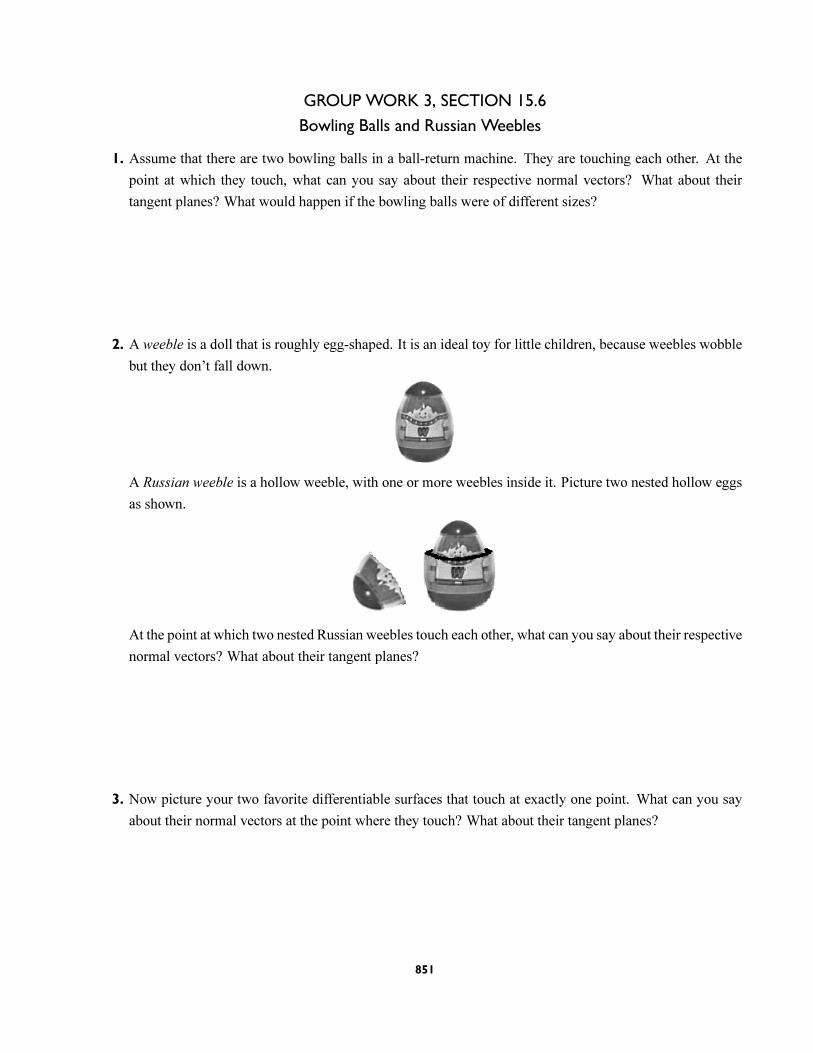
2. A weeble is a doll that is roughly egg-shaped. It is an ideal toy for little children, because weebles wobble
but they don’t fall down.
A Russian weeble is a hollow weeble, with one or more weebles inside it. Picture two nested hollow eggs
as shown.
At the point at which two nested Russian weebles touch each other, what can you say about their respective
normal vectors? What about their tangent planes?
3. Now picture your two favorite differentiable surfaces that touch at exactly one point. What can you say
about their normal vectors at the point where they touch? What about their tangent planes?
851
15.7 MAXIMUM AND MINIMUM VALUES
TRANSPARENCY AVAILABLE
#46 (Figures 7–9)
SUGGESTED TIME AND EMPHASIS
1 class Essential material
POINTS TO STRESS
1. The contrast between optimization problems in single-variable calculus (relatively few cases) and in
multivariable calculus (many possible solutions)
2. Critical points and local maxima and minima
3. The Second Derivative Test.
4. Absolute maxima and minima
QUIZ QUESTIONS
• Text Question: Can a differentiable function f have a local maximum at a point (a, b) with fx (a, b) =3?
Answer: No
• Drill Question: Can you give an example of a function f with the property that fx (a, b) = 0,
fy (a, b) = 0, and f does not have a local maximum or minimum at (a, b)?
Answer: f (x, y) = xy at (0, 0).
MATERIALS FOR LECTURE
A good way to introduce this topic may be to have the students do Group Work 1: Foreshadowing Critical
Points and Extrema.
• Stress geometric interpretations: If f is differentiable at a local maximum or minimum, then the tangent
plane must be horizontal. Note that there are critical points at which there is no local maximum or
minimum. For example, examine the saddle points at the origin for f (x, y) = xy and g (x, y) = x2 − y2.
852
SECTION 15.7 MAXIMUM AND MINIMUM VALUES
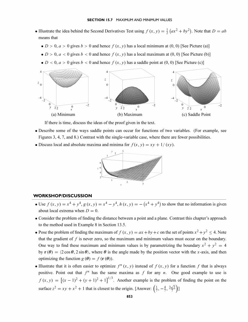
• Illustrate the idea behind the Second Derivatives Test using f (x, y) = 12
(ax2 + by2
). Note that D = ab
means that
• D > 0, a > 0 gives b > 0 and hence f (x, y) has a local minimum at (0, 0) [See Picture (a)]
• D > 0, a < 0 gives b < 0 and hence f (x, y) has a local maximum at (0, 0) [See Picture (b)]
• D < 0, a > 0 gives b < 0 and hence f (x, y) has a saddle point at (0, 0) [See Picture (c)]
(a) Minimum (b) Maximum (c) Saddle Point
If there is time, discuss the ideas of the proof given in the text.
• Describe some of the ways saddle points can occur for functions of two variables. (For example, see
Figures 3, 4, 7, and 8.) Contrast with the single-variable case, where there are fewer possibilities.
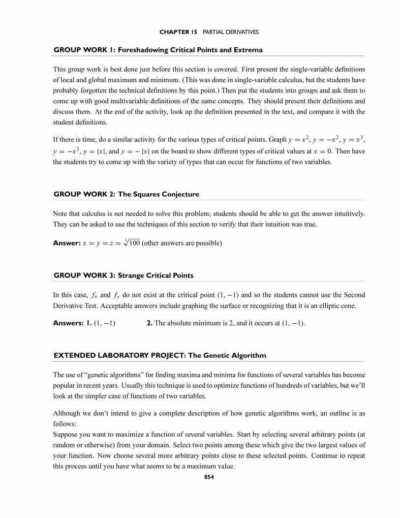
• Discuss local and absolute maxima and minima for f (x, y) = xy + 1/ (xy).
WORKSHOP/DISCUSSION
• Use f (x, y) = x4 + y4, g (x, y) = x4 − y4, h (x, y) = − (x4 + y4)to show that no information is given
about local extrema when D = 0.
• Consider the problem of finding the distance between a point and a plane. Contrast this chapter’s approach
to the method used in Example 8 in Section 13.5.
• Pose the problem of finding the maximum of f (x, y) = ax+by+c on the set of points x2+ y2 ≤ 4. Note
that the gradient of f is never zero, so the maximum and minimum values must occur on the boundary.
One way to find these maximum and minimum values is by parametrizing the boundary x2 + y2 = 4
by r (θ) = 〈2 cosθ, 2 sinθ〉, where θ is the angle made by the position vector with the x-axis, and then
optimizing the function g (θ) = f (r (θ)).
• Illustrate that it is often easier to optimize f n (x, y) instead of f (x, y) for a function f that is always
positive. Point out that f n has the same maxima as f for any n. One good example to use is
f (x, y) = [(x − 1)2 + (y + 1)2 + 1
]1/3. Another example is the problem of finding the point on the
surface z2 = xy + x2 + 1 that is closest to the origin. [Answer:(17,−4
7, 3
√2
7
)]
853
CHAPTER 15 PARTIAL DERIVATIVES
GROUP WORK 1: Foreshadowing Critical Points and Extrema
This group work is best done just before this section is covered. First present the single-variable definitions
of local and global maximum and minimum. (This was done in single-variable calculus, but the students have
probably forgotten the technical definitions by this point.) Then put the students into groups and ask them to
come up with good multivariable definitions of the same concepts. They should present their definitions and
discuss them. At the end of the activity, look up the definition presented in the text, and compare it with the
student definitions.
If there is time, do a similar activity for the various types of critical points. Graph y = x2, y = −x2, y = x3,
y = −x3, y = |x |, and y = − |x| on the board to show different types of critical values at x = 0. Then have
the students try to come up with the variety of types that can occur for functions of two variables.
GROUP WORK 2: The Squares Conjecture
Note that calculus is not needed to solve this problem; students should be able to get the answer intuitively.
They can be asked to use the techniques of this section to verify that their intuition was true.
Answer: x = y = z = 3√100 (other answers are possible)
GROUP WORK 3: Strange Critical Points
In this case, fx and fy do not exist at the critical point (1,−1) and so the students cannot use the Second
Derivative Test. Acceptable answers include graphing the surface or recognizing that it is an elliptic cone.
Answers: 1. (1,−1) 2. The absolute minimum is 2, and it occurs at (1,−1).
EXTENDED LABORATORY PROJECT: The Genetic Algorithm
The use of “genetic algorithms” for finding maxima and minima for functions of several variables has become
popular in recent years. Usually this technique is used to optimize functions of hundreds of variables, but we’ll
look at the simpler case of functions of two variables.
Although we don’t intend to give a complete description of how genetic algorithms work, an outline is as
follows:
Suppose you want to maximize a function of several variables. Start by selecting several arbitrary points (at
random or otherwise) from your domain. Select two points among these which give the two largest values of
your function. Now choose several more arbitrary points close to these selected points. Continue to repeat
this process until you have what seems to be a maximum value.
854
SECTION 15.7 MAXIMUM AND MINIMUM VALUES
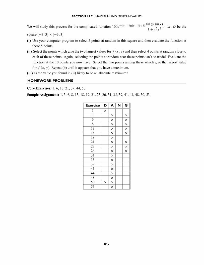
We will study this process for the complicated function 100e−(|x| + 1)(|y+ 1| + 1) sin (y sin x)
1+ x2y2. Let D be the
square [−3, 3]× [−3, 3].
(i) Use your computer program to select 5 points at random in this square and then evaluate the function at
these 5 points.
(ii) Select the points which give the two largest values for f (x, y) and then select 4 points at random close to
each of these points. Again, selecting the points at random near these points isn’t so trivial. Evaluate the
function at the 10 points you now have. Select the two points among these which give the largest value
for f (x, y). Repeat (b) until it appears that you have a maximum.
(iii) Is the value you found in (ii) likely to be an absolute maximum?
HOMEWORK PROBLEMS
Core Exercises: 3, 6, 13, 21, 39, 44, 50
Sample Assignment: 1, 3, 6, 8, 13, 18, 19, 21, 23, 26, 31, 35, 39, 41, 44, 48, 50, 53
Exercise D A N G
1 ×3 × ×6 × ×8 × ×13 × ×18 × ×19 ×21 × ×23 × ×26 × ×31 ×35 ×39 ×41 ×44 ×48 ×50 × ×53 ×
855
GROUP WORK 2, SECTION 15.7
The Squares Conjecture
You are given a government grant to prove or disprove the Squares Conjecture:
There exist three positive numbers, r , s, t whose product is 100, yet
have the property that the sum of their squares is less than 65.
Either find three such numbers, or show that none exist.
856
GROUP WORK 3, SECTION 15.7
Strange Critical Points
Let f (x, y) = 2+√3 (x − 1)2 + 4 (y + 1)2.
1. Find the critical points of f .
2. Find the local and absolute minimum values of f . Where do these values occur?
857
APPLIED PROJECT Designing a Dumpster
This project requires the students to solve an extended real-world problem that involves them going out and
measuring a nearby dumpster. They will have to make approximations, and figure out how best to get an
accurate answer. A good sample answer is given in the Complete Solutions Manual.
The project can be made more applied if the students are instructed to actually research the costs involved,
instead of using the ones provided in the problem statement.
DISCOVERY PROJECT Quadratic Approximations and Critical Points
Problems 1–3 serve as a good introduction to Taylor’s Theorem for two variables, and to quadratic polynomial
approximation in two variables. Problems 4 and 5 justify the Second Derivative Test, the proof of which is
given in Appendix F.
858
15.8 LAGRANGE MULTIPLIERS
TRANSPARENCY AVAILABLE
#47 (Figures 2 and 3)
SUGGESTED TIME AND EMPHASIS
1 class Essential material
POINTS TO STRESS
1. The geometric justification for the method of Lagrange multipliers
2. How to apply the method of Lagrange multipliers, including the extension of the method for two-constraint
problems
QUIZ QUESTIONS
• Text Question: How does the equation∇ f (x, y) = λ∇g (x, y), subject to the constraint g (x, y) = k,
lead to three equations with three unknowns? What are the unknowns?
Answer: The constraint gives one equation, and the gradient (consisting of two dimensions) gives the
other two. x , y, and λ are the unknowns.
MATERIALS FOR LECTURE
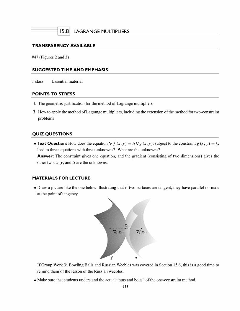
• Draw a picture like the one below illustrating that if two surfaces are tangent, they have parallel normals
at the point of tangency.
If Group Work 3: Bowling Balls and Russian Weebles was covered in Section 15.6, this is a good time to
remind them of the lesson of the Russian weebles.
• Make sure that students understand the actual “nuts and bolts” of the one-constraint method.
859
CHAPTER 15 PARTIAL DERIVATIVES
• Give an example to show that, with functions of two variables, there are often alternate methods other than
Lagrange multipliers to solve optimization problems. Perhaps redo Example 2, substituting x2 = 1 − y2
into f (x, y) = x2 + 2y2 to get the single-variable problem g (y) = 1+ y2, minimize to get y = 0 (with
x = ±1), and then get h (x) = 2 − x2 with maximum x = 0, y = ±1. Perhaps also note that, for the
two-variable case, ∇ f = λ∇g implies that ∇ f × ∇g = 0. This condition can sometimes be used to
replace Lagrange multipliers.
WORKSHOP/DISCUSSION
• Find the volume of the largest rectangular solid that can be inscribed in a sphere, that is, maximize
V (x, y, z) = (2x) (2y) (2z) given that x2 + y2 + z2 = a2.
• Discuss the geometric solution to Example 4. What basic geometric principle is being used?
GROUP WORK 1: The Inscribed Rectangle Race
Divide the class in half. Write the following problem on the board: “What is the area of the largest rectangle
that can be inscribed in a circle of radius 4?” Have one half of the class try to solve this problem using
Lagrange multipliers, and the other half try to use single-variable calculus. See which side finishes first, and
which side found the problem more difficult. At the end, the students should see both methods presented.
If a group finishes early, or after all groups have presented, have the students further practice the two tech-
niques by maximizing xy2 on the ellipse 19x2 + 1
4y2 = 1.
Answers: 4, 8√3
3
GROUP WORK 2: Biggest and Smallest on Closed and Bounded Sets
This activity involves finding the absolute maximum and minimum values of a function of several variables
on a closed and bounded set. Review the necessary steps outlined in Section 15.7.
Answers: 2, −1
GROUP WORK 3: The Heated Cannonball
This problem appears to be quite difficult at first reading, but letting x , y, and z be the angles (in radians) and
using Lagrange multipliers leads to a very easy solution.
Answers:
1. The minimum is −60◦ at the points (±1, 0, 0). The maximum is 60◦ wherever y2 + z2 = 1.
2. It is a circular frame in the yz-plane.
860
SECTION 15.8 LAGRANGE MULTIPLIERS
GROUP WORK 4: The Sum of the Sines
Answers: 1. Equilateral 2. 3√3
23. 45◦-45◦-90◦, 1+√
2
HOMEWORK PROBLEMS
Core Exercises: 1, 3, 10, 18, 20, 25, 36
Sample Assignment: 1, 3, 6, 10, 11, 18, 20, 25, 27, 32, 36, 38, 43
Exercise D A N G
1 × ×3 ×6 ×10 ×11 ×18 ×20 × × ×25 ×27 ×32 ×36 ×38 ×43 × ×
861
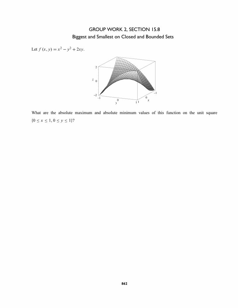
GROUP WORK 2, SECTION 15.8
Biggest and Smallest on Closed and Bounded Sets
Let f (x, y) = x2 − y2 + 2xy.
What are the absolute maximum and absolute minimum values of this function on the unit square
{0 ≤ x ≤ 1, 0 ≤ y ≤ 1}?
862
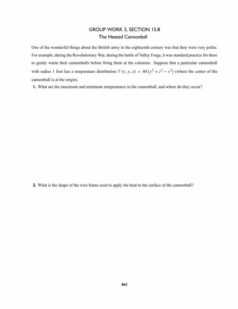
GROUP WORK 3, SECTION 15.8
The Heated Cannonball
One of the wonderful things about the British army in the eighteenth century was that they were very polite.
For example, during the RevolutionaryWar, during the battle of Valley Forge, it was standard practice for them
to gently warm their cannonballs before firing them at the colonists. Suppose that a particular cannonball
with radius 1 foot has a temperature distribution T (x, y, z) = 60(y2 + z2 − x2
)(where the center of the
cannonball is at the origin).
1. What are the maximum and minimum temperatures in the cannonball, and where do they occur?
2. What is the shape of the wire frame used to apply the heat to the surface of the cannonball?
863
GROUP WORK 4, SECTION 15.8
The Sum of the Sines
1. What is the description of the triangle for which the sum of the sines of its angles is a maximum?
2. Find the maximal value of the sums of the sines of the angles of a triangle.
3. Repeat Problems 1 and 2 if we now assume that the triangle is a right triangle.
864
APPLIED PROJECT Rocket Science
This is an excellent example of Lagrange multipliers presented in a realistic setting. If not assigned as a
project, it can be given as a supplementary reading. The computations required for this problem are extensive.
A CAS might help, but is not required.
APPLIED PROJECT Hydro-Turbine Optimization
This problem has not been simplified. The Great Northern Paper Company is a real company that has hired
people to solve the same problem that the students are faced with. If this project is assigned, the students
should be informed that they have the opportunity to solve a real engineering problem. You can specify that
the final report be written up in a professional manner so that the students can show the report to prospective
employers.
865
15 SAMPLE EXAM
Problems marked with an asterisk (*) are particularly challenging and should be given careful consideration.
1. (a) Consider the function f (x, y) = 1
x2 + y2 + 1. Find equations for the following level surfaces for f ,
and sketch them.
(i) f (x, y) = 15
(ii) f (x, y) = 110
(b) Find k such that the level surface f (x, y) = k consists of a single point.
(c) Why is k the global maximum of f (x, y)?
2. Is the function f (x, y) = sin2(xy2)a solution to the partial differential equation
∂ f
∂x+ ∂ f
∂y= (2x + y) (2y) cos
(xy2)√
f when sin(xy2) ≥ 0?
3. Is it possible to find a function for which it is true that, for all x > 0 and y > 0, fx > 0 and fy < 0, and
f (x, y) > 0? If so, give an example. If not, why not?
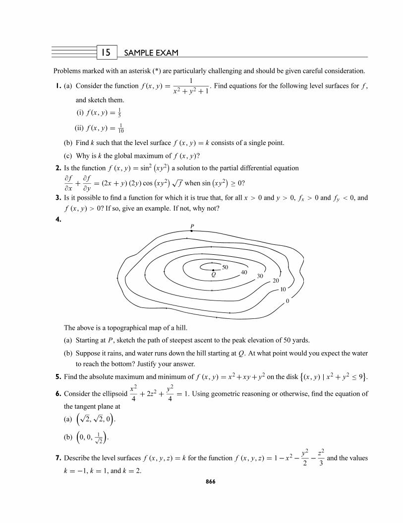
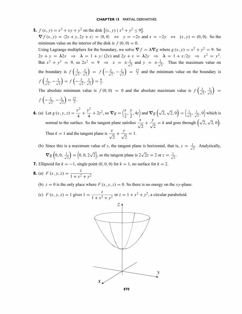
4.
The above is a topographical map of a hill.
(a) Starting at P , sketch the path of steepest ascent to the peak elevation of 50 yards.
(b) Suppose it rains, and water runs down the hill starting at Q. At what point would you expect the water
to reach the bottom? Justify your answer.
5. Find the absolute maximum and minimum of f (x, y) = x2+ xy+ y2 on the disk{(x, y) | x2 + y2 ≤ 9
}.
6. Consider the ellipsoidx2
4+ 2z2 + y2
4= 1. Using geometric reasoning or otherwise, find the equation of
the tangent plane at
(a)(√
2,√2, 0).
(b)(0, 0, 1√
2
).
7. Describe the level surfaces f (x, y, z) = k for the function f (x, y, z) = 1− x2− y2
2− z2
3and the values
k = −1, k = 1, and k = 2.
866
CHAPTER 15 SAMPLE EXAM
8. Suppose that the amount of energy F (x, y, z) emanating from a source at (0, 0, 0) is inversely
proportional to one more than the square of the distance from the origin measured only in the the xy-
plane, and is directly proportional to the height above the xy-plane. Assume that all of the constants of
proportionality are equal to 1.
(a) What is an equation for the energy as a function of x , y, and z?
(b) Where is there no energy at all?
(c) Sketch the level surface F (x, y, z) = 1.
9. Consider the function
f (x, y) = x + y
|x| + |y|(a) Evaluate the following
(i) f (1, 1)
(ii) f (1,−1)
(iii) f (−1, 1)
(iv) f (−1,−1)
(b) Does this function have a limit at (0, 0)?
10. Consider the function
f (x, y) =⎧⎨⎩
2x2 + 3y2
x − yif x = y
0 if x = y
(a) Compute fx (0, 0) directly from the limit definition of a partial derivative
fx (x0, y0) = limh→0
f (x0 + h, y0)− f (x0, y0)
h
(b) Compute fy (0, 0).
11. If f (0, 0) = 0, fx (0, 0) = 0, fy (0, 0) = 0, and f (x, y) is differentiable at (0, 0), does this imply that
f (x, y) = 0 for some point (x, y) = (0, 0)? Justify your result, or give a counterexample.
12. Consider the sphere x2 + y2 + z2 = 9. Find the equation of the plane tangent to this sphere at
(a) (3, 0, 0).
(b) (2, 2, 1).
13. Suppose that f (x, y) = ex − y and f (ln 2, ln 2) = 1. Use the technique of linear approximation to
estimate f (ln 2+ 0.1, ln 2+ 0.04).
14. Let g (u) be a differentiable function and let f (x, y) = g(x2 + y2
).
(a) Show that y fx = x fy .
(b) Find the direction of maximal increase of f at (1, 1) in terms of g′.867
CHAPTER 15 PARTIAL DERIVATIVES
15. Let f be a function of two variables with the following properties:
• ∂ f
∂xis defined near (0, 0), continuous at (0, 0) and
∂ f
∂x(0, 0) = 0
• ∂ f
∂yis defined near (0, 0), continuous at (0, 0) and
∂ f
∂y(0, 0) = 0
• ∂2 f
∂x∂y(0, 0) = 1
• ∂2 f
∂y∂x(0, 0) = −1
Answer true or false to the following, and give reasons for your answers.
(a) f is differentiable at (0, 0).
(b) There is a horizontal plane that is tangent to the graph of f at (0, 0).
(c) The functions∂2 f
∂x∂yand
∂2 f
∂y∂xare both continuous at (0, 0).
(d) The linear approximation to f (x, y) at (0, 0) is L (x, y) = x − y.
16. Suppose u = 〈1, 0〉, v =⟨
1√2, 1√
2
⟩, Du ( f (a, b)) = 3 and Dv ( f (a, b)) =
√2.
(a) Find∇ f (a, b).
(b) What is the maximum possible value of Dw ( f (a, b)) for any w?
(c) Find a unit vector w = 〈w1, w2〉 such that Dw ( f (a, b)) = 0.
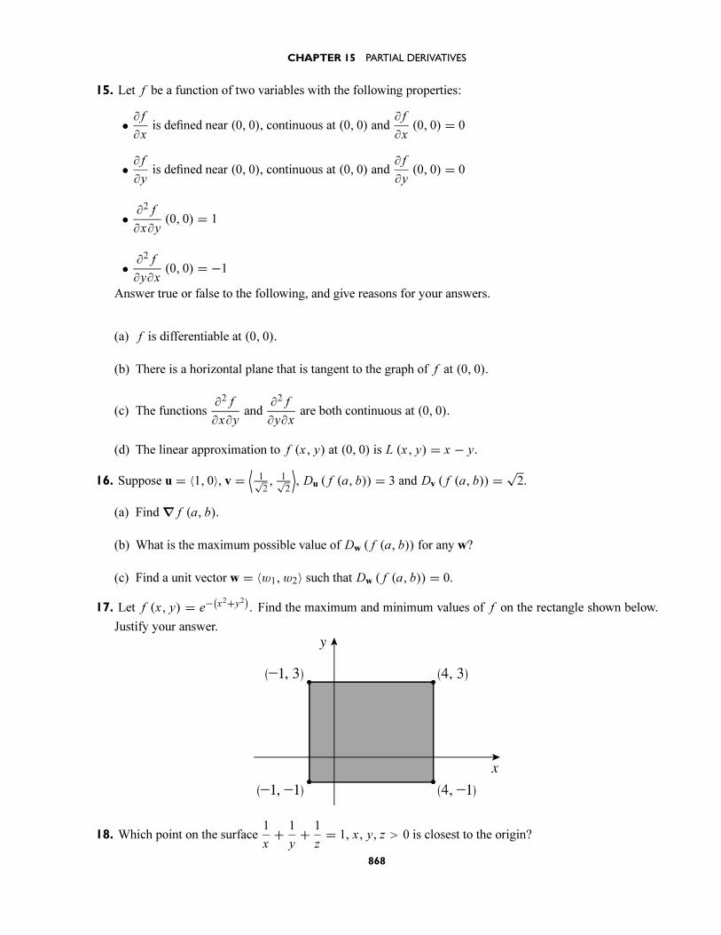
17. Let f (x, y) = e−(x2+y2
). Find the maximum and minimum values of f on the rectangle shown below.
Justify your answer.
18. Which point on the surface1
x+ 1
y+ 1
z= 1, x , y, z > 0 is closest to the origin?
868
15 SAMPLE EXAM SOLUTIONS
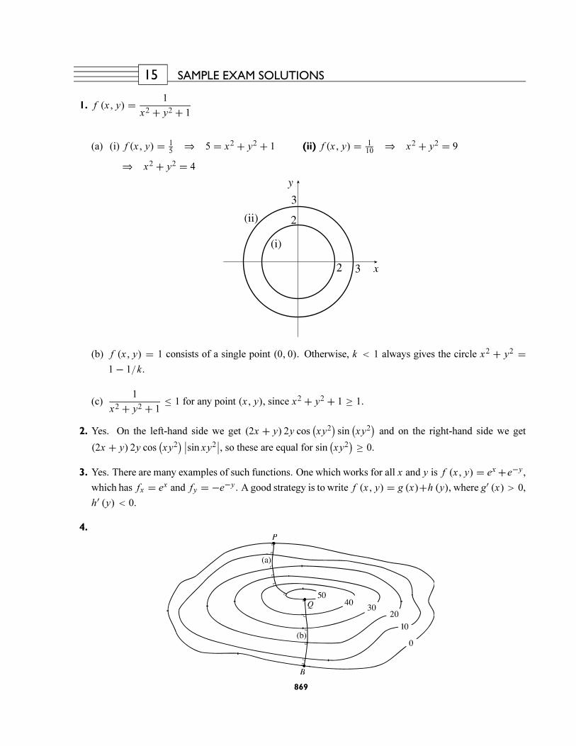
1. f (x, y) = 1
x2 + y2 + 1
(a) (i) f (x, y) = 15
⇒ 5 = x2 + y2 + 1
⇒ x2 + y2 = 4
(ii) f (x, y) = 110
⇒ x2 + y2 = 9
(b) f (x, y) = 1 consists of a single point (0, 0). Otherwise, k < 1 always gives the circle x2 + y2 =1− 1/k.
(c)1
x2 + y2 + 1≤ 1 for any point (x, y), since x2 + y2 + 1 ≥ 1.
2. Yes. On the left-hand side we get (2x + y) 2y cos(xy2)sin(xy2)and on the right-hand side we get
(2x + y) 2y cos(xy2) ∣∣sin xy2∣∣, so these are equal for sin (xy2) ≥ 0.
3. Yes. There are many examples of such functions. One which works for all x and y is f (x, y) = ex +e−y ,
which has fx = ex and fy = −e−y . A good strategy is to write f (x, y) = g (x)+h (y), where g′ (x) > 0,
h′ (y) < 0.
4.
869
CHAPTER 15 PARTIAL DERIVATIVES
5. f (x, y) = x2 + xy + y2 on the disk{(x, y) | x2 + y2 ≤ 9
}.
∇ f (x, y) = 〈2x + y, 2y + x〉 = 〈0, 0〉 ⇔ y = −2x and x = −2y ⇔ (x, y) = (0, 0). So the
minimum value on the interior of the disk is f (0, 0) = 0.
Using Lagrange multipliers for the boundary, we solve ∇ f = λ∇g where g (x, y) = x2 + y2 = 9. So
2x + y = λ2x ⇒ λ = 1 + y/ (2x) and 2y + x = λ2y ⇒ λ = 1 + x/2y ⇒ x2 = y2.
But x2 + y2 = 9, so 2x2 = 9 ⇒ x = ± 3√2and y = ± 3√
2. Thus the maximum value on
the boundary is f(
3√2, 3√
2
)= f
(− 3√
2,− 3√
2
)= 27
2and the minimum value on the boundary is
f(
3√2,− 3√
2
)= f
(− 3√
2, 3√
2
)= 9
2.
The absolute minimum value is f (0, 0) = 0 and the absolute maximum value is f(
3√2, 3√
2
)=
f(− 3√
2,− 3√
2
)= 27
2.
6. (a) Let g (x, y, z) = x2
4+ y2
4+ 2z2, so∇g =
⟨x2,y
2, 4z⟩and ∇g
(√2,√2, 0)=⟨
1√2, 1√
2, 0⟩which is
normal to the surface. So the tangent plane satisfiesx√2+ y√
2= k and goes through
(√2,√2, 0).
Thus k = 1 and the tangent plane isx√2+ y√
2= 1.
(b) Since this is a maximum value of z, the tangent plane is horizontal, that is, z = 1√2. Analytically,
∇g(0, 0, 1√
2
)=⟨0, 0, 2
√2⟩, so the tangent plane is 2
√2z = 2 or z = 1√
2.
7. Ellipsoid for k = −1, single point (0, 0, 0) for k = 1, no surface for k = 2.
8. (a) F (x, y, z) = z
1+ x2 + y2
(b) z = 0 is the only place where F (x, y, z) = 0. So there is no energy on the xy-plane.
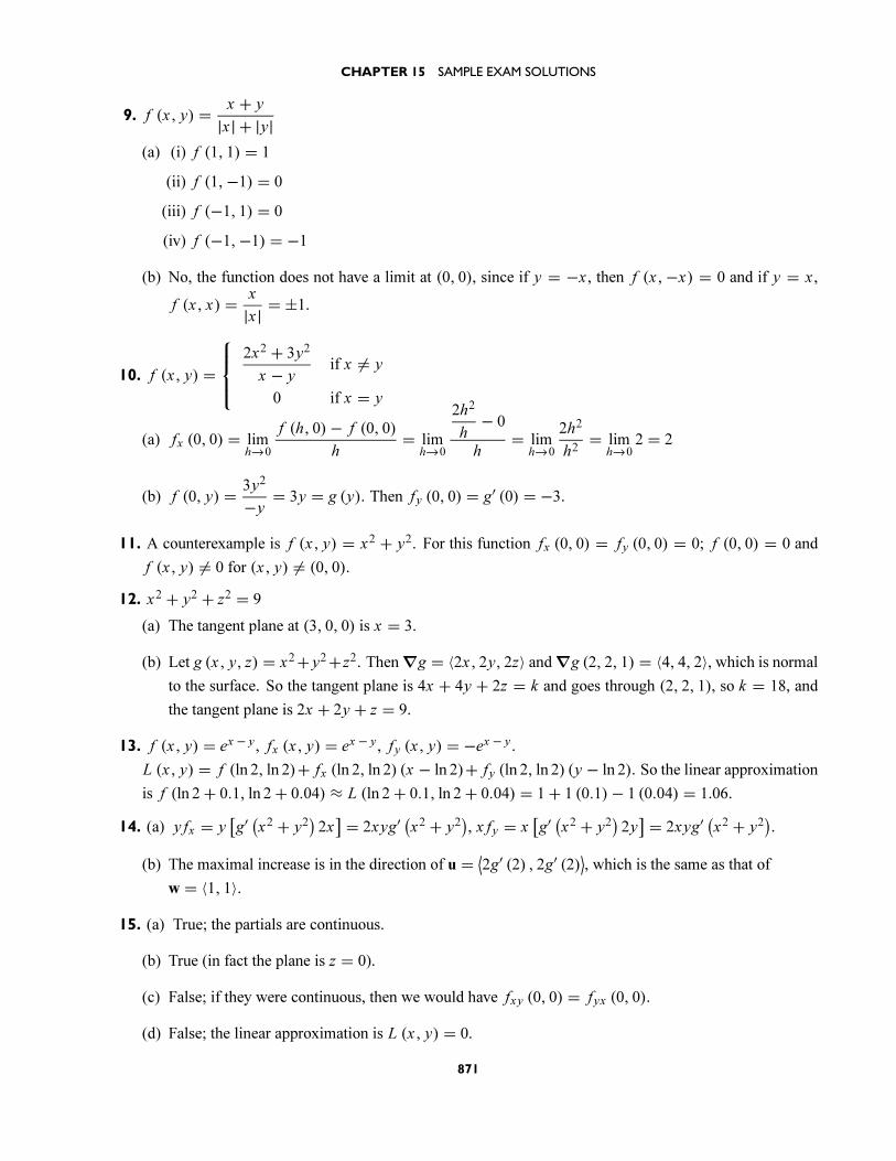
(c) F (x, y, z) = 1 gives 1 = z
1+ x2 + y2or z = 1+ x2 + y2, a circular paraboloid.
870
CHAPTER 15 SAMPLE EXAM SOLUTIONS
9. f (x, y) = x + y
|x | + |y|(a) (i) f (1, 1) = 1
(ii) f (1,−1) = 0
(iii) f (−1, 1) = 0
(iv) f (−1,−1) = −1
(b) No, the function does not have a limit at (0, 0), since if y = −x , then f (x,−x) = 0 and if y = x ,
f (x, x) = x
|x| = ±1.
10. f (x, y) =
⎧⎪⎨⎪⎩
2x2 + 3y2
x − yif x = y
0 if x = y
(a) fx (0, 0) = limh→0
f (h, 0)− f (0, 0)
h= lim
h→0
2h2
h− 0
h= lim
h→0
2h2
h2= lim
h→02 = 2
(b) f (0, y) = 3y2
−y= 3y = g (y). Then fy (0, 0) = g′ (0) = −3.
11. A counterexample is f (x, y) = x2 + y2. For this function fx (0, 0) = fy (0, 0) = 0; f (0, 0) = 0 and
f (x, y) = 0 for (x, y) = (0, 0).
12. x2 + y2 + z2 = 9
(a) The tangent plane at (3, 0, 0) is x = 3.
(b) Let g (x, y, z) = x2+ y2+z2. Then∇g = 〈2x, 2y, 2z〉 and∇g (2, 2, 1) = 〈4, 4, 2〉, which is normal
to the surface. So the tangent plane is 4x + 4y + 2z = k and goes through (2, 2, 1), so k = 18, and
the tangent plane is 2x + 2y + z = 9.
13. f (x, y) = ex − y , fx (x, y) = ex − y , fy (x, y) = −ex − y .
L (x, y) = f (ln 2, ln 2)+ fx (ln 2, ln 2) (x − ln 2)+ fy (ln 2, ln 2) (y − ln 2). So the linear approximation
is f (ln 2+ 0.1, ln 2+ 0.04) ≈ L (ln 2+ 0.1, ln 2+ 0.04) = 1+ 1 (0.1)− 1 (0.04) = 1.06.
14. (a) y fx = y[g′(x2 + y2
)2x] = 2xyg′
(x2 + y2
), x fy = x
[g′(x2 + y2
)2y] = 2xyg′
(x2 + y2
).
(b) The maximal increase is in the direction of u = ⟨2g′ (2) , 2g′ (2)⟩, which is the same as that of
w = 〈1, 1〉.
15. (a) True; the partials are continuous.
(b) True (in fact the plane is z = 0).
(c) False; if they were continuous, then we would have fxy (0, 0) = fyx (0, 0).
(d) False; the linear approximation is L (x, y) = 0.
871
CHAPTER 15 PARTIAL DERIVATIVES
16. u = 〈1, 0〉, v =⟨
1√2, 1√
2
⟩, Du ( f (a, b)) = 3 and Dv ( f (a, b)) =
√2
(a) ∇ f (a, b) = 〈 f1, f2〉 and 〈 f1, f2〉 · u = 3 ⇒ f1 = 3. 〈 f1, f2〉 · v = √2 ⇒ f1√
2+ f2√
2= √
2
⇒ 3√2+ f2√
2= √
2 ⇒ 3+ f2 = 2 ⇒ f2 = −1. So∇ f (a, b) = 〈3,−1〉.
(b) Dw ( f (a, b)) is maximized when w is in the direction of 〈3,−1〉. So w =⟨
3√10,− 1√
10
⟩and since
w = 4√10u− 1√
5v, Dw ( f (a, b)) = 4√
10Du ( f (a, b))− 1√
5Dv ( f (a, b)) = 4√
10· 3− 1√
5·√2 = √
10
(c) Dw ( f (a, b)) = 0 if w · 〈3,−1〉 = 0, so 3w1 − w2 = 0 and w21 + w2
2 = 1 gives w21 + 9w2
1 = 1,
w1 = 1√10
and w2 = 3√10, so w =
⟨1√10, 3√
10
⟩.
17. Since f is a function which is constant on circles x2 + y2 = R and since f is decreasing as the radius of
the circle increases, then the maximum is f (0, 0) = 1 and the minimum is f (4, 3) = e−25.
18. Let d2 = x2 + y2 + z2 and minimize d2 subject to the constraint1
x+ 1
y+ 1
z= 1, x , y, z > 0. The
method of Lagrange multipliers gives the point (3, 3, 3).
872