2005 kirby et al funwave modelformulations (1)
TRANSCRIPT
FUNWAVE 2.0Fully Nonlinear Boussinesq Wave Model
On Curvilinear CoordinatesPart I: Model Formulations
James T. Kirby, Wen Long, Fengyan Shi
Research Report No. CACR-03-xxCenter for Applied Coastal Research
Dept. of Civil & Environmental EngineeringUniversity of Delaware
Newark, Delaware, 19716
May 31, 2005

Contents
1 Introduction 5
2 Original Equations 7
2.1 Equation of Wei et al (1995), O(μ2) . . . . . . . . . . . . . . . . . . . . . 7
2.2 Equations of Andrew Kennedy (2001), O(μ2) . . . . . . . . . . . . . . . . 8
2.3 Equations of Chen et al (2000) , O(μ2) . . . . . . . . . . . . . . . . . . . . 9
3 New Equation Systems 11
3.1 Mauricio F, Gobbi (2000) O(μ4) . . . . . . . . . . . . . . . . . . . . . . . 11
3.2 Kinematics of Potential Theory . . . . . . . . . . . . . . . . . . . . . . . . 21
3.2.1 Horizontal velocity u(x, y, z, t) . . . . . . . . . . . . . . . . . . . . 21
3.2.2 Vertical velocity w(x, y, z, t) . . . . . . . . . . . . . . . . . . . . . . 22
3.2.3 Pressure p(x, y, z, t) . . . . . . . . . . . . . . . . . . . . . . . . . . 22
3.2.4 Flux per unit width . . . . . . . . . . . . . . . . . . . . . . . . . . 24
3.2.5 Ambient current field . . . . . . . . . . . . . . . . . . . . . . . . . . 24
3.2.6 Potential vorticity . . . . . . . . . . . . . . . . . . . . . . . . . . . . 24
3.2.7 Setup-setdown . . . . . . . . . . . . . . . . . . . . . . . . . . . . . 24
3.2.8 Phase velocity, wave direction . . . . . . . . . . . . . . . . . . . . . 24
3.3 Definition of za, zb . . . . . . . . . . . . . . . . . . . . . . . . . . . . . . . 24
4 Derivations from Euler Equation with Vertical Vorticity Retained O(μ2) 25
4.1 Nondimensionalization . . . . . . . . . . . . . . . . . . . . . . . . . . . . 25
4.2 Consistency of Kinematics between Euler Theory and Potential Theory . . 27
4.3 Boussinesq Equation with Vertical Vorticity Retained . . . . . . . . . . . . 31
4.3.1 Continuity equation (COM) . . . . . . . . . . . . . . . . . . . . . . 31
4.3.2 Momentum equation evaluated at z = δη . . . . . . . . . . . . . . . 31
4.3.3 Momentum equation evaluated at arbitrary level z = zc . . . . . . 35
5 Formulations in Curvilinear Coordinates 37
5.1 Final Form of Equations . . . . . . . . . . . . . . . . . . . . . . . . . . . . 37
5.2 Additional Effects for Actual Implementation . . . . . . . . . . . . . . . . 40
5.3 Some Notes on Curvilinear Coordinate . . . . . . . . . . . . . . . . . . . . 43
5.4 Curvilinear Representations of COM and EOM . . . . . . . . . . . . . . . 49
5.5 Curvilinear Representation of Shoreline Boundary Condition . . . . . . . . 60
3
4 CONTENTS
6 Numerics and Programming Details 656.1 Grids and Basic Spatial Difference Schemes . . . . . . . . . . . . . . . . . . 656.2 Flow Chart . . . . . . . . . . . . . . . . . . . . . . . . . . . . . . . . . . . 676.3 Predictor and Corrector . . . . . . . . . . . . . . . . . . . . . . . . . . . . 71
6.3.1 Adams explicit and implicit schemes . . . . . . . . . . . . . . . . . 716.3.2 Implementation of Adams schemes . . . . . . . . . . . . . . . . . . 716.3.3 Hot-Start problem . . . . . . . . . . . . . . . . . . . . . . . . . . . 75
6.4 Obtain u from U . . . . . . . . . . . . . . . . . . . . . . . . . . . . . . . . 766.5 Iteration Error Control and Under-relaxation . . . . . . . . . . . . . . . . . 776.6 Calculation of Kinematics . . . . . . . . . . . . . . . . . . . . . . . . . . . 77
A Wave Maker Theory 79
B Mesh Generator by Fengyan Shi 83
Chapter 1
Introduction
The numerical model FUNWAVE1.0 produced by Center for Applied Coastal Research,1998, is capable of simulating surface waves in coastal region including outer surf zone andinner surf zone. The model is based on theoretical research of Wei et al (1995) in whicha fully nonlinear Boussinesq Equation is set up by extending Nwogu(1993)’s Boussinesqequation with higher order nonlinear dispersive terms retained. The Wei et al(1995) equa-tion can be applied to both intermediate water depth and strong nonlinearity interaction.
After FUNWAVE1.0 was released, further work has been continuously done by Gobbiet al (2000), Kennedy et al(2001), Chen et al (2000), Shi et al(2000), Chawla & Kirby(2000). In Gobbi et al (2000), the equation is extended to fourth order accuracy of dis-persion and multi-reference-level is introduced compared to Nwogu (1993) and Wei etal (1995). In Kennedy(2001), the reference level of Wei et al (1995) is extended to bemoving with the surface elevation. In Chen et al (2000), a second order vertical vorticityterm is further incorporated in the equation which is capable of simulating eddies in thehorizontal plane generated after wave breaking in the surf zone. In Shi et al(2001), theWei et al (1995) equation is solved on curvilinear coordinate system and implemented onstaggered grids to give better accuracy and convergence rate, hence can simulate waveswith complex geometries. In Chawla & Kirby (2000) a one-way wave maker theory forthe model is established by adding a pressure term to the momentum equation comparedto Wei et al (2000).
All these improvements are now put into version 2.0 of FUNWAVE, that is, FUN-WAVE 2.0. In this documentation, a new equation is derived and it’s able to recover allexisting Boussinesq equations above mentioned(Standard Boussinesq, Nwogu 1993, Wei1995, Kennedy 2001, Chen 2000, Gobbi 2000) to the second order of dispersion. And thenew equation is solved on a generalized curvilinear coordinate as Shi(2001). Also internalboundaries of islands, breakwaters ... are included in the new version. In sum the followingare the new features in FUNWAVE 2.0 :
Staggered Grid System
Generalized Curvilinear Coordinate System
Multi-moving-reference-levels
Vertical Vorticity Term Retained
5
6 CHAPTER 1. INTRODUCTION
One-way wave maker
Internal Boundaries
In addition, the new model can output more kinematic and dynamic quantities suchas temporal wave gage, spatial wave gage, pressure, mean current, set-up/set-down, waveheights, potential vorticity.
The breaking simulation, subgrid-mixing, bottom friction, sponge layer, slots(Tao,1983, 1984) method are kept the same as version 1.0.
Detailed derivation of equations, coding, user manual and examples are given in thisdocumentation.

Chapter 2
Original Equations
2.1 Equation of Wei et al (1995), O(μ2)
Continuity of Mass (COM):
ηt + ∇ · M = 0 (2.1)
where
M = (h + δη){uα + μ2[1
2z2
α − 1
6(h2 − hδη + δ2η2)]∇(∇ · uα)
+ μ2[zα +1
2(h − δη)]∇[∇ · (huα)]} + O(μ4)
(2.2)
Equation of Motion (EOM):
uαt + δ(uα · ∇)uα + ∇η + μ2V1 + δμ2V2 = O(μ4) (2.3)
where
V1 =1
2z2
α∇(∇ · uαt) + zα∇[∇ · (huαt)] −∇[1
2(δη)2∇ · uαt + δη∇ · (huαt] (2.4)
V2 = ∇{(zα − δη)(uα · ∇)[∇ · (huα)] +1
2(z2
α − δ2η2)(uα · ∇)(∇ · uα)}
+1
2∇{[∇ · (huα) + δη∇ · uα]2}
(2.5)
δ = a0
h0, μ = k0h0 are scales of nonlinearity and dispersion respectively, where a0 and
h0 are typical wave amplitude and still water depth respectively.
zα = [(1 + 2α)1/2 − 1]h ≈ −0.531h (2.6)
α =1
2(zα
h)2 +
zα
h≈ −0.390 (2.7)
uα is velocity at z = zα: uα = (∇φ)z=zα.
7
8 CHAPTER 2. ORIGINAL EQUATIONS
2.2 Equations of Andrew Kennedy (2001), O(μ2)
Continuity of Mass(COM):
ηt + ∇ · M = 0 (2.8)
where
M = (h + δη){uα + μ2[1
2z2
α − 1
6(h2 − hδη + δ2η2)]∇(∇ · uα)
+ μ2[zα +1
2(h − δη)]∇[∇ · (huα)]} + O(μ4)
(2.9)
(8)(9) are identical to (1)(2). Equation of Motion (EOM):
uαt + δ(uα · ∇)uα + ∇η + μ2V1 + δμ2V2 = O(μ4) (2.10)
where
V1 = [1
2z2
α∇(∇ · uα) + zα∇[∇ · (huα)]]t −∇[1
2(δη)2∇ · uαt + δη∇ · (huαt)] (2.11)
V2 = ∇{(zα − δη)(uα · ∇)[∇ · (huα)] +1
2(z2
α − δ2η2)(uα · ∇)(∇ · uα)}
+1
2∇{[∇ · (huα) + δη∇ · uα]2}
(2.12)
(11) is different from(4) by time derivatives are outside of the square bracket.
zα = ρ0h + β0δη (2.13)
so
zαt = β0δηt (2.14)
Special case:(ρ0 = β0 − 1)
zα = (β0 − 1)h + βδη (2.15)
Set β0 =√
1/5to obtain Pade [2,2] dispersion relation.
Equation (15) is referred as datum invariant version of Boussinesq Equation (Kennedy,2001), for
h + zα
h + δη= β0 = const
When{ρ0 = (1 + 2α)2 − 1 = −0.531;β0 = 0,
(2.16)
we recover WKGS model. When⎧⎨⎩ ρ0 = β0 − 1 =
√1/5 − 1 ≈ −0.5528;
β0 =√
1/5,(2.17)
we recover Kennedy(2001) datum invariant model.

2.3. EQUATIONS OF CHEN ET AL (2000) , O(μ2) 9
2.3 Equations of Chen et al (2000) , O(μ2)
Continuity of Mass(COM):
ηt + ∇ · M = 0 (2.18)
where
M = (h + δη){uα + μ2[1
2z2
α − 1
6(h2 − hδη + δ2η2)]∇(∇ · uα)
+ μ2[zα +1
2(h − δη)]∇[∇ · (huα)]} + O(μ4)
(2.19)
Equation of Motion (EOM):
uαt + δ(uα · ∇)uα + ∇η + μ2V1 + δμ2V2 + δμ2V3 = O(μ4) (2.20)
where
V1 =1
2z2
α∇(∇ · uαt) + zα∇[∇ · (huαt)]] −∇[1
2(δη)2∇ · uαt + δη∇ · (huαt)] (2.21)
V2 = ∇{(zα − δη)(uα · ∇)[∇ · (huα)] +1
2(z2
α − δ2η2)(uα · ∇)(∇ · uα)}
+1
2∇{[∇ · (huα) + δη∇ · uα]2}
(2.22)
and
V3 = (V x3 , V y
3 ) = Ω1 × uα (2.23)
V x3 = −vαω1; v
y3 = uαω1 (2.24)
Ω1 = (0, 0, ω1) (2.25)
ω1 = zαx{[∇ · (huα)]y + zα(∇ · uα)y}− zαy{[∇ · (huα)]x − zα(∇ · uα)x}
(2.26)
Chen et al (2000) equation has an extra term V3 compared to Wei et al (1995), whichis the second order correction of vertical vorticity evaluated at z = zα :
ω|z=zα = ω0 + μ2ω1 = (∇× u)|z=zα (2.27)
where
ω0 = ∇× uα (2.28)

10 CHAPTER 2. ORIGINAL EQUATIONS
ω1 = {∇ × (u− uα)}|z=zα (2.29)
u = uα
+ μ2{(zα − z)∇[∇ · (huα)]
+ (z2
α
2− z2
2)∇(∇ · uα)}
(2.30)

Chapter 3
New Equation Systems
3.1 Mauricio F, Gobbi (2000) O(μ4)
This section gives derivations from potential flow theory.
Governing Equation:COM:
ηt + ∇ · M = 0,M =∫ δη
−h∇φdz (3.1)
Laplace:
φzz + μ2∇2φ = 0; −h ≤ z ≤ δη (3.2)
Bottom Boundary Condition(BBC):
φz + μ2∇h · ∇φ = 0; z = −h (3.3)
Dynamic Free Surface Boundary Condition(DFSBC):
η + φt +1
2δ[(∇φ)2 +
1
μ2(φz)
2] = 0; z = δη (3.4)
Kinematic Free Surface Boundary Condition(KFSBC):
ηt + δ∇φ · ∇η − 1
μ2φz = 0; z = δη (3.5)
Introducing Taylor expansion:
φ(x, y, z, t) =N∑
n=0
ξnφn(x, y, t) (3.6)
From BBC, we get:
φ1 = −μ2G∇h · ∇φ0 (3.7)
where
G =1
1 + μ2|∇h|2 (3.8)
11

12 CHAPTER 3. NEW EQUATION SYSTEMS
From Laplace equation,
(n + 2)(n + 1)φn+2 + μ2[(n + 2)(n + 1)|∇h|2φn+2 + (n + 1)∇2hφn+1
+ 2(n + 1)∇h · ∇φn+1 + ∇2φn] = 0 (n = 0, 1, 2, ...)
(3.9)
From the last 3 equations above, we get:
φ2 = −μ2
2G∇2φ0 + μ4[
G2
2∇2h∇h · ∇φ0 + G∇h · ∇(G∇h · ∇φ0)] + O(μ6) (3.10)
φ3 = μ4[G2∇2h∇2φ0
6+
1
3G∇h · ∇(G∇2φ0) +
1
6G∇2(G∇h · ∇φ0)] + O(μ2) (3.11)
φ4 =μ4
24G∇2(G∇2φ0) + O(μ6) (3.12)
so,
φ = φ0 + φ1ξ + φ2ξ2 + φ3ξ
3 + φ4ξ4 + ...
= φ0 − μ2G∇h · ∇φ0ξ − μ2
2G∇2φ0ξ
2
+ μ4[G2
2∇2h∇h · ∇φ0 + G∇h · ∇(G∇h · ∇φ0)]ξ
2
+ μ4[G2∇2h∇2φ0
6+
1
3G∇h · ∇(G∇2φ0) +
1
6G∇2(G∇h · ∇φ0)]ξ
3
+ [μ4
24G∇2(G∇2φ0) + O(μ6)]ξ4
+ O(μ6)
(3.13)
Introduce
φ = βφa + (1 − β)φb (3.14)
where φa, φb are φ at za, zb respectively.In GKW98, the definitions of za, zb are:
za = {[19− { 8β
567(1− β)}1/2 + { 8
567β(1− β)}1/2]1/2 − 1}h (3.15)
zb = {[19− { 8β
567(1 − β)}1/2]1/2 − 1}h (3.16)
β ≈ 0.2 (3.17)
Plugging φa and φb into φ, one obtains:
3.1. MAURICIO F, GOBBI (2000) O(μ4) 13
φ = φ0 − μ2(AhG∇h · ∇φ0 +1
2Bh2G∇2φ0)
+ μ4{Bh2[1
2G2∇2h∇h · ∇φ0 + G∇h · ∇(G∇h · ∇φ0)]
+ Ch3[1
6G2∇2h∇2φ0 +
1
3G∇h · ∇(G∇2φ0) +
1
6G∇2(G∇h · ∇φ0)]
+ Dh4 1
24G∇2(G∇2φ0)}
+ O(μ6)
(3.18)
where
⎧⎪⎪⎪⎨⎪⎪⎪⎩
A = 1h[β(h + za) + (1 − β)(h + zb)]
B = 1h2 [β(h + za)
2 + (1 − β)(h + zb)2]
C = 1h3 [β(h + za)
3 + (1 − β)(h + zb)3]
D = 1h4 [β(h + za)
4 + (1 − β)(h + zb)4]
(3.19)
Inverse the equation above, we get φ0 in terms of φ :
φ0 = φ + μ2[AhG∇h · ∇φ +1
2Bh2G∇2φ]
+ μ4[AhG∇h · ∇(AhG∇h · ∇φ +1
2Bh2G∇2φ)
+1
2Bh2G∇2(AhG∇h · ∇φ +
1
2Bh2G∇2φ)]
− μ4{Bh2[1
2G2∇2h∇h · ∇φ + G∇h · ∇(G∇h · ∇φ)]
+ Ch3[1
6G2∇2h∇2φ +
1
3G∇h · ∇(G∇2φ) +
1
6G∇2(G∇h · ∇φ)]
+ Dh4 1
24G∇2(G∇2φ)}
+ O(μ6)
(3.20)
Plug it into (3.13), we have:
φ = φ + μ2[(Ah − ξ)F1 + (Bh2 − ξ2)F2]
+ μ4[(Ah − ξ)F3 + (Bh2 − ξ2)F4) + (Ch3 − ξ3)F5 + (Dh4 − ξ4)F6]
(3.21)

14 CHAPTER 3. NEW EQUATION SYSTEMS
Where
⎧⎪⎪⎪⎪⎪⎪⎪⎪⎪⎪⎪⎪⎪⎪⎪⎪⎪⎪⎪⎪⎪⎪⎨⎪⎪⎪⎪⎪⎪⎪⎪⎪⎪⎪⎪⎪⎪⎪⎪⎪⎪⎪⎪⎪⎪⎩
F1 = G∇h · ∇φ
F2 = 12G∇2φ
F3 = ∇h · ∇(Ah∇h · ∇φ) + 12∇h · ∇(Bh2∇2φ)
F4 = 12∇2(Ah∇h · ∇φ)
+14∇2(Bh2∇2φ)
−12∇2h∇h · ∇φ
−∇h · ∇(∇h · ∇φ)
F5 = −16∇2h∇2φ
−13∇h · ∇(∇2φ)
−16∇2(∇h · ∇φ)
F6 = − 124∇2(∇2φ)
(3.22)
Then,
u = ∇φ = ∇φ
+ μ2[(∇(AhF1) − ξ∇F1 − F1∇h)
+ (∇(Bh2F2) − ξ2∇F2 − 2ξF2∇h)]
+ μ4[(∇(AhF3) − ξ∇F3 − F3∇h)
+ (∇(Bh2F4) − ξ2∇F4 − 2ξF4∇h)
+ (∇(Ch3F5) − ξ3∇F5 − 3ξ2F5∇h)
+ (∇(Dh4F6) − ξ4∇F6 − 4ξ3F6∇h)]
(3.23)
Plug this equation into
M =∫ δη
−h∇φdz =
∫ H
0∇φdξ
then
M = H∇φ
+ μ2H{∇(AhF1) − H
2∇F1 − F1∇h
+ ∇(Bh2F2) − H2
3∇F2 − HF2∇h}
+ μ4 H{∇(AhF3) − H
2∇F3 − F3∇h
+ ∇(Bh2F4) − H2
3∇F4 − HF4∇h
+ ∇(Ch3F5) − H3
4∇F5 − H2F5∇h
+ ∇(Dh4F6) − H4
5∇F6 − H3F6∇h}
3.1. MAURICIO F, GOBBI (2000) O(μ4) 15
(3.24)
Plug (51) into DFSBC and then evaluate it at ξ = H , we get
η + φt +1
2δ|∇φ|2
+ μ2[(AthF1 + (Ah − H)F1t) + (Bth2F2 + (Bh2 − H2)F2t)]
+ δμ2[∇φ · {∇((Ah − H)F1) + F1∇δη
+ ∇((Bh2 − H2)F2) + 2F2H∇δη}+
1
2(F1 + 2HF2)
2]
+ μ4[(AthF3 + (Ah − H)F3t) + (Bth2F4 + (Bh2 − H2)F4t)
+ (Cth3F5 + (Ch3 − H3)F5t + (Dth
4F6 + (Dh4 − H4)F6t)]
+ δμ4[1
2|∇((Ah − H)F1) + F1∇δη + ∇((Bh2 − H2)F2) + 2F2H∇δη|2
+ ∇φ · [∇((Ah − H)F3) + F3∇δη + ∇((Bh2 − H2)F4) − 2F4H∇δη
+ ∇((Ch3 − H3)F5) + 3F5H2∇δη + ∇((Dh4 − H4)F6) − 4F6H
3∇δη]
+ (F1 + 2HF2)(F3 + 2HF4 + 3H2F5 + 4H3F6)}= O(μ6)
(3.25)
Introduce:
u(x,y, t) = βua + (1 − β)ub
= β[∇φ]|z=za + (1 − β)[∇φ]|z=zb
(3.26)
where
[∇φ]|z=za = ∇φ
+ μ2[(∇(AhF1) − (h + za)∇F1 − F1∇h)
+ (∇(Bh2F2) − (h + za)2∇F2 − 2(h + za)F2∇h)]
+ μ4[(∇(AhF3) − (h + za)∇F3 − F3∇h)
+ (∇(Bh2F4) − (h + za)2∇F4 − 2(h + za)F4∇h)
+ (∇(Ch3F5) − (h + za)3∇F5 − 3(h + za)
2F5∇h)
+ (∇(Dh4F6) − (h + za)4∇F6 − 4(h + za)
3F6∇h)]
(3.27)
[∇φ]|z=zbis similar. Thus,
u = βua + (1 − β)ub
= ∇φ + μ2[F1∇(Ah − h) + F2(∇(Bh2) − 2Ah∇h)]
+ μ4[F3∇(Ah − h) + F4(∇(Bh2) − 2Ah∇h)
+ F5(∇(Ch3) − 3Bh2∇h) + F6(∇(Dh4) − 4h3(∇h)]
+ O(μ6)
16 CHAPTER 3. NEW EQUATION SYSTEMS
(3.28)
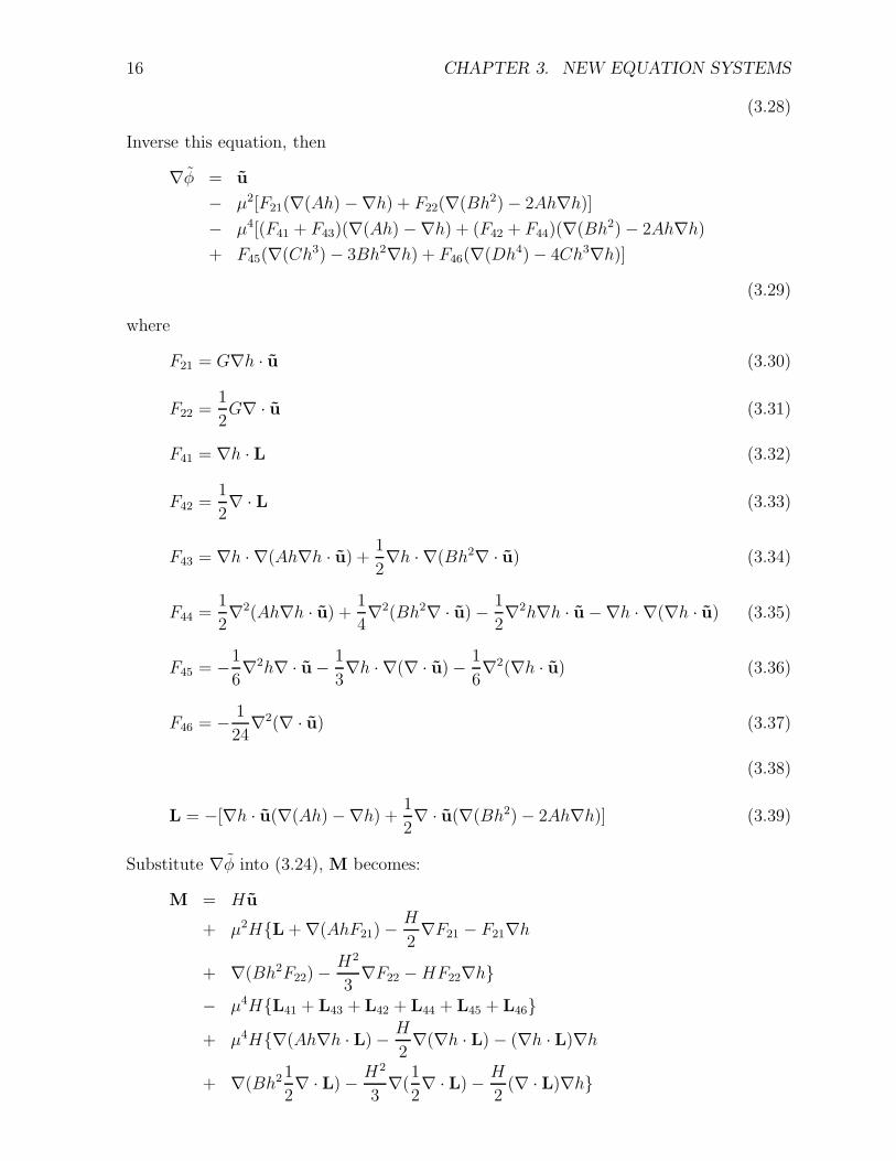
Inverse this equation, then
∇φ = u
− μ2[F21(∇(Ah) −∇h) + F22(∇(Bh2) − 2Ah∇h)]
− μ4[(F41 + F43)(∇(Ah) −∇h) + (F42 + F44)(∇(Bh2) − 2Ah∇h)
+ F45(∇(Ch3) − 3Bh2∇h) + F46(∇(Dh4) − 4Ch3∇h)]
(3.29)
where
F21 = G∇h · u (3.30)
F22 =1
2G∇ · u (3.31)
F41 = ∇h · L (3.32)
F42 =1
2∇ · L (3.33)
F43 = ∇h · ∇(Ah∇h · u) +1
2∇h · ∇(Bh2∇ · u) (3.34)
F44 =1
2∇2(Ah∇h · u) +
1
4∇2(Bh2∇ · u) − 1
2∇2h∇h · u −∇h · ∇(∇h · u) (3.35)
F45 = −1
6∇2h∇ · u− 1
3∇h · ∇(∇ · u) − 1
6∇2(∇h · u) (3.36)
F46 = − 1
24∇2(∇ · u) (3.37)
(3.38)
L = −[∇h · u(∇(Ah) −∇h) +1
2∇ · u(∇(Bh2) − 2Ah∇h)] (3.39)
Substitute ∇φ into (3.24), M becomes:
M = Hu
+ μ2H{L + ∇(AhF21) − H
2∇F21 − F21∇h
+ ∇(Bh2F22) − H2
3∇F22 − HF22∇h}
− μ4H{L41 + L43 + L42 + L44 + L45 + L46}+ μ4H{∇(Ah∇h · L) − H
2∇(∇h · L) − (∇h · L)∇h
+ ∇(Bh21
2∇ · L) − H2
3∇(
1
2∇ · L) − H
2(∇ · L)∇h}

3.1. MAURICIO F, GOBBI (2000) O(μ4) 17
+ μ4H{∇(AhF43) − H
2∇F43 − F43∇h
+ ∇(Bh2F44) − H2
3∇F44 − HF44∇h
+ ∇(Ch3F45) − H3
4∇F45 − H2F45∇h
+ ∇(Dh4F46) − H4
5∇F46 − H3F46∇h}
+ O(μ6)
(3.40)
where
L41 = F41A1 ;L42 = F42B1
L43 = F43A1 ;L44 = F44B1
L45 = F45C1 ;L46 = F46D1
A1 = ∇(Ah) −∇h ;B1 = ∇(Bh2) − 2Ah∇h
C1 = ∇(Ch3) − 3Bh2∇h ;D1 = ∇(Dh4) − 4Ch3∇h
L21 = F21A1 ;L22 = F22B1
L = −(L21 + L22)
∇h · L = F41 ;∇h · L = F42
(3.41)
A simplification by some algebra leads to
M = H{u+ μ2[(Ah − H
2)(2∇hF22 + ∇F21) + (Bh2 − H2
3)∇F22]
+ μ4[(Ah − H
2)(2∇hF42 + ∇F41 + 2∇hF44 + ∇F43)
+ (Bh2 − H2
2)(∇F42 + 3∇hF45 + ∇F44)
+ (Ch3 − H3
4)(4∇hF46 + ∇F45) + (Dh4 − H4
5)∇F46]}
+ O(μ6)
(3.42)

18 CHAPTER 3. NEW EQUATION SYSTEMS
Take gradient to Bernoulli Equation (3.25) , we obtain
∇η + (∇φ)t +1
2δ∇|∇φ|2
+ μ2[∇(AthF1) + ∇((Ah − H)F1t)
+ ∇(Bth2F2) + ∇((Bh2 − H2)F2t)]
+ δμ2{∇[∇φ · [∇((Ah − H)F1 + F1δη
+ ∇((Bh2 − H2)F2) + 2F2H∇δη]]
+1
2∇(F1 + 2HF2)
2}+ μ4[∇(AthF3 + (Ah − H)F3t) + ∇(Bth
2F4 + (Bh2 − H2)F4t)
+ ∇(Cth3F5 + (Ch3 − H3)F5t) + ∇(Dth
4F6 + (Dh4 − H4)F6t)]
+1
2δμ4∇|∇((Ah − H)F1) + F1∇δη
+ ∇((Bh2 − H2)F2) + 2F2H∇δη|2+ δμ4∇{∇φ · [∇((Ah − H)F3) + F3∇δη
+ ∇((Bh2 − H2)F4) + 2F4H∇δη
+ ∇((Ch3 − H3)F5) + 3F5H2∇δη
+ ∇((Dh4 − H4)F6) + 4F6H3∇δη]}
+ δμ4∇{(F1 + 2HF2)(F3 + 2HF4 + 3H2F5 + 4H3F6)}= O(μ6)
(3.43)
Substitute (3.29) into this equation, then
ut − μ2[−Lt]
+ μ2[∇(AthF21) + ∇((Ah − H)F21t)
+ ∇(Bth2F22) + ∇((Bh2 − H2)F22t)]
+ μ4[L41t + L43t + L42t + L44t + L45t + L46t]
− μ4[−∇(Ath∇h · L) −∇((Ah − H)∇h · Lt)
− ∇(Bth2 1
2∇ · L) −∇((Bh2 − H2)
1
2∇ · Lt)]
+ μ4[∇(AthF43 + (Ah − H)F43t) + ∇(Bth2F44 + (Bh2 − H2)F44t)
+ ∇(Cth3F45 + (Ch3 − H3)F45t) + ∇(Dth
4F46 + (Dh4 − H4)F46t)]
= − ∇η − 1
2δ∇|u|2 + δμ2[−∇(u · L)]
− δμ2{∇[u · [∇((Ah − H)F21) + ∇((Bh2 − H2)F22)
+ F21∇δη + 2HF22∇δη]] +1
2∇(F21 + 2HF22)
2}
− δμ4{1
2∇|L|2
− ∇(u · [L41 + L43 + L42 + L44 + L45 + L46])}− δμ4{∇{u · [∇((Ah − H)∇h · L) + ∇h · L∇δη

3.1. MAURICIO F, GOBBI (2000) O(μ4) 19
+ ∇ · ((Bh2 − H2)1
2∇ · L) + ∇ · LH∇δη]}
+ ∇{L · [∇((Ah − H)F21 + F21∇δη
+ ∇((Bh2 − H2)F22 + 2HF22∇δη]}+
1
2∇{2F21∇h · L + 4H2F22∇ · L
+ 2HF21∇ · L + 4HF22∇h · L}}− 1
2δμ4∇|∇((Ah − H)F21) + F21∇δη
+ ∇((Bh2 − H2)F22) + 2HF22∇δη|2− δμ4∇{u · [∇((Ah − H)F43) + F43∇δη
+ ∇((Bh2 − H2)F42) + 2F44H∇δη
+ ∇((Ch3 − H3)F45) + 3F45H2∇δη
+ ∇((Dh4 − H4)F46) + 4F46H3∇δη]}
− δμ4∇{(F21 + 2HF22)(F43 + 2HF44 + 3H2F45 + 4H3F46)}+ O(μ6)
(3.44)
Utilizing F42 = 12∇ · L, F41 = ∇h · L, the upper equation can be simplified as:
Ut = −∇η − δ
2∇(|u|2) + Γ1 + Γ2 (3.45)
where
U = u
+ μ2[(A − 1)h(2∇hF22 + ∇F21) + (B − 1)h2∇F22]
+ μ4[(A − 1)h(2∇hF42 + ∇F41 + 2∇hF44 + ∇F43)
+ (B − 1)h2(∇F42 + 3∇hF45 + ∇F44)
+ (C − 1)h3(4∇hF46 + ∇F45)
+ (D − 1)h4∇F46]
(3.46)
Γ1 = μ2∇[δηF21t + (2hδη + δ2η2)F22t]
+ μ4∇[δη(F41t + F43t) + (2hδη + δ2η2)(F42t + F44t)
+ (3h2δη + 3hδ2η2 + δ3η3)F45t
+ (4h3δη + 6h2δ2η2 + 4hδ3η3 + δ4η4)F46t]
(3.47)
Γ2 = −δμ2∇{u · [(Ah − H)(∇F21 + 2∇hF22)
+ (Bh2 − H2)∇F22] +1
2(F21 + 2HF22)
2}
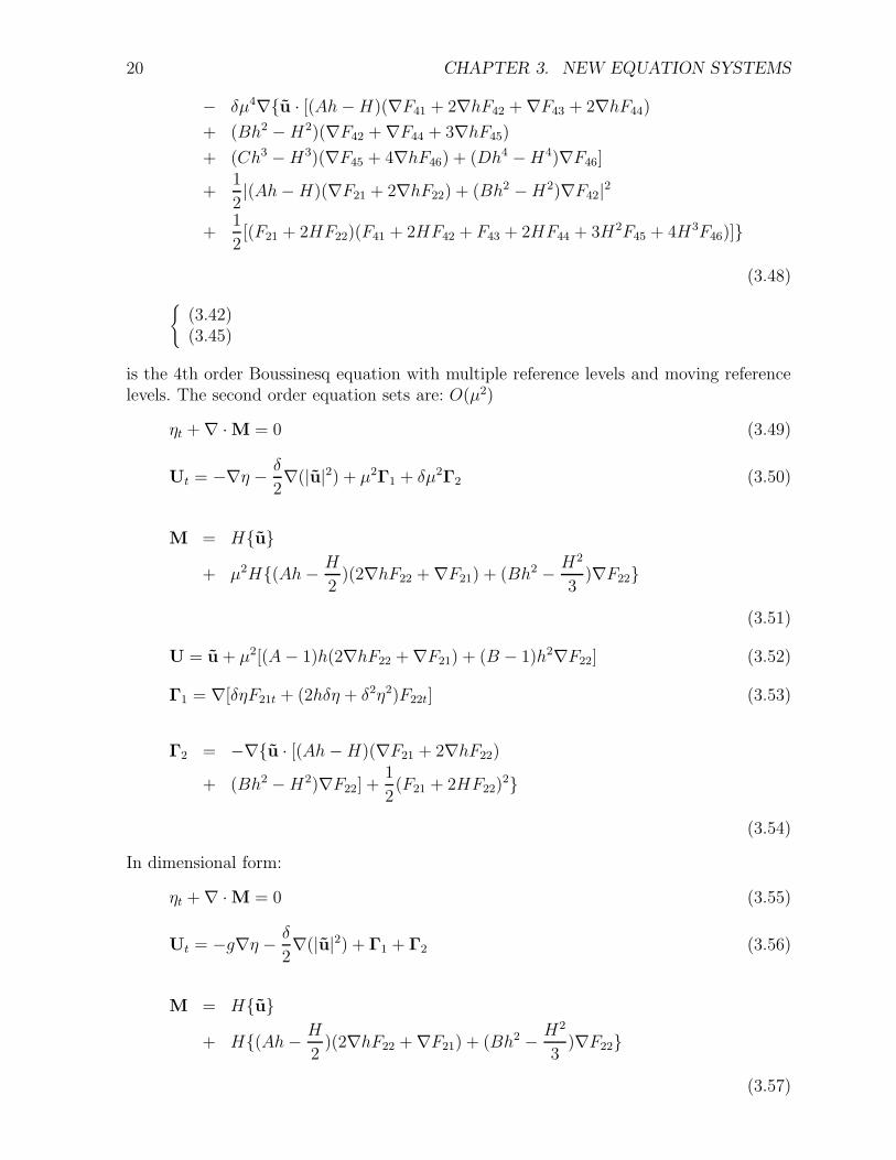
20 CHAPTER 3. NEW EQUATION SYSTEMS
− δμ4∇{u · [(Ah − H)(∇F41 + 2∇hF42 + ∇F43 + 2∇hF44)
+ (Bh2 − H2)(∇F42 + ∇F44 + 3∇hF45)
+ (Ch3 − H3)(∇F45 + 4∇hF46) + (Dh4 − H4)∇F46]
+1
2|(Ah − H)(∇F21 + 2∇hF22) + (Bh2 − H2)∇F42|2
+1
2[(F21 + 2HF22)(F41 + 2HF42 + F43 + 2HF44 + 3H2F45 + 4H3F46)]}
(3.48)
{(3.42)(3.45)
is the 4th order Boussinesq equation with multiple reference levels and moving referencelevels. The second order equation sets are: O(μ2)
ηt + ∇ · M = 0 (3.49)
Ut = −∇η − δ
2∇(|u|2) + μ2Γ1 + δμ2Γ2 (3.50)
M = H{u}+ μ2H{(Ah − H
2)(2∇hF22 + ∇F21) + (Bh2 − H2
3)∇F22}
(3.51)
U = u + μ2[(A − 1)h(2∇hF22 + ∇F21) + (B − 1)h2∇F22] (3.52)
Γ1 = ∇[δηF21t + (2hδη + δ2η2)F22t] (3.53)
Γ2 = −∇{u · [(Ah − H)(∇F21 + 2∇hF22)
+ (Bh2 − H2)∇F22] +1
2(F21 + 2HF22)
2}
(3.54)
In dimensional form:
ηt + ∇ · M = 0 (3.55)
Ut = −g∇η − δ
2∇(|u|2) + Γ1 + Γ2 (3.56)
M = H{u}+ H{(Ah − H
2)(2∇hF22 + ∇F21) + (Bh2 − H2
3)∇F22}
(3.57)
3.2. KINEMATICS OF POTENTIAL THEORY 21
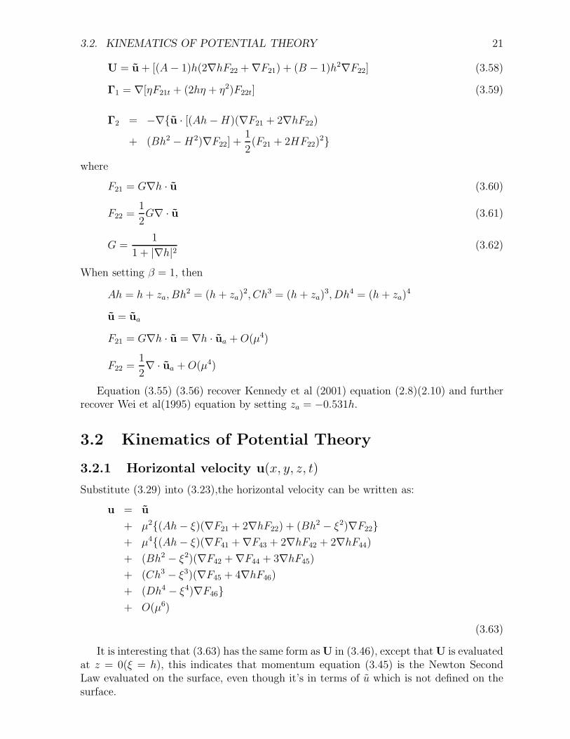
U = u + [(A − 1)h(2∇hF22 + ∇F21) + (B − 1)h2∇F22] (3.58)
Γ1 = ∇[ηF21t + (2hη + η2)F22t] (3.59)
Γ2 = −∇{u · [(Ah − H)(∇F21 + 2∇hF22)
+ (Bh2 − H2)∇F22] +1
2(F21 + 2HF22)
2}
where
F21 = G∇h · u (3.60)
F22 =1
2G∇ · u (3.61)
G =1
1 + |∇h|2 (3.62)
When setting β = 1, then
Ah = h + za, Bh2 = (h + za)2, Ch3 = (h + za)
3, Dh4 = (h + za)4
u = ua
F21 = G∇h · u = ∇h · ua + O(μ4)
F22 =1
2∇ · ua + O(μ4)
Equation (3.55) (3.56) recover Kennedy et al (2001) equation (2.8)(2.10) and furtherrecover Wei et al(1995) equation by setting za = −0.531h.
3.2 Kinematics of Potential Theory
3.2.1 Horizontal velocity u(x, y, z, t)
Substitute (3.29) into (3.23),the horizontal velocity can be written as:
u = u
+ μ2{(Ah − ξ)(∇F21 + 2∇hF22) + (Bh2 − ξ2)∇F22}+ μ4{(Ah − ξ)(∇F41 + ∇F43 + 2∇hF42 + 2∇hF44)
+ (Bh2 − ξ2)(∇F42 + ∇F44 + 3∇hF45)
+ (Ch3 − ξ3)(∇F45 + 4∇hF46)
+ (Dh4 − ξ4)∇F46}+ O(μ6)
(3.63)
It is interesting that (3.63) has the same form as U in (3.46), except that U is evaluatedat z = 0(ξ = h), this indicates that momentum equation (3.45) is the Newton SecondLaw evaluated on the surface, even though it’s in terms of u which is not defined on thesurface.

22 CHAPTER 3. NEW EQUATION SYSTEMS
3.2.2 Vertical velocity w(x, y, z, t)
w(x, y, z, t) = φz
= μ2(−F1 − 2ξF2)
+ μ4(−F3 − 2ξF4 − 3ξ2F5 − 4ξ3F6)
(3.64)
where F1, F2, F3, F4, F5, F6 are all in terms of ∇φ. Plug (3.29) in to the upper equation,we have
w(x, y, z, t) = − μ2(F21 + 2ξF22)
− μ4(F41 + F43 + 2ξF42 + 2ξF44 + 3ξ2F45 + 4ξ3F46
(3.65)
Also interestingly (3.65) is hidden in Γ2 of momentum equation(3.48), but evaluatedat ξ = H there!
3.2.3 Pressure p(x, y, z, t)
From Euler equation:
wt + δuwx + δvwy = −pz − 1
δ(3.66)
i.e.
−pz =1
δ+ wt + δu · ∇w (3.67)
Substitute (3.63)(3.65) into it, we have:
−pz =1
δ− μ2[F21t + 2ξF22t + δu · (∇F21 + 2ξ∇F22 + 2F22∇h)]
− μ4{(F41t + F43t + 2ξF42t + 2ξF44t + 3ξ2F45t + 4ξ3F46t)
+ δu · (∇F41 + ∇F43 + 2ξ∇F42 + 2ξ∇F44 + 3ξ2∇F45
+ 4ξ3∇F46 + 6ξF45∇h + 12ξ2F46∇h)
+ δ(Ah − ξ)(∇F21 + 2∇hF22) · (∇F21 + 2F22∇h)
+ δ2(Ah − ξ)ξ(∇F21 + 2∇hF22) · ∇F22
+ δ(Bh2 − ξ2)∇F22 · (∇F21 + 2∇hF22)
+ δ2ξ(Bh2 − ξ2)∇F22 · ∇F22}+ O(μ6)
(3.68)

3.2. KINEMATICS OF POTENTIAL THEORY 23
Integrate it from surface to z, we obtain:
p − pa = η − z
δ− μ2{(H − ξ)F21t + (H2ξ2)F22t
+ δu · [∇F21(H − ξ) + ∇F22(H2 − ξ2) + 2F22∇h(H − ξ)]}
− μ4{(F41t + F43t)(H − ξ) + (F42t + F44t)(H2 − ξ2)
+ 2(H − ξ)(F42 + F44)∇h
+ F45t(H3 − ξ3) + F46t(H
4 − ξ4)
+ δu · [(H − ξ)(∇F41 + ∇F43)
+ (H2 − ξ2)(∇F42 + ∇F44)
+ (H3 − ξ3)∇F45 + (H4 − ξ4)∇F46
+ 3(H2 − ξ2)F45∇h + 4(H3 − ξ3)F46∇h]
+ δ[Ah(H − ξ) − (H2 − ξ2)
2](∇F21 + 2∇hF22)
· (∇F21 + 2F22∇h)
+ δ[Ah(H2 − ξ2) + Bh2(H − ξ) − (H3 − ξ3)]∇F22
· (∇F21 + 2∇hF22)
+ δ[Bh2(H2 − ξ2) +1
2(H4 − ξ4)]∇F22 · ∇F22}
+ Oμ6
(3.69)
where pa is pressure on the surface.
In summary, for second order approximation,
u = u + μ2{(Ah − ξ)(∇F21 + 2∇hF22) + (Bh2 − ξ2)∇F22} (3.70)
w(x, y, z, t) = −μ2(F21 + 2ξF22) (3.71)
p = pa + η − z
δ− μ2{(δη − z)F21t + (H2 − ξ2)F22t
+ δu · [∇F21(δη − z) + ∇F22(H2 − ξ2) + 2F22∇h(δη − z)]}
(3.72)
In dimensional form:
u = u + {(Ah − ξ)(∇F21 + 2∇hF22) + (Bh2 − ξ2)∇F22} (3.73)
w(x, y, z, t) = −(F21 + 2ξF22) (3.74)
p = pa + ρg(η − z)
− ρ{(η − z)F21t + (H2 − ξ2)F22t
+ u · [∇F21(η − z) + ∇F22(H2 − ξ2) + 2F22∇h(η − z)]}
(3.75)
24 CHAPTER 3. NEW EQUATION SYSTEMS
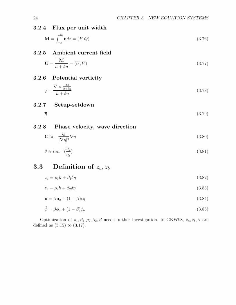
3.2.4 Flux per unit width
M =∫ δη
−hudz = (P, Q) (3.76)
3.2.5 Ambient current field
U =M
h + δη= (U, V ) (3.77)
3.2.6 Potential vorticity
q =∇× M
h+δη
h + δη(3.78)
3.2.7 Setup-setdown
η (3.79)
3.2.8 Phase velocity, wave direction
C ≈ − ηt
|∇η|2∇η (3.80)
θ ≈ tan−1(ηy
ηx) (3.81)
3.3 Definition of za, zb
za = ρ1h + β1δη (3.82)
zb = ρ2h + β2δη (3.83)
u = βua + (1 − β)ub (3.84)
φ = βφa + (1 − β)φb (3.85)
Optimization of ρ1, β1, ρ2, β2, β needs further investigation. In GKW98, za, zb, β aredefined as (3.15) to (3.17).
Chapter 4
Derivations from Euler Equationwith Vertical Vorticity RetainedO(μ2)
4.1 Nondimensionalization
Define the following nodimensional variables:
x′ = k0x, y′ = k0y, z′ = z/h0, t′ = k0C0t
η′ = η/a0, h′ = h/h0
(4.1)
where ()’ means nodimensional quantities ,and () means dimensional quantities. Then,
φ′ =φ
φ0
φ0 =a0l0C0
2πh0
(u′, v′) =h0
a0C0
(u, v)w′ =2πh2
0
a0l0C0
wp′ =p
ρga0
(4.2)
where l0 is typical wave length, l0 = 2π/k0; C0 is typical phase speed, C0 =√
gh0; h0 istypical water depth; a0 is typical wave amplitude; k0 is typical wave number.
Governing Equation for Potential Flow repeated here:Laplace:
φxx + φyy + φzz = 0,−h ≤ z ≤ η (4.3)
BBC:
φz + ∇h · ∇φ = 0, z = −h (4.4)
DFSBC:
φt +1
2(∇φ)2 + gη = 0, z = η (4.5)
KFSBC:
ηt + ∇φ · ∇η = φz, z = η (4.6)
25

26CHAPTER 4. DERIVATIONS FROM EULER EQUATION WITH VERTICAL VORTICITY RETA
Non-dimensional form (primes are dropped):Laplace:
μ2∇2φ + φzz = 0,−h ≤ z ≤ δη (4.7)
BBC:
φz + μ2∇h · ∇φ = 0, z = −h (4.8)
DFSBC:
η + φt +1
2δ[(∇φ)2 +
1
μ2(φz)
2] = 0, z = δη (4.9)
KFSBC:
ηt + δ∇φ · ∇η − 1
μ2φz = 0, z = δη (4.10)
where μ2 = k0h0 is dispersion index and δ = a0/h0 is nonlinearity index.Governing Equation from Eulerian Point of View
COM:
∇ · u = ux + vy + wz = 0 (4.11)
EOM:
x : ut + uux + vuy + wuz = −1
ρpx (4.12)
y : vt + uvx + vvy + wvz = −1
ρpy (4.13)
z : wt + uwx + vwy + wwz = −1
ρpz − g (4.14)
Nondimensional form:COM:
μ2ux + μ2vy + wz = 0 (4.15)
EOM:
Du
Dt+ ∇p = 0 (4.16)
Dw
Dt+ pz + 1/δ = 0 (4.17)
where
D
Dt=
∂
∂t+ δ(u · ∇) +
δ
μ2w
∂
∂z(4.18)
u = (u, v),∇ = (∂
∂x,
∂
∂y) (4.19)
4.2. CONSISTENCY OF KINEMATICS BETWEEN EULER THEORY AND POTENTIAL THEORY
Boundary Condition (BC):KFSBC:
μ2∂η
∂t+ δη2ui
∂η
∂xi− w = 0, z = δη (4.20)
DFSBC:
p = pa = 0, z = δη (4.21)
BBC:
μ2ui∂h
∂xi+ w = 0, z = −h (4.22)
Non-horizontal vorticity:
∂ui
∂z− ∂w
∂xi= 0,−h ≤ z ≤ δη (4.23)
4.2 Consistency of Kinematics between Euler Theory
and Potential Theory
Integrate COM from z = −h to z , we obtain:
∫ z
−hμ2 ∂ui
∂xi
dz +∫ z
−h
∂w
∂zdz = 0 (4.24)
Utilizing Leibniz’s Rule, the upper equation becomes:
μ2 ∂
∂xi
∫ z
−huidz + w|z − [μ2ui
∂h
∂xi
|−h + w|−h] = 0 (4.25)
The square bracket is BBC (4.22), then the upper equation becomes:
w(x, y, z, t) = −μ2 ∂
∂xi
∫ z
−huidz (4.26)
Introduce Taylor expansion of ui as:
ui = uib +∂ui
∂z|z=−h(h + z)
+∂2ui
∂z2|z=−h
(h + z)2
2
+∂3ui
∂z3|z=−h
(h + z)3
6+ ...
(4.27)
where uib is velocity at bottom z = −h .
28CHAPTER 4. DERIVATIONS FROM EULER EQUATION WITH VERTICAL VORTICITY RETA
In order to work out (4.27) in terms of uib , let’s work out ∂ui
∂z|−h and ∂2ui
∂z2 |−h fromirrotation condition(4.23) first.
∂ui
∂z|−h =
∂w
∂xi|−h
= −μ2{ ∂
∂xi
[∂
∂xj
∫ z
−hujdz]}|z=−h
= −μ2{ ∂
∂xi
[∫ z
−h
∂uj
∂xj
dz + u∂h
∂xj
]}|z=−h
= −μ2{∫ z
−h
∂2
∂xi∂xjujdz + (
∂uj
∂xj)z=−h
∂h
∂xi+
∂
∂xi(ujb
∂h
∂xj)}|z=−h
= −μ2{(∂uj
∂xj)z=−h
∂h
∂xi+
∂
∂xi(ujb
∂h
∂xj)}
= −μ2[(∇ · u)|z=−h∇h + ∇(ub · ∇h)] + O(μ4)
(4.28)
In order to work out (∇ · u)|z=−h in terms of ub, we have to work out ∇ · u first:Integrate non-horizontal rotation condition (4.23) from−h to z , we obtain:
ui =∫ z
−h
∂w
∂xidz + uib (4.29)
so,
∂ui
∂xi=
∂
∂xi
∫ z
−h
∂w
∂xidz − ∂
∂xiuib
=∫ z
−h
∂2w
∂xi∂xjdz + (
∂w
∂xi)|z=−h
∂h
∂xi+
∂
∂xiuib
(4.30)
then,
∂ui
∂xi
|z=−h =∫ −h
−h
∂2w
∂xi∂xj
dz + (∂w
∂xi
)|z=−h∂h
∂xi
+∂
∂xi
uib
=∂w
∂xi
|z=−h∂h
∂xi
+∂
∂xi
uib
where ∂w∂xi
|z=−h is again (4.28). Plug (4.28) into the upper equation, it becomes:
∂ui
∂xi|z=−h = −μ2[(
∂uj
∂xj)|z=−h
∂h
∂xi+
∂
∂xi(ujb
∂h
∂xj)]
∂h
∂xi+
∂
∂xiuib (4.31)
(4.31) is an iterative formula for (∂ui
∂xi)|−h = (∇ · u)|−h. Iterate it once, we have:
∂ui
∂xi
|z=−h = −μ2[∂ujb
∂xj
∂h
∂xi
+∂
∂xi
(ujb∂h
∂xj
)]∂h
∂xi
+∂uib
∂xi
+ O(μ4) (4.32)

4.2. CONSISTENCY OF KINEMATICS BETWEEN EULER THEORY AND POTENTIAL THEORY
Plug (4.32) into (4.28), we get
∂ui
∂z|−h =
∂w
∂xi|−h
= −μ2[∂ujb
∂xj
∂h
∂xi+
∂
∂xi(ujb
∂h
∂xj)] + O(μ4)
(4.33)
Plug (4.27) into (4.26),utilizing (4.33) and (4.31), then
w(x, y, z, t) = −μ2 ∂
∂xi
[(h + z)uib +(h + z)2
2
∂ui
∂z|z=−h
+(h + z)3
6
∂2ui
∂z2|−h + ...]
= −μ2 ∂
∂xj
[(h + z)ujb]
+ μ4 ∂
∂xj[(h + z)2
2[
∂
∂xj(ukb
∂h
∂xk) + (
∂uk
∂xk)|z=−h
∂h
∂xj]]
− μ2 ∂
∂xj[(h + z)3
6
∂2uj
∂z2|−h]
= −μ2 ∂
∂xj[(h + z)ujb]
+ μ4 ∂
∂xj{(h + z)2
2[
∂
∂xj(ukb
∂h
∂xk) +
∂ukb
∂xk
∂h
∂xj]}
− μ2 ∂
∂xj
[(h + z)3
6
∂2uj
∂z2|−h]
+ O(μ6)
(4.34)
In the upper equation , ∂2uj
∂z2 |−h is unknown yet, but we can use it to get a second orderui expression first: Plug (4.34) into (4.29) , we obtain:
ui = uib − μ2(h + z)∂
∂xi(∂hujb
∂xj) − μ2(
z2
2− h2
2)
∂
∂xi(
∂
∂xjujb) (4.35)
(4.32) is the same as Nwogu(1993). Then, we have
∂2uj
∂z2|−h = −μ2 ∂2
∂xj∂xlulb + O(μ4) (4.36)
Plug (4.36) in to (4.34), then,we finally get the expression for w(x, y, z, t) :
w = − μ2 ∂
∂xj[(h + z)ujb]
+ μ4 ∂
∂xj{(h + z)2
2[
∂
∂xj(ukb
∂h
∂xk) +
∂ukb
∂xk
∂h
∂xj]}
+ μ4 ∂
∂xj
{(h + z)3
6
∂
∂xj
∂
∂xk
ulb}+ O(μ6)
30CHAPTER 4. DERIVATIONS FROM EULER EQUATION WITH VERTICAL VORTICITY RETA
(4.37)
(4.35) and (4.37) are kinematics in terms of ub .Now switch them into terms of u Let uiα = (ui)z=zα, uiβ = (ui)z=zβ
, from(4.35), weget:
uiα = uib − μ2(h + zα)∂
∂xi(∂hujb
∂xj) − μ2(
z2α
2− h2
2)
∂
∂xi(
∂
∂xjujb) (4.38)
Similarly,
uiβ = uib − μ2(h + zβ)∂
∂xi
(∂hujb
∂xj
) − μ2(z2
β
2− h2
2)
∂
∂xi
(∂
∂xj
ujb) (4.39)
Let
ui = βuiα + (1 − β)uiβ (4.40)
Plug (4.38) (4.39) into (4.40) ,then
ui = uib − μ2Ah∂
∂xi
(∂hujb
∂xj
)
− μ2(B
2− A)h2 ∂
∂xi
(∂
∂xj
ujb)
+ O(μ4)
(4.41)
Inverse (4.41) , then
uib = ui + μ2Ah∂
∂xi(∂huj
∂xj)
+ μ2B − 2A
2h2 ∂
∂xi(
∂
∂xjuj)
+ O(μ4)
(4.42)
Plug(4.42) into (4.35) and (4.37), we have
ui = ui + μ2(Ah − ξ)∂
∂xi
(∂huj
∂xj
)
+ μ2(B − 2A
2h2 − ξ2
2+ hξ)
∂
∂xi(
∂
∂xjuj)
+ O(μ4)
(4.43)
and
4.3. BOUSSINESQ EQUATION WITH VERTICAL VORTICITY RETAINED 31
w(x, y, z, t) = − μ2 ∂
∂xj(ξuj)
− μ4 ∂
∂xj{ξ[Ah
∂
∂xj(∂hul
∂xl) +
B − 2A
2h2 ∂2
∂xjxlul]
− ξ2
2[
∂
∂xj
(uk∂h
∂xk
) +∂uk
∂xk
∂h
∂xj
]
− ξ3
6
∂
∂xj(
∂
∂xlul)}
(4.44)
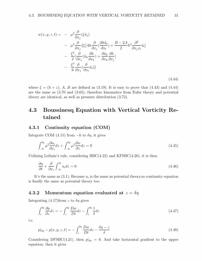
where ξ = (h + z), A, B are defined as (3.19). It is easy to prove that (4.43) and (4.44)are the same as (3.70 and (3.65), therefore kinematics from Euler theory and potentialtheory are identical, as well as pressure distribution (3.72).
4.3 Boussinesq Equation with Vertical Vorticity Re-
tained
4.3.1 Continuity equation (COM)
Integrate COM (4.15) from −h to δη, it gives
∫ δη
−hμ2∂ui
∂xidz +
∫ δη
−hμ2∂w
∂zdz = 0 (4.45)
Utilizing Leibniz’s rule, considering BBC(4.22) and KFSBC(4.20), it is then
∂η
∂t+
∂
∂xi
∫ δη
−huidz = 0 (4.46)
It’s the same as (3.1). Because ui is the same as potential theory,so continuity equationis finally the same as potential theory too.
4.3.2 Momentum equation evaluated at z = δη
Integrating (4.17)from z to δη gives
∫ δη
z
∂p
∂zdz = −
∫ δη
z
Dw
Dtdz −
∫ δη
z
1
δdz (4.47)
i.e.
p|δη − p(x, y, z, t) = −∫ δη
z
Dw
Dtdz − δη − z
δ(4.48)
Considering DFSBC(4.21), then p|δη = 0. And take horizontal gradient to the upperequation, then it gives
32CHAPTER 4. DERIVATIONS FROM EULER EQUATION WITH VERTICAL VORTICITY RETA
∇p = ∇∫ δη
z
Dw
Dtdz + ∇η
=∫ δη
z∇[
Dw
Dt]dz +
Dw
Dt|z=δηδ∇η + ∇η
(4.49)
Plug (4.49 into (4.16), then
Du
Dt+∫ δη
z∇[
Dw
Dt]dz + ∇η[δ
Dw
Dt|z=δη + 1] = 0 (4.50)
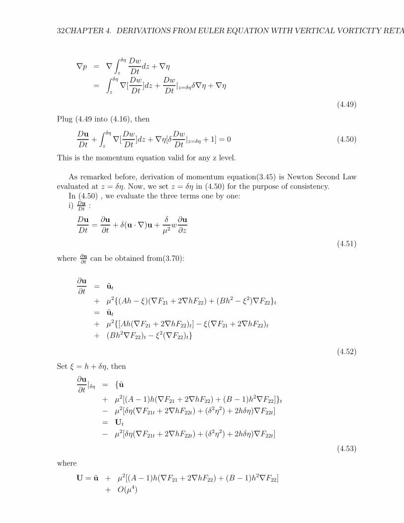
This is the momentum equation valid for any z level.
As remarked before, derivation of momentum equation(3.45) is Newton Second Lawevaluated at z = δη. Now, we set z = δη in (4.50) for the purpose of consistency.
In (4.50) , we evaluate the three terms one by one:i) Du
Dt:
Du
Dt=
∂u
∂t+ δ(u · ∇)u +
δ
μ2w
∂u
∂z
(4.51)
where ∂u∂t
can be obtained from(3.70):
∂u
∂t= ut
+ μ2{(Ah − ξ)(∇F21 + 2∇hF22) + (Bh2 − ξ2)∇F22}t
= ut
+ μ2{[Ah(∇F21 + 2∇hF22)t] − ξ(∇F21 + 2∇hF22)t
+ (Bh2∇F22)t − ξ2(∇F22)t}(4.52)
Set ξ = h + δη, then
∂u
∂t|δη = {u
+ μ2[(A − 1)h(∇F21 + 2∇hF22) + (B − 1)h2∇F22]}t
− μ2[δη(∇F21t + 2∇hF22t) + (δ2η2) + 2hδη)∇F22t]
= Ut
− μ2[δη(∇F21t + 2∇hF22t) + (δ2η2) + 2hδη)∇F22t]
(4.53)
where
U = u + μ2[(A − 1)h(∇F21 + 2∇hF22) + (B − 1)h2∇F22]
+ O(μ4)

4.3. BOUSSINESQ EQUATION WITH VERTICAL VORTICITY RETAINED 33
is the same as (3.52).The second term in (4.51) is δ(u · ∇)u, from(3.70) we have
δ(u · ∇)u = δ(u · ∇)u
+ δμ2(u · ∇)[(Ah − ξ)(∇F21
+ 2∇hF22) + (Bh2 − ξ2)∇F22]
+ δμ2([(Ah − ξ)(∇F21 + 2∇hF22) + (Bh2 − ξ2)∇F22] · ∇)u
+ O(δμ4)
= δ(u · ∇)u
+ δμ2(u · ∇[(Ah − (H + (z − δη)))(∇F21 + 2∇hF22)
+ (Bh2 − (H + (z − δη)2))∇F22]
+ δμ2{[(Ah − (H + (z − δη)))(∇F21 + 2∇hF22)
+ (Bh2 − (H + (z − δη)2))∇F22] · ∇}u(4.54)
By setting z = δη , the upper equation gives:
δ(u · ∇)u|δη = δ(u · ∇)u + δμ2(u · ∇)u1 + δμ2(u1 · ∇)u
+ δμ2u · ∇η(∇F21 + 2∇hF22 + 2H∇F22)
(4.55)
where
u1 = (Ah − H)(∇F21 + 2∇hF22) + (Bh2 − H2)∇F22 (4.56)
u1 is the second order (O(μ2)) part of u at z = δη. See equation(3.70).The third term in (4.51) is δ
μ2 w∂u∂z
. Plug (3.70)(3.71) into it,then
δ
μ2w
∂u
∂z= δμ2{(F21 + 2ξF22)(∇F21 + 2∇hF22 + 2ξ∇F22)} + O(μ4) (4.57)
By setting ξ = h + δη = H , it gives
δ
μ2w
∂u
∂z= δμ2{(F21 + 2HF22)(∇F21 + 2∇hF22 + 2H∇F22)} + O(μ4) (4.58)
ii)∫ δηz ∇[Dw
Dt]dz: This term is zero when setting z = δη, i.e.
∫ δη
z∇[
Dw
Dt]dz|z=δη = 0 (4.59)
iii)δDwDt
|z=δη :
δDw
Dt=
∂w
∂t+ δ(u · ∇)w +
δ
η2w
∂w
∂z(4.60)
where the first term is calculated by (3.71):
∂w
∂t= −μ2(F21t + 2F22tξ) (4.61)

34CHAPTER 4. DERIVATIONS FROM EULER EQUATION WITH VERTICAL VORTICITY RETA
Plug ξ = H into it, then
∂w
∂t|z=δη = −μ2(F21t + 2HF22t) (4.62)
The second term is calculated by (3.70) and (3.71)
δ(u · ∇)w = − δμ2(u · ∇)F21 − δμ22(u · ∇h)F22
− δμ22ξu · ∇F22 + O(μ4)
(4.63)
By setting ξ = H , then
δ(u · ∇)w = −δμ2u · (∇F21 + 2∇hF22 + 2H∇F22) + O(μ4) (4.64)
The third term can also be obtained from (3.71):
δ
μ2w
∂w
∂z|z=δη = δμ2(F21 + 2HF22)2F22 + O(μ4) (4.65)
Plug i) ii) and iii) into (4.50), utilizing the following identities:
(u · ∇)u1 + (u1 · ∇)u = ∇(u · u1) + (∇× u1) × u + (∇× u) × u1
(u · ∇)u =1
2∇(u · u) + (∇× u) × u
we obtain
Ut = −∇η − 1
2δ∇(u · u) + μ2Γ1 + δμ2Γ2 + Γ3 (4.66)
where
Γ1 = ∇[δηF21t + (2hδη + δ2η2)F22t] (4.67)
Γ2 = −∇{u · u1 +1
2(F21 + 2HF22)
2} (4.68)
Γ3 = − [δ(∇× u) × u + δμ2(∇× u1) × u + δμ2(∇× u) × u1
+ δμ2u · ∇δη(∇F21 + 2∇hF22 + 2H∇F22)
− δμ2∇δηu · (∇F21 + 2∇hF22 + 2H∇F22)]
(4.69)
Γ1 , Γ2 are the same as potential theory (3.53) and (3.54).Γ3 can be proved to be −δ(∇× u)|z=δη × u|z=δη, i. e.
Γ3 = −δ(∇× u)|z=δη × u|z=δη
= −δΩ|z=δη × u|z=δη
(4.70)
Comments: U is the horizontal velocity u at z = 0; Γ3 is contribution due to verticalvorticity on the surface.
4.3. BOUSSINESQ EQUATION WITH VERTICAL VORTICITY RETAINED 35
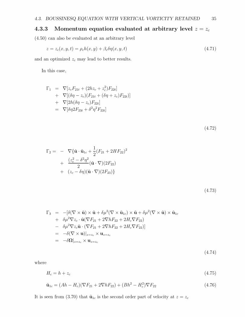
4.3.3 Momentum equation evaluated at arbitrary level z = zc
(4.50) can also be evaluated at an arbitrary level
z = zc(x, y, t) = ρch(x, y) + βcδη(x, y, t) (4.71)
and an optimized zc may lead to better results.
In this case,
Γ1 = ∇[zcF21t + (2hzc + z2c )F22t]
+ ∇[(δη − zc)(F21t + (δη + zc)F22t)]
+ ∇[2h(δη − zc)F22t]
= ∇[δη2F23t + δ2η2F22t]
(4.72)
Γ2 = − ∇{u · u1c +1
2(F21 + 2HF22)
2
+(z2
c − δ2η2
2(u · ∇)(2F22)
+ (zc − δη)(u · ∇)(2F23)}
(4.73)
Γ3 = −[δ(∇× u) × u + δμ2(∇× u1c) × u + δμ2(∇× u) × u1c
+ δμ2∇zc · u(∇F21 + 2∇hF22 + 2Hc∇F22)
− δμ2∇zcu · (∇F21 + 2∇hF22 + 2Hc∇F22)]
= −δ(∇× u)|z=zc × uz=zc
= −δΩ|z=zc × uz=zc
(4.74)
where
Hc = h + zc (4.75)
u1c = (Ah − Hc)(∇F21 + 2∇hF22) + (Bh2 − H2c )∇F22 (4.76)
It is seen from (3.70) that u1c is the second order part of velocity at z = zc

36CHAPTER 4. DERIVATIONS FROM EULER EQUATION WITH VERTICAL VORTICITY RETA
zc is free to choose, such as⎧⎪⎨⎪⎩
zc = δη on the surfacezc = 0 on the still water levelzc = −h on the bottom
The optimization of zc to get better dispersion and nonlinear properties is left for furtherinvestigation.
Comments:the result that in (4.74) we have Γ3 = −δ(∇ × u)|z=zc × uz=zc is verynatural, because the horizontal Euler equation:
∂u
∂t+ δ(u · ∇)u +
δ
μ2w
∂u
∂z= −∇p
can always be written as:
∂u
∂t+ δ
1
2∇(u · u) + δ(∇× u) × u +
δ
μ2w
∂u
∂z= −∇p
and the above equation is valid at any vertical level.One may ask : given that the kinematics between Euler theory and potential theory
are identical, why one has the vertical vorticity retained while the other does not? Theanswer is: only non-horizontal vorticity condition is used to work out the kinematics.But in potential theory, the vertical vorticity is assumed to be zero by introducing flowpotential φ. While if we rewrite the DFSBC (3.4) in such a way:
η + φt +1
2δ[∇φ · ∇φ +
1
μ2(φz)
2] = 0; z = δη (4.77)
where ∇φ is horizontal velocity u = u + u1, then as we take gradient to this equation toget momentum equation in the derivations from potential theory, we can see that
1
2∇(∇φ · ∇φ) =
1
2∇(u · u)
= (u · ∇)u− (∇× u) × u
(4.78)
where the last term gives the vorticity term accordingly. Since here u is only horizontalvelocity, doing so doesn’t harm the non-horizontal-vorticity condition in the potentialflow, but the non-vertical-vorticity condition is released.
Chapter 5
Formulations in CurvilinearCoordinates
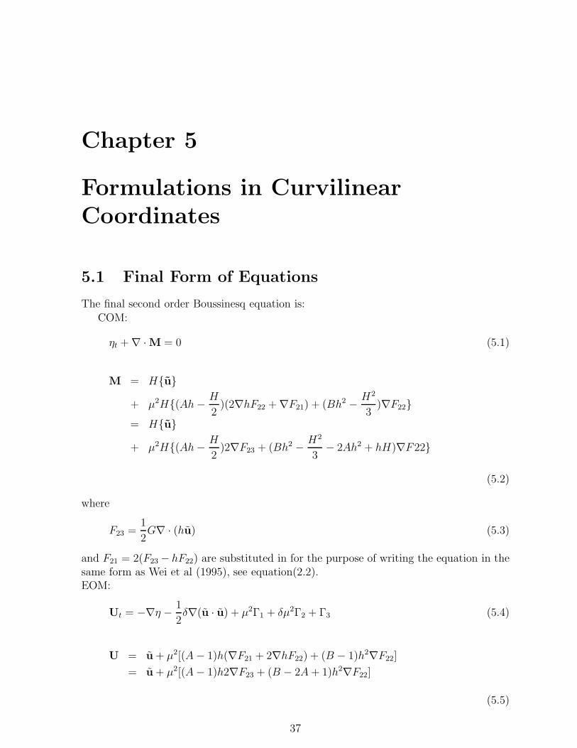
5.1 Final Form of Equations
The final second order Boussinesq equation is:COM:
ηt + ∇ · M = 0 (5.1)
M = H{u}+ μ2H{(Ah − H
2)(2∇hF22 + ∇F21) + (Bh2 − H2
3)∇F22}
= H{u}+ μ2H{(Ah − H
2)2∇F23 + (Bh2 − H2
3− 2Ah2 + hH)∇F22}
(5.2)
where
F23 =1
2G∇ · (hu) (5.3)
and F21 = 2(F23 − hF22) are substituted in for the purpose of writing the equation in thesame form as Wei et al (1995), see equation(2.2).EOM:
Ut = −∇η − 1
2δ∇(u · u) + μ2Γ1 + δμ2Γ2 + Γ3 (5.4)
U = u + μ2[(A − 1)h(∇F21 + 2∇hF22) + (B − 1)h2∇F22]
= u + μ2[(A − 1)h2∇F23 + (B − 2A + 1)h2∇F22]
(5.5)
37

38 CHAPTER 5. FORMULATIONS IN CURVILINEAR COORDINATES
Γ1 = ∇[zcF21t + (2hzc + z2c )F22t]
+ ∇[(δη − zc)(F21t + (δη + zc)F22t)]
+ ∇[2h(δη − zc)F22t]
= ∇[δη2F23t + δ2η2F22t]
(5.6)
Γ2 = − ∇{u · u1c +1
2(F21 + 2HF22)
2
+ (zc − δη)(u · ∇)(2F23)
+z2
c − δ2η2
2(u · ∇)(2F22)}
= − ∇{u · u1c +1
2(2F23 + 2δηF22)
2
+ (zc − δη)(u · ∇)(2F23)
+z2
c − δ2η2
2(u · ∇)(2F22)}
(5.7)
Γ3 = − δ(∇× u)|z=zc × uz=zc
= − δΩ|z=zc × uz=zc
= − {δ(∇× u) × u + δμ2(∇× u1c) × u + δμ2(∇× u) × u1c
+ δμ2∇zc · u(∇F21 + 2∇hF22 + 2Hc∇F22)
− δμ2∇zcu · (∇F21 + 2∇hF22 + 2Hc∇F22)}= − {δ(∇× u) × u + δμ2(∇× u1c) × u + δμ2(∇× u) × u1c
+ δμ2∇zc · u(2∇F23 + 2zc∇F22)
− δμ2∇zcu · (2∇F23 + 2zc∇F22)}
(5.8)
where
u1c = (Ah − Hc)(∇F21 + 2∇hF22) + (Bh2 − H2c )∇F22
= 2(Ah − Hc)(∇F23 + (Bh2 − H2c + 2hHc − 2Ah2)∇F22]
(5.9)
Utilizing the following identities:
(u · ∇)u1 + (u1 · ∇)u = ∇(u · u1) + (∇× u1) × u + (∇× u) × u1
5.1. FINAL FORM OF EQUATIONS 39
(u · ∇)u =1
2∇(u · u) + (∇× u) × u
we can absorb the cross products of Γ3 into 12∇(u · u) and Γ2 Then the momentum
equation(EOM) becomes:
Ut = −∇η − δ(u · ∇)u + μ2Γ1 + δμ2Γ2 + Γ3 (5.10)
and Γ2, Γ3 become:
Γ2 = − (u · ∇)u1c − (u1c · ∇)u
− ∇{1
2(2F23 + 2δηF22)
2
+ (zc − δη)(u · ∇)2F23
+z2
c − δ2η2
2(u · ∇)2F22}
(5.12)
(5.13)
Γ3 = − δμ2∇zc · u(2∇F23 + 2zc∇F22)
+ δμ2∇zcu · (2∇F23 + 2zc∇F22)
(5.14)
while Γ1 is still (5.6). The elimination of cross products in Γ3 makes the implementationa lot easier, especially for curvilinear representations.
In Chen et al (2000) version of equation, (see equation (2.20)), it’s actually represent-ing zc = zα, which leads to Bh2 = (h + zα)2 = h2
c and Ah = h + zα = Hc, then u1c = 0,so the first and the second term in the Γ2 are absent.
In dimensional formCOM:
ηt + ∇ · M = 0 (5.15)
M = H{u}+ H{(Ah − H
2)2∇F23 + (Bh2 − H2
3− 2Ah2 + hH)∇F22}
(5.16)
EOM:
Ut = −g∇η − (u · ∇)u + Γ1 + Γ2 + Γ3 (5.17)

40 CHAPTER 5. FORMULATIONS IN CURVILINEAR COORDINATES
U = u + [(A − 1)h2∇F23 + (B − 2A + 1)h2∇F22]
(5.18)
Γ1 = ∇[2ηF23t + η2F22t]
(5.19)
Γ2 = − (u · ∇)u1c − (u1c · ∇)u
− ∇{1
2(2F23 + 2ηF22)
2
+ (zc − η)(u · ∇)2F23
+z2
c − η2
2(u · ∇)2F22}
(5.21)
(5.22)
Γ3 = − ∇zc · u(2∇F23 + 2zc∇F22)
+ ∇zcu · (2∇F23 + 2zc∇F22)
(5.23)
5.2 Additional Effects for Actual Implementation
In addition to the equations shown above, we need to put the following additional effectsfor an actual implementation and from the engineering point of view:1)damping /friction2)breaking3)absorbing boundary4)subgrid mixing5)wave generation/source term6)slots for swash zone
When adding slots and source term(Tao, 1984, Kennedy et al 2000, Chen et al 2000,Wei & Kirby, 1999) the COM (5.15) becomes
b(η)ηt = E + fs(x, y, t) (5.24)
5.2. ADDITIONAL EFFECTS FOR ACTUAL IMPLEMENTATION 41
where
E = −∇ · M= −∇ · {Λ1u
+ Λ2[(Ah − h + γη
2)2∇F23
+ (Bh2 − (h + γη)2
3− 2Ah2 + h(h + γη))∇F22]}
(5.25)
b(η) =
{1, η > z∗
δ + (1 − δ)e[λ(η−z∗)/h0 ], η ≤ z∗(5.26)
where
z∗ =δh0 − h
(1 − δ)(1 − e−λ(1−h/h0))+
h0
λ− h
1 − eλ(1−h/h0)
≈ − h
1 − δ+ h0(
δ
1 − δ+
1
λ)
(5.27)
Λ1 = Λ(η), Λ2 = Λ(γη) (5.28)
where
Λ(η) =
{(η − z∗) + δ(z∗ + h0) + (1−δ)h0
λ(1 − e−λ(1+z∗/h0)), η ≥ z∗
δ(η + h0) + (1−δ)h0
λeλ(η−z∗)/h0(1 − e−λ(1+η/h0)), η ≤ z∗
(5.29)
in which h0 is a reference level lower than the lower limit of swash zone, δ is the slot widthrelative to a unit width of shoreline. Λ(η) is the total effective water depth. γ is a switchfor fully nonlinear v.s. weakly nonlinear.{
γ = 0 weakly nonlinearγ = 1 fully nonlinear
(5.30)
λ >> 1 is the shape parameter of the slots . And δ << 1. Typical values for λ and δare λ ≈ 20˜30 and δ ≈ 0.002˜0.02.
When adding damping, breaking, absorbing, source term and subgrid mixing, themomentum equation(5.17) becomes:
Ut = − g∇η − (u · ∇)u + γ(Γ1 + Γ2 + Γ3)
+ Γb + Γbr + Γsg + Γsp − g∇ps
(5.31)
Where Γb, Γbr, Γsg, Γsp and −g∇ps represent the bottom friction, breaking term, subgrid-mixing term, sponge layer term and source term respectively.
42 CHAPTER 5. FORMULATIONS IN CURVILINEAR COORDINATES
1) Damping term(friction)
Γb =−fb
h + ηu|u| (5.32)
where fb is friction coefficient. Typical value is fb ≈ 1.0 × 10⁻⁵
2) Breaking termBreaking is simulated by eddy viscosity approach which takes energy out of the main
flow.
Γbr =1
H[∇ · (ν ˜T)] (5.33)
where
˜T =1
2(∇(Hu) + ∇(Hu)T ) (5.34)
is a second order tensor represents the rate of strain.ν is eddy viscosity given by :
ν = Bbδ2b |(h + η)ηt| (5.35)
where
Bb =
⎧⎪⎨⎪⎩
1, ηt ≥ 2η∗t
ηt
η∗t− 1, η∗
t ≤ ηt ≤ 2η∗t
0, ηt ≤ η∗t
(5.36)
η∗t =
{η
(F )t , t − t0 ≥ T ∗
η(I)t + t−t0
T ∗ (η(F )t − η
(I)t ), 0 ≤ t − t0 ≤ T ∗ (5.37)
η(I)t ≈ Cbr
√gh (5.38)
η(F )t ≈ 0.15
√gh (5.39)
T ∗ ≈ 5.0√
h/g (5.40)
t0 is the time when an individual breaking event occurs. Cbr ≈ 0.3˜0.65. δb ≈ 1.0˜1.5. Theprocess is that the eddy viscosity is turned on when the acceleration ηt is greater thanη∗
t , and turned off when it drops below η∗t . The eddy viscosity given by (5.35) is filtered
before being put into Γbr in the implementation.3) Subgrid mixing termSubgrid mixing is based on Smagorinsky theory(Smagorinsky 1963)
Γsg =1
H[∇ · (νbs
˜T)] (5.41)
where
νbr = Cm�x�y| ˜D|1/2
= Cm�x�y( ˜D : ˜D)1/2
5.3. SOME NOTES ON CURVILINEAR COORDINATE 43
(5.42)
˜D =1
2[∇U + (∇U)T ] (5.43)
and U = (U, V )is short-wave averaged velocity defined in (3.77). Cm is a coefficient,typical value is about 0.2 in Funwave2D version 1.0 . �x�y represents the grid size ofthe numerical scheme, will be substituted by
√g0dξ1dξ2 where
√g0 is the Jacobian of
coordinate transform and ξ1 and ξ2 are curvilinear coordinates to be addressed later.4)Sponge layer term(Absorbing term)
Γsp = −ω1u + ω2∇ · ˜Tsp + ω3
√g/hη(e1, e2) (5.44)
where the first term represents Newton cooling, the second term represents pseudo-viscousdissipation and the third term represents sponge filter
ωi = Ciωf(x), (i = 1, 2, 3) (5.45)
for a sponge layer at down stream starts from location x = xs and ends at x = xe,f(x) is given as:
f(x) =e
x−xsxe−xs − 1
e − 1(5.46)
C1, C2, C3 are parameters to control the strength of sponge layer. ω is the frequencyof waves to be absorbed, for random wave, it’s chosen to be the peak angular frequencyof the random wave spectra.
5) Source term (wave generation)We hereby use Chawla & Kirby (2000)’s one-way wave maker theory. Detailed deriva-
tions please see appendix. The advantage of one-way wave maker is to save some gridsbehind the wave maker, otherwise we need more wave absorbing grids.
fs = D1exp(−βsx2) (5.47)
and
ps = D2xexp(−βsx2) (5.48)
where D1, D2 are defined in appendix (A.21) and (A.10), x is local Cartesian coordinatemeasured from the center of source region.
5.3 Some Notes on Curvilinear Coordinate
Before we can write the governing equation(5.24) and (5.31) in curvilinear coordinatesystem, let us define the curvilinear coordinate system first.(Shi, 2001)
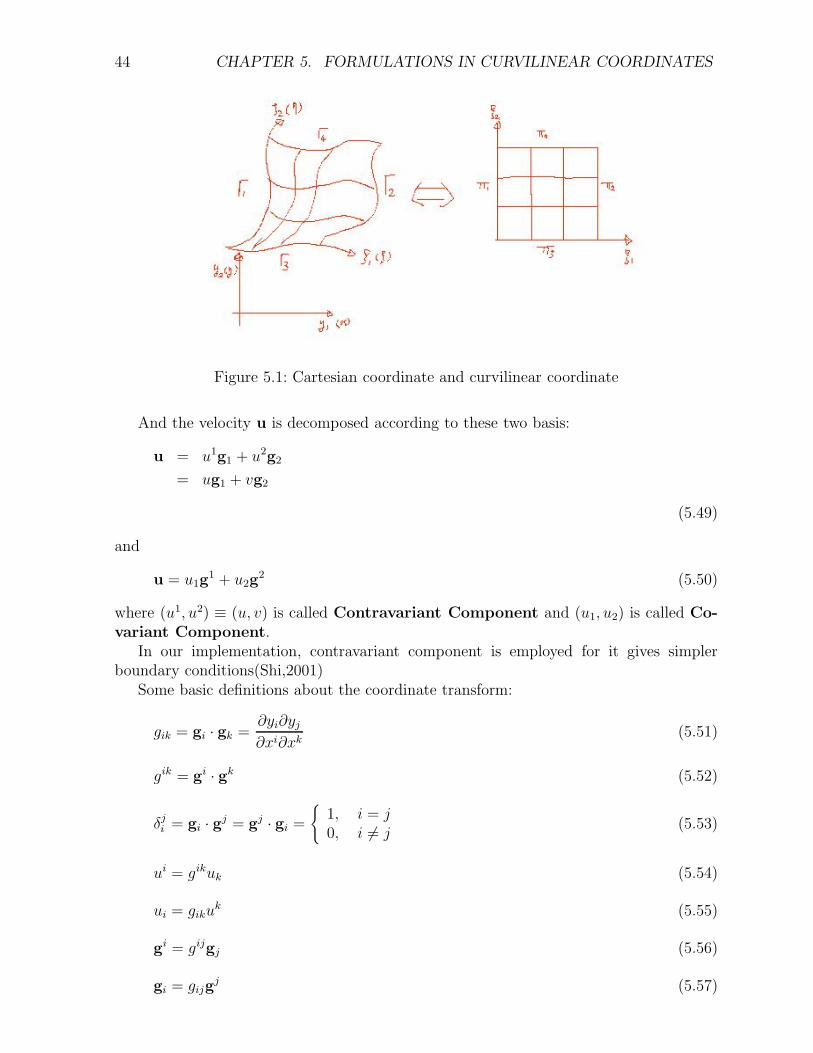
As shown in figure 5.1, the usual Cartesian coordinates (y1, y2) = (x, y) are trans-formed to curvilinear coordinates (x1, x2) = (ξ1, ξ2) = (ξ, η)
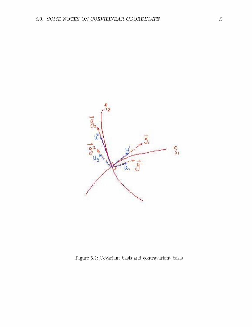
For the convenience of defining inner products and cross products, Covariant Basis(g1, g2) and Contravariant Basis (g1, g2) are defined as in figure 5.2
44 CHAPTER 5. FORMULATIONS IN CURVILINEAR COORDINATES
Figure 5.1: Cartesian coordinate and curvilinear coordinate
And the velocity u is decomposed according to these two basis:
u = u1g1 + u2g2
= ug1 + vg2
(5.49)
and
u = u1g1 + u2g
2 (5.50)
where (u1, u2) ≡ (u, v) is called Contravariant Component and (u1, u2) is called Co-variant Component.
In our implementation, contravariant component is employed for it gives simplerboundary conditions(Shi,2001)
Some basic definitions about the coordinate transform:
gik = gi · gk =∂yi∂yj
∂xi∂xk(5.51)
gik = gi · gk (5.52)
δji = gi · gj = gj · gi =
{1, i = j0, i = j
(5.53)
ui = gikuk (5.54)
ui = gikuk (5.55)
gi = gijgj (5.56)
gi = gijgj (5.57)
5.3. SOME NOTES ON CURVILINEAR COORDINATE 45
Figure 5.2: Covariant basis and contravariant basis
46 CHAPTER 5. FORMULATIONS IN CURVILINEAR COORDINATES
gikgjk = δj
i = [1 0 00 1 00 0 1
] (5.58)
√g0 = J =
∣∣∣∣∣∣∣∂y1
∂x1∂y1
∂x2∂y1
∂x3
∂y2
∂x1∂y2
∂x2∂y2
∂x3
∂y3
∂x1∂y3
∂x2∂y3
∂x3
∣∣∣∣∣∣∣ (5.59)
The last two equations give:
gij = (grsgmn − grngms)/g0 (5.60)
where⎧⎪⎨⎪⎩
i = 1 : r = 2, m = 3; j = 1 : s = 2, n = 3i = 2 : r = 2, m = 1; j = 2 : s = 3, n = 1i = 3 : r = 1, m = 2; j = 3 : s = 1, n = 2
(5.61)
Gradient, Divergence and Curl
If φ,u, ˜T represent scalar, vector, and second order tensor respectively, then
∇φ ≡ gij ∂φ
∂xjgi =
∂φ
∂xjgj ≡ φ!i (5.62)
∇ · u = ui,i =
1√g0
∂
∂xi(√
g0ui) (5.63)
∇u = uk,igkg
i (5.64)
where
uk,i =
∂uk
∂xi+ Ck
jiuj (5.65)
ui,j =
∂ui
∂xj+ Ci
kjuk (5.66)
and
Cikj =
∂2yl
∂xk∂xj
∂xi
∂yl
(5.67)
is called Christoffel Symbol of the second kind.
uk,j = gksus,j (5.68)
˜T = T ijgigj ⇒ ∇ · ˜T = T ik,k gi (5.69)
˜T = T ijgig
j ⇒ ∇ · ˜T = gjkT ij,kgi (5.70)
˜T = Tijgigj ⇒ ∇ · ˜T = gjkTij,kg
i (5.71)

5.3. SOME NOTES ON CURVILINEAR COORDINATE 47
where
T ij,k =
∂T ij
∂xk+ Ci
mkTmj + Cj
mkTim (5.72)
Tij,k =∂Tij
∂xk− Cm
ikTmj − CmjkTim (5.73)
T ij,k =
∂T ij
∂xk+ Ci
mkTmj − Cm
jkTim (5.74)
Then
T ik,k =
∂T ik
∂xk+ Ci
mkTmk + Ck
mkTim
=∂T ik
∂xk+ Ck
mkTim + Ci
mkTmk
=∂T ik
∂xk+
∂ln√
g0
∂xmT im + Ci
mkTmk
=1√g0
∂
∂xk(√
g0Tik) + Ci
mkTmk
(5.75)
Then,
∇ · ˜T = T ik,k gi
= (1√g0
∂
∂xk(√
g0Tik) + Ci
mkTmk)gi
(5.76)
∇× u =1√g0
einmum,ngi (5.77)
where einm is permutation tensor. Also we have another permutation tensor eijk given by:
gi × gj =√
g0eijkgk (5.78)
and
einmeijk = δnj δm
k − δnk δm
j (5.79)
Thus,
(∇× u) × v = (1√g0
einmum,ngi) × vjgj
=1√g0
um,nvjeinmgi × gj
=1√g0
um,nvjeinm√g0eijkgk
= um,nvj(einmeijk)gk

48 CHAPTER 5. FORMULATIONS IN CURVILINEAR COORDINATES
= um,nvj(δnj δm
k − δnk δm
j )gk
= (uk,jvj − uj,kv
j)gk
= (gksus,jv
j − gjsus,kv
j)gklgl
= (δlsu
s,jv
j − gjsgklus
,kvj)gl
= (ul,jv
j − gjsgklus
,kvj)gl
(5.80)
This equation gives the cross products in terms of contravariant components. Due to thecomplexity of this expression, we don’t use (5.8) as the form of Γ3, rather, use (5.23) inwhich the cross products are absorbed in the advection term.
Calculation of gij,√
g0, Ckij in 2-D curvilinear coordinate systems:
gik =∂yj∂yj
∂xi∂xk(5.81)
g11 = x2ξ1
+ y2ξ1
(5.82)
g22 = x2ξ2
+ y2ξ2
(5.83)
g12 = g21 = xξ1xξ2 + yξ1yξ2 (5.84)
g0 = J2 = g11g22 − g12g12 (5.85)
J = xξ1yξ2 − xξ2yξ1 =√
g0 (5.86)
g11 =g22
g0(5.87)
g22 =g11
g0
(5.88)
g12 = −g12
g0= g21 (5.89)
C111 =
1
2g11∂g11
∂ξ1+ g12∂g12
∂ξ1− 1
2g12∂g11
∂ξ2(5.90)
C211 =
1
2g12∂g11
∂ξ1+ g22∂g12
∂ξ1− 1
2g22∂g11
∂ξ2(5.91)
C222 = g12∂g12
∂ξ2− 1
2g12∂g22
∂ξ1+
1
2g22∂g22
∂ξ2(5.92)
C122 = g11∂g12
∂ξ2− 1
2g11∂g22
∂ξ1+
1
2g22∂g22
∂ξ2(5.93)
C212 = C2
21 =1
2g12∂g11
∂ξ2+
1
2g22∂g22
∂ξ1(5.94)
5.4. CURVILINEAR REPRESENTATIONS OF COM AND EOM 49
C112 = C2
21 =1
2g11∂g11
∂ξ2+
1
2g12∂g22
∂ξ1(5.95)
Relationship between Cartesian velocity (ucart, vcart) and Contravariant velocity (u1, u2) =(u, v):
ucart =Dx
Dt= u1xξ1 + u2xξ2 = uxξ1 + vxξ2 (5.96)
vcart =Dy
Dt= u1yξ1 + u2yξ2 = uyξ1 + vyξ2 (5.97)
where ∂x∂t
= 0 and ∂y∂t
= 0 are utilized for non-time-varying curvilinear coordinate system(ξ1, ξ2)
Vice versa, we have:
u = u1 =yξ2ucart − xξ2vcart√
g0(5.98)
v = u2 =xξ1vcart − yξ1ucart√
g0
(5.99)
5.4 Curvilinear Representations of COM and EOM
We chose to use contravariant velocity components u = (u1, u2).when we substitute (5.63) into COM
b(η)ηt = −∇ ·M + fs, (5.100)
it becomes
b(η)ηt = − 1√g0
∂
∂xk(√
g0Mk) + fs = E (5.101)
where (x1, x2) = (ξ1, ξ2) is curvilinear coordinate. And Mk is worked out by considering(5.62) and (5.25):
Mk = Λ1uk+ { (Ah − h + γη
2)[DHU]!k
+ (Bh2
2− Ah2 − (h + γη)2
6+
h(h + γη)
2)[DU]!k}
(5.102)
where
DHU = 2F23 = G1√g0
∂
∂xl(√
g0hul) (5.103)
DU = 2F22 = G1√g0
∂
∂xl(√
g0ul) (5.104)

50 CHAPTER 5. FORMULATIONS IN CURVILINEAR COORDINATES
k = 1, 2, and G = 11+|∇h|2 can be neglected for second order approximation. γ = 0 repre-
sents weakly nonlinear approximation and γ = 1 represents fully nonlinear approximation.Calculation of DHU and DU
DHU = G1√g0
[∂√
g0hu
∂ξ1+
∂√
g0hv
∂ξ2] (5.105)
DU = G1√g0
[∂√
g0u
∂ξ1+
∂√
g0v
∂ξ2] (5.106)
EOM:
Ut = − g∇η − (u · ∇)u + γ(Γ1 + Γ2 + Γ3)
+ Γb + Γbr + Γsg + Γsp − g∇ps
(5.107)
1) U:From (5.5),
U = u + [(A − 1)h2∇F23 + (B − 2A + 1)h2∇F22] (5.108)
then
Uk = uk + (A − 1)h[G1√g0
∂
∂xl(√
g0hul)]!k
+B − 2A + 1
2h2[G
1√g0
∂
∂xl(√
g0ul)]!k
(5.109)
The first component(k=1):
U1 = U = U − F1(v) − F2(u, v) (5.110)
where
U = u + (A − 1)hg11∂[G 1√
g0
∂∂ξ1
(√
g0hu)]
∂ξ1
+B − 2A + 1
2h2g11
∂[G 1√g0
∂∂ξ1
(√
g0u)]
∂ξ1
(5.111)
−F1(v) = + (A − 1)hg11∂[G 1√
g0
∂∂ξ2
(√
g0hv)]
∂ξ1
+B − 2A + 1
2h2g11
∂[G 1√g0
∂∂ξ2
(√
g0v)]
∂ξ1
5.4. CURVILINEAR REPRESENTATIONS OF COM AND EOM 51
(5.112)
−F2(u, v) = + (A − 1)hg21{∂[G 1√
g0
∂∂ξ1
(√
g0hu)]
∂ξ2+
∂[G 1√g0
∂∂ξ2
(√
g0hv)]
∂ξ2}
+B − 2A + 1
2h2g21{
∂[G 1√g0
∂∂ξ1
(√
g0u)]
∂ξ2+
∂[G 1√g0
∂∂ξ2
(√
g0v)]
∂ξ2}
(5.113)
The second component(k=2):
U2 = V = V − G1(u) − G2(u, v) (5.114)
where
V = v + (A − 1)hg22∂[G 1√
g0
∂∂ξ2
(√
g0hv)]
∂ξ2
+B − 2A + 1
2h2g22
∂[G 1√g0
∂∂ξ2
(√
g0v)]
∂ξ2
(5.115)
−G1(u) = + (A − 1)hg22∂[G 1√
g0
∂∂ξ1
(√
g0hu)]
∂ξ2
+B − 2A + 1
2h2g22
∂[G 1√g0
∂∂ξ1
(√
g0u)]
∂ξ2
(5.116)
−G2(u, v) = + (A − 1)hg12{∂[G 1√
g0
∂∂ξ1
(√
g0hu)]
∂ξ1+
∂[G 1√g0
∂∂ξ2
(√
g0hv)]
∂ξ1}
+B − 2A + 1
2h2g21{
∂[G 1√g0
∂∂ξ1
(√
g0u)]
∂ξ1+
∂[G 1√g0
∂∂ξ2
(√
g0v)]
∂ξ1}
(5.117)
2) pressure and first order nonlinear term−g∇η − (u · ∇)u
−g∇η − (u · ∇)u = −gη!k − uluk,l =
{F0
G0
}(5.118)
The first component(k=1):
F0 = − gη!1 − u1u1,1 − u2u1
,2
= − g[g11 ∂η
∂ξ1+ g21 ∂η
∂ξ2]
− u[∂u
∂ξ1
+ C111u + C1
21v]
− v[∂u
∂ξ2+ C1
12u + C122v]
52 CHAPTER 5. FORMULATIONS IN CURVILINEAR COORDINATES
(5.119)
The second component(k=2):
G0 = − gη!2 − u1u2,1 − u2u2
,2
= − g[g12 ∂η
∂ξ1
+ g22 ∂η
∂ξ2
]
− u[∂v
∂ξ1+ C2
11u + C221v]
− v[∂v
∂ξ2
+ C212u + C2
22v]
(5.120)
3)Γ1:
Γ1 = ∇[2ηF23t + η2F22t]
= [ηDHUT +1
2η2DUT]!k
(5.121)
where
DHUT = G1√g0
∂
∂xi(√
g0huit) (5.122)
DUT = G1√g0
∂
∂xi(√
g0uit) (5.123)
The first component(k=1):
Γ11 = F3 + F4 (5.124)
where
F3 = g11[ηDHUT +1
2η2DUT]ξ1 (5.125)
F4 = g21[ηDHUT +1
2η2DUT]ξ2 (5.126)
The second component(k=2):
Γ21 = G3 + G4 (5.127)
where
G3 = g22[ηDHUT +1
2η2DUT]ξ2 (5.128)
G4 = g12[ηDHUT +1
2η2DUT]ξ1 (5.129)
5.4. CURVILINEAR REPRESENTATIONS OF COM AND EOM 53
Calculation of DHUT and DUT:
DHUT = G1√g0
[∂√
g0hut
∂ξ1+
∂√
g0hvt
∂ξ2] (5.130)
DUT = G1√g0
[∂√
g0ut
∂ξ1
+∂√
g0vt
∂ξ2
] (5.131)
4)Γ2:
Γ2 = − (u · ∇)u1c − (u1c · ∇)u
− ∇{1
2(2F23 + 2ηF22)
2
+ (zc − η)(u · ∇)2F23
+z2
c − η2
2(u · ∇)2F22}
(5.133)
= − uluk1c,l − ul
1cuk,l
− {1
2[DHU + ηDU]2
+ (zc − η)ul ∂
∂xl(DHU)
+z2
c − η2
2ul ∂
∂xl(DU)}!k
(5.134)
The first component(k=1):
Γ12 = F5 + F6 (5.135)
where
F5 = − u1u11c,1 − u1
1cu1,1
− g11{1
2[DHU + ηDU]2
+ (zc − η)ul[∂
∂xlDHU +
zc + η
2
∂
∂xlDU]}ξ1
(5.136)
F6 = − u2u11c,2 − u2
1cu1,2
− g21{1
2[DHU + ηDU]2
+ (zc − η)ul[∂
∂xlDHU +
zc + η
2
∂
∂xlDU]}ξ2
54 CHAPTER 5. FORMULATIONS IN CURVILINEAR COORDINATES
(5.137)
where ui,j, ui
1c,j are defined in(5.66).The second component(k=2):
Γ22 = G5 + G6 (5.138)
where
G5 = − u2u21c,2 − u2
1cu2,2
− g22{1
2[DHU + ηDU]2
+ (zc − η)ul[∂
∂xlDHU +
zc + η
2
∂
∂xlDU]}ξ2
(5.139)
G6 = − u1u21c,1 − u1
1cu2,1
− g12{1
2[DHU + ηDU]2
+ (zc − η)ul[∂
∂xlDHU +
zc + η
2
∂
∂xlDU]}ξ1
(5.140)
5) Γ3:
Γ3 = − ∇zc · u(2∇F23 + 2zc∇F22)
+ ∇zcu · (2∇F23 + 2zc∇F22)
= − ∂zc
∂xjgj · uigi[(DHU)!k + zc(DU)!k]
+ z!kc uigi · [∂(DHU)
∂xj+ zc
∂(DU)
∂xj]gj
= − ∂zc
∂xjδji u
i[(DHU)!k + zc(DU)!k]
+ z!kc ui[(DHU)xj + zc(DU)xj ]δj
i
= − ∂zc
∂xjuj[(DHU)!k + zc(DU)!k]
+ z!kc uj [(DHU)xj + zc(DU)xj ]
(5.141)
The first component(k=1):
Γ13 = F7 + F8 (5.142)

5.4. CURVILINEAR REPRESENTATIONS OF COM AND EOM 55
where
F7 = − (∂zc
∂ξ1u +
∂zc
∂ξ2v)[g11∂(DHU)
∂ξ1+ g21∂(DHU)
∂ξ2
+ zc(g11∂(DU)
∂ξ1+ g21∂(DU)
∂ξ2)]
(5.143)
F8 = + (g11 ∂zc
∂ξ1+ g21 ∂zc
∂ξ2)[u
∂(DHU)
∂ξ1+ v
∂(DHU)
∂ξ2
+ zc(u∂(DU)
∂ξ1+ v
∂(DU)
∂ξ2)]
(5.144)
The second component(k=2):
Γ23 = G7 + G8 (5.145)
where
G7 = − (∂zc
∂ξ1u +
∂zc
∂ξ2v)[g12∂(DHU)
∂ξ1+ g22∂(DHU)
∂ξ2
+ zc(g12∂(DU)
∂ξ1+ g22∂(DU)
∂ξ2)]
(5.146)
G8 = + (g12 ∂zc
∂ξ1+ g22 ∂zc
∂ξ2)[u
∂(DHU)
∂ξ1+ v
∂(DHU)
∂ξ2
+ zc(u∂(DU)
∂ξ1+ v
∂(DU)
∂ξ2)]
(5.147)
6)Γb:
Γb =−fb
h + ηu|u|
=−fb
h + ηuk(u · u)1/2
=−fb
h + ηuk(umgm · ulg
l)1/2
=−fb
h + ηuk(ulul)
1/2
=−fb
h + ηuk(ulglmum)1/2
=−fb
h + ηuk[(u, v)
(g11 g12
g21 g22
)(uv
)]1/2
56 CHAPTER 5. FORMULATIONS IN CURVILINEAR COORDINATES
(5.148)
7)Γbr:
Γbr =1
H[∇ · (ν ˜T)] (5.149)
˜T =1
2(∇(Hu) + ∇(Hu)T ) (5.150)
Since
∇(Hu) = (Hui),jgigj
= gjk(Hui),jgigk (exchange j, k →)
= gkj(Hui),kgigj
,then exchange i, j in the upper equation except the basis gigj part, to get:
(∇(Hu))T = gki(Huj),kgigj. (5.151)
So,
˜T = T ijgigj =1
2[gkj(Hui),k + gki(Huj),k]gigj (5.152)
i.e.
T ij =1
2[gkj(Hui),k + gki(Huj),k] (5.153)
Thus, according to (5.76) we have:
Γbr =1
H(
1√g0
∂√
g0νT kl
∂xl+ Ck
jiνTji)gk
=
{Fbr
Gbr
}
(5.154)
The first component(k=1):
Fbr = Γ1br =
1
H[
1√g0
∂√
g0νT 11
∂ξ1+
1√g0
∂√
g0νT 12
∂ξ2
+ ν(C111T
11 + C112T
12 + C121T
21 + C122T
22)]
(5.155)
The second component(k=2):
Gbr = Γ2br =
1
H[
1√g0
∂√
g0νT 21
∂ξ1+
1√g0
∂√
g0νT 22
∂ξ2
+ ν(C211T
11 + C212T
12 + C221T
21 + C222T
22)]
(5.156)
5.4. CURVILINEAR REPRESENTATIONS OF COM AND EOM 57
8)Γsg:Since Γsg has the same structure as Γbr, it is easy to show that:
Γsg =1
H(
1√g0
∂√
g0νsgTkl
∂xl+ Ck
jiνsgTji)gk =
{Fsg
Gsg
}(5.157)
The first component(k=1):
Fsg = Γ1sg =
1
H[
1√g0
∂√
g0νsgT11
∂ξ1
+1√g0
∂√
g0νsgT12
∂ξ2
+ νsg(C111T
11 + C112T
12 + C121T
21 + C122T
22)]
(5.158)
The second component(k=2):
Gsg = Γ2sg =
1
H[
1√g0
∂√
g0νsgT21
∂ξ1+
1√g0
∂√
g0νsgT22
∂ξ2
+ νsg(C211T
11 + C212T
12 + C221T
21 + C222T
22)]
(5.159)
where
νsg = Cm√
g0dξ1dξ2(˜D : ˜D)1/2
= Cm√
g0dξ1dξ2(DijDij)
1/2
(5.160)
where
˜D =1
2[∇U + (∇U)T ] = Dijgigj = Dijg
igj (5.161)
Dij and Dij are the contravariant components and covariant components of ˜D respectively.Since
∇(U) = (Ui),jgig
j
= gjk(Ui),jgigk (exchange j, k →)
= gkj(Ui),kgigj
, then exchange i, j in the upper equation except the basis gigj to get:
(∇(U))T = gki(Uj),kgigj. (5.162)
So
Dij =1
2[gkj(U
i),k + gki(U
j),k] (5.163)
58 CHAPTER 5. FORMULATIONS IN CURVILINEAR COORDINATES
Similarly, since
∇(U) = (Ui),jgig
j (gi = gikgk →)
= gik(Ui),jg
kgj (exchange i, k →)
= gki(Uk),jg
igj
,then exchange i, j in the upper equation to get:
(∇(U))T = gkj(Uk),ig
igj. (5.164)
So
Dij =1
2[gki(U
k),j + gkj(U
k),i] (5.165)
Another way to calculate Dij is:
˜D = Dijgigj
= Dijgilglgjmgm (exchange i with l and j with m →)
= gligmjDlmgigj
= Dijgigj
thus,
Dij = gligmjDlm (5.166)
i.e., we can use the upper transform to get Dij once we calculated Dlm.Plug Dij and Dij into (5.160), then
νsg = Cm√
g0dξ1dξ2(D11D11 + D12D12 + D21D21 + D22D22)
1/2 (5.167)
9)Γsp:
Γsp = −ω1u + ω2∇ · ˜Tsp + ω3
√g/hη(e1, e2) (5.168)
where
˜Tsp = T ijspgigk (5.169)
and similar to(5.153)
T ijsp =
1
2[gkjui
,k + gkiuj,k] (5.170)
Then
Γsp = − ω1ukgk
+ ω2(1√g0
∂√
g0Tklsp
∂xl+ Ck
jiTjspi)gk
+ ω3
√g/hηek
=
{Fsp
Gsp
}

5.4. CURVILINEAR REPRESENTATIONS OF COM AND EOM 59
(5.171)
The first component(k=1):
Fsp = Γ1sp = − ω1u
+ ω2[1√g0
∂√
g0T11sp
∂ξ1+
1√g0
∂√
g0T12sp
∂ξ2
+ (C111T
11sp + C1
12T12sp + C1
21T21sp + C1
22T22sp )]
+ ω3
√g/hη
(5.172)
The second component(k=2):
Gsp = Γ2sp = − ω1v
+ ω2[1√g0
∂√
g0T21sp
∂ξ1
+1√g0
∂√
g0T22sp
∂ξ2
+ (C211T
11sp + C2
12T12sp + C2
21T21sp + C2
22T22sp )]
+ ω3
√g/hη
(5.173)
Note that ˜T, ˜D, ˜Tsp are similar in expression, so they can be calculated in a singleprocedure to save coding cost.10)∇(ps):
∇(ps) = (ps)!k
= gjk ∂ps
∂xjgk
=
{Fps
Gps
}
(5.174)
where
Fps = g11∂ps
∂ξ1+ g21∂ps
∂ξ2(5.175)
Gps = g12∂ps
∂ξ1+ g22∂ps
∂ξ2(5.176)

60 CHAPTER 5. FORMULATIONS IN CURVILINEAR COORDINATES
Figure 5.3: Shoreline boundary condition
5.5 Curvilinear Representation of Shoreline Bound-
ary Condition
As shown in figure 5.3 , at the shoreline, we require the cross boundary volume flux tobe zero.
Let M and n denote the volume flux and normal direction of the boundary respectively.Then we impose that:
M · n = 0, on ∂Ω (5.177)
where{M = M igi
n = njgj (5.178)
5.5. CURVILINEAR REPRESENTATION OF SHORELINE BOUNDARY CONDITION61
So
M · n = M igi · njgj = M injδ
ji = M ini = 0 (5.179)
i.e.
M1n1 + M2n2 = 0 (5.180)
If n = n1g1 , i.e. n2 = 0 or say ξ2 is the shoreline just like in figure 5.3, then the
upper equation gives
M1 = 0 (5.181)
Or, if n = n2g2, i.e. n1 = 0 or say ξ1 is the shoreline, then
M2 = 0 (5.182)
These two equations are very simple, that’s why we choose contravariant componentsin the implementation.
To guarantee(5.181)(5.182) to the second order of accuracy, we require(Wei & Kirby1998):
{ ∇η · n = 0u · n = 0
(5.183)
Accordingly, if n = n1g1 , then{
u1 = u = 0
(∇η)1 = η!1 = g11 ∂η∂ξ1
+ g21 ∂η∂ξ2
= 0(5.184)
and if n = n2g2, then{
u2 = v = 0
(∇η)2 = η!2 = g12 ∂η∂ξ1
+ g22 ∂η∂ξ2
= 0(5.185)
In addition, we impose
∂uT
∂n= 0 (5.186)
where uT is the tangential velocity component. This is not required physically, but canimprove the stability of numerical simulation(Wei & Kirby 1998).
i) If n = e1 = g1√g11
then as shown in figure 5.3
uT = u · e2
= uigi · g2
|g2|= uigi · g2√
g22
=uigi2√
g22
=ug12 + vg22√
g22
62 CHAPTER 5. FORMULATIONS IN CURVILINEAR COORDINATES
(5.187)
where ei and ei are unit contravariant and covariant basis.Then (please refer to Warsi 1999 book for definition of directional derivative in curvi-
linear coordinates)
∂uT
∂n= n · ∇uT
=g1
√g11
· gjk ∂uT
∂xjgk
=1√g11
gj1∂uT
∂xj
=1√g11
(uT )!1 = 0
i.e.
(uT )!1 = 0 (5.188)
ii) if n = e2 = g2√g22
then as shown in figure 5.3
uT = u · e1
= uigi · g1
|g1|= uigi · g1√
g11
=uigi1√
g11
=ug11 + vg21√
g11
(5.189)
Then
∂uT
∂n= n · ∇uT
=g2
√g22
· gjk ∂uT
∂xjgk
=1√g22
gj2∂uT
∂xj
=1√g22
(uT )!2 = 0
i.e.
(uT )!2 = 0 (5.190)
Note, that (5.188) and (5.190) are slightly different with Shi et al (2001)’s implemen-tation, where there
u2(!1) = v!1 = 0u1(!2) = u!2 =
5.5. CURVILINEAR REPRESENTATION OF SHORELINE BOUNDARY CONDITION63
0(5.191)
are used instead. The upper equations assume good orthogonality and homogeneity ofthe coordinate system (ξ1, ξ2) near the boundary, in which case g12 = g21 ≈ 0 and
√g11
and√
g22 are nearly constants so that uT ≈ v when the shoreline is on ξ2 and uT ≈ uwhen the shoreline is on ξ1. If the mesh generator is good enough, we should use (5.191)for they are much simpler.
64 CHAPTER 5. FORMULATIONS IN CURVILINEAR COORDINATES

Chapter 6
Numerics and Programming Details
The continuity equation(COM) (5.24) and momentum equation(EOM) (5.31) are solvedon image domain by Finite Difference Method using 3rd order Adams-Bashforth ex-plicit predictor and 4th order Adams-Moulton implicit corrector scheme for time integra-tion and 4th order difference scheme for O(1) part and 2nd order difference scheme forO(μ2) part for spatial discretization. Staggered grid system is employed here to improvenumerical stability. Also the boundary condition (5.177) and (5.186) are implementedin a symmetric sense rather than off-centered difference scheme in Funwave version 1.0.Numerical simulation experience shows that symmetric scheme for boundary conditionsgives better numerical stability.
6.1 Grids and Basic Spatial Difference Schemes
Figure 6.1 shows the staggered grid system. (ξ1, ξ2) = (ξ, η) is used as the coordinatecurve. ξ1 direction velocities are defined on – points(also called u points) , ξ2 directionvelocities are defined on | points(also called v points), while surface elevation and depthinformation is defined on × points(also called z points). The corner of a grid is callednode points, coordinate information is defined on node points (also called 1 points).They all use their own independent indexes.
Difference scheme for derivatives:For example ∂f
ξ|z i.e. ξ1 derivative of function f at z points (here f is defined on u
points).Second order scheme:
∂f
ξ|z =
fi+1 − fi
dξ+ O((dξ)2) (6.1)
Forth order scheme
∂f
ξ|z =
8(fi+1 − fi) − 0.5(fi+2 + fi+1) + 0.5(fi−1 + fi)
6dξ+ O((dξ)4) (6.2)
where 0.5(fi+2 + fi+1) is an average to obtain f on i + 32
point (beware that f is definedon u points) and 0.5(fi−1 + fi) is an average to obtain f on i − 1
2point. When on a
left wall boundary, fi−1 doesn’t exist, then it is replaced by fi+1 for symmetric case orreplaced by −fi+1 for anti-symmetric case. The same situation happens to fi+1 on a right
65

66 CHAPTER 6. NUMERICS AND PROGRAMMING DETAILS
Figure 6.1: Staggered grid system

6.2. FLOW CHART 67
wall boundary. For example, for ∂u∂ξ
we should use the anti-symmetric case, since u ≈ 0
at the boundary according to (5.184), an odd function satisfies this condition and it’santi-symmetric. Whereas, for ∂v
∂ξshould use the symmetric case, for ∂v
∂ξ≈ 0 according to
(5.191),an even function satisfies this and it’s symmetric.
6.2 Flow Chart
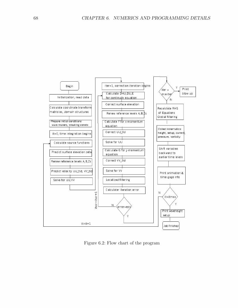
The solving procedure is: firstly, initial conditions and coordinate information as well asbathymetry information are read into memory. Then the predictor stage gives predictedvalue of surface elevation and U and V for next time step. Thereafter the corrector stageupdates the predicted values. Because the corrector scheme is implicit, the corrector stageis iterated till convergence criterion is satisfied. Since U contains u in it. It is solved by atridiagonal matrix equation to obtain u each time when U is predicted or corrected. Waveheight, setup/setdown, mean currents and other other kinematics are collected. Figure6.2 gives the flow chart.
68 CHAPTER 6. NUMERICS AND PROGRAMMING DETAILS
Figure 6.2: Flow chart of the program

6.2. FLOW CHART 69
Below is a text version:
call init
call get_gxx !Covariant matrices
call get_Cf !Christoffel symbols
call get_num_div_xy !Determine domain structures
call Wave_Maker_Preparation !Do some preparation for wave
!maker get_fs_ps
if(WaveTypeID.eq.3)call solitary_wave !Prepare the initial conditions
!for solitary wave
call breaking_parameter !Calculate some parameters for
!breaking simulation.
do it= itbegin,ntmax
call get_fs_ps !Source term in continuity and momentum
!equation for periodic/random waves
if(it=itbegin) call startup !Calculate E,F,G’s for the predictor
!using initial conditions
call predict_zeta !prediction for zeta
call get_A_B !Get reference level variables A,B
call get_Zc !Renew Zc if it’s moving with zeta
call predict_UU_tld !Predict U_tilda and V_tilda
call predict_VV_tld
call Double_sweep_UU !Solve U V
call Double_sweep_VV
do iter=1,MaxIterationNum
call slotmethod !Calculate the total volume
!of water in/out slots
call get_DHU_DU !get DHU, DU
call get_E !Calculate RHS of Continuity Eqn
call correct_zeta !correction step for zeta
call get_A_B !Get A,B’s renewed using the
!corrected water surface
call get_Zc !get Zc renewed
call get_DHUT_DUT !Calculate divergence of (h*U_t)
!and (U_t)
call get_F0~F12 !Calculate RHS of the x-momentum
!equation
call correct_UU_tld !correct UU_tilda
call Double_sweep_UU !Solve U from UU_tilda
call Sponge_Layer_UU !apply DHI sponge layer in
!x-direction (optional)
call get_DHU_DU !Renew DHU and DU
70 CHAPTER 6. NUMERICS AND PROGRAMMING DETAILS
call get_DHUT_DUT !Renew DHUT and DUT
call get_G0~G12 !Calculate RHS of the
!y-momentum equation
call correct_VV_tld !Correct VV_tilda
call Double_sweep_VV !Solve V from VV_tilda
call Sponge_Layer_VV !apply DHI sponge layer in
!y-direction (optional)
call Localized filter2D() !localized filtering for swash zone
call get_error !calculate residue of 2 successive
!iteration steps
if(error < eps) goto 100 !If converged, jump out of
!iteration cycle
if(iter.eq.MaxIterationNum)call print_blow_up
!print blow-up info.
enddo
100 call Recalculate_EFG !calculate EFG use new U,V,zeta
!for next time step
call Global Filtering !Global filtering if necessary
call Waveheight_and_Setup !collect wave height and setup
!information
call get_Umean_Vmean !collect mean currents
call get_Potential_Vorticity !Calculate Potential
!Vorticity for all points
call get_CartUV_Pressure_profile !calculate kinematics of
!gaged points.
call shift_EFG !Shift E,F12,G12, Fother,Gother backward
call print_animation !save data to animation
!files: surface,velocity,
!potential vorticity
call print_TimeGauge !search time gauge points,
!output zeta,velocity, vorticity
enddo
call print_setup_waveheight !print collected
!waveheights and setup info
End
6.3. PREDICTOR AND CORRECTOR 71
6.3 Predictor and Corrector
6.3.1 Adams explicit and implicit schemes
For a simple model equation y(t)t = f(y, t), the Adams scheme family is listed below:1)Adams 1st order explicit predictor and 2nd order implicit corrector
{yp+1 = yp + hf p
yp+1 = yi + h2(f
p+1+ f p)
(6.3)
where h is the time step, p is index current time level, p + 1 is index for next time level,
y predicted value, and fp+1
= yp+1t
2)Adams 2nd order explicit predictor and 3rd order implicit corrector
{yp+1 = yp + h
2(3f p − f p−1)
yp+1 = yi + h12
(5fp+1
+ 8f p − f p−1)(6.4)
3)Adams 3rd order explicit predictor and 4th order implicit corrector
{yp+1 = yp + h
12(23f p − 16f p−1 + 5f p−2)
yp+1 = yi + h24
(9fp+1
+ 19f p − 5f p−1 + f p−2)(6.5)
6.3.2 Implementation of Adams schemes
In our case, equation(5.101) and (5.107) are going to be solved. Since the 4th order implicitcorrector needs 3 previous levels of information, which is not available for the first 2 timesteps, so in the first step and the second step, 2nd order corrector(6.3) and 3rd corrector(6.4) are used to start up the simulation.
1)The first time step(1st order predictor, 2nd order corrector, p=1 level known)Here, p = 1 level is the initial condition obtained from inputs.Predictor(use (6.3)):
ηp+1i,j = ηp
i,j + �tEpi,j (6.6)
Up+1i,j = Up
i,j + �tF ptotal (6.7)
V p+1i,j = V p
i,j + �tGptotal (6.8)
where i, j stand for spatial indexes for ξ1 and ξ2 direction respectively,�t is time step and{Ftotal = (F12)t + Fother
Gtotal = (G12)t + Gother(6.9)
{F12 = F1 + F2
G12 = G1 + G2(6.10)
72 CHAPTER 6. NUMERICS AND PROGRAMMING DETAILS
⎧⎪⎪⎪⎨⎪⎪⎪⎩
Fother = F0 + F3 + F4 + F5 + F6 + F7 + F8
+Fb + Fbr + Fsp + Fsg − gFps
Gother = G0 + G3 + G4 + G5 + G6 + G7 + G8
+Gb + Gbr + Gsp + Gsg − gGps
(6.11)
F1, F2 and G1, G2 contain cross derivatives in U = U +F1 +F2 and V = V +G1 +G2,so they are moved to RHS of the equation. While (F12)t is approximated by
(F12)t =F p
12 − F p−112
�t(6.12)
Since, p− 1 level is not available, F p−1 is set to be same as F p as an initial guess and thistime derivative is nullified, so the upper predictor becomes actually(doing this doesn’tharm the solving procedure much, for the predictor is only a guess for the solution, andit’ll be corrected by the corrector stage, while since it might be not quite good a guessand the corrector may take more iteration steps to converge):
Up+1i,j = Up
i,j + �tF pother (6.13)
V p+1i,j = V p
i,j + �tGpother (6.14)
Corrector(use(6.3)):
ηp+1i,j = ηp
i,j +�t
2[E
p+1i,j + Ep
i,j] (6.15)
Up+1i,j = Up
i,j +�t
2[F
p+1total + F p
total] (6.16)
V p+1i,j = V p
i,j +�t
2[G
p+1total + Gp
total] (6.17)
where{F total = (F 12)t + F other
Gtotal = (G12)t + Gother(6.18)
and this time we have:
(Fp+112 )t ≈ F
p+112 − F p
12
�t(6.19)
is the same as
(Fp12)t ≈ F
p+112 − F p
12
�t(6.20)
So the upper corrector for U and V becomes:
Up+1i,j = Up
i,j + (Fp+112 − F p
12) +�t
2[F
p+1other + F p
other] (6.21)
6.3. PREDICTOR AND CORRECTOR 73
V p+1i,j = V p
i,j + (Gp+112 − Gp
12) +�t
2[G
p+1other + Gp
other] (6.22)
2)The 2nd time step(2st order predictor, 3rd order corrector, p=2)Predictor(use6.4)):
ηp+1i,j = ηp
i,j +�t
2[3Ep
i,j − Ep−1i,j ] (6.23)
Up+1i,j = Up
i,j +�t
2[3F p
total − F p−1total] (6.24)
V p+1i,j = V p
i,j +�t
2[3Gp
total − Gp−1total] (6.25)
where
(F p12)t ≈ F p
12 − F p−112
�t(6.26)
is the same as
(F p−112 )t ≈ F p
12 − F p−112
�t(6.27)
So the upper predictor for U andV becomes
Up+1i,j = Up
i,j + (F p12 − F p−1
12 )�t
2[3F p
other − F p−1other] (6.28)
V p+1i,j = V p
i,j + (Gp12 − Gp−1
12 )�t
2[3Gp
other − Gp−1other] (6.29)
Corrector(use(6.4)):
ηp+1i,j = ηp
i,j +�t
12[5E
p+1i,j + 8Ep
i,j − Ep−1i,j ] (6.30)
Up+1i,j = Up
i,j +�t
12[5F
p+1total + 8F p
total − F p−1total] (6.31)
V p+1i,j = V p
i,j +�t
12[5G
p+1total + 8Gp
total − Gp−1total] (6.32)
where
(Fp+112 )t ≈ 3F
p+112 − 4F p
12 + F p−112
2�t(6.33)
(F p12)t ≈ F
p+112 − F p−1
12
2�t(6.34)
(F p−112 )t ≈ −3F p−1
12 + 4F p12 − F
p+112
2�t(6.35)

74 CHAPTER 6. NUMERICS AND PROGRAMMING DETAILS
Then the upper corrector for U and V becomes
Up+1i,j = Up
i,j + (Fp+112 − F p
12) +�t
12[5F
p+1other + 8F p
other − F p−1other] (6.36)
V p+1i,j = V p
i,j + (Gp+112 − Gp
12) +�t
12[5G
p+1other + 8Gp
other − Gp−1other] (6.37)
3)Beyond 3rd time step(3rd order predictor, 4th order corrector, p ≥ 3)In the rest time steps we use 3rd order predictor and 4th order corrector.Predictor(use(6.5)):
ηp+1i,j = ηp
i,j +�t
12[23Ep
i,j − 16Ep−1i,j + 5Ep−2
i,j ] (6.38)
Up+1i,j = Up
i,j +�t
12[23F p
total − 16F p−1total + 5F p−2
total] (6.39)
V p+1i,j = V p
i,j +�t
12[23Gp
total − 16Gp−1total + 5Gp−2
total] (6.40)
where
(F p12)t ≈ 3F p
12 − 4F p−112 + F p−2
12
2�t(6.41)
(F p−112 )t ≈ F p
12 − F p−212
2�t(6.42)
(F p−212 )t ≈ −3F p−2
12 + 4F p−112 − F p
12
2�t(6.43)
then the upper predictor for U and V becomes
Up+1i,j = Up
i,j + (2F p12 − 3F p−1
12 + F p12) +
�t
12[23F p
other − 16F p−1other + 5F p−2
other] (6.44)
V p+1i,j = V p
i,j + (2Gp12 − 3Gp−1
12 + Gp12) +
�t
12[23Gp
other − 16Gp−1other + 5Gp−2
other] (6.45)
Corrector(use(6.5)):
ηp+1i,j = ηp
i,j +�t
24[9E
p+1i,j + 19Ep
i,j − 5Ep−1i,j + Ep−2
i,j ] (6.46)
Up+1i,j = Up
i,j +�t
24[9F
p+1total + 19F p
total − 5F p−1total + F p−2
total] (6.47)
V p+1i,j = V p
i,j +�t
24[9G
p+1total + 19Gp
total − 5Gp−1total + Gp−2
total] (6.48)
where
(Fp+112 )t ≈ 11F
p+112 − 18F p
12 + 9F p−112 − 2F p−2
12
6�t+ O(�t3) (6.49)
6.3. PREDICTOR AND CORRECTOR 75
(F p12)t ≈ 2F
p+112 + 3F p
12 − 6F p−112 + F p−2
12
6�t+ O(�t3) (6.50)
(F p−112 )t ≈ −2F p−2
12 − 3F p−112 + 6F p
12 − Fp+112
6�t+ O(�t3) (6.51)
(F p−212 )t ≈ −11F p−2
12 + 18F p−112 − 9F p
12 + 2Fp+112
6�t+ O(�t3) (6.52)
Then the upper corrector for U and V become:
Up+1i,j = Up
i,j + (Fp+112 − F p
12) +�t
24[9F
p+1other + 19F p
other − 5F p−1other + F p−2
other] (6.53)
V p+1i,j = V p
i,j + (Gp+112 − Gp
12) +�t
24[9G
p+1other + 19Gp
other − 5Gp−1other + Gp−2
other] (6.54)
6.3.3 Hot-Start problem
In the predictor stage of the first time step (6.11), we need calculate DHUT and DUTin F3, F4 and G3,G4 which are contained in Fother and Gother. But at that time, only onelevel of u and v is known from the initial condition. So we are not able to use (5.130)to calculate them. If the problem is a Cold-Start problem, i.e. the initial conditions areidentically zero. Then we can neglect these terms. While, if it’s a Hot-Start problem, wecan’t neglect them. They call for special treatments. One approach is to replace the timederivatives by spatial derivatives as follows.
From the momentum equation(5.107), we have to the O(1) order accuracy:
Ut = [u + O(μ2)]t = −g∇η + O(δ) + O(μ2) (6.55)
so,
ut = −g∇η + O(μ2) (6.56)
Then,
DUT = ∇ · ut
= −g∇ · ∇η + O(μ2)
= −g1√g0
∂
∂xi(√
g0gji ∂η
∂xj+ O(μ2)
(6.57)
Similarly,
DHUT = ∇ · (hut)
= −g∇ · (h∇η) + O(μ2)
= −g1√g0
∂
∂xi(h√
g0gji ∂η
∂xj+ O(μ2)
(6.58)
76 CHAPTER 6. NUMERICS AND PROGRAMMING DETAILS
6.4 Obtain u from U
In both the predictor and corrector stages, we get U = (U , V ), then u is obtained bysolving a tri-diagonal matrix equation.
By definition(5.111), we have
U = u + h2b1g22
g0
[1√g0
(√
g0u)ξ1 ]ξ1
+ hb2g22
g0[
1√g0
(√
g0hu)ξ1 ]ξ1
(6.59)
where
b1 =B − 2A + 1
2(6.60)
and
b2 =B − 2A + 1
2(6.61)
(6.59) is a second order differential equation for u, and we can solve it by a tri-diagonalmatrix system. Since A, B are related to definitions of the multiple and moving referencelevel, it’s a function of time. So the coefficients of the equation are time varying.
For a given u point i, the upper equation can be discretized as:
AAiui−1 + ui + CCiui+1 = DDi (6.62)
where
AAi = (√
g0)i−1(hg22
g20
)i[hib1(√
g0)i + hi−1b2(√
g0)i
+ (1
2hib1 +
1
2hi−1b2)(
√g0)ξ1]/BB
CCi = (√
g0)i+1(hg22
g20
)i[hib1(√
g0)i + hi+1b2(√
g0)i
− (1
2hib1 +
1
2hi+1b2)(
√g0)ξ1]/BB
DDi = Ui (6.63)
BB = 1 − 2(h2g22
g0)i(b1 + b2) (6.64)
If i is on a wall boundary, then i − 1 in AAi is replaced by i + 1 when the wall is atleft; and i + 1 in CCi is replaced by i − 1 when the wall is at right. (6.62) is a standardtri-diagonal matrix system, can be readily solved. v can be solved in the same way.

6.5. ITERATION ERROR CONTROL AND UNDER-RELAXATION 77
6.5 Iteration Error Control and Under-relaxation
Between iteration step k and k+1 , the errors of iteration are defined as:
errorz =
∑i
∑j |ηk+1
i,j − ηki,j|∑
i
∑j |ηk+1
i,j | (6.65)
erroruv =
∑i
∑j |uk+1
i,j − uki,j| + |vk+1
i,j − vki,j|∑
i
∑j |uk+1
i,j | + |vk+1i,j | (6.66)
while in the very first few time steps, the denominator may be very small for a cold-start problem, in that case, if the denominator is less than 1.0E − 6 the upper errors aredefined as the numerator to avoid devision by a small number.
The convergence criteria is when max(erroruv, errorz) is less than an designatedvalue,then the iteration stops.
Also, an under-relaxation method is applied to get better numerical stability. It isdesigned as:
(u, v, η) = ω(u, v, η)k+1 + (1 − ω)(u, v, η)k (6.67)
where ω is relaxation parameter chosen to be between 0.5 ˜1.0 .
6.6 Calculation of Kinematics
In light of the kinematics formulas (3.73) ˜(3.81), they are calculated in the code.Horizontal velocity:From (3.73)
u(ξ1, ξ2, z, t) = u + (Ah − (h + z))∇∇ · (hu)
+ (B − 2A
2h2 − (h + z)2
2+ h(h + z))∇∇ · u
= u + (Ah − (h + z))(DHU)!i
+ (B − 2A
2h2 − (h + z)2
2+ h(h + z))(DU)!i
= (u, v)
(6.68)
Here u, v are contravariant components in the image domain, for convenience of engineer-ing usage, they are converted to Cartesian components by (5.96) and (5.97).
Vertical velocity:From(3.74),we can obtain
w(x, y, z, t) = −(DHU + zDU) (6.69)
and it’s a linear function of z as a second order model.Pressure:
78 CHAPTER 6. NUMERICS AND PROGRAMMING DETAILS
From(3.75), we can obtain:
p(x, y, z, t) = pa + ρg(η − z)
− ρ{(η − z)DHUT + [((h + η)2 − (h + z)2)
2− h(η − z)]DUT
+ u · [(η − z)∇DHU
+ (((h + η)2 − (h + z)2)
2− h(η − z))∇DU]}
(6.70)
Mean Current:Mean current is calculated by
(U, V ) = (M1
h + η,
M2
h + η) (6.71)
and then converted to Cartesian coordinate by (5.96) and (5.97).Potential Vorticity:Potential Vorticity is calculated by(3.78):
q(x, y, t) =1√g0
[∂(g21(
M1
h+η) + g22(
M2
h+η)
∂ξ
− ∂(g11(M1
h+η) + g12(
M2
h+η)
∂η]/(h + η)
(6.72)

Appendix A
Wave Maker Theory
The wave maker mechanism here is basically adding a periodic forcing term to the equa-tion. FUNWAVE 1.0 uses a two-way wave maker where a forcing term symmetric aboutthe central line of source region is added to the continuity equation. Theory has beendeveloped by Wei et al(1999), basically using Fourier Transform method to solve thelinearized equation to obtain the transfer function between the desired wave height andsource strength. Chawla & Kirby (2000) developed a one-way wave maker by furtheradding a forcing term anti-symmetric about the central line of source region, and Dopplereffects of background current is also taken into account. Here the derivation of Chawla &Kirby (2000) is repeated for the linearized version of Boussinesq Equation, but no Dopplereffect is considered for simplicity.
The 1D linearized version of Boussinesq Equation(5.1)(5.4) with constant depth h is:COM:
ηt + h∇ · u + μ2α1h3∇2(∇ · u) = 0 (A.1)
EOM:
ut + ∇η + μ2αh2∇(∇ · ut) = 0 (A.2)
where α = B−12
, α1 = α+1/3 = B/2−1/6. Since h is constant and equation is linearized,here B is also a constant, means that the moving part in B has been taken out, hence αand α1 are constant too. zc in (4.71) is also set to be constant for linea rization and finallydisappears here. The upper two equations are of the same form of Chawla & Kirby(2000)equation (4a) and (4b), except that the current U there is now set to be zero and thedefinition of α is different. So all the derivations in Chawla & Kirby (2000) hold at here.
When introducing source functions in both continuity and momentum equations, weget(in dimensional form):COM:
ηt + h∇ · u + α1h3∇2(∇ · u) = fs(x, y, t) (A.3)
EOM:
ut + g∇η + αh2∇(∇ · ut) = −g∇ps(x, y, t) (A.4)
where fs and ps can be rewritten as follows by introducing Fourier Transform in time andspanwise direction:
fs(x, y, t) =1
4π2
∫ ∞
−∞
∫ ∞
−∞fs(x, λ, ω)ei(λy−ωt)dλdω (A.5)
79
80 APPENDIX A. WAVE MAKER THEORY
ps(x, y, t) =1
4π2
∫ ∞
−∞
∫ ∞
−∞ps(x, λ, ω)ei(λy−ωt)dλdω (A.6)
where fs and ps are transfer function of fs and ps respectively. By following Chawla &Kirby(2000) derivations, we obtain:
fs = D1e−βsx2
(A.7)
ps = D2xe−βsx2
(A.8)
where
D1 =−iη0e
(l21
4βs)
a1
√πβs
(2ω)(1 − αh2k2)(A.9)
and
D2 =−2βsD1
l1ω(A.10)
βs =80
γ2rL
2(A.11)
where η0 is the desired wave amplitude , ω is the angular frequency of a single wavecomponent, L is typical wave length, γr is a parameter to control the source region widthW :
W = γrL
2(A.12)
.a1 is given as
a1 =i
As(l1 − l2)(l1 + l2)2l1(A.13)
where
l1 = (Cs −
√C2
s − 4AsEs
2As
)1/2 (A.14)
l2 = (Cs +
√C2
s − 4AsEs
2As
)1/2 (A.15)
and l21 + λ2 = k2, here l1 = k cos θ and λ = k sin θ, where θ is the wave direction and k isthe wavenumber given by dispersion relationship:
ω2 = ghk21 − α1k2h2
1 − αk2h2(A.16)
As, Cs, Es are given as:
As = α1gh3 (A.17)
81
Cs = gh + ω2αh2 − 2α1λ2gh3 (A.18)
Es = ω2[1 − α(λh)2] − ghλ2[1 − α1(λh)2] (A.19)
By using the dispersion relation, a1 can be simplified to:
a1 =−ik
2(ω2 − α1gh3k4) cos θ(A.20)
then D1 can be written as:
D1(η0, ω, θ) =η0 cos θe(
l214βs
)ω2 − α1gh3k4)
ωk√
πβs
(1 − αh2k2)(A.21)
Then the source function fs(x, y, t) is calculated by Discrete Fourier Transform fordirectional waves:
fs(x, y, t) = Real{ 1
4π2
∫ ∞
−∞
∫ ∞
−∞fs(x, λ, ω)ei(λy−ωt)dλdω}
=M∑i=1
N∑j=1
fs(x, λj , ωi, η0ij)[ei(λjy−ωit+φ0) + c.c.]
1
2
=M∑i=1
N∑j=1
fs(x, λj , ωi, η0ij) cos(λjy − ωit + φ0)
(A.22)
where φ0 is a random phase given from 0 to 2π, η0ij is the wave amplitude for the i’thfrequency component and the j’th directional component given by selected power densityspectrum:
η0ij = η0(ωi, θj)
=√
2S(ωi)G(θj)dωidθj
=√
2S(ωi)dωi ( if only frequency spectrum exists)
=√
2G(θj)dθj ( if only directional spectrum exists)
(A.23)
where S(ωi) , G(θj) are power density spectrum.ps(x, y, t) is calculated in the same way:
ps(x, y, t) =M∑i=1
N∑j=1
ps(x, λj , ωi, η0ij) cos(λjy − ωit + φ0) (A.24)

82 APPENDIX A. WAVE MAKER THEORY

Appendix B
Mesh Generator by Fengyan Shi
The program needs preprocessor to prepare bathymetry and grid type data files. Thiscan be done using CoastGrid program developed by Dr. Fengyan Shi in CACR. For de-tails please go to http://coastal.udel.edu/ fyshi/coastgrid/coastgrid.html . The CoastGridprogram enables us to generate generalized meshes fitted with boundary and output gridpoints. For the grid type data, Funwave2D can’t tolerate structures/islands and waterdomains that are about one grid wide in any direction, otherwise, ambiguity of gridtypedefinition will occur. If this happens in your mesh, you need to refine the mesh locally toavoid it.
A Fortran program gridtype.f is also included to generate grid type files using bathymetrydata as input.
83

84 APPENDIX B. MESH GENERATOR BY FENGYAN SHI
Bibliography
[1] Berkhoff, J. C. W., Booy, N. and Radder, A. C.,, Verification of numerical wavepropagation models for simple harmonic linear water waves, Coastal Engrg, 6, pp255-279, 1982
[2] Chawla, A. and Kirby, J. T., A source function method for generation of waves oncurrents in Boussinesq models, Applied Ocean Research, V22, 75-83, 2000
[3] Chen, Q., Kirby, J. T., Dalrymple, R. A., Kennedy, A. B. and Chawla, A., Boussinesqmodeling of wave transformation, breaking and runup. II: Two horizontal dimensions,Journal of Waterway, Port, Coastal and Ocean Engineering, 126, 48-56, 2000.
[4] Gobbi, M. F., Kirby, J. T. and Wei, G., A fully nonlinear Boussinesq model for surfacewaves. II. Extension to O(kh4), Journal of Fluid Mechanics, 405, 181-210, 2000.
[5] Gobbi, M. F. and Kirby, J. T., Wave evolution over submerged sills: Tests of a high-order Boussinesq model, Coastal Engineering, 37, 57-96, 1999, and erratum, 40, 277,2000.
[6] Kennedy, A. B, Chen, Q., Kirby, J. T., and Dalrymple, R. A., Boussinesq modeling ofwave transformation, breaking and runup. I: One dimension, Journal of Waterway,Port, Coastal and Ocean Engineering, 126, 39-47, 2000.
[7] Kennedy, A. B., Kirby, J. T., Chen, Q. and Dalrymple, R. A., Boussinesq-type equa-tions with improved nonlinear behaviour, Wave Motion, 33, 225-243, 2001.
[8] Kirby, J. T., Boussinesq models and applications to nearshore wave propagation,surfzone processes and wave-induced currents, Advances in Coastal Engineering, V.C. Lakhan(ed), Elsevier, 2003
[9] Mase, H. and Kirby, J. T., Modified frequency domain KdV equation for randomwave shoaling, Proc. 23d Intl. Conf. Coastal Engrng, Venice, 474-487, October 1992.
[10] Nwogu, O., An alternative form of the Boussinesq equations for nearshore wave prop-agation, J. Waterway, Port, Coast., Ocean Engrg, 119(6), 618-638, 1993
[11] Shi, F., Dalrymple, R. A., Kirby, J. T., Chen, Q. and Kennedy, A., A fully nonlinearBoussinesq model in generalized curvilinear coordinates, Coastal Engineering, 42,337-358, 2001.
[12] Smagorinsky, J.S., 1963, General circulation experiments with the primitive equa-tions, Mon. Weather Rev. V93, pp99- .
85
86 BIBLIOGRAPHY
[13] Tao, J., Computation of wave run-up and wave breaking Internal report, DanishHydraulic Institute, 1983
[14] Tao, J., Numerical modeling of wave runup and breaking on the beach ActaOceanologica Sinica, 6(5), pp692-700, in Chinese, 1984.
[15] Warsi, Z.U.A. Fluid Dynamics. Theoretical and Computational Approaches.2. BocaRaton CRC 1999
[16] Watanabe, A., Maruyama, K., Numerical modeling of nearshore wave field undercombined refraction, diffraction and breaking, Coastal Engineering in Japan, V29,1986
[17] Wei, G., Kirby, J. T., Grilli, S. T. and Subramanya, R., A fully nonlinear Boussi-nesq model for surface waves. I. Highly nonlinear, unsteady waves, Journal of FluidMechanics, 294, 71-92, 1995.
[18] Wei, G., Kirby, J. T. and Sinha, A., Generation of waves in Boussinesq models usinga source function method, Coastal Engineering, 36, 271-299, 1999.
[19] Wei,G., Kirby, J.T., Simulation of water waves by Boussinesq models, Research Re-port No. CACR-98-02, Center for Applied Coastal Research, University of Delaware,Newark, Delaware.