機械学習を用いた予測モデル構築・評価
DESCRIPTION
TRANSCRIPT

機械学習を用いた予測モデルの構築・評価
2014年4月19日
第38回Tokyo.R
@sfchaos
自己紹介
TwitterID: @sfchaos
お仕事: 人工知能的な何か
(データマイニング,
セマンティックWeb, オントロジー, etc.)
1
RDFOWL
SPARQL

自己紹介
TwitterID: @sfchaos
お仕事: 人工知能的な何か
(データマイニング,
セマンティックWeb, オントロジー, etc.)
2
DFOWL(アール〔アウル〕と読むっぽい)
SPA QL

アジェンダ
1. イントロダクション
2. 予測モデル構築・評価の考え方
3. 予測モデル構築・評価 基礎編
4. 予測モデル構築・評価 発展編
5. まとめ
3

1. イントロダクション
4

はじめての予測モデル
5
アヤメの種類を予測するモデルが欲しいのよ.明日の朝までに至急作ってちょうだい.
データがこうスッと来たらバァッといってガーンと作ればできるでしょ?

更け行く夜・・・
6
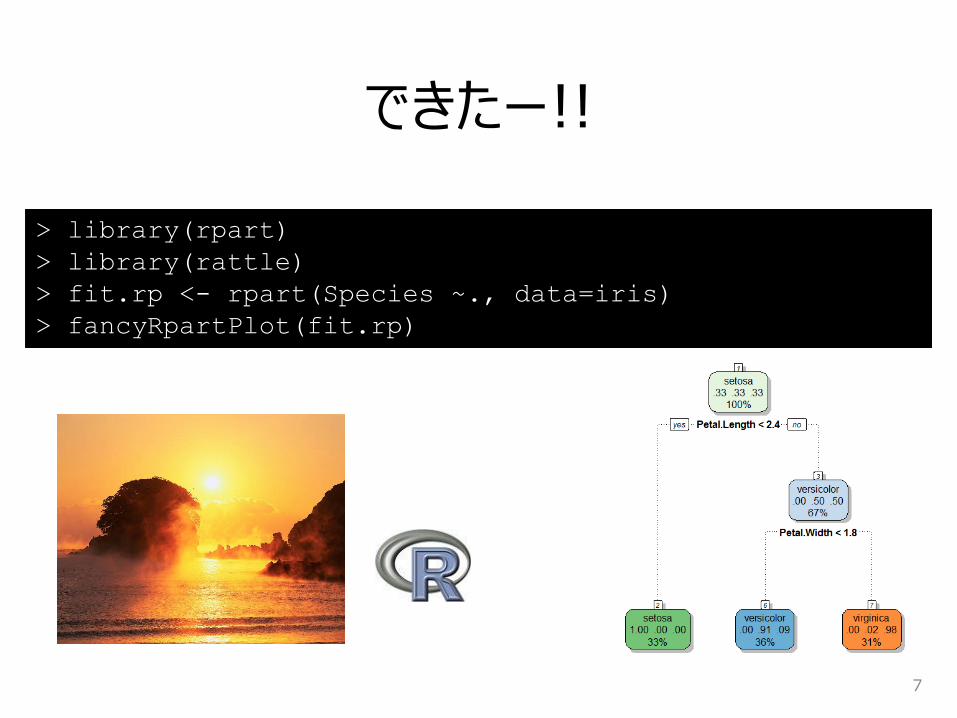
できたー!!
7
> library(rpart)
> library(rattle)
> fit.rp <- rpart(Species ~., data=iris)
> fancyRpartPlot(fit.rp)

数日後・・・
8
明日の朝までに至急作り直してちょうだい
あんたが作った予測モデル全然あたらないじゃないのよ!
☆◎×??
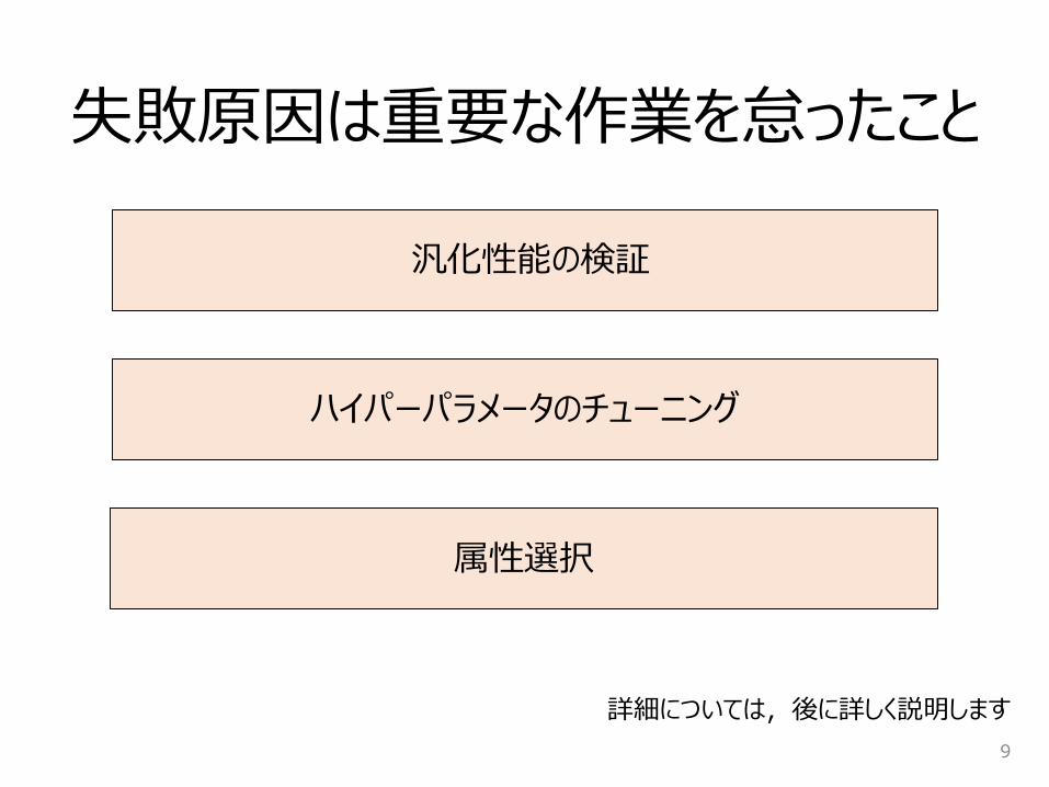
失敗原因は重要な作業を怠ったこと
汎化性能の検証
9
ハイパーパラメータのチューニング
属性選択
詳細については,後に詳しく説明します

またしても更け行く夜・・・
10
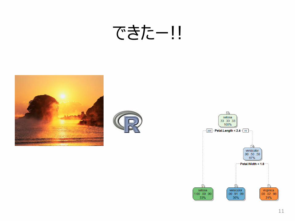
できたー!!
11

さらに数日後・・・
12
そういえば,世の中にはいろんな機械学習の
アルゴリズムがあるらしいわね.
全部やってちょうだい.
精度はまあまあ出るようにはなってきたわ.でも・・・何かが足りないわ.

It’s very hard…
13
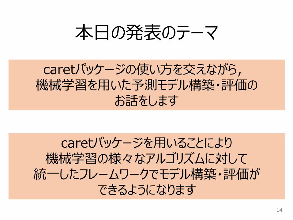
本日の発表のテーマ
14
caretパッケージの使い方を交えながら,機械学習を用いた予測モデル構築・評価の
お話をします
caretパッケージを用いることにより機械学習の様々なアルゴリズムに対して
統一したフレームワークでモデル構築・評価ができるようになります

2. 予測モデル構築・評価の考え方
15
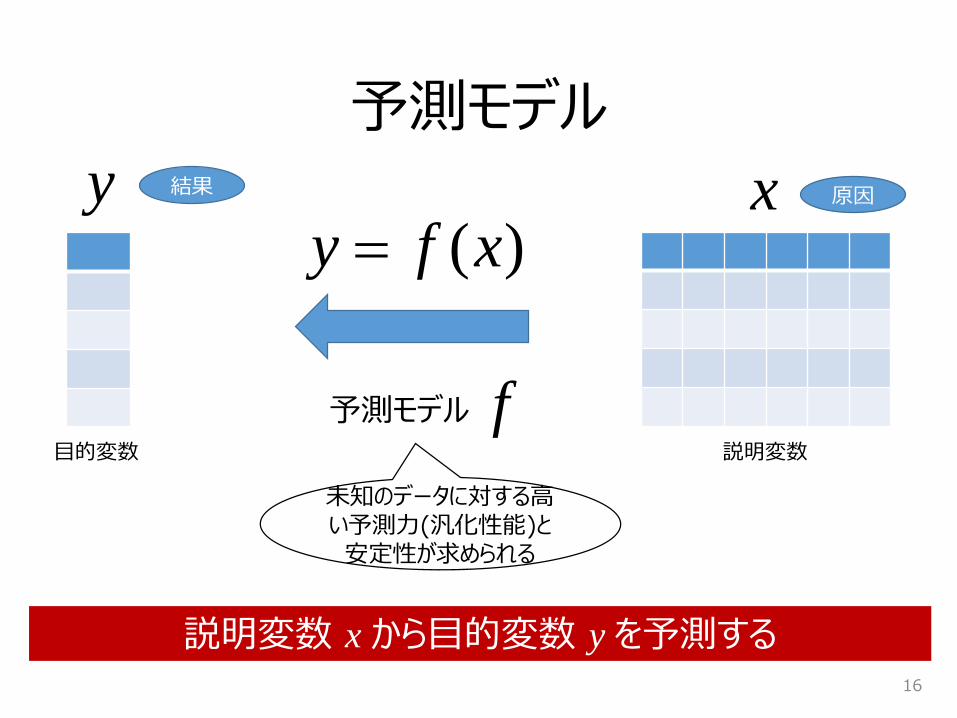
予測モデル
16
目的変数 説明変数
xy)(xfy
予測モデル f
説明変数 x から目的変数 y を予測する
結果 原因
未知のデータに対する高い予測力(汎化性能)と安定性が求められる
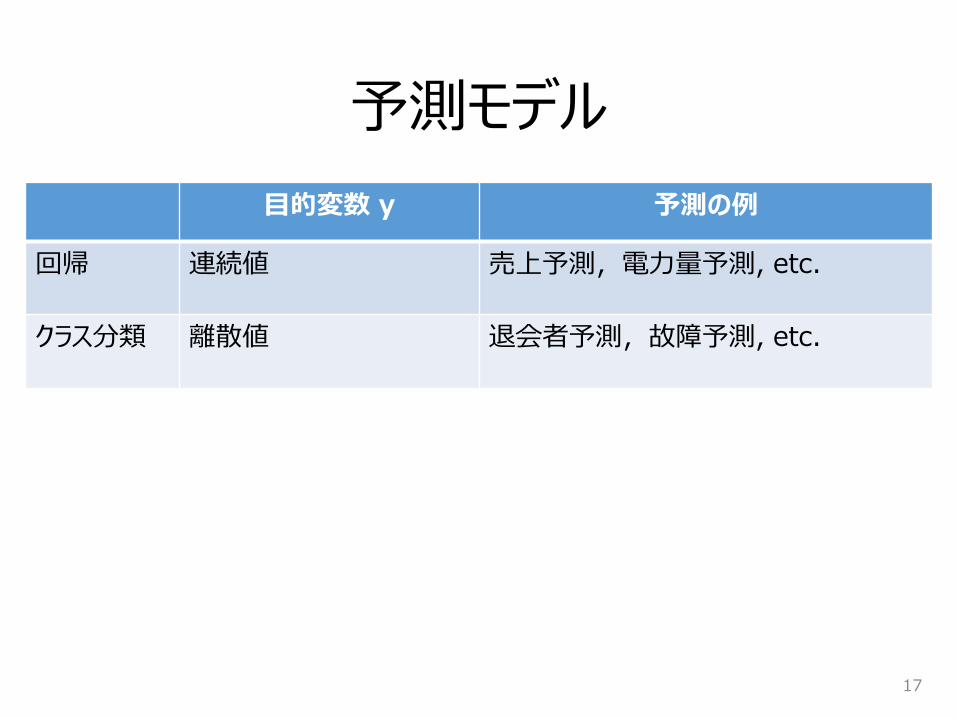
予測モデル
17
目的変数 y 予測の例
回帰 連続値 売上予測,電力量予測, etc.
クラス分類 離散値 退会者予測,故障予測, etc.
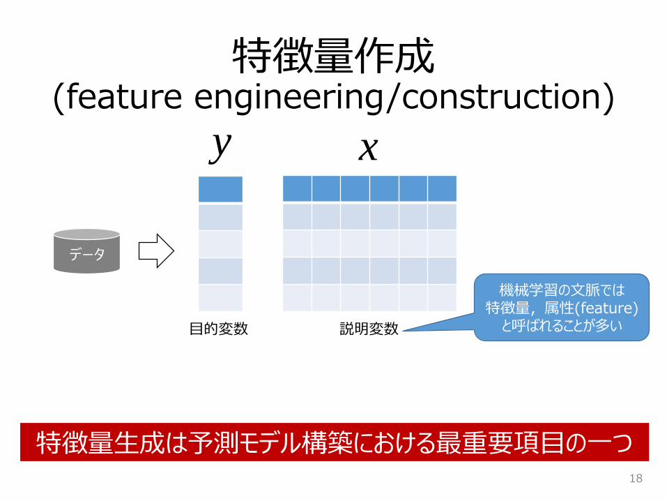
特徴量作成(feature engineering/construction)
18
データ
目的変数 説明変数
機械学習の文脈では特徴量,属性(feature)
と呼ばれることが多い
xy
特徴量生成は予測モデル構築における最重要項目の一つ
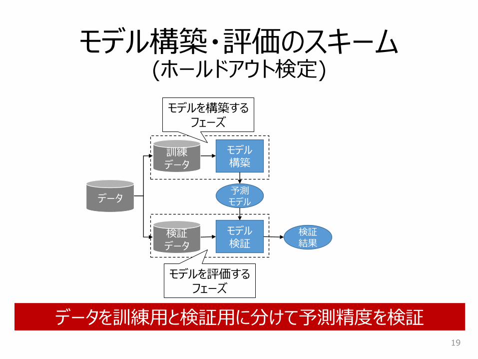
モデル構築・評価のスキーム(ホールドアウト検定)
19
データ
訓練データ
検証データ
モデル構築
予測モデル
モデル検証
検証結果
モデルを評価するフェーズ
データを訓練用と検証用に分けて予測精度を検証
モデルを構築するフェーズ
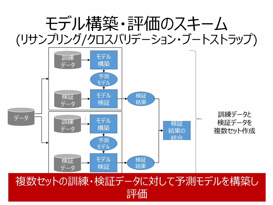
モデル構築・評価のスキーム(リサンプリング/クロスバリデーション・ブートストラップ)
20
データ
訓練データ
検証データ
モデル構築
予測モデル
モデル検証
検証結果
訓練データ
検証データ
モデル構築
予測モデル
モデル検証
検証結果
・・・
訓練データと検証データを
複数セット作成検証
結果の統合
複数セットの訓練・検証データに対して予測モデルを構築し評価
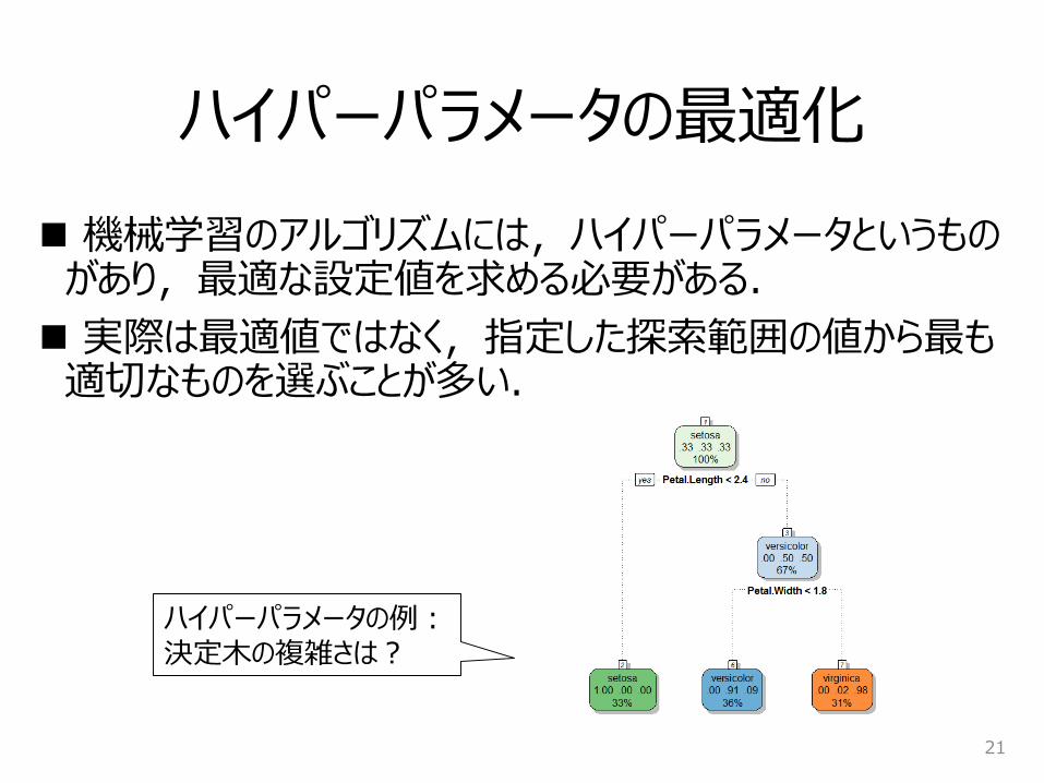
ハイパーパラメータの最適化
機械学習のアルゴリズムには,ハイパーパラメータというものがあり,最適な設定値を求める必要がある.
実際は最適値ではなく,指定した探索範囲の値から最も適切なものを選ぶことが多い.
21
ハイパーパラメータの例:決定木の複雑さは?
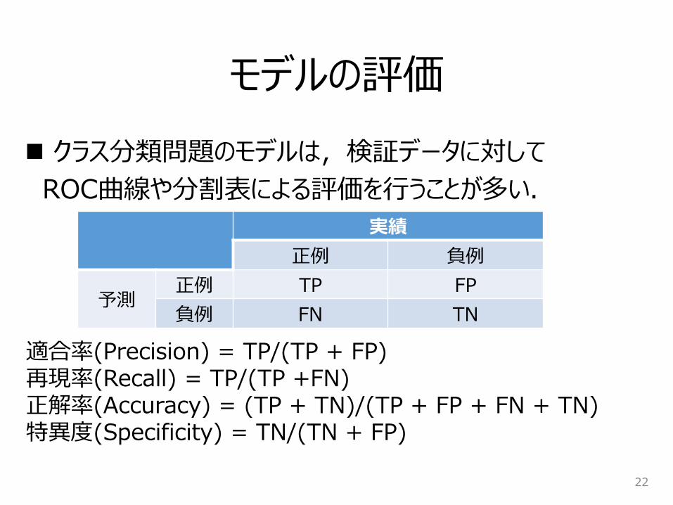
モデルの評価
22
適合率(Precision) = TP/(TP + FP)再現率(Recall) = TP/(TP +FN)正解率(Accuracy) = (TP + TN)/(TP + FP + FN + TN)特異度(Specificity) = TN/(TN + FP)
クラス分類問題のモデルは,検証データに対して
ROC曲線や分割表による評価を行うことが多い.
実績
正例 負例
予測正例 TP FP
負例 FN TN
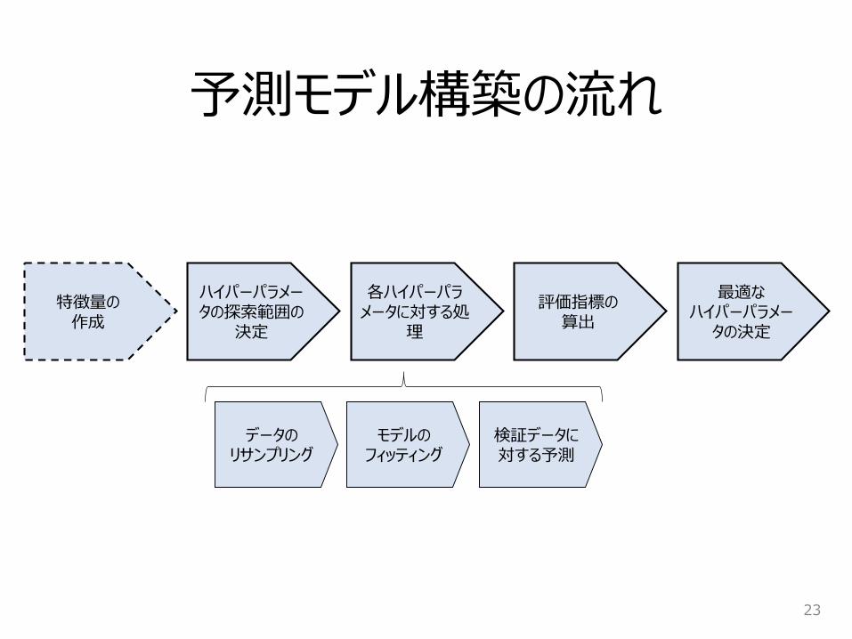
予測モデル構築の流れ
23
ハイパーパラメータの探索範囲の
決定
各ハイパーパラメータに対する処
理
評価指標の算出
最適なハイパーパラメー
タの決定
データのリサンプリング
モデルのフィッティング
検証データに対する予測
特徴量の作成

3. 予測モデル構築・評価 基礎編
24
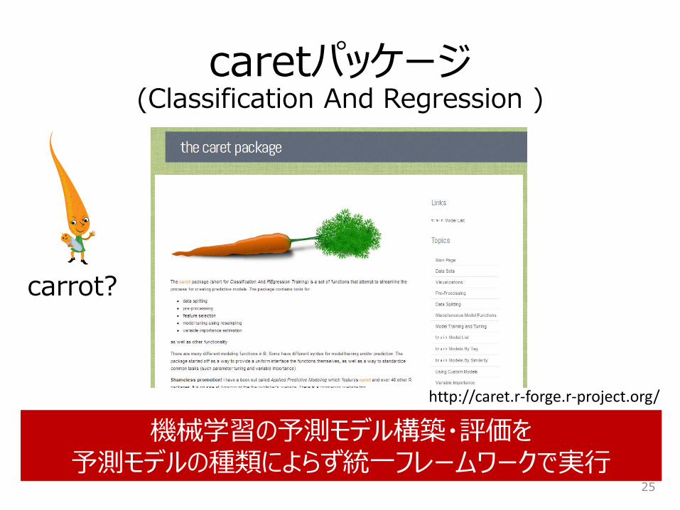
caretパッケージ(Classification And Regression )
25
http://caret.r-forge.r-project.org/
機械学習の予測モデル構築・評価を予測モデルの種類によらず統一フレームワークで実行
carrot?

作者はPfizerのデータ分析者
Max Kuhn氏
26
http://www.predictiveanalyticsworld.com/boston/2012/speakers.php
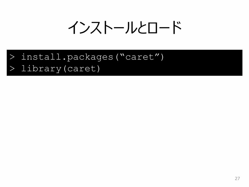
インストールとロード
27
> install.packages(“caret”)
> library(caret)
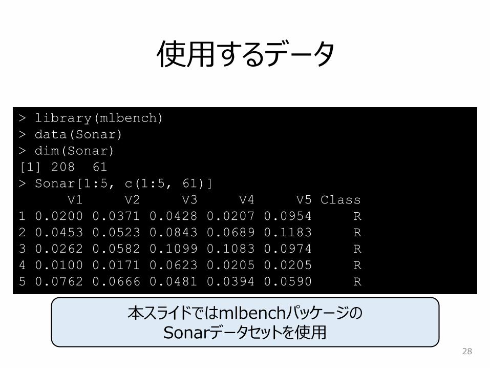
> library(mlbench)
> data(Sonar)
> dim(Sonar)
[1] 208 61
> Sonar[1:5, c(1:5, 61)]
V1 V2 V3 V4 V5 Class
1 0.0200 0.0371 0.0428 0.0207 0.0954 R
2 0.0453 0.0523 0.0843 0.0689 0.1183 R
3 0.0262 0.0582 0.1099 0.1083 0.0974 R
4 0.0100 0.0171 0.0623 0.0205 0.0205 R
5 0.0762 0.0666 0.0481 0.0394 0.0590 R
使用するデータ
28
本スライドではmlbenchパッケージのSonarデータセットを使用
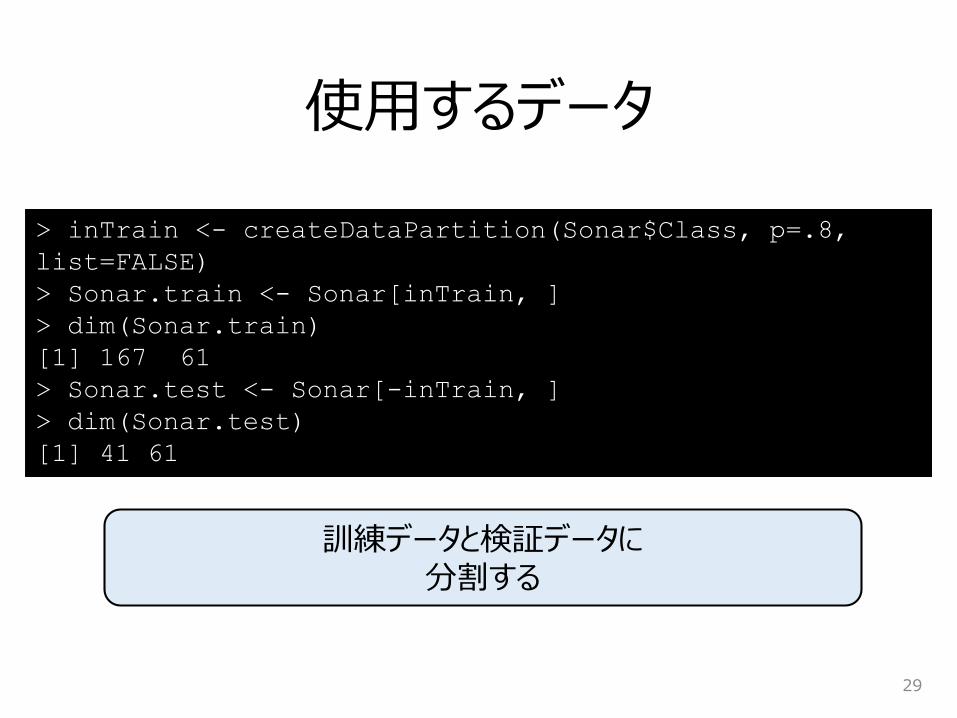
> inTrain <- createDataPartition(Sonar$Class, p=.8,
list=FALSE)
> Sonar.train <- Sonar[inTrain, ]
> dim(Sonar.train)
[1] 167 61
> Sonar.test <- Sonar[-inTrain, ]
> dim(Sonar.test)
[1] 41 61
使用するデータ
29
訓練データと検証データに分割する
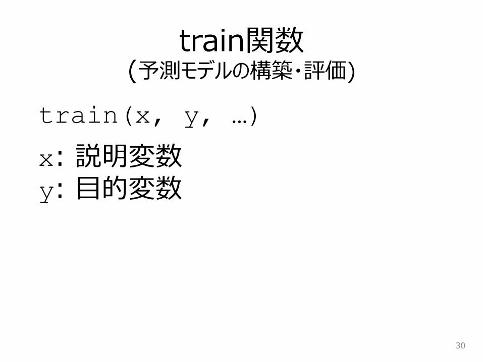
train関数(予測モデルの構築・評価)
30
train(x, y, …)
x: 説明変数y: 目的変数
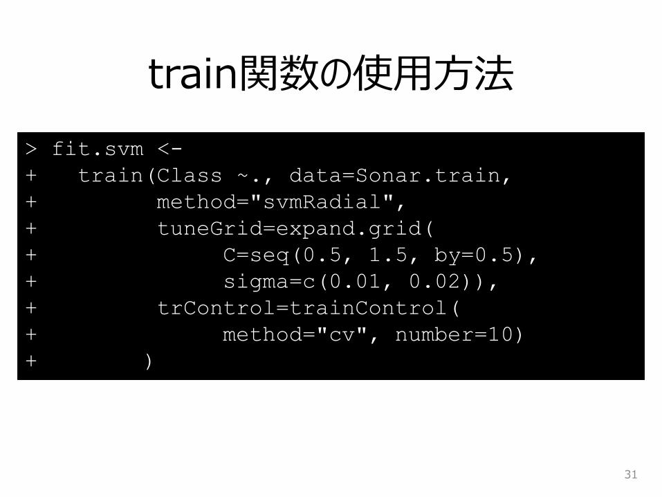
train関数の使用方法
31
> fit.svm <-
+ train(Class ~., data=Sonar.train,
+ method="svmRadial",
+ tuneGrid=expand.grid(
+ C=seq(0.5, 1.5, by=0.5),
+ sigma=c(0.01, 0.02)),
+ trControl=trainControl(
+ method="cv", number=10)
+ )
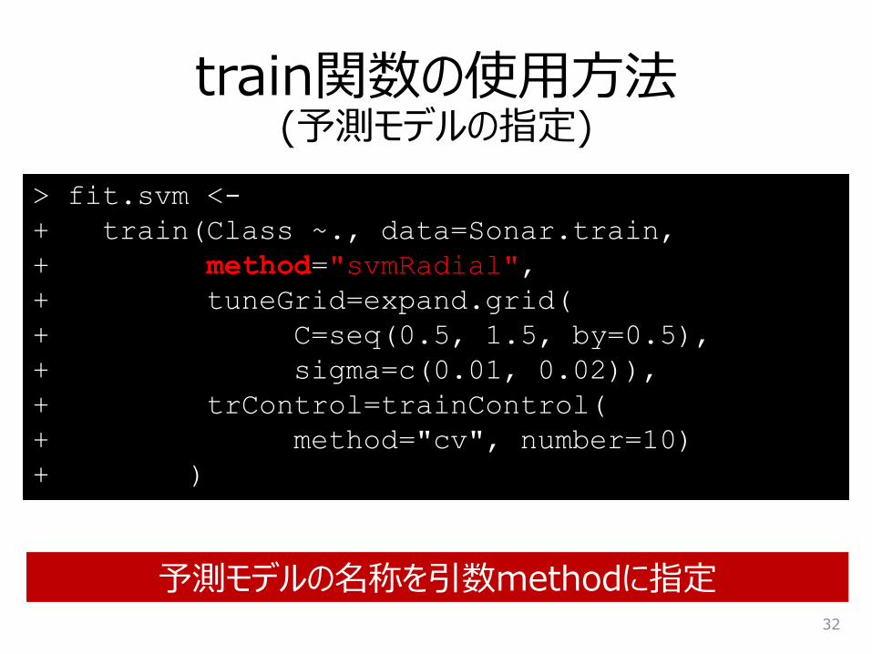
train関数の使用方法(予測モデルの指定)
32
> fit.svm <-
+ train(Class ~., data=Sonar.train,
+ method="svmRadial",
+ tuneGrid=expand.grid(
+ C=seq(0.5, 1.5, by=0.5),
+ sigma=c(0.01, 0.02)),
+ trControl=trainControl(
+ method="cv", number=10)
+ )
予測モデルの名称を引数methodに指定
train関数の使用方法(予測モデルの指定)
33
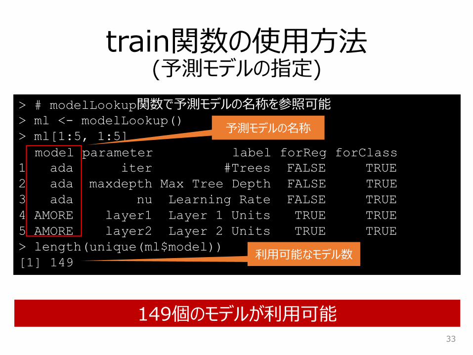
> # modelLookup関数で予測モデルの名称を参照可能> ml <- modelLookup()
> ml[1:5, 1:5]
model parameter label forReg forClass
1 ada iter #Trees FALSE TRUE
2 ada maxdepth Max Tree Depth FALSE TRUE
3 ada nu Learning Rate FALSE TRUE
4 AMORE layer1 Layer 1 Units TRUE TRUE
5 AMORE layer2 Layer 2 Units TRUE TRUE
> length(unique(ml$model))
[1] 149
149個のモデルが利用可能
予測モデルの名称
利用可能なモデル数
train関数の使用方法(ハイパーパラメータの探索範囲の指定)
34
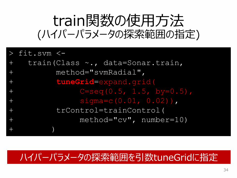
> fit.svm <-
+ train(Class ~., data=Sonar.train,
+ method="svmRadial",
+ tuneGrid=expand.grid(
+ C=seq(0.5, 1.5, by=0.5),
+ sigma=c(0.01, 0.02)),
+ trControl=trainControl(
+ method="cv", number=10)
+ )
ハイパーパラメータの探索範囲を引数tuneGridに指定
train関数の使用方法(リサンプリング方法の指定)
35
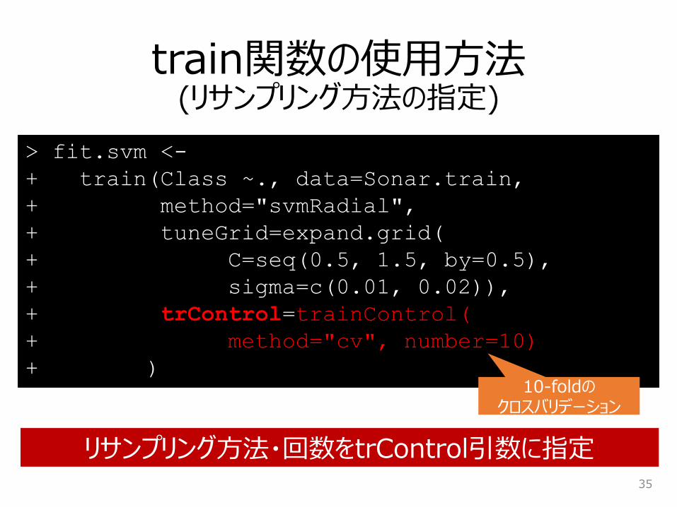
> fit.svm <-
+ train(Class ~., data=Sonar.train,
+ method="svmRadial",
+ tuneGrid=expand.grid(
+ C=seq(0.5, 1.5, by=0.5),
+ sigma=c(0.01, 0.02)),
+ trControl=trainControl(
+ method="cv", number=10)
+ )
リサンプリング方法・回数をtrControl引数に指定
10-foldのクロスバリデーション
train関数の実行結果
36
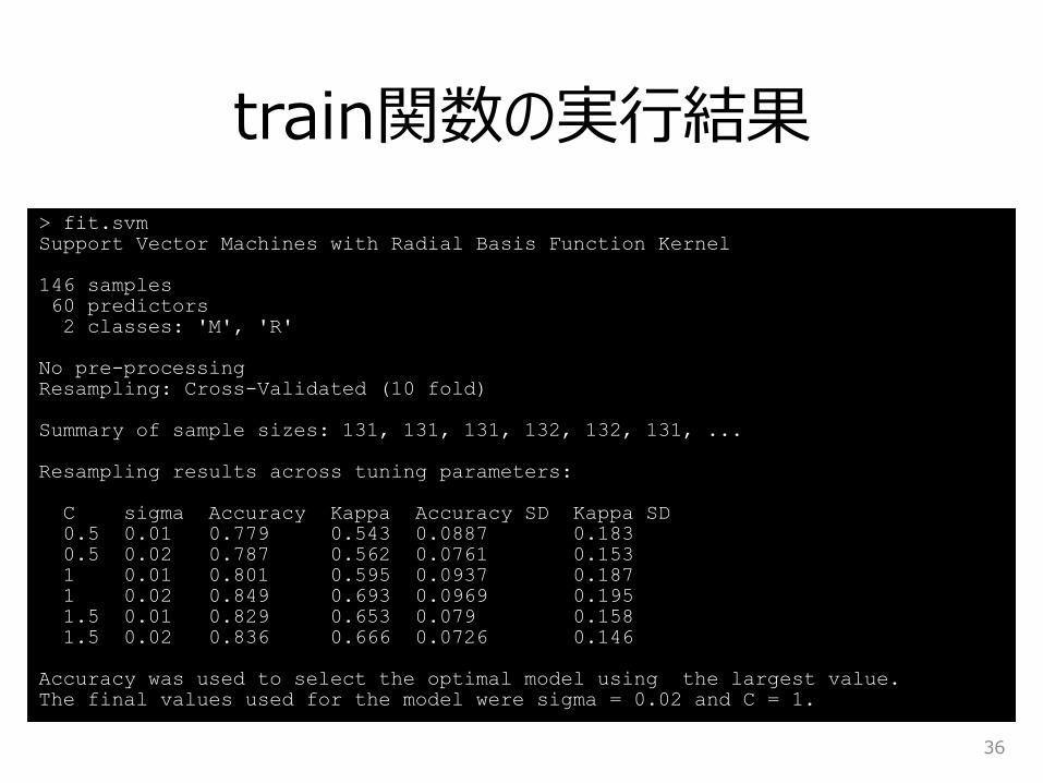
> fit.svm
Support Vector Machines with Radial Basis Function Kernel
146 samples
60 predictors
2 classes: 'M', 'R'
No pre-processing
Resampling: Cross-Validated (10 fold)
Summary of sample sizes: 131, 131, 131, 132, 132, 131, ...
Resampling results across tuning parameters:
C sigma Accuracy Kappa Accuracy SD Kappa SD
0.5 0.01 0.779 0.543 0.0887 0.183
0.5 0.02 0.787 0.562 0.0761 0.153
1 0.01 0.801 0.595 0.0937 0.187
1 0.02 0.849 0.693 0.0969 0.195
1.5 0.01 0.829 0.653 0.079 0.158
1.5 0.02 0.836 0.666 0.0726 0.146
Accuracy was used to select the optimal model using the largest value.
The final values used for the model were sigma = 0.02 and C = 1.
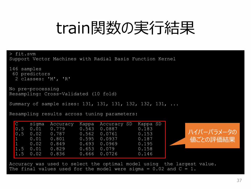
train関数の実行結果
37
> fit.svm
Support Vector Machines with Radial Basis Function Kernel
146 samples
60 predictors
2 classes: 'M', 'R'
No pre-processing
Resampling: Cross-Validated (10 fold)
Summary of sample sizes: 131, 131, 131, 132, 132, 131, ...
Resampling results across tuning parameters:
C sigma Accuracy Kappa Accuracy SD Kappa SD
0.5 0.01 0.779 0.543 0.0887 0.183
0.5 0.02 0.787 0.562 0.0761 0.153
1 0.01 0.801 0.595 0.0937 0.187
1 0.02 0.849 0.693 0.0969 0.195
1.5 0.01 0.829 0.653 0.079 0.158
1.5 0.02 0.836 0.666 0.0726 0.146
Accuracy was used to select the optimal model using the largest value.
The final values used for the model were sigma = 0.02 and C = 1.
ハイパーパラメータの値ごとの評価結果

train関数の実行結果
38
> fit.svm
Support Vector Machines with Radial Basis Function Kernel
146 samples
60 predictors
2 classes: 'M', 'R'
No pre-processing
Resampling: Cross-Validated (10 fold)
Summary of sample sizes: 131, 131, 131, 132, 132, 131, ...
Resampling results across tuning parameters:
C sigma Accuracy Kappa Accuracy SD Kappa SD
0.5 0.01 0.779 0.543 0.0887 0.183
0.5 0.02 0.787 0.562 0.0761 0.153
1 0.01 0.801 0.595 0.0937 0.187
1 0.02 0.849 0.693 0.0969 0.195 1.5 0.01 0.829 0.653 0.079 0.158
1.5 0.02 0.836 0.666 0.0726 0.146
Accuracy was used to select the optimal model using the largest value.
The final values used for the model were sigma = 0.02 and C = 1.
Accuracyが最大のモデルを
最適モデルと判断
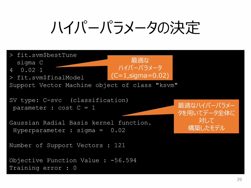
ハイパーパラメータの決定
39
> fit.svm$bestTune
sigma C
4 0.02 1
> fit.svm$finalModel
Support Vector Machine object of class "ksvm"
SV type: C-svc (classification)
parameter : cost C = 1
Gaussian Radial Basis kernel function.
Hyperparameter : sigma = 0.02
Number of Support Vectors : 121
Objective Function Value : -56.594
Training error : 0
最適なハイパーパラメータ
(C=1,sigma=0.02)
最適なハイパーパラメータを用いてデータ全体に
対して構築したモデル

4. 予測モデルの構築・評価 発展編
40

発展編のトピック
評価指標の変更
属性選択
不均衡データへの対応
41
評価指標の変更(デフォルトの評価指標設定の構造理解)
42
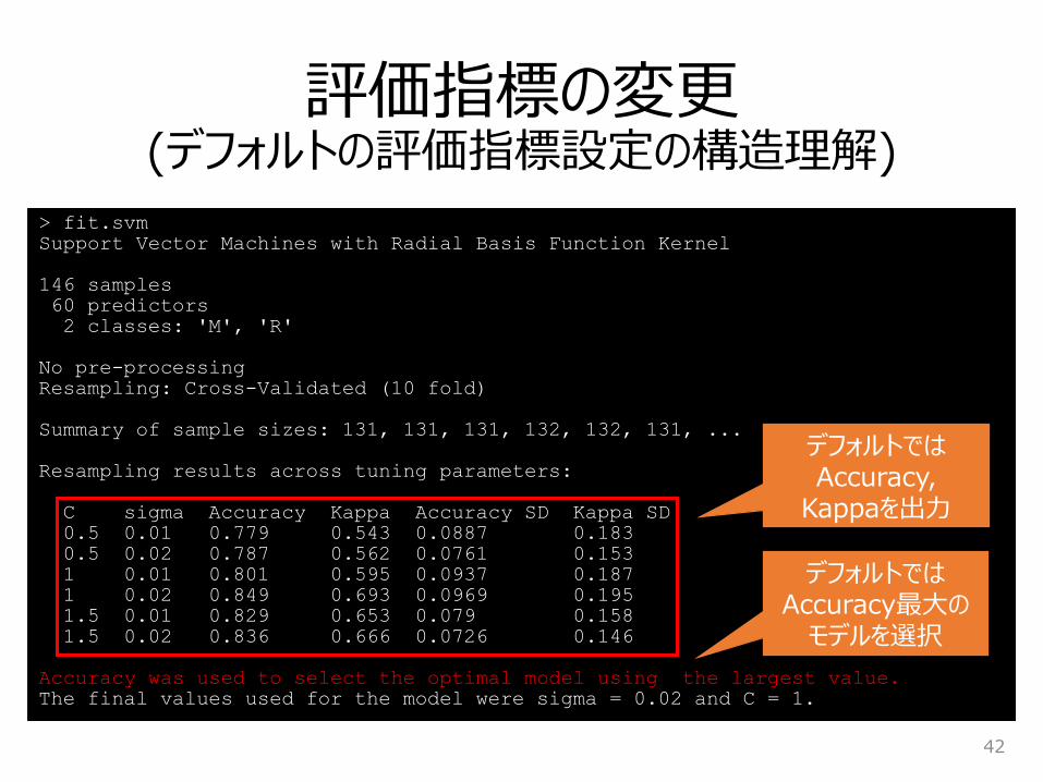
> fit.svm
Support Vector Machines with Radial Basis Function Kernel
146 samples
60 predictors
2 classes: 'M', 'R'
No pre-processing
Resampling: Cross-Validated (10 fold)
Summary of sample sizes: 131, 131, 131, 132, 132, 131, ...
Resampling results across tuning parameters:
C sigma Accuracy Kappa Accuracy SD Kappa SD
0.5 0.01 0.779 0.543 0.0887 0.183
0.5 0.02 0.787 0.562 0.0761 0.153
1 0.01 0.801 0.595 0.0937 0.187
1 0.02 0.849 0.693 0.0969 0.195
1.5 0.01 0.829 0.653 0.079 0.158
1.5 0.02 0.836 0.666 0.0726 0.146
Accuracy was used to select the optimal model using the largest value.
The final values used for the model were sigma = 0.02 and C = 1.
デフォルトではAccuracy,
Kappaを出力
デフォルトではAccuracy最大の
モデルを選択
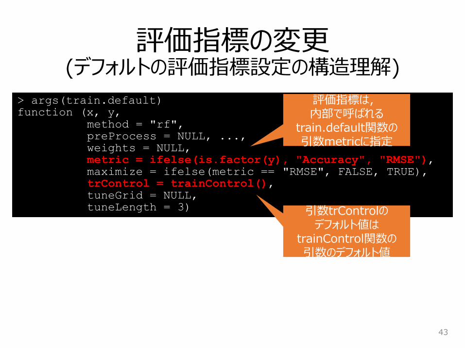
評価指標の変更(デフォルトの評価指標設定の構造理解)
43
> args(train.default)
function (x, y,
method = "rf",
preProcess = NULL, ...,
weights = NULL,
metric = ifelse(is.factor(y), "Accuracy", "RMSE"), maximize = ifelse(metric == "RMSE", FALSE, TRUE),
trControl = trainControl(), tuneGrid = NULL,
tuneLength = 3)
評価指標は,内部で呼ばれる
train.default関数の引数metricに指定
引数trControlのデフォルト値は
trainControl関数の引数のデフォルト値
> args(trainControl)
function (method = "boot",
number = ifelse(method %in% c(“cv”, "repeatedcv"),
10, 25),
repeats = ifelse(method %in% c("cv", "repeatedcv"),
1, number),
p = 0.75, initialWindow = NULL,
horizon = 1, fixedWindow = TRUE, verboseIter = FALSE,
returnData = TRUE,
returnResamp = "final", savePredictions = FALSE,
classProbs = FALSE,
summaryFunction = defaultSummary,selectionFunction = "best",
preProcOptions = list(thresh = 0.95, ICAcomp = 3, k = 5),
index = NULL, indexOut = NULL, timingSamps = 0,
predictionBounds = rep(FALSE, 2), seeds = NA,
allowParallel = TRUE)
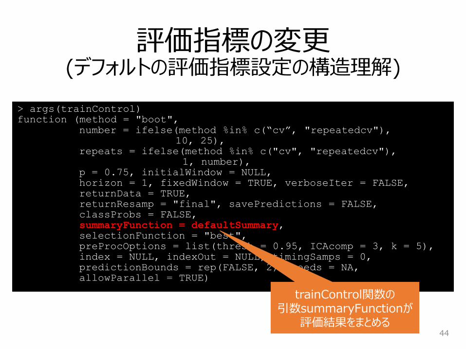
評価指標の変更(デフォルトの評価指標設定の構造理解)
44
trainControl関数の引数summaryFunctionが
評価結果をまとめる
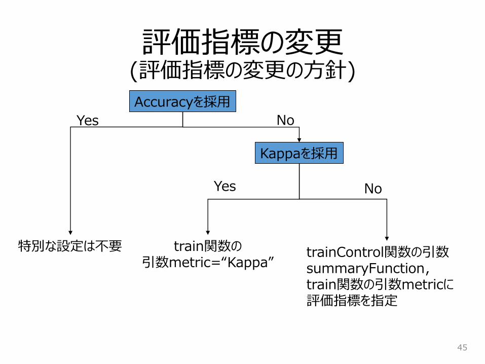
評価指標の変更(評価指標の変更の方針)
45
Accuracyを採用
trainControl関数の引数summaryFunction,train関数の引数metricに評価指標を指定
Kappaを採用
特別な設定は不要
Yes
train関数の引数metric=“Kappa”
No
Yes No
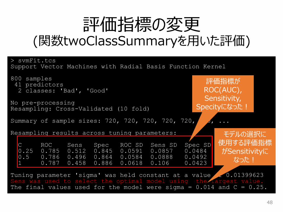
評価指標の変更(関数twoClassSummaryを用いた評価)
caretパッケージが提供するもう一つの要約関数twoClassSummaryを使用する.
twoClassSummaryは,予測モデルが出力するクラスの確率に基づいて,AUC, Sensitivity, Specificityを計算する.
46
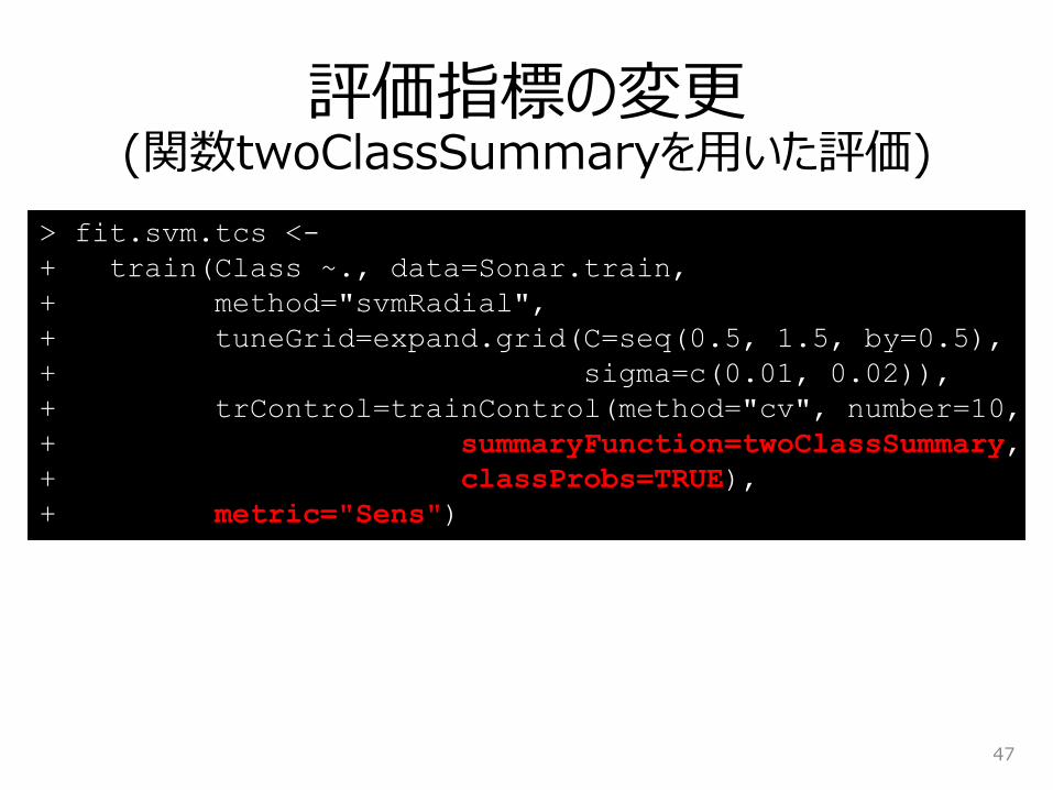
評価指標の変更(関数twoClassSummaryを用いた評価)
47
> fit.svm.tcs <-
+ train(Class ~., data=Sonar.train,
+ method="svmRadial",
+ tuneGrid=expand.grid(C=seq(0.5, 1.5, by=0.5),
+ sigma=c(0.01, 0.02)),
+ trControl=trainControl(method="cv", number=10,
+ summaryFunction=twoClassSummary,
+ classProbs=TRUE),
+ metric="Sens")
評価指標の変更(関数twoClassSummaryを用いた評価)
48
> svmFit.tcsSupport Vector Machines with Radial Basis Function Kernel
800 samples41 predictors2 classes: 'Bad', 'Good'
No pre-processingResampling: Cross-Validated (10 fold)
Summary of sample sizes: 720, 720, 720, 720, 720, 720, ...
Resampling results across tuning parameters:
C ROC Sens Spec ROC SD Sens SD Spec SD0.25 0.785 0.512 0.845 0.0591 0.0857 0.0484 0.5 0.786 0.496 0.864 0.0584 0.0888 0.0492 1 0.787 0.458 0.886 0.0618 0.106 0.0423
Tuning parameter 'sigma' was held constant at a value of 0.01399623Sens was used to select the optimal model using the largest value.The final values used for the model were sigma = 0.014 and C = 0.25.
評価指標がROC(AUC), Sensitivity,
Specityになった!
モデルの選択に使用する評価指標がSensitivityに
なった!
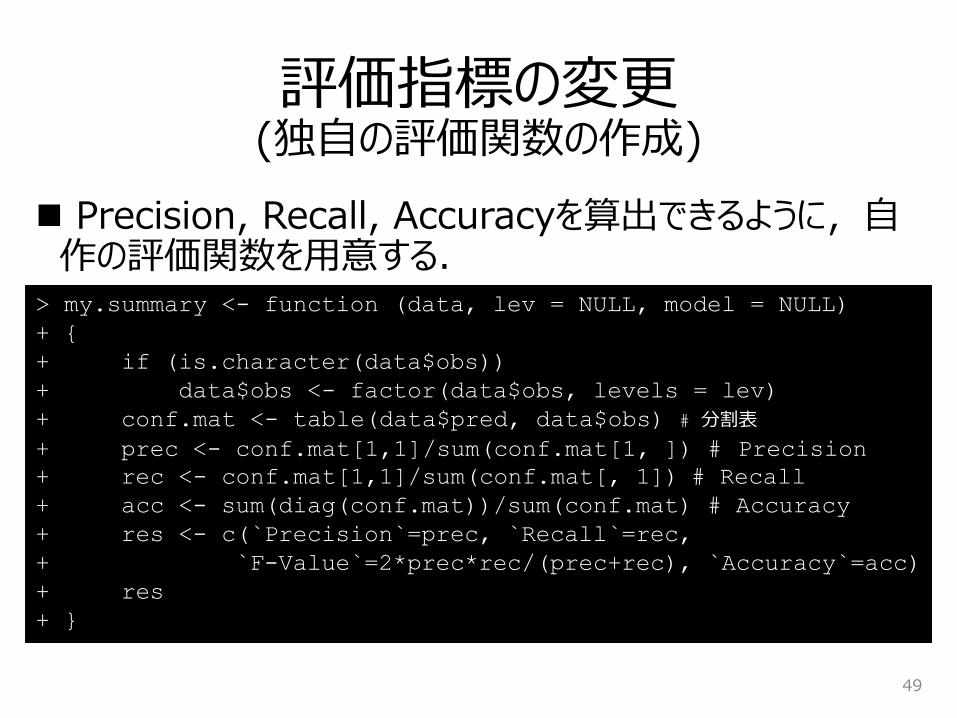
評価指標の変更(独自の評価関数の作成)
Precision, Recall, Accuracyを算出できるように,自作の評価関数を用意する.
49
> my.summary <- function (data, lev = NULL, model = NULL)
+ {
+ if (is.character(data$obs))
+ data$obs <- factor(data$obs, levels = lev)
+ conf.mat <- table(data$pred, data$obs) # 分割表
+ prec <- conf.mat[1,1]/sum(conf.mat[1, ]) # Precision
+ rec <- conf.mat[1,1]/sum(conf.mat[, 1]) # Recall
+ acc <- sum(diag(conf.mat))/sum(conf.mat) # Accuracy
+ res <- c(`Precision`=prec, `Recall`=rec,
+ `F-Value`=2*prec*rec/(prec+rec), `Accuracy`=acc)
+ res
+ }
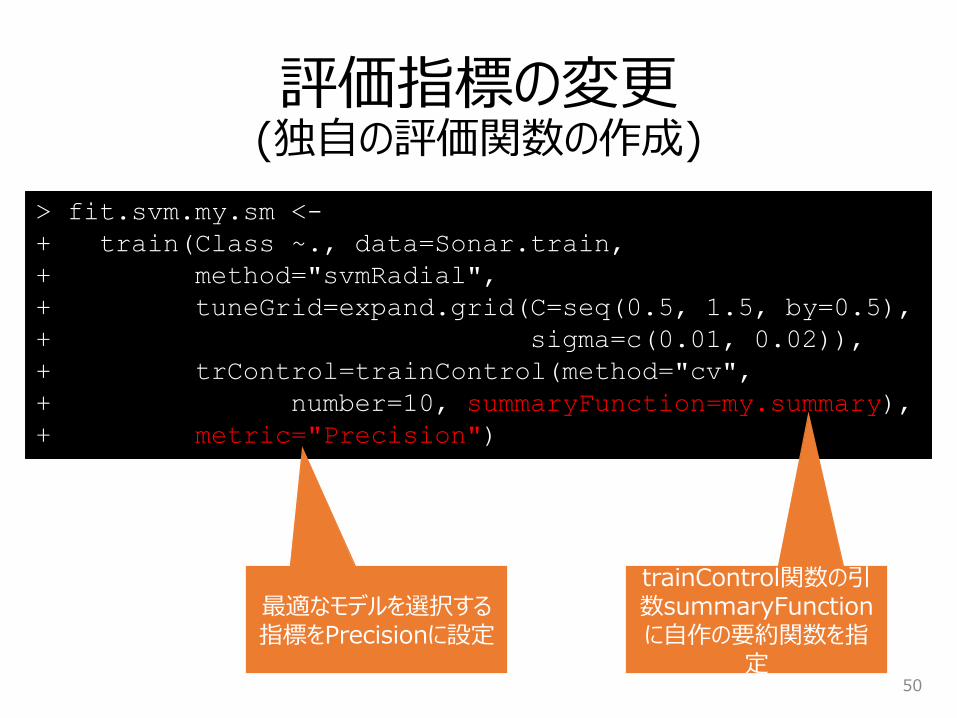
評価指標の変更(独自の評価関数の作成)
50
> fit.svm.my.sm <-
+ train(Class ~., data=Sonar.train,
+ method="svmRadial",
+ tuneGrid=expand.grid(C=seq(0.5, 1.5, by=0.5),
+ sigma=c(0.01, 0.02)),
+ trControl=trainControl(method="cv",
+ number=10, summaryFunction=my.summary),
+ metric="Precision")
trainControl関数の引数summaryFunctionに自作の要約関数を指
定
最適なモデルを選択する指標をPrecisionに設定
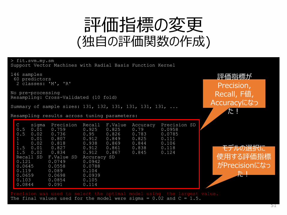
評価指標の変更(独自の評価関数の作成)
51
> fit.svm.my.smSupport Vector Machines with Radial Basis Function Kernel
146 samples60 predictors2 classes: 'M', 'R'
No pre-processingResampling: Cross-Validated (10 fold)
Summary of sample sizes: 131, 132, 131, 131, 131, 131, ...
Resampling results across tuning parameters:
C sigma Precision Recall F.Value Accuracy Precision SD0.5 0.01 0.759 0.925 0.825 0.79 0.0958 0.5 0.02 0.736 0.95 0.826 0.783 0.0785 1 0.01 0.807 0.912 0.849 0.825 0.111 1 0.02 0.818 0.938 0.869 0.844 0.106 1.5 0.01 0.827 0.912 0.861 0.838 0.118 1.5 0.02 0.834 0.912 0.867 0.845 0.124 Recall SD F.Value SD Accuracy SD0.121 0.0749 0.0942 0.0645 0.0558 0.0788 0.119 0.089 0.104 0.0659 0.0698 0.0939 0.103 0.0854 0.105 0.0844 0.091 0.114
Precision was used to select the optimal model using the largest value.The final values used for the model were sigma = 0.02 and C = 1.5.
評価指標がPrecision,
Recall, F値, Accuracyになっ
た!
モデルの選択に使用する評価指標がPrecisionになっ
た!
属性選択(feature selection)
予測モデルが過学習(overfitting)しないように,属性を選択する.
属性選択については,前回のTokyo.Rの@srctadaさんの発表が詳しい.
52
属性選択(feature selection)
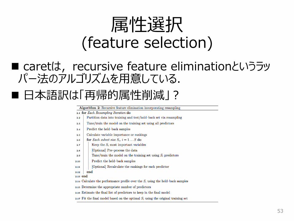
caretは,recursive feature eliminationというラッパー法のアルゴリズムを用意している.
日本語訳は「再帰的属性削減」?
53
属性選択(feature selection)
54
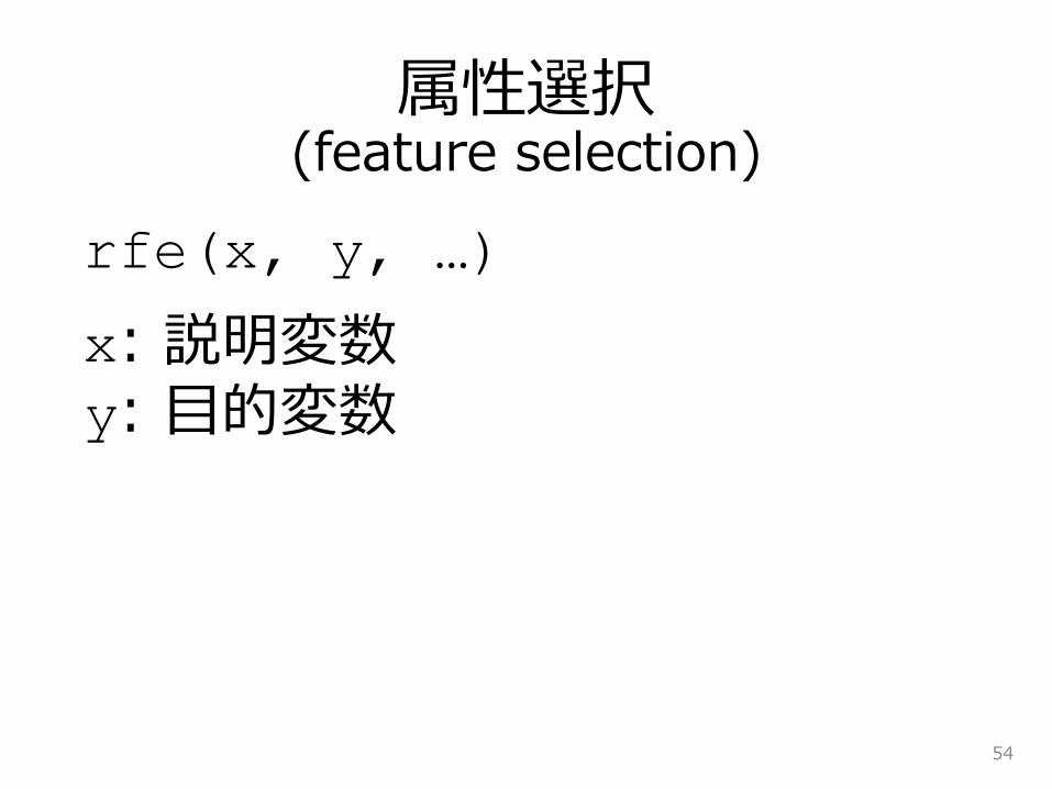
rfe(x, y, …)
x: 説明変数y: 目的変数
属性選択(feature selection)
55
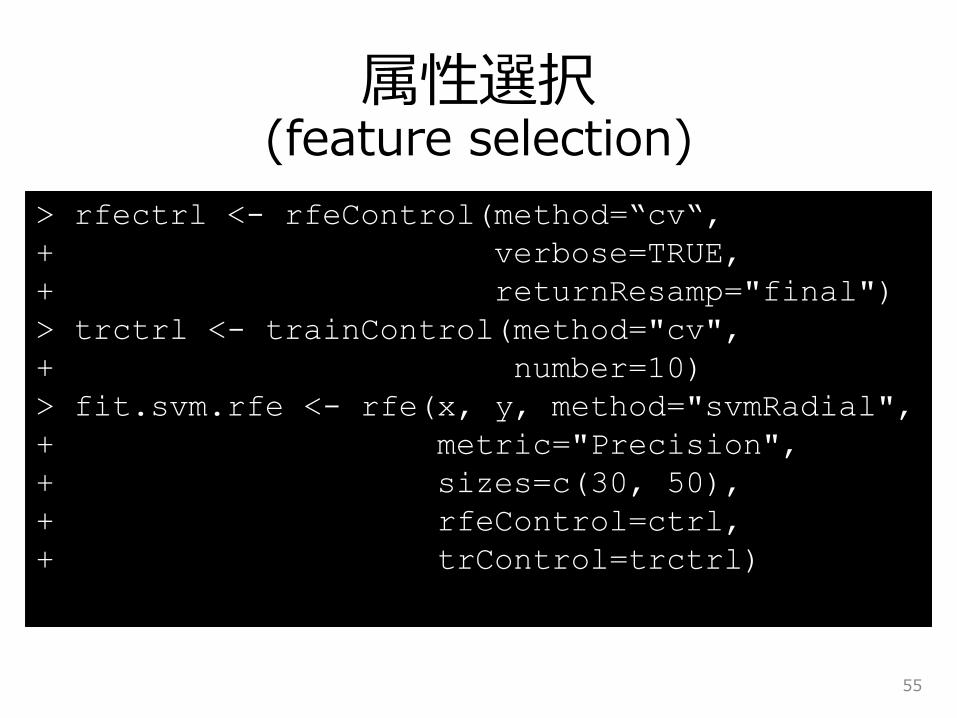
> rfectrl <- rfeControl(method=“cv“,
+ verbose=TRUE,
+ returnResamp="final")
> trctrl <- trainControl(method="cv",
+ number=10)
> fit.svm.rfe <- rfe(x, y, method="svmRadial",
+ metric="Precision",
+ sizes=c(30, 50),
+ rfeControl=ctrl,
+ trControl=trctrl)
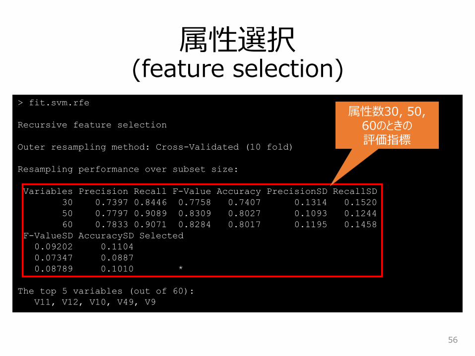
属性選択(feature selection)
56
> fit.svm.rfe
Recursive feature selection
Outer resampling method: Cross-Validated (10 fold)
Resampling performance over subset size:
Variables Precision Recall F-Value Accuracy PrecisionSD RecallSD
30 0.7397 0.8446 0.7758 0.7407 0.1314 0.1520
50 0.7797 0.9089 0.8309 0.8027 0.1093 0.1244
60 0.7833 0.9071 0.8284 0.8017 0.1195 0.1458
F-ValueSD AccuracySD Selected
0.09202 0.1104
0.07347 0.0887
0.08789 0.1010 *
The top 5 variables (out of 60):
V11, V12, V10, V49, V9
属性数30, 50, 60のときの評価指標
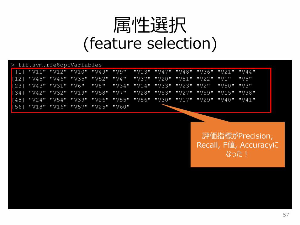
属性選択(feature selection)
57
> fit.svm.rfe$optVariables
[1] "V11" "V12" "V10" "V49" "V9" "V13" "V47" "V48" "V36" "V21" "V44"
[12] "V45" "V46" "V35" "V52" "V4" "V37" "V20" "V51" "V22" "V1" "V5"
[23] "V43" "V31" "V6" "V8" "V34" "V14" "V33" "V23" "V2" "V50" "V3"
[34] "V42" "V32" "V19" "V58" "V7" "V28" "V53" "V27" "V59" "V15" "V38"
[45] "V24" "V54" "V39" "V26" "V55" "V56" "V30" "V17" "V29" "V40" "V41"
[56] "V18" "V16" "V57" "V25" "V60"
評価指標がPrecision, Recall, F値, Accuracyに
なった!

不均衡データへの対応
クラス分類問題で扱うデータは,往々にしてクラスのサンプル数に偏りがある.
このような不均衡データに対して予測モデルを構築すると,負例の特徴を学習し,負例と予測するモデルになりやすい.
不均衡データへの代表的な対応方法は, コスト考慮型学習
サンプリング(正例のアップサンプリング/負例のダウンサンプリング/ハイブリッド)
58

不均衡データへの対応
SVMのコスト考慮型学習,ハイブリッドのサンプリングの代表的な手法であるSMOTEについては,以下のスライドを参照.
59
@sfchaos, 不均衡データのクラス分類, 第20回Tokyo.R

4. まとめ
60

機械学習を用いて予測モデル構築・評価するにはcaretパッケージが便利!!
61
参考文献
Max Kuhn and Kjell Johnson,
Applied predictive modeling, Springer, 2012.
62

参考文献
@dichika, caretパッケージ紹介
63
http://www.slideshare.net/dichika/tokyo-r11caret