9550395503 統資軟體課程講義統資軟體課程講義

Data Structures in Maple

指導教授：蔡桂宏 博士學生 ：林師賢學號 : 95356035

• Basic data structures in Maple

• Data vs. data structure vs. data type

• Nested data structures

• Expressions as data structures

• Expression trees

• Why are expression trees important?

• Some other basic data types

• Tables and arrays

• Structured data types

Basic data structures in Maple

• Expression sequences • Lists • Sets • Some numeric data types • Names (or symbols) • Strings • Equations and inequalities • Ranges• Function calls

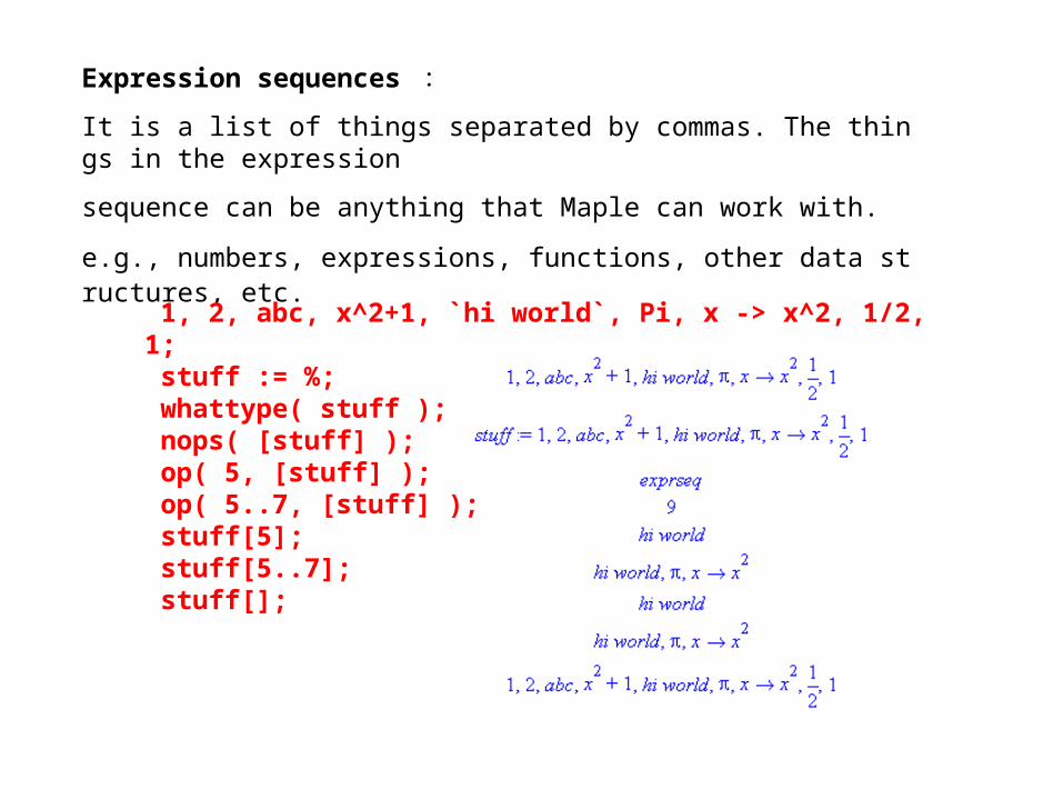
Expression sequences ：

It is a list of things separated by commas. The things in the expression

sequence can be anything that Maple can work with.

e.g., numbers, expressions, functions, other data structures, etc.

1, 2, abc, x^2+1, `hi world`, Pi, x -> x^2, 1/2, 1; stuff := %; whattype( stuff ); nops( [stuff] ); op( 5, [stuff] ); op( 5..7, [stuff] ); stuff[5]; stuff[5..7]; stuff[];

seq1 := a, b, c, d;seq2 := b, a, c, d;evalb( seq1=seq2 );seq1 := a, b, c, d;seq2 := u, v, w, x, y, z;seq3 := seq1, seq2;seq3 := seq2[1..3], seq1, seq2[4..6];

whattype( 'NULL' ); whattype( NULL ); nops( [NULL] );

solve( cos(ln(x))=tan(x)^2, x ); #NULL whattype( solve(cos(ln(x))=tan(x)^2, x) ); evalb( solve( cos(ln(x))=tan(x)^2, x ) = NULL );

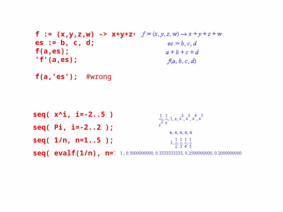
f := (x,y,z,w) -> x+y+z+w;es := b, c, d;f(a,es);'f'(a,es);

f(a,'es'); #wrong

seq( x^i, i=-2..5 );

seq( Pi, i=-2..2 );

seq( 1/n, n=1..5 );

seq( evalf(1/n), n=1..5 );

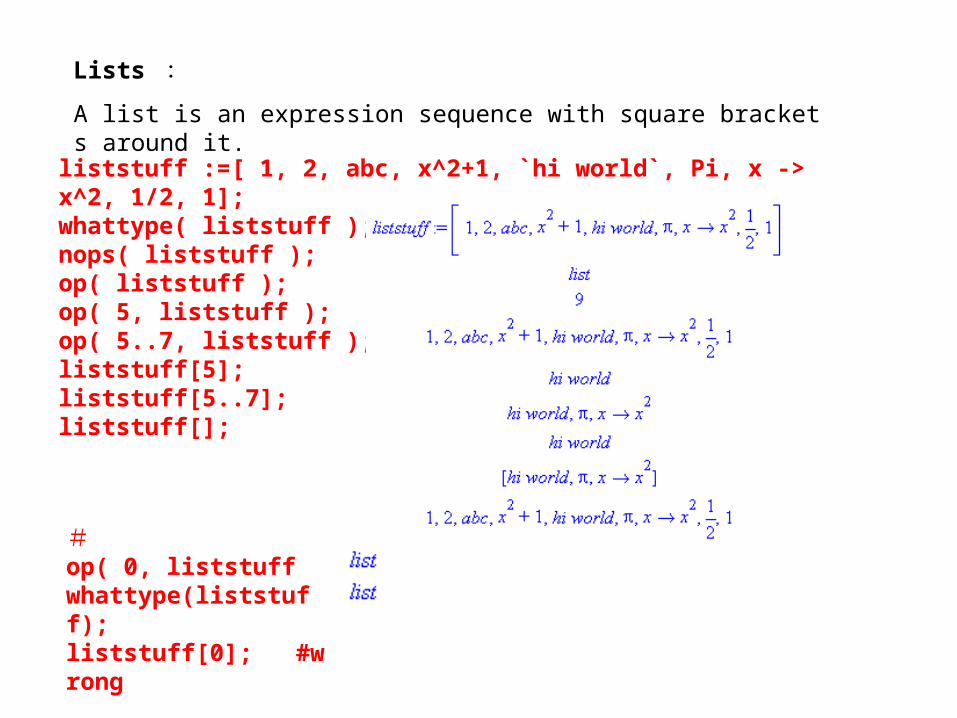
Lists ：

A list is an expression sequence with square brackets around it.

liststuff :=[ 1, 2, abc, x^2+1, `hi world`, Pi, x -> x^2, 1/2, 1];whattype( liststuff );nops( liststuff );op( liststuff );op( 5, liststuff );op( 5..7, liststuff );liststuff[5];liststuff[5..7];liststuff[];

＃op( 0, liststuff );whattype(liststuff);liststuff[0]; #wrong

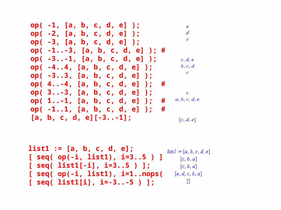
op( -1, [a, b, c, d, e] );op( -2, [a, b, c, d, e] );op( -3, [a, b, c, d, e] );op( -1..-3, [a, b, c, d, e] ); #wrongop( -3..-1, [a, b, c, d, e] );op( -4..4, [a, b, c, d, e] );op( -3..3, [a, b, c, d, e] );op( 4..-4, [a, b, c, d, e] ); #wrongop( 3..-3, [a, b, c, d, e] );op( 1..-1, [a, b, c, d, e] ); #list allop( -1..1, [a, b, c, d, e] ); #wrong[a, b, c, d, e][-3..-1];

list1 := [a, b, c, d, e];[ seq( op(-i, list1), i=3..5 ) ];[ seq( list1[-i], i=3..5 ) ];[ seq( op(-i, list1), i=1..nops(list1) ) ];[ seq( list1[i], i=-3..-5 ) ];

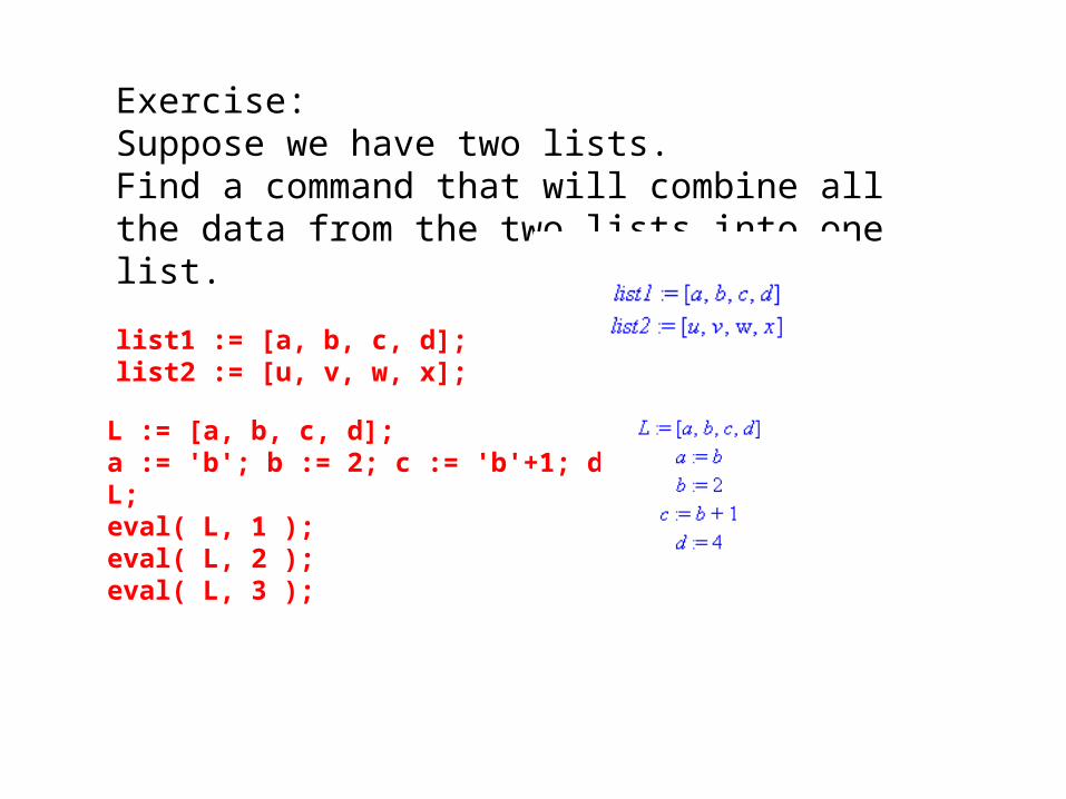
Exercise: Suppose we have two lists. Find a command that will combine all the data from the two lists into one list.

list1 := [a, b, c, d];list2 := [u, v, w, x];

L := [a, b, c, d];a := 'b'; b := 2; c := 'b'+1; d := 4;L;eval( L, 1 );eval( L, 2 );eval( L, 3 );

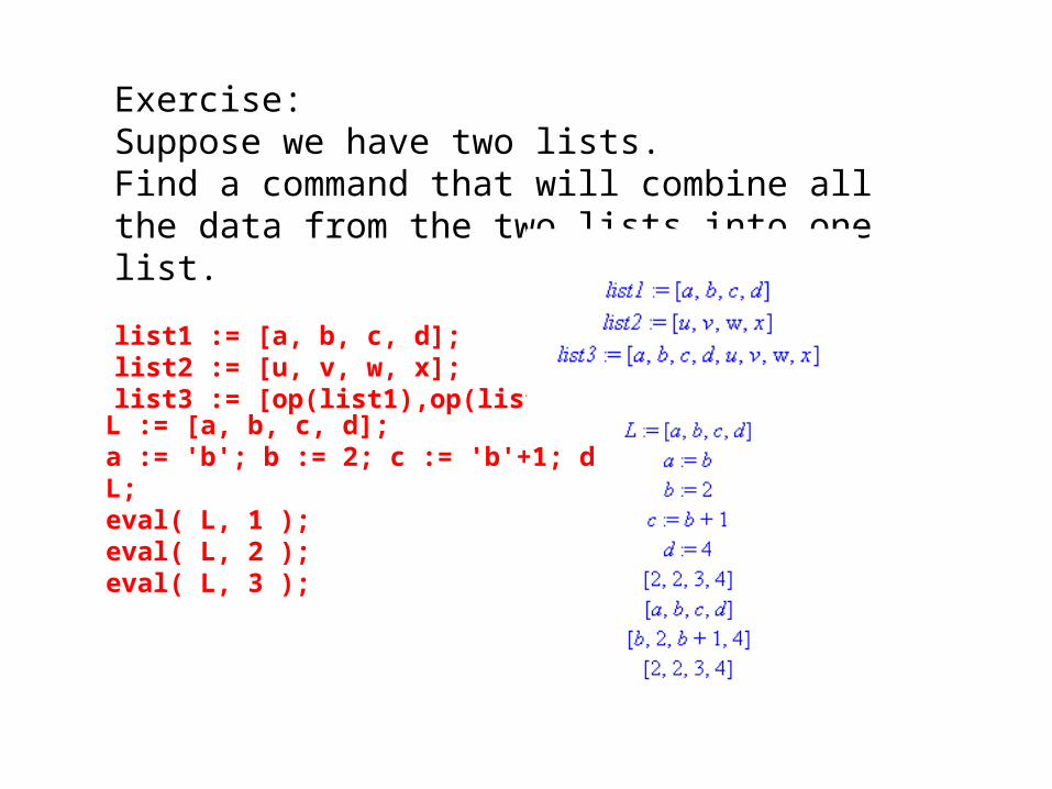
Exercise: Suppose we have two lists. Find a command that will combine all the data from the two lists into one list.

list1 := [a, b, c, d];list2 := [u, v, w, x];list3 := [op(list1),op(list2)];

L := [a, b, c, d];a := 'b'; b := 2; c := 'b'+1; d := 4;L;eval( L, 1 );eval( L, 2 );eval( L, 3 );

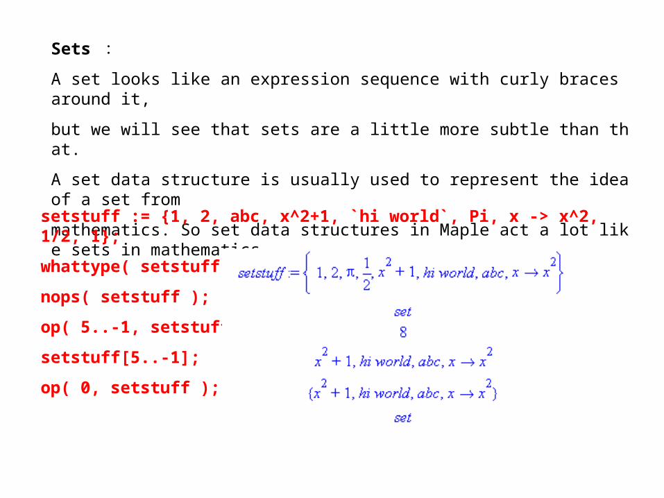
Sets ：

A set looks like an expression sequence with curly braces around it,

but we will see that sets are a little more subtle than that.

A set data structure is usually used to represent the idea of a set from

mathematics. So set data structures in Maple act a lot like sets in mathematics.

setstuff := {1, 2, abc, x^2+1, `hi world`, Pi, x -> x^2, 1/2, 1};

whattype( setstuff );

nops( setstuff );

op( 5..-1, setstuff );

setstuff[5..-1];

op( 0, setstuff );

We can convert a set into an expression sequence by using the op command.setstuff := {1, 2, abc, x^2+1, `hi world`, Pi, x -> x^2, 1/2, 1};op( setstuff );

We can convert a set into a list by using op and a pair of brackets.

[op( setstuff )];

We can convert a list into a set

listtuff:=[1, 2, abc, x^2+1, `hi world`, Pi, x -> x^2, 1/2, 1];{op(listtuff)};

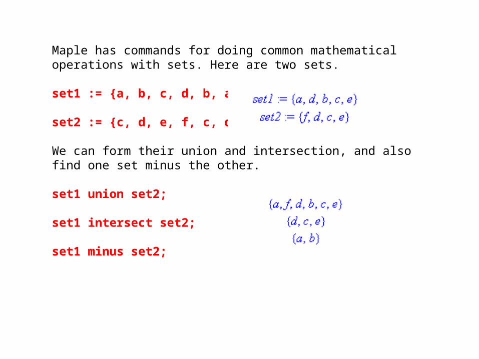
Maple has commands for doing common mathematical operations with sets. Here are two sets.

set1 := {a, b, c, d, b, a, e };

set2 := {c, d, e, f, c, d};

We can form their union and intersection, and also find one set minus the other.

set1 union set2;

set1 intersect set2;

set1 minus set2;

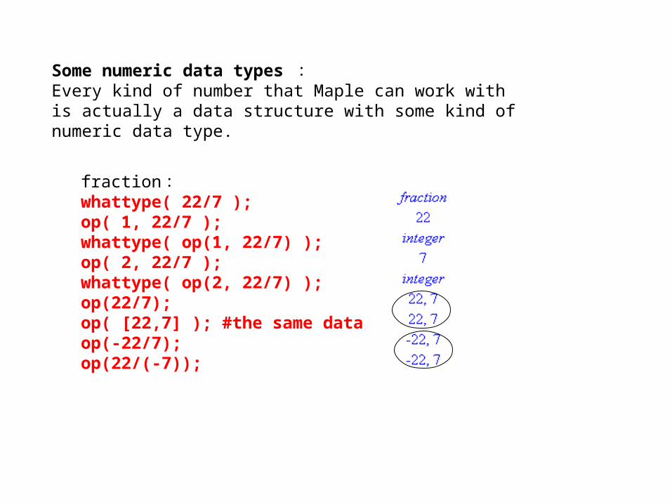
Some numeric data types ：Every kind of number that Maple can work with is actually a data structure with some kind of numeric data type.

fraction ：whattype( 22/7 );op( 1, 22/7 );whattype( op(1, 22/7) );op( 2, 22/7 );whattype( op(2, 22/7) );op(22/7);op( [22,7] ); #the same data itemsop(-22/7);op(22/(-7));

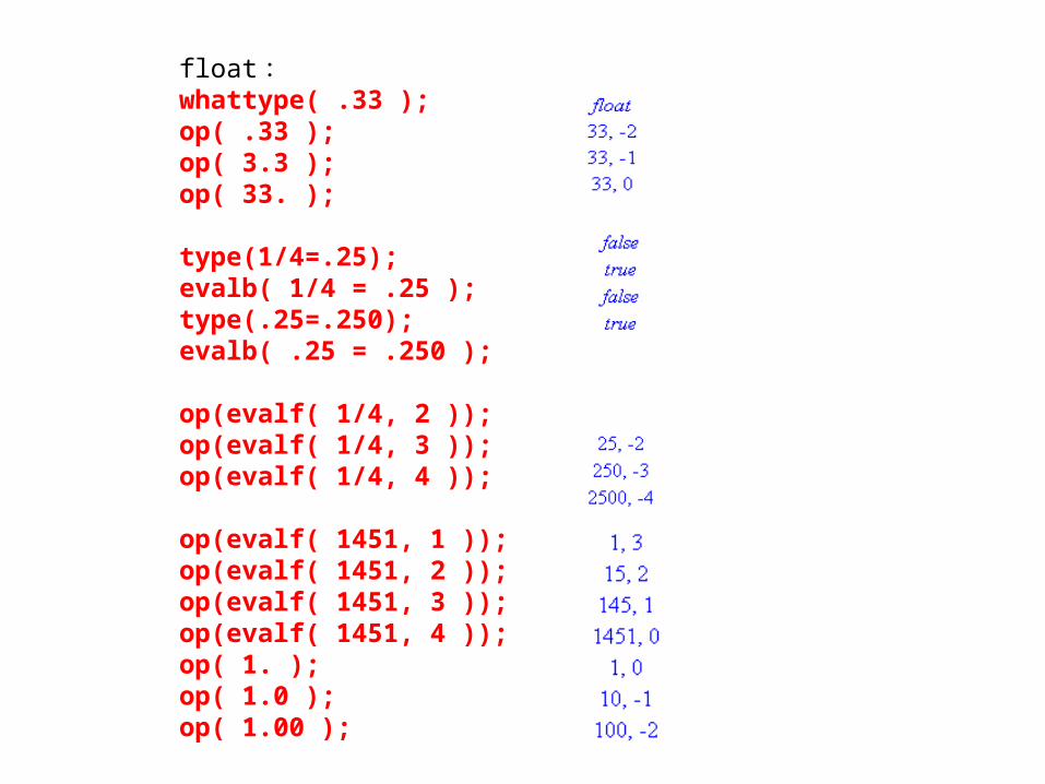
float ：whattype( .33 ); op( .33 );op( 3.3 );op( 33. );

type(1/4=.25);evalb( 1/4 = .25 );type(.25=.250);evalb( .25 = .250 );

op(evalf( 1/4, 2 ));op(evalf( 1/4, 3 ));op(evalf( 1/4, 4 ));

op(evalf( 1451, 1 ));op(evalf( 1451, 2 ));op(evalf( 1451, 3 ));op(evalf( 1451, 4 ));op( 1. );op( 1.0 );op( 1.00 );

22./7;whattype( % );op( %% );3.4e6;op( % );Float(234,5);op( % );22./7 + 2e1 - Float(-3,-2);

evalf( Pi^(Pi^(Pi^Pi)) );op( % );%[2];whattype( % );

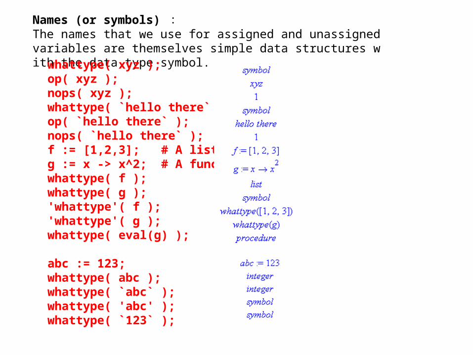
Names (or symbols) ：The names that we use for assigned and unassigned variables are themselves simple data structures with the data type symbol.

whattype( xyz ); op( xyz );nops( xyz );whattype( `hello there` );op( `hello there` );nops( `hello there` );f := [1,2,3]; # A list.g := x -> x^2; # A function.whattype( f );whattype( g );'whattype'( f );'whattype'( g );whattype( eval(g) );

abc := 123;whattype( abc );whattype( `abc` );whattype( 'abc' );whattype( `123` );

Strings ：Strings are a data structure made up of characters, just like the symbol data structure described in the last subsection. However, strings are defined in Maple using the double quote key rather than the left quote key used for symbols.

evalb( `hello world`="hello world" );whattype( `hello world` );whattype( "hello world" );nops( `hello world` );nops( "hello world" );op( `hello world` );op( "hello world" );convert( `hello world`, string );

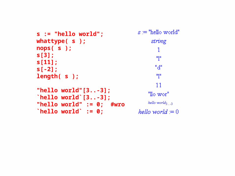
s := "hello world";whattype( s );nops( s );s[3];s[11];s[-2];length( s );

"hello world"[3..-3];`hello world`[3..-3];"hello world" := 0; #wrong`hello world` := 0;

Equations and inequalities ：It turns out that Maple considers an equation to be a data structure with data type equation. An equation data structure always has two operands, the left and right hand sides of the equation.

whattype( y = x^2 );op( y = x^2 );op( 1, y = x^2 ); op( 2, y = x^2 );lhs( y = x^2 );rhs( y = x^2 );

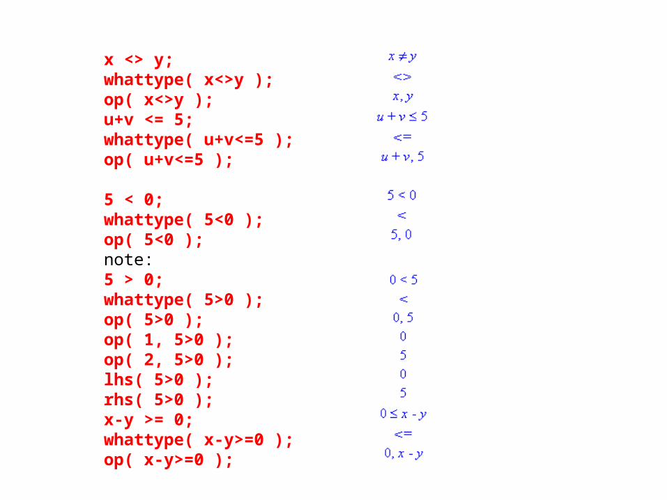
x <> y;whattype( x<>y );op( x<>y );u+v <= 5;whattype( u+v<=5 );op( u+v<=5 );

5 < 0;whattype( 5<0 );op( 5<0 );note:5 > 0;whattype( 5>0 );op( 5>0 );op( 1, 5>0 );op( 2, 5>0 );lhs( 5>0 );rhs( 5>0 );x-y >= 0;whattype( x-y>=0 );op( x-y>=0 );

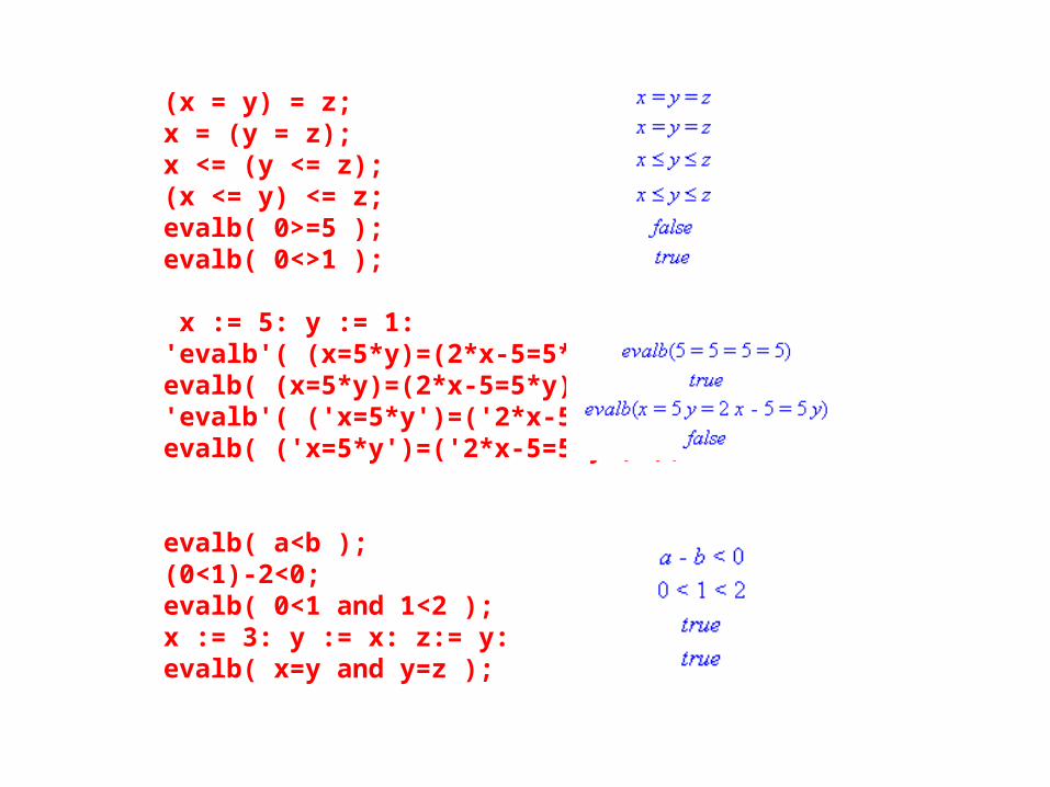
(x = y) = z;x = (y = z);x <= (y <= z);(x <= y) <= z;evalb( 0>=5 );evalb( 0<>1 );

x := 5: y := 1:'evalb'( (x=5*y)=(2*x-5=5*y) );evalb( (x=5*y)=(2*x-5=5*y) );'evalb'( ('x=5*y')=('2*x-5=5*y') );evalb( ('x=5*y')=('2*x-5=5*y') );

evalb( a<b );(0<1)-2<0;evalb( 0<1 and 1<2 );x := 3: y := x: z:= y:evalb( x=y and y=z );

Ranges ：In this subsection we show that the "dot dot" operator (..) is really used by Maple to define a data structure, with the data type range, that holds exactly two pieces of data

r := p..p^2;whattype( r );op( r );seq( i, i=r );#wrongw||(r);p := 2;w||(r);seq( i, i=r );seq( i, i=x..x^2 );#wrongseq( seq(i, i=x..x^2), x=1..3 );seq( [seq(i, i=x..x^2)], x=1..3 );

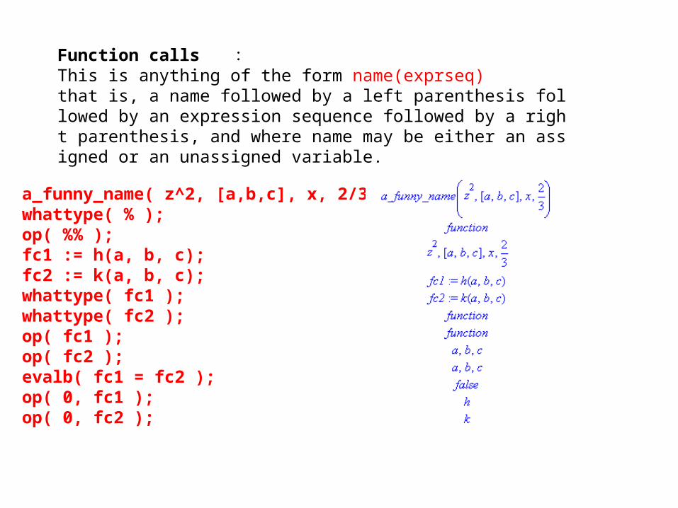
Function calls ：This is anything of the form name(exprseq)that is, a name followed by a left parenthesis followed by an expression sequence followed by a right parenthesis, and where name may be either an assigned or an unassigned variable.

a_funny_name( z^2, [a,b,c], x, 2/3 );whattype( % );op( %% );fc1 := h(a, b, c);fc2 := k(a, b, c);whattype( fc1 );whattype( fc2 );op( fc1 );op( fc2 );evalb( fc1 = fc2 );op( 0, fc1 );op( 0, fc2 );

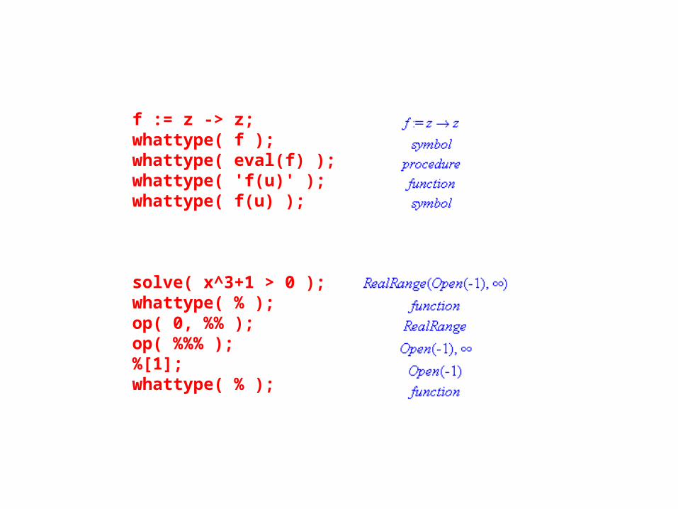
f := z -> z;whattype( f );whattype( eval(f) );whattype( 'f(u)' );whattype( f(u) );

solve( x^3+1 > 0 );whattype( % );op( 0, %% );op( %%% );%[1];whattype( % );

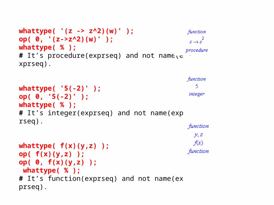
whattype( '(z -> z^2)(w)' );op( 0, '(z->z^2)(w)' );whattype( % );# It’s procedure(exprseq) and not name(exprseq).

whattype( '5(-2)' );op( 0, '5(-2)' );whattype( % );# It’s integer(exprseq) and not name(exprseq).

whattype( f(x)(y,z) );op( f(x)(y,z) );op( 0, f(x)(y,z) ); whattype( % );# It’s function(exprseq) and not name(exprseq).

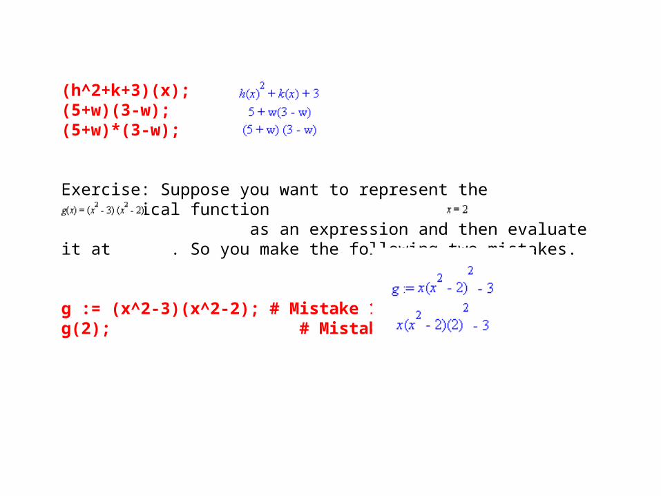
(h^2+k+3)(x);(5+w)(3-w);(5+w)*(3-w);

Exercise: Suppose you want to represent the mathematical function as an expression and then evaluate it at . So you make the following two mistakes.

g := (x^2-3)(x^2-2); # Mistake 1.g(2); # Mistake 2.

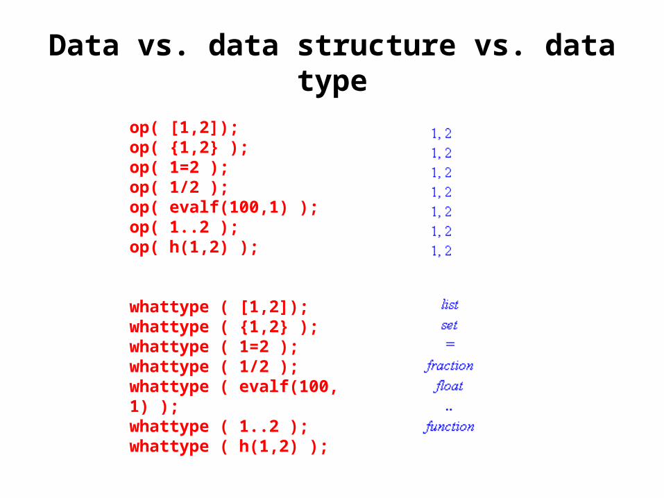
Data vs. data structure vs. data type

op( [1,2]);op( {1,2} );op( 1=2 );op( 1/2 );op( evalf(100,1) );op( 1..2 );op( h(1,2) );

whattype ( [1,2]);whattype ( {1,2} );whattype ( 1=2 );whattype ( 1/2 );whattype ( evalf(100,1) );whattype ( 1..2 );whattype ( h(1,2) );

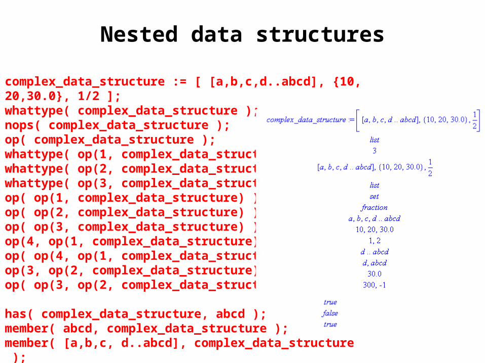
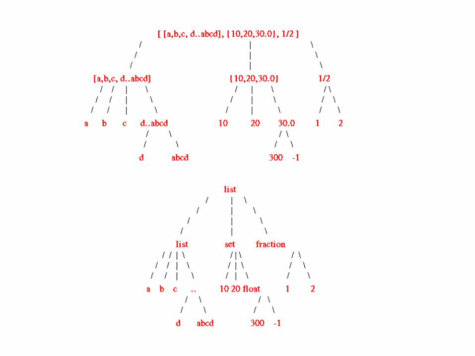
Nested data structures

complex_data_structure := [ [a,b,c,d..abcd], {10,20,30.0}, 1/2 ];whattype( complex_data_structure );nops( complex_data_structure );op( complex_data_structure );whattype( op(1, complex_data_structure) );whattype( op(2, complex_data_structure) );whattype( op(3, complex_data_structure) );op( op(1, complex_data_structure) );op( op(2, complex_data_structure) );op( op(3, complex_data_structure) );op(4, op(1, complex_data_structure) );op( op(4, op(1, complex_data_structure) ) );op(3, op(2, complex_data_structure) );op( op(3, op(2, complex_data_structure) ) );

has( complex_data_structure, abcd );member( abcd, complex_data_structure );member( [a,b,c, d..abcd], complex_data_structure );

(x=y)=(0=-2)

a:='b'; b:={'c','f'}; c:=-1; d:='a'; e:='f'; f:='g';

eval( [a, [b,c], {d,e,f}], 1 );

eval( [a, [b,c], {d,e,f}], 2 );

eval( [a, [b,c], {d,e,f}], 3 );

eval( [a, [b,c], {d,e,f}], 4 );

Expressions as data structures

quad := a*x^2+b*x+c;

whattype( quad );

nops( quad );

op( quad );

op(1, quad);

op( op(1, quad) );

whattype( op(2,op(1,quad)) );

op( op(2,op(1,quad)) );

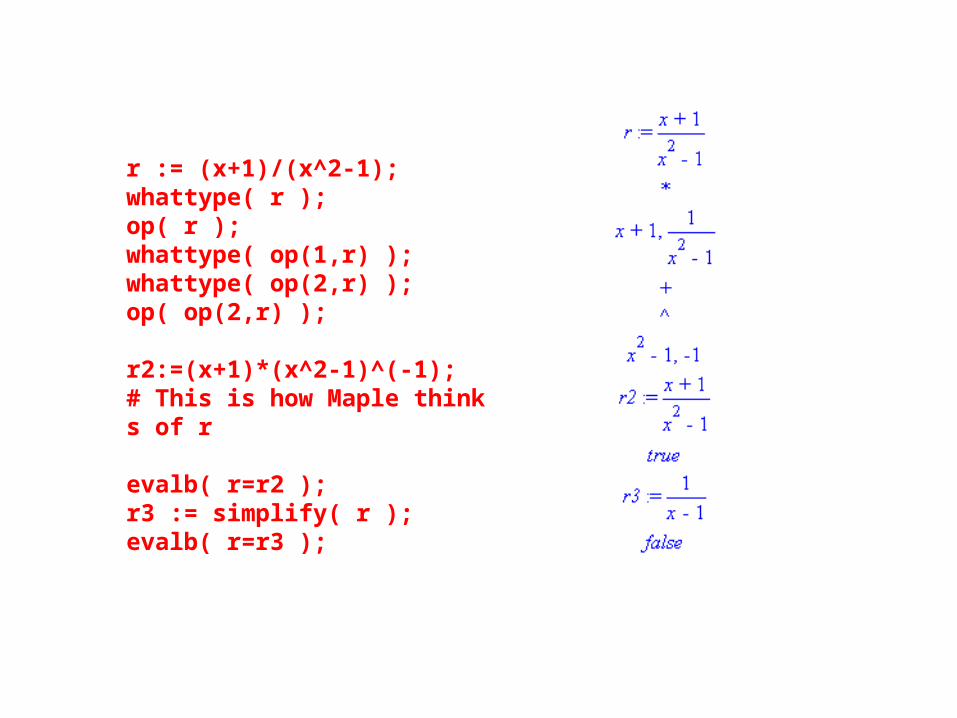
r := (x+1)/(x^2-1);whattype( r );op( r );whattype( op(1,r) ); whattype( op(2,r) );op( op(2,r) ); r2:=(x+1)*(x^2-1)^(-1); # This is how Maple thinks of r

evalb( r=r2 );r3 := simplify( r );evalb( r=r3 );

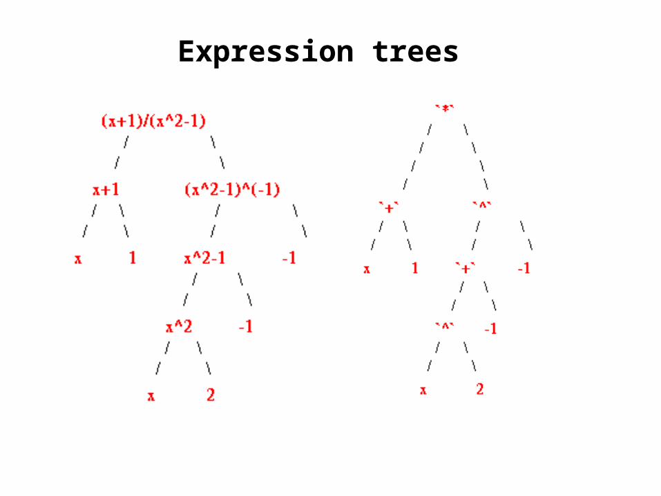
Expression trees

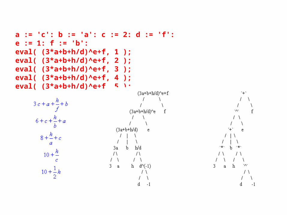
a := 'c': b := 'a': c := 2: d := 'f': e := 1: f := 'b':eval( (3*a+b+h/d)^e+f, 1 );eval( (3*a+b+h/d)^e+f, 2 );eval( (3*a+b+h/d)^e+f, 3 );eval( (3*a+b+h/d)^e+f, 4 );eval( (3*a+b+h/d)^e+f, 5 );

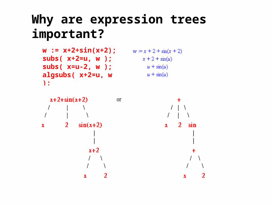
Why are expression trees important?

w := x+2+sin(x+2);subs( x+2=u, w );subs( x=u-2, w );algsubs( x+2=u, w );

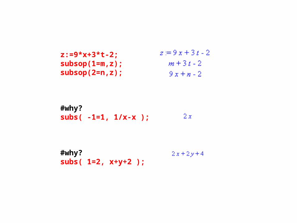
z:=9*x+3*t-2;subsop(1=m,z);subsop(2=n,z);

#why?subs( -1=1, 1/x-x );

#why?subs( 1=2, x+y+2 );

z:=9*x+3*t-2;subsop(1=m,z);subsop(2=n,z);

#why?subs( -1=1, 1/x-x );1*x^(-1)+(-1)*x;

#why?subs( 1=2, x+y+2 );1*x+1*y+2;

Some other basic data types

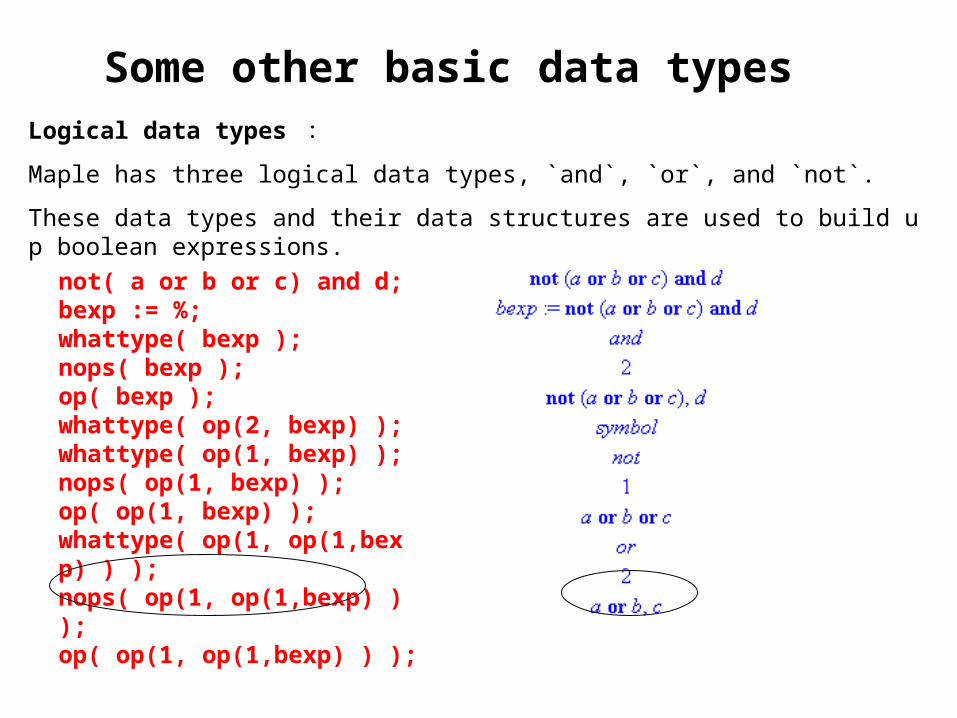
Logical data types ：

Maple has three logical data types, `and`, `or`, and `not`.

These data types and their data structures are used to build up boolean expressions.

not( a or b or c) and d;bexp := %;whattype( bexp );nops( bexp );op( bexp );whattype( op(2, bexp) );whattype( op(1, bexp) );nops( op(1, bexp) );op( op(1, bexp) );whattype( op(1, op(1,bexp) ) );nops( op(1, op(1,bexp) ) );op( op(1, op(1,bexp) ) );

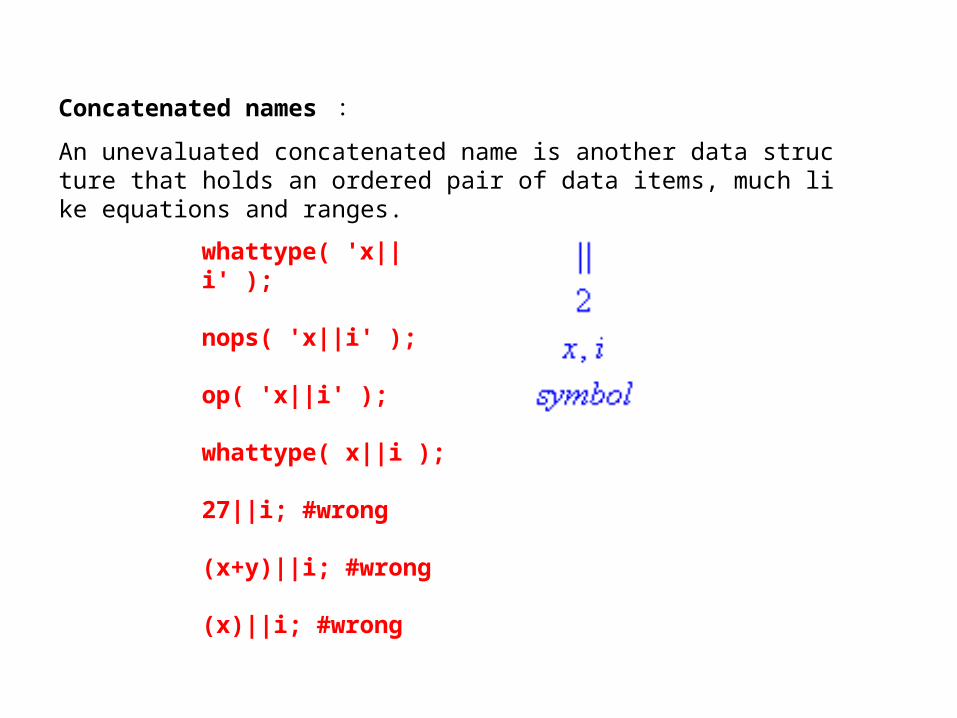
Concatenated names ：

An unevaluated concatenated name is another data structure that holds an ordered pair of data items, much like equations and ranges.

whattype( 'x||i' );

nops( 'x||i' );

op( 'x||i' );

whattype( x||i );

27||i; #wrong

(x+y)||i; #wrong

(x)||i; #wrong

whattype( 'x||i||j' );nops( 'x||i||j' );op( 'x||i||j' );op(1, 'x||i||j' );whattype( op(1, 'x||i||j' ) );op(2, 'x||i||j' );whattype( op(2, 'x||i||j' ) );

whattype( 'x||(i||j)' );nops( 'x||(i||j)' );op( 'x||(i||j)' );op(1, 'x||(i||j)' );whattype( op(1, 'x||(i||j)' ) );op(2, 'x||(i||j)' );whattype( op(2, 'x||(i||j)' ) );

(x||i)||j; #wrong

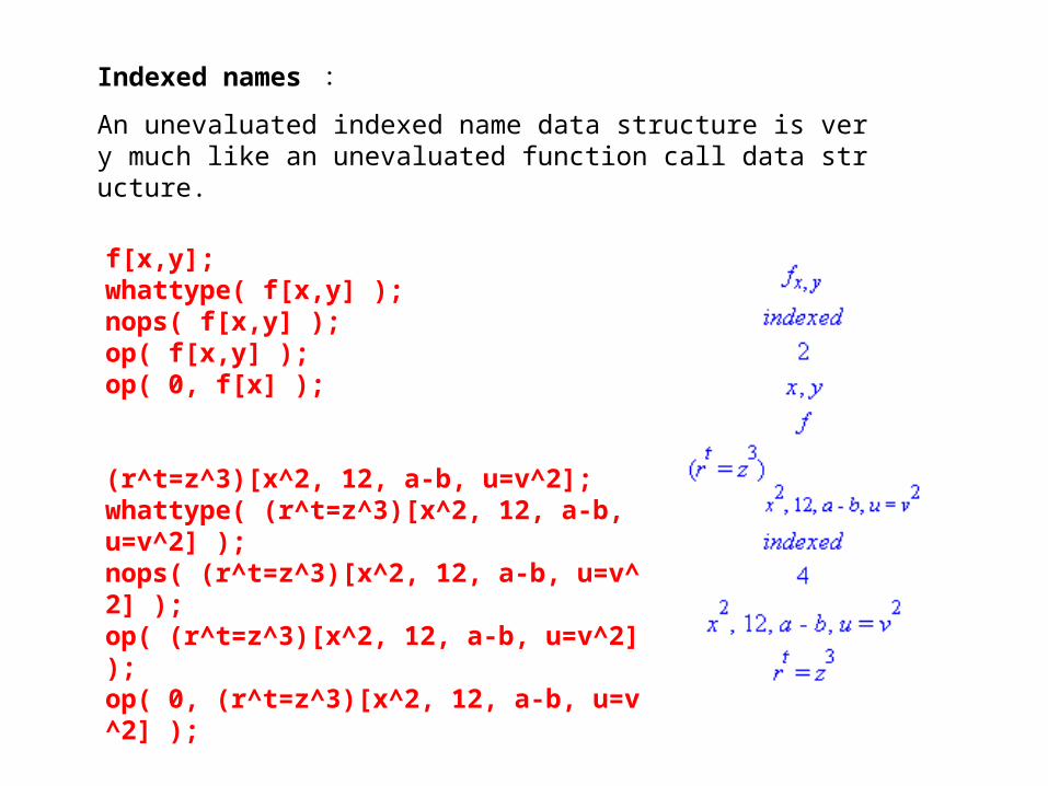
Indexed names ：

An unevaluated indexed name data structure is very much like an unevaluated function call data structure.

f[x,y];whattype( f[x,y] );nops( f[x,y] );op( f[x,y] );op( 0, f[x] );

(r^t=z^3)[x^2, 12, a-b, u=v^2];whattype( (r^t=z^3)[x^2, 12, a-b, u=v^2] );nops( (r^t=z^3)[x^2, 12, a-b, u=v^2] );op( (r^t=z^3)[x^2, 12, a-b, u=v^2] );op( 0, (r^t=z^3)[x^2, 12, a-b, u=v^2] );

[a,b,c,d][2..3];'[a,b,c,d][2..3]';whattype( '[a,b,c,d][2..3]' );op( 0, '[a,b,c,d][2..3]' );op( '[a,b,c,d][2..3]' );

op( 0, f[g[0]] );op( f[g[0]] );op( 0, f[g][0] );op( f[g][0] );op( 0, f[g][g[0]] );op( f[g][g[0]] );

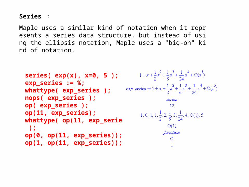
Series ：

Maple uses a similar kind of notation when it represents a series data structure, but instead of using the ellipsis notation, Maple uses a "big-oh" kind of notation.

series( exp(x), x=0, 5 );exp_series := %;whattype( exp_series );nops( exp_series );op( exp_series );op(11, exp_series);whattype( op(11, exp_series) );op(0, op(11, exp_series));op(1, op(11, exp_series));

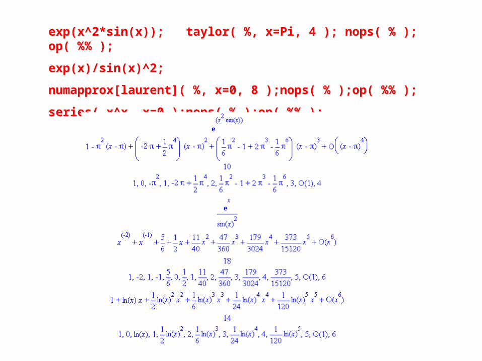
exp(x^2*sin(x)); taylor( %, x=Pi, 4 ); nops( % );op( %% );

exp(x)/sin(x)^2;

numapprox[laurent]( %, x=0, 8 );nops( % );op( %% );

series( x^x, x=0 );nops( % );op( %% );

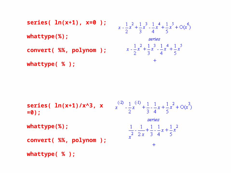
series( ln(x+1), x=0 );

whattype(%);

convert( %%, polynom );

whattype( % );

series( ln(x+1)/x^3, x=0);

whattype(%);

convert( %%, polynom );

whattype( % );

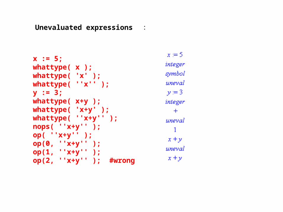
Unevaluated expressions ：

x := 5;whattype( x );whattype( 'x' );whattype( ''x'' );y := 3;whattype( x+y );whattype( 'x+y' );whattype( ''x+y'' );nops( ''x+y'' );op( ''x+y'' );op(0, ''x+y'' );op(1, ''x+y'' );op(2, ''x+y'' ); #wrong

`::` ：

The `::` data structure is, like the equation and range data structures, a data structure that holds exactly two operands that can be thought of as a left and a right hand side.

w::integer;whattype( % );op( %% );type( %%%, `::` );

proc(w::list, n::posint) op(n,w) end;op( 1, % );op( 1, %% )[1];whattype( % );op( %% );

type( 5, integer );evalb( 5::integer );type( x+y, `+` );evalb( (x+y)::`+` );

Tables and arrays Tables ：

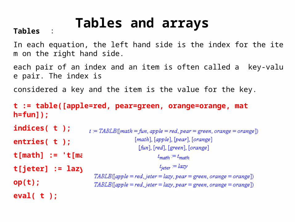
In each equation, the left hand side is the index for the item on the right hand side.

each pair of an index and an item is often called a key-value pair. The index is

considered a key and the item is the value for the key.

t := table([apple=red, pear=green, orange=orange, math=fun]);

indices( t );

entries( t );

t[math] := 't[math]';

t[jeter] := lazy;

op(t);

eval( t );

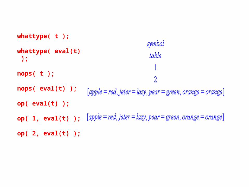
whattype( t );

whattype( eval(t) );

nops( t );

nops( eval(t) );

op( eval(t) );

op( 1, eval(t) );

op( 2, eval(t) );

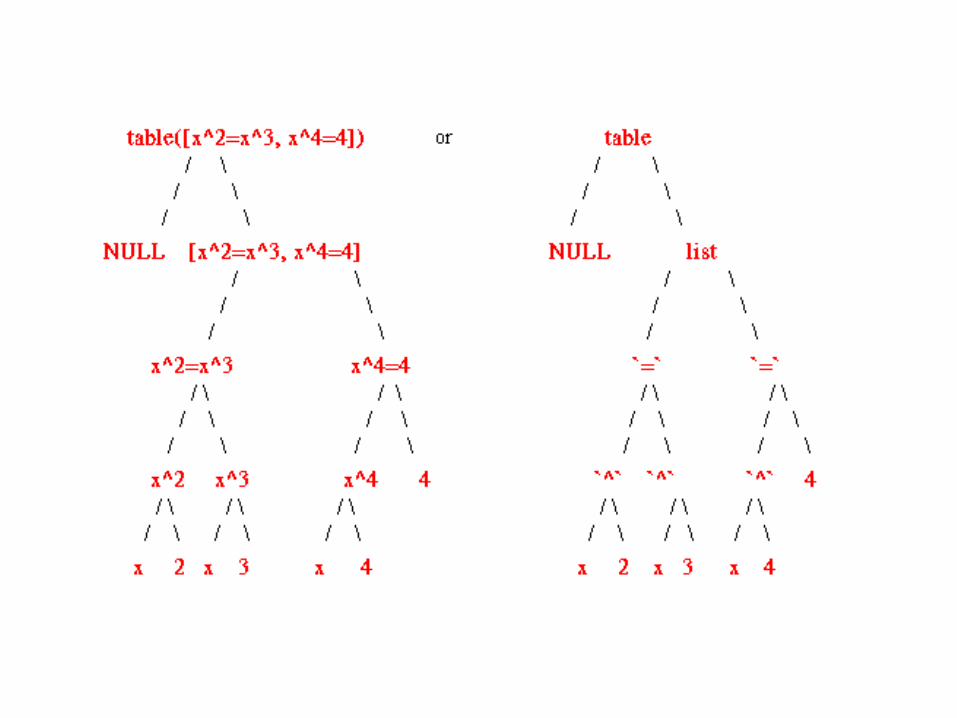
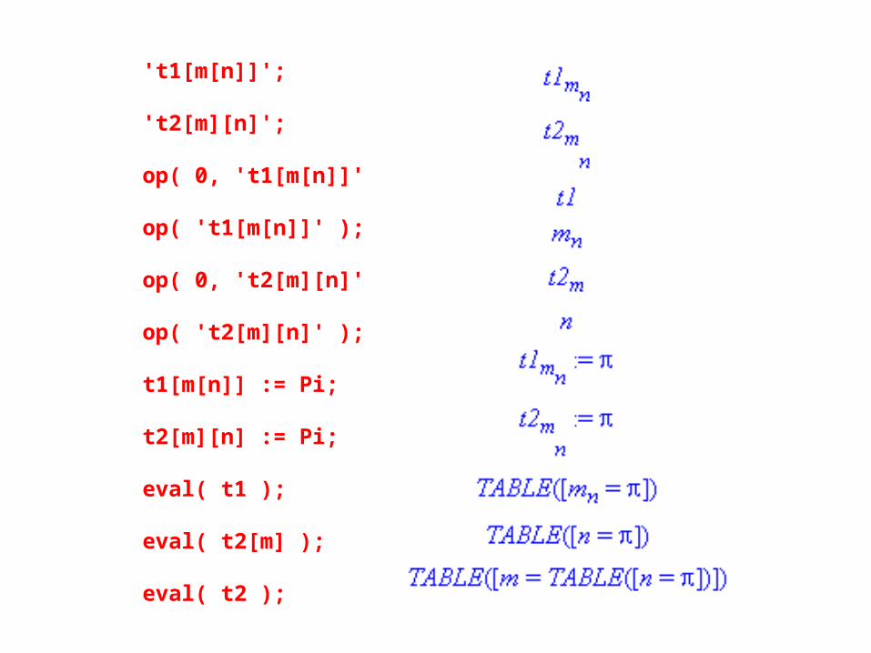
't1[m[n]]';

't2[m][n]';

op( 0, 't1[m[n]]' );

op( 't1[m[n]]' );

op( 0, 't2[m][n]' );

op( 't2[m][n]' );

t1[m[n]] := Pi;

t2[m][n] := Pi;

eval( t1 );

eval( t2[m] );

eval( t2 );

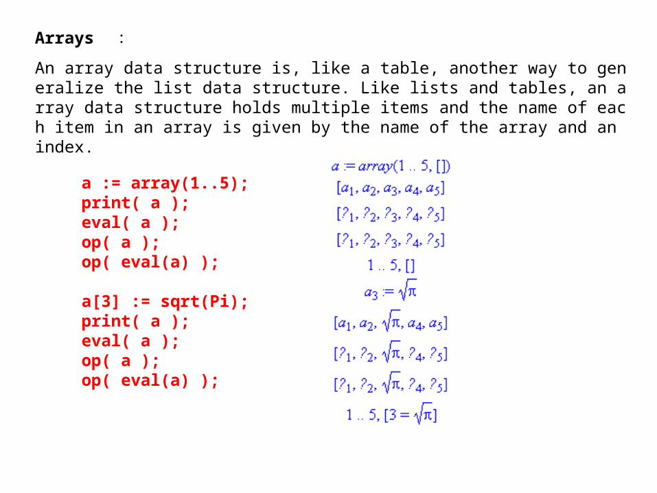
Arrays ：

An array data structure is, like a table, another way to generalize the list data structure. Like lists and tables, an array data structure holds multiple items and the name of each item in an array is given by the name of the array and an index.

a := array(1..5);print( a );eval( a );op( a );op( eval(a) );

a[3] := sqrt(Pi);print( a );eval( a );op( a );op( eval(a) );

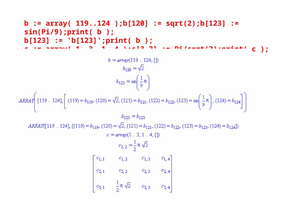
b := array( 119..124 );b[120] := sqrt(2);b[123] := sin(Pi/9);print( b );b[123] := 'b[123]';print( b );c := array( 1..3, 1..4 );c[3,2] := Pi/sqrt(2);print( c );

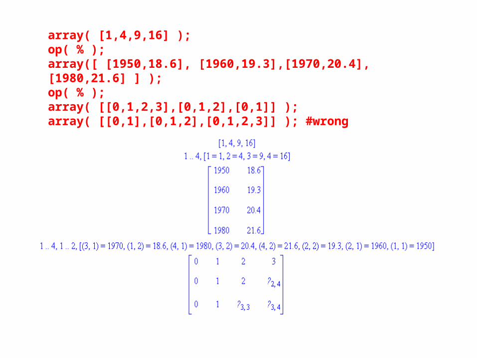
array( [1,4,9,16] );op( % );array([ [1950,18.6], [1960,19.3],[1970,20.4],[1980,21.6] ] );op( % );array( [[0,1,2,3],[0,1,2],[0,1]] );array( [[0,1],[0,1,2],[0,1,2,3]] ); #wrong

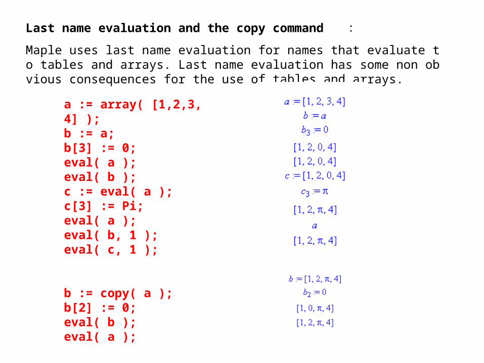
Last name evaluation and the copy command ：

Maple uses last name evaluation for names that evaluate to tables and arrays. Last name evaluation has some non obvious consequences for the use of tables and arrays.

a := array( [1,2,3,4] );b := a;b[3] := 0;eval( a );eval( b );c := eval( a );c[3] := Pi;eval( a );eval( b, 1 );eval( c, 1 );

b := copy( a );b[2] := 0;eval( b );eval( a );

a := array( 1..2, 1..2 );

a[1,1] := array( 1..2, 1..2 );

b := copy( a );

a[1,1][1,1] := 0;

print( a );

print( b );

a[2,1] := 5;

print( a );

print( b );

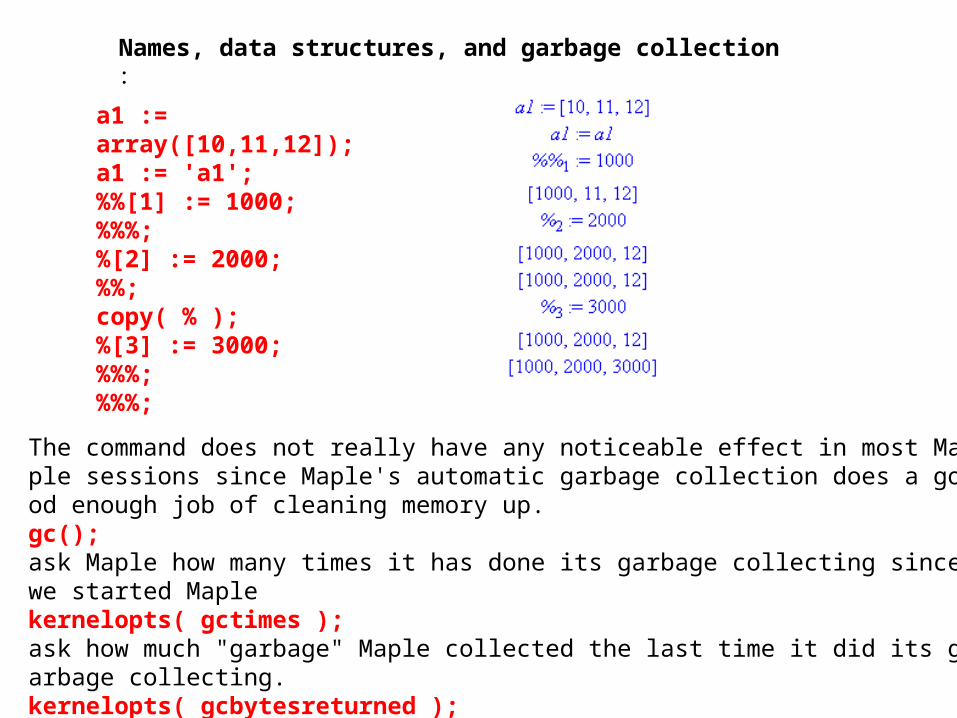
Names, data structures, and garbage collection ：

a1 := array([10,11,12]);a1 := 'a1';%%[1] := 1000;%%%;%[2] := 2000;%%;copy( % );%[3] := 3000;%%%;%%%;

The command does not really have any noticeable effect in most Maple sessions since Maple's automatic garbage collection does a good enough job of cleaning memory up.gc();ask Maple how many times it has done its garbage collecting since we started Maple kernelopts( gctimes );ask how much "garbage" Maple collected the last time it did its garbage collecting.kernelopts( gcbytesreturned );

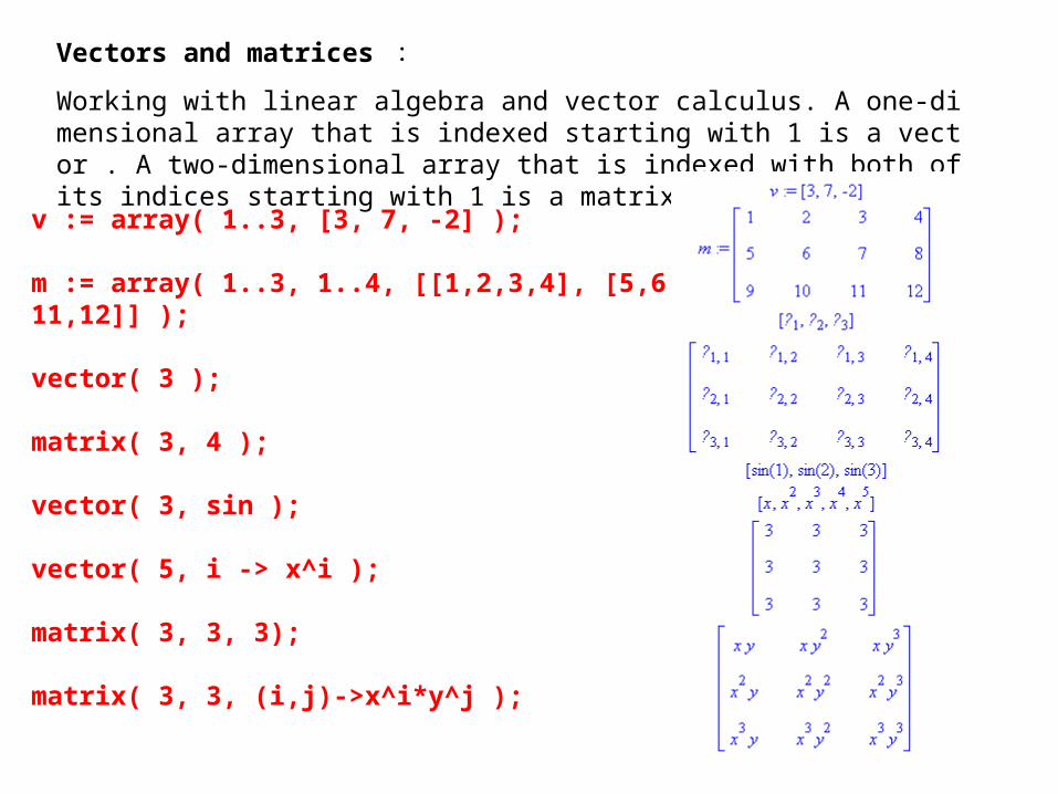
Vectors and matrices ：

Working with linear algebra and vector calculus. A one-dimensional array that is indexed starting with 1 is a vector . A two-dimensional array that is indexed with both of its indices starting with 1 is a matrix.

v := array( 1..3, [3, 7, -2] );

m := array( 1..3, 1..4, [[1,2,3,4], [5,6,7,8], [9,10,11,12]] );

vector( 3 );

matrix( 3, 4 );

vector( 3, sin );

vector( 5, i -> x^i );

matrix( 3, 3, 3);

matrix( 3, 3, (i,j)->x^i*y^j );

A := matrix( 2, 2, [1,2,3,4] );B := matrix( [[5,6], [7,8]] );evalm( A+B );evalm( A^2 );evalm( A*B ); #wrongevalm( A*B*A );evalm(A &* B &* A);

A := matrix( 2, 2, [1,2,3,4] );B := eval( A );C := copy( A );evalb( A=B );evalb( A=C );evalb( eval(A) = eval(B) );evalb( eval(A) = eval(C) );linalg[equal]( A, B );linalg[equal]( A, C );

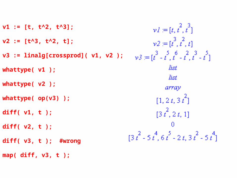
v1 := [t, t^2, t^3];

v2 := [t^3, t^2, t];

v3 := linalg[crossprod]( v1, v2 );

whattype( v1 );

whattype( v2 );

whattype( op(v3) );

diff( v1, t );

diff( v2, t );

diff( v3, t ); #wrong

map( diff, v3, t );

Index functions ：

An index function is a function associated to a table (or array) that allows the table (or array) to compute, rather than look up, the value associated to certain keys.

sym_t := table( symmetric );sym_t[a,b];sym_t[b,a];sym_t[4,2];sym_t[a,b] := 2;sym_t[b,a];op( sym_t );sym_t[b,a] := 12;op( sym_t );array( symmetric, 1..3, 1..3, [[5,6,7]] );array( antisymmetric, 1..3, 1..3 );

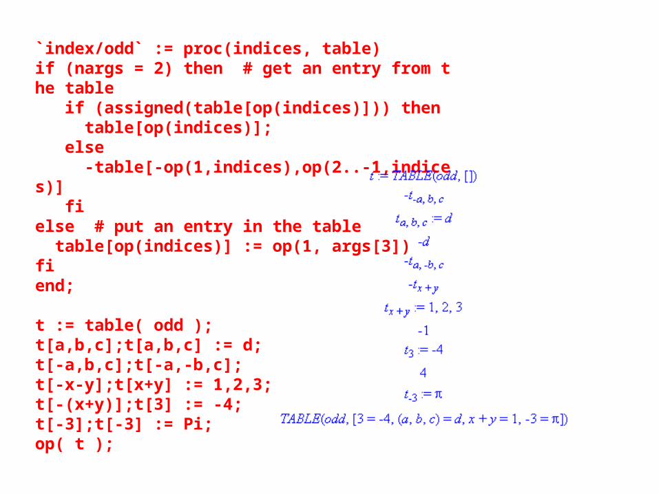
`index/odd` := proc(indices, table) if (nargs = 2) then # get an entry from the table if (assigned(table[op(indices)])) then table[op(indices)]; else -table[-op(1,indices),op(2..-1,indices)] fielse # put an entry in the table table[op(indices)] := op(1, args[3])fiend;

t := table( odd );t[a,b,c];t[a,b,c] := d;t[-a,b,c];t[-a,-b,c];t[-x-y];t[x+y] := 1,2,3;t[-(x+y)];t[3] := -4;t[-3];t[-3] := Pi;op( t );

Structured data types

Data types in general ：

type( 1/2, fraction );type( 0.5, float );type( 1/2, numeric );type( 0.5, numeric );type( 1/2, positive );type( 0.5, positive );type( 1/2, constant );type( 0.5, constant );whattype( 1/2 );whattype( 0.5 );s := 't';t := table();type( s, table );whattype( s );whattype( t );whattype( eval(s) );

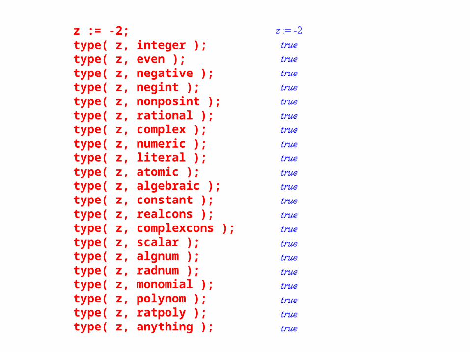
z := -2;type( z, integer );type( z, even );type( z, negative );type( z, negint );type( z, nonposint );type( z, rational );type( z, complex );type( z, numeric );type( z, literal );type( z, atomic );type( z, algebraic );type( z, constant );type( z, realcons );type( z, complexcons );type( z, scalar );type( z, algnum );type( z, radnum );type( z, monomial );type( z, polynom );type( z, ratpoly );type( z, anything );

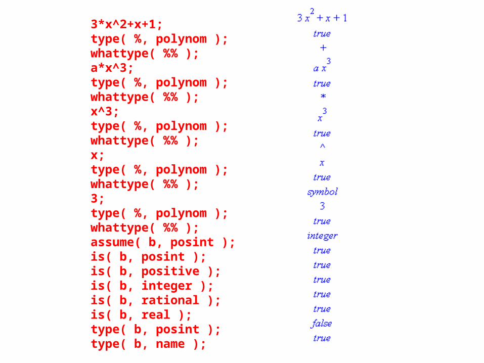
3*x^2+x+1;type( %, polynom );whattype( %% );a*x^3;type( %, polynom );whattype( %% );x^3;type( %, polynom );whattype( %% );x;type( %, polynom );whattype( %% );3;type( %, polynom );whattype( %% );assume( b, posint );is( b, posint );is( b, positive );is( b, integer );is( b, rational );is( b, real );type( b, posint );type( b, name );

posfrac_prop := AndProp(positive, fraction);assume( b, posfrac_prop );is( b, positive );is( b, fraction );is( b > 0 );about( b );is( 2/3, posfrac_prop );type( 2/3, posfrac_prop );posfrac_type := And(positive, fraction);type( 2/3, posfrac_type );assume( a, posfrac_type );is( a > -1 );is( a > 0 );about( a );smallfrac := AndProp(fraction, RealRange(Open(0), Open(2)));assume( b, smallfrac );is( b > 0 );is( b^2 < 4 );is( b, posfrac_prop );about( b );

Structured data types ：

Some data types describe the values in a data structure with more detail and precision than other data types. These more precise data types are called structured data types.

type( 5*x, numeric &* name );

type( x*y, numeric &* name );

type( x*y, name &* name );

type( 5*x*y, numeric &* name );

type( 5*x*y, `&*`(numeric,name,name) );

type( [1,2,3], list(integer) );

type( [u,v,w], list(symbol) );

type( [1/3, 3/5, 0.5], [fraction,fraction,float] );

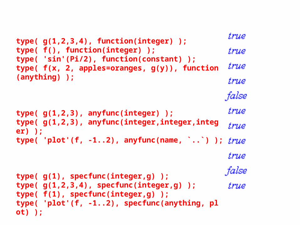
type( g(1,2,3,4), function(integer) );type( f(), function(integer) );type( 'sin'(Pi/2), function(constant) );type( f(x, 2, apples=oranges, g(y)), function(anything) );

type( g(1,2,3), anyfunc(integer) );type( g(1,2,3), anyfunc(integer,integer,integer) );type( 'plot'(f, -1..2), anyfunc(name, `..`) );

type( g(1), specfunc(integer,g) );type( g(1,2,3,4), specfunc(integer,g) );type( f(1), specfunc(integer,g) );type( 'plot'(f, -1..2), specfunc(anything, plot) );

type( x[1]+x[2]+y[0], `&+`(indexed) );

type( x[1]+x[2]+y[0], `&+`(indexed,indexed,indexed) );

type( 1/2*x*y[0], `&*`(fraction,symbol,indexed) );

type( 1/2, {fraction,name} );

type( x[0], {fraction,name} );

type( [1/2, x[0], y, 2/3], list({fraction,name}) );

type( 3*x, `&*`({numeric,name},name) );

type( a*x, `&*`({numeric,name},name) );

type( x^2-x-1=0, polynom=numeric );

b := 'a'; a := 0;

type( a, name(integer) );

type( 'a', name(integer) );

type( 'b', name(integer) );

type( 'b', name(name) );

type( 'b', name(name(integer)) );

type( 1/3, And(fraction, positive) );

type( -1/3, And(fraction, positive) );

type( 1/3, fraction and positive );

type( '1/3 and 10.5', fraction and positive );

type( '10.5 and 1/3', fraction and positive );

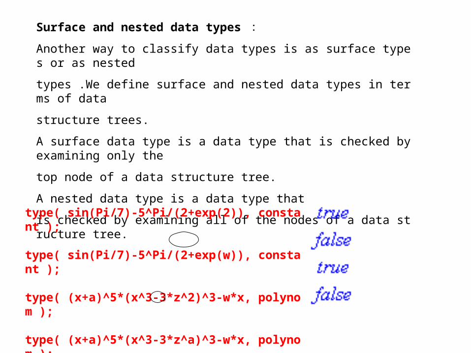
Surface and nested data types ：

Another way to classify data types is as surface types or as nested

types .We define surface and nested data types in terms of data

structure trees.

A surface data type is a data type that is checked by examining only the

top node of a data structure tree.

A nested data type is a data type that

is checked by examining all of the nodes of a data structure tree.

type( sin(Pi/7)-5^Pi/(2+exp(2)), constant );

type( sin(Pi/7)-5^Pi/(2+exp(w)), constant );

type( (x+a)^5*(x^3-3*z^2)^3-w*x, polynom );

type( (x+a)^5*(x^3-3*z^a)^3-w*x, polynom );

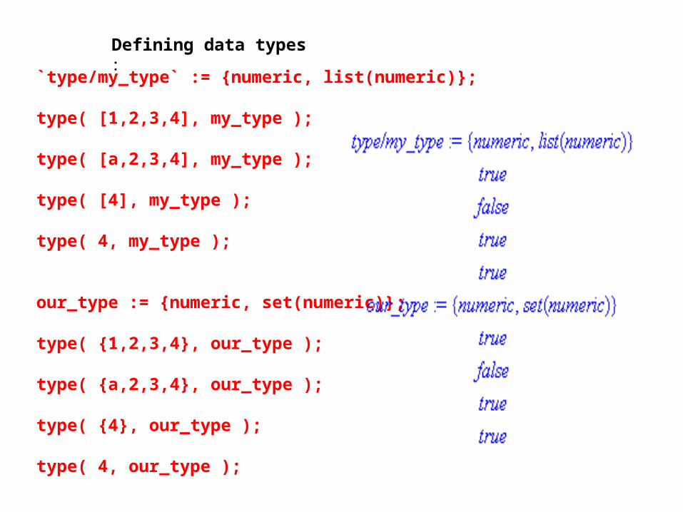
Defining data types ：

`type/my_type` := {numeric, list(numeric)};

type( [1,2,3,4], my_type );

type( [a,2,3,4], my_type );

type( [4], my_type );

type( 4, my_type );

our_type := {numeric, set(numeric)};

type( {1,2,3,4}, our_type );

type( {a,2,3,4}, our_type );

type( {4}, our_type );

type( 4, our_type );

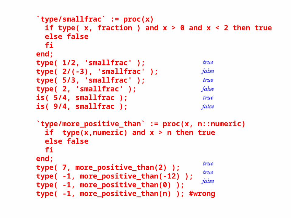
`type/smallfrac` := proc(x) if type( x, fraction ) and x > 0 and x < 2 then true else false fiend;type( 1/2, 'smallfrac' );type( 2/(-3), 'smallfrac' );type( 5/3, 'smallfrac' );type( 2, 'smallfrac' );is( 5/4, smallfrac );is( 9/4, smallfrac );

`type/more_positive_than` := proc(x, n::numeric) if type(x,numeric) and x > n then true else false fiend;type( 7, more_positive_than(2) );type( -1, more_positive_than(-12) );type( -1, more_positive_than(0) );type( -1, more_positive_than(n) ); #wrong