9772162243007 02 - scientific research...
TRANSCRIPT

9 772162 243007 20


Journal of Mathematical Finance, 2017, 7, 239-517 http://www.scirp.org/journal/jmf
ISSN Online: 2162-2442 ISSN Print: 2162-2434
Table of Contents Volume 7 Number 2 May 2017 The Economics of XVA Trading
P. J. Zeitsch……………………………………………………………………………………………………………239
A Comparison Study of ADI and LOD Methods on Option Pricing Models N. Bagheri, H. K. Haghighi……………………………………………………………………………………………275
Analysis of Cross-Correlations in Emerging Markets Using Random Matrix Theory T. C. Urama, P. O. Ezepue, C. P. Nnanwa……………………………………………………………………………291
Application of Fast N-Body Algorithm to Option Pricing under CGMY Model T. Sakuma……………………………………………………………………………………………………………308
Optimal Investment Strategy under Stochastic Interest Rates A. P. Mtunya, P. Ngare, Y. Nkansah-Gyekye…………………………………………………………………………319
Production Smoothing in Developed Countries I. Ginama, M. Odaki…………………………………………………………………………………………………333
Mathematical Analysis of Financial Model on Market Price with Stochastic Volatility M. K. Mondal, M. A. Alim, M. F. Rahman, M. H. A. Biswas………………………………………….……………351
An Empirical Evaluation in GARCH Volatility Modeling: Evidence from the Stockholm Stock Exchange
C. Dritsaki……………………………………………………………………………………………………………366
Foreign Direct Investment and Industrial Sector Performance: Assessing the Long-Run Implication on Economic Growth in Nigeria
E. S. Akpan, G. O. Eweke……………………………………………………………..………………………………391
Return Predictability and Strategic Trading under Symmetric Information M. Guo, H. Ou-Yang…………………………………………………………………..………………………………412
Commercial Bank Ownership Structure and Risk Preference H. X. Zhong…………………………………………………………………………..………………………………437
A Stochastic Correlation Model with Time Change for Pricing Credit Spread Options Z. G. Tong, A. Liu………………………………………………………………………..……………………………445
Jumps in High-Frequency Data on the Chinese Stock Market Y. Li, T. F. Jiang………………………………………………………………………..………………………………467
Journal of Mathematical Finance, 2017, 7, 239-517 http://www.scirp.org/journal/jmf
ISSN Online: 2162-2442 ISSN Print: 2162-2434
The Stochastic Volatility Model, Regime Switching and Value-at-Risk (VaR) in International Equity Markets
A. Assaf………………………………………………………………………………..………………………………491
Valuation of Derivatives on the Cost Variables of the Shipping Market C. E. Kountzakis………………………………………………………………………..……………………………513
The figure on the front cover is from the article published in Journal of Mathematical Finance, 2017, Vol. 7, No. 2, pp. 351-365 by Mitun Kumar Mondal, Md. Abdul Alim, Md. Faizur Rahman and Md. Haider Ali Biswas.

Journal of Mathematical Finance (JMF) Journal Information SUBSCRIPTIONS The Journal of Mathematical Finance (JMF) (Online at Scientific Research Publishing, www.SciRP.org) is published quarterly by Scientific Research Publishing, Inc., USA. Subscription rates: Print: $79 per issue. To subscribe, please contact Journals Subscriptions Department, E-mail: [email protected]
SERVICES Advertisements Advertisement Sales Department, E-mail: [email protected]
Reprints (minimum quantity 100 copies) Reprints Co-ordinator, Scientific Research Publishing, Inc., USA. E-mail: [email protected]
COPYRIGHT Copyright and reuse rights for the front matter of the journal: Copyright © 2017 by Scientific Research Publishing Inc. This work is licensed under the Creative Commons Attribution International License (CC BY). http://creativecommons.org/licenses/by/4.0/
Copyright for individual papers of the journal: Copyright © 2017 by author(s) and Scientific Research Publishing Inc.
Reuse rights for individual papers: Note: At SCIRP authors can choose between CC BY and CC BY-NC. Please consult each paper for its reuse rights.
Disclaimer of liability Statements and opinions expressed in the articles and communications are those of the individual contributors and not the statements and opinion of Scientific Research Publishing, Inc. We assume no responsibility or liability for any damage or injury to persons or property arising out of the use of any materials, instructions, methods or ideas contained herein. We expressly disclaim any implied warranties of merchantability or fitness for a particular purpose. If expert assistance is required, the services of a competent professional person should be sought.
PRODUCTION INFORMATION For manuscripts that have been accepted for publication, please contact: E-mail: [email protected]

Y. Li, T. F. Jiang
488
5. Conclusions
The findings of this study yield the following conclusions. First, the CSI 300 in-dex fundamentally involves a continuous-jump process, supporting the jump- diffusion model proposed by Mertaon (1976) [12]. Moreover, the activity indices of pure-jump models are inconsistent with any actual price processes and are therefore not representative of any active stock markets. In the price process of the Chinese stock market, the form of jump depends on continuous volatility processes; therefore, the analysis and expansion of pure-jump models are based on the Merton model. The CSI 300 index exhibits the characteristics of pure- jump or continuous processes in certain periods, making it necessary to adjust the price-volatility model for the index on the basis of macroeconomic factors and relevant policies.
Second, the continuous main-contract price process of the CSI 300 stock-in- dex futures agrees with continuous-martingale processes with jumps, indicating that continuous stochastic processes with jumps describe the volatility of stock- index futures markets. This may provide fresh insights into research on stock- index futures markets. Furthermore, in line with the CSI 300 index process, the continuous main-contract price process of the CSI 300 stock-index futures exhi-bits the characteristics of continuous-jump processes at most times and the cha-racteristics of pure-jump processes at certain times. Thus, the price process model for the CSI 300 stock-index futures should be adjusted depending on ac-tual circumstances.
Third, the volatility process of the CSI 300 index suggests that this process fits pure-jump processes more closely than it does other stochastic processes. This finding corresponds with those of Todorov and Tauchen that the VIX index is a pure-jump process. This contributes theoretically to the predication of the vola-tility of Chinese financial markets because parameterizing the time of volatility and fitting it with a pure-jump process may reflect the actual market volatility more closely.
Third, the analysis of cojumps suggests that jumps in the CSI 300 index price process and the continuous main-contract price process of the CSI 300 stock- index futures occur simultaneously in most cases (with a time lag of less than 5 minutes) and share a strong positive relationship. As such, the formulation of strategies on risk management and portfolio construction in the stock market or stock-index futures market in China should involve modeling the volatility of different markets. The price process of the Chinese stock market and the price volatility of the market show no notable cojump, although whether such a co-jump may ever occur during the development of the market necessitates further research.
Acknowledgements
This work was supported, in part, by the National Natural Science Foundation of China (Grant Nos. 70801066, 71071167, 71071168, 71371200), and by a grant

Y. Li, T. F. Jiang
489
from Sun Yat-sen University Basic Research Funding (Grant Nos. 1009028, 1109115, 16wkjc13).
References [1] Todorov, V. and Tauchen, G. (2010) Activity Signature Functions for High-Fre-
quency Data Analysis. Journal of Econometrics, 154, 125-138.
[2] Jacod, J. and Todorov, V. (2009) Testing for Common Arrivals of Jumps for Dis-cretely Observed Multi-Dimensional Processes. Annals of Statistics, 37, 1792-1838. https://doi.org/10.1214/08-AOS624
[3] Liu, J. and Pan, J. (2003) Dynamic Derivative Strategies. Journal of Financial Eco-nomics, 69, 401-430.
[4] Bollerslev, T., Law, T. and Tauchen, G. (2008) Risk, Jumps, and Diversification. Journal of Econometrics, 144, 234-256.
[5] Cont, R. and Tankov, P. (2003) Financial Modelling with Jump Processes. Chapman and Hall, Boca Raton, Florida. https://doi.org/10.1201/9780203485217
[6] Heston, S. (1993) A Closed-Form Solution for Options with Stochastic Volatility with Applications to Bond and Currency Options. Review of Financial Studies, 6, 327-343. https://doi.org/10.1093/rfs/6.2.327
[7] Eraker, B., Johannes, M. and Polson, N. (2003) The Impact of Jumps in Volatility and Returns. Journal of Finance, 58, 1269-1300. https://doi.org/10.1111/1540-6261.00566
[8] Wu, L. (2011) Variance Dynamics: Joint Evidence from Options and High-Fre- quency Returns. Journal of Econometrics, 160, 280-287.
[9] Geman, H. (2003) Pure Jump Levy Processes for Asset Price Modeling. EFA 2003 Annual Conference Paper No. 590.
[10] Barndorff-Nielsen, O. and Shephard, N. (2001) Non-Gaussian Ornstein-Uhlenbeck- Based Models and Some of Their Uses in Financial Economics. Journal of the Royal Statistical Society Series B, 63, 167-241. https://doi.org/10.1111/1467-9868.00282
[11] Fama, E.F. (1965) The Behavior of Stock-Market Prices. Journal of Business, 38, 34-105. https://doi.org/10.1086/294743
[12] Merton, R. (1976) Option Pricing When the Underlying Stock Returns Are Discon-tinuous. Journal of Financial Economics, 3, 125-144.
[13] Duffie, D., Pan, J. and Singleton, K. (2000) Transform Analysis and Asset Pricing for Affine Jump-Diffusions. Econometrica, 68, 1343-1376. https://doi.org/10.1111/1468-0262.00164
[14] Nelson, D.B. (1991) Conditional Heteroskedasticity in Asset Returns: A New Ap-proach. Econometrica, 59, 347-370. https://doi.org/10.2307/2938260
[15] Whaley, R.E. (1993) Derivatives on Market Volatility: Hedging Tools Long Over-due. Journal of Derivatives, 1, 71-84. https://doi.org/10.3905/jod.1993.407868
[16] Huang, X. and Tauchen, G. (2005) The Relative Contribution of Jumps to Total Price Variance. Journal of Financial Econometrics, 3, 456-499. https://doi.org/10.1093/jjfinec/nbi025
[17] Ait-Sahalia, Y. and Jacod, J. (2009) Estimating the Degree of Activity of Jumps in High Frequency Data. Annals of Statistics, 37, 2202-2244. https://doi.org/10.1214/08-AOS640
[18] Ait-Sahalia, Y. and Jacod, J. (2009) Testing for Jumps in a Discretely Observed Process. Annals of Statistics, 37, 184-222. https://doi.org/10.1214/07-AOS568

Y. Li, T. F. Jiang
490
[19] Cao, H.D., Li, Y. and He, Z. (2011) Stock Pricing Model: Jump Diffusion Model of Power Law. Journal of Management Sciences in China, 14, 46-59.
[20] Chen, G.J. and Wang, Z.H. (2010) Continuous Volatility and Jump Volatility in China’s Stock Market. System Engineering Theory and Practice, 30, 1554-1562.
[21] Gilder, D. (2009) An Empirical Investigation of Intraday Jumps and Cojumps in US Equities. Research Paper. http://citeseerx.ist.psu.edu/viewdoc/download?doi=10.1.1.503.9736&rep=rep1&type=pdf
[22] Dungey, M. and Hvozdyk, L. (2012) Cojumping: Evidence from the US Treasury Bond and Futures Markets. Journal of Banking & Finance, 36, 1563-1575.
[23] Forbes, K.J. and Rigobon, R. (2002) No Contagion, Only Interdependence: Mea-suring Stock Market Comovements. Journal of Finance, 57, 2223-2261. https://doi.org/10.1111/0022-1082.00494
[24] Delbaen, F. and Schachermayer, W. (1994) A General Version of the Fundamental Theorem of Asset Pricing. Mathematische Annalen, 300, 463-520. https://doi.org/10.1007/bf01450498
[25] Blumenthal, R. and Getoor, R. (1961) Sample Functions of Stochastic Processes with Independent Increments. Journal of Mathematics and Mechanics, 10, 493-516.
[26] Ait-Sahalia, Y. and Jacod, J. (2007) Volatility Estimators for Discretely Sampled Levy Processes. Annals of Statistics, 35, 355-392. https://doi.org/10.1214/009053606000001190
[27] Barndorff-Nielsen, O. and Shephard, N. (2003) Realized Power Variation and Sto-chastic Volatility Models. Bernoulli, 9, 243-265. https://doi.org/10.3150/bj/1068128977
[28] Jacod, J. and Shiryaev, A.N. (2003) Limit Theorems for Stochastic Processes. 2nd Edition, Springer Verlag, Berlin. https://doi.org/10.1007/978-3-662-05265-5
[29] Corcuera, J., Nualart, D. and Woerner, J. (2006) Power Variation of Some Integral Fractional Processes. Bernoulli, 12, 713-735. https://doi.org/10.3150/bj/1155735933
Submit or recommend next manuscript to SCIRP and we will provide best service for you:
Accepting pre-submission inquiries through Email, Facebook, LinkedIn, Twitter, etc. A wide selection of journals (inclusive of 9 subjects, more than 200 journals) Providing 24-hour high-quality service User-friendly online submission system Fair and swift peer-review system Efficient typesetting and proofreading procedure Display of the result of downloads and visits, as well as the number of cited articles Maximum dissemination of your research work
Submit your manuscript at: http://papersubmission.scirp.org/ Or contact [email protected]

Journal of Mathematical Finance, 2017, 7, 491-512 http://www.scirp.org/journal/jmf
ISSN Online: 2162-2442 ISSN Print: 2162-2434
DOI: 10.4236/jmf.2017.72026 May 31, 2017
The Stochastic Volatility Model, Regime Switching and Value-at-Risk (VaR) in International Equity Markets
Ata Assaf
Faculty of Business Administration, University of Balamand, Balamand, Lebanon
Abstract In this paper, we estimate two stochastic volatility models applied to interna-tional equity markets. The two models are the log-normal stochastic volatility (SV) model and the two-regime switching model. Then based on the one-day- ahead forecasted volatility from each model, we calculate the Value-at-Risk (VaR) in each market. The estimated VaR measures from the SV are higher than those obtained from the regime-switching model for all markets and over all horizons. The exception is the Japanese market, where the stochastic volatility model generates low VaR estimates. Comparing those estimates with the unconditional return distribution, the two models generate smaller VaR measures; an evidence of the two models capturing volatility changes in in-ternational equity markets. Finally, we backtest each model and find that the performance of both models is the worst for the Canadian stock market, while the regime switching model does poorly for Germany. The results have signif-icant implications for risk management, trading and hedging activities as well as in the pricing of equity derivatives.
Keywords Regime Switching, Stochastic Volatility Model, Value at Risk
1. Introduction
Volatility is a key ingredient for derivative pricing, portfolio optimization and value-at-risk analysis. Hence, accurate estimates and good modeling of stock price volatility are of central interest in financial applications. The valuation of financial instruments is complicated by two characteristics of the volatility process. First, it is generally acknowledged that the volatility of many financial return series is not constant over time and exhibits prolonged periods of high
How to cite this paper: Assaf, A. (2017) The Stochastic Volatility Model, Regime Switching and Value-at-Risk (VaR) in International Equity Markets. Journal of Mathematical Finance, 7, 491-512. https://doi.org/10.4236/jmf.2017.72026 Received: March 8, 2017 Accepted: May 24, 2017 Published: May 31, 2017 Copyright © 2017 by author and Scientific Research Publishing Inc. This work is licensed under the Creative Commons Attribution International License (CC BY 4.0). http://creativecommons.org/licenses/by/4.0/
Open Access
A. Assaf
492
and low volatility, often referred to as volatility clustering [1] [2]. Second, vola-tility is not directly observable1. Two models have been developed which capture this time-varying autocorrelated volatility process: the GARCH and the Stochas-tic Volatility (SV) model. GARCH models define the time-varying variance as a deterministic function of past squared innovations and lagged conditional va-riances whereas the variance in the Stochastic Volatility model is modeled as an unobserved component that follows some stochastic process. Stochastic volatility models are also attractive because they are close to the models often used in fi-nancial theory to represent the behavior of financial prices. Furthermore, their statistical properties are easy to derive using well-known results on log-normal distributions. Finally, compared with the more popular GARCH models, they capture the main empirical properties often observed in daily series of financial returns (see, for example, Carnero et al., [23]). For surveys on the extensive GARCH literature we refer to Bollerslev et al. [5], Bera and Higgins [6] and Bol-lerslev et al. [7] and for stochastic volatility we refer to Taylor [8], Ghysels et al. [9] Shephard [10], and Broto and Ruiz [11]. Both models are defined by their first and second moments. The Stochastic Volatility model introduced by Taylor [8] provides an alternative to the GARCH model in accounting for the time- varying and persistent volatility as well as for the leptokurtosis in financial re-turn series. The stochastic volatility models present two main advantages over ARCH models. The first one is their solid theoretical background, as they can be interpreted as discretized versions of stochastic volatility continuous-time mod-els put forward by modern finance theory (see Hull and White [12]). The second is their ability to generalize from univariate to multivariate series, as far as their estimation and interpretation are concerned. On the other hand, stochastic vola-tility models are more difficult to estimate than ARCH models, due to the fact that it is not easy to derive their exact likelihood function. For this reason, a number of econometric methods have been proposed to solve the problem of es-timation of stochastic volatility models.
The stochastic volatility model defines volatility as a logarithmic first-order autoregressive process. It is an alternative to the GARCH models which have re-lied on simultaneous modeling of the first and second moment. For certain fi-nancial time series such as stock index return, which have been shown to display high positive first-order autocorrelations, this constitutes an improvement in terms of efficiency; see Campbell et al. [13]. The volatility of daily stock index returns has been estimated with stochastic volatility models but usually results have relied on extensive pre-modeling of these series, thus avoiding the problem of simultaneous estimation of the mean and variance. Koopman and Hol Us-pensky [14] proposed the Stochastic Volatility in Mean model (SVM) that in- corporates volatility as one of the determinants of the mean. This modification makes the model suitable for empirical applications between the mean and va-riance of returns. The SVM model can be viewed as the SV counterpart of the
1For a comprehensive review of volatility measures and their properties see Andersen, Bollerslev and Diebold [3] and for forecasting financial volatility see the survey by Poon and Granger [4].
A. Assaf
493
ARCH-M model of Engle et al. [2] with the main difference between the two models is that the ARCH-M model intends to estimate the relationship between expected returns and expected volatility, whereas the aim of the SVM model is to simultaneously estimate the ex ante relation between returns and volatility and the volatility feedback effect.
Another way of modeling financial time series is to define different states of the world or regimes, and to allow for the possibility that the dynamic behavior of financial variables to depend on the regime that occurs at any given point in time. That means that certain properties of the time series, such as its mean, va-riance and/or autocorrelation, are different in different regimes. Regime switch-ing models were first introduced by Goldfeld and Quandt [15] to provide a sim-ple way to model endogenously determined structural breaks or regime shifts in parameters. Hamilton [16] generalizes this setting by allowing the mixing prob-ability to be time-varying function of the history of the data. To illustrate the importance of stochastic regime switching for financial time series, for example, LeBaron [18] shows that the autocorrelations of stock returns are related to the level of volatility of these returns. In particular, autocorrelations tend to be larger during periods of low volatility and smaller during periods of high volatility. The periods of low and high volatility can be interpreted as distinct regime—or, put differently, the level of volatility can be regarded as the regime-determining process. In this setup, the level of volatility is not known with certainty and what we can do is to make a sensible forecast of this level, and hence, of the regimes that will occur in the future, by assigning probabilities to the occurrence of the different regimes.
Markov switching models have been found to provide a flexible framework to handle many features of asset returns. In particular, they allow for nonlinearities arising from persistent jumps in the model parameters and have several appeal-ing features. First, they provide a convenient framework to endogenously iden-tify regime shifts that are commonplace in financial data. Regimes are treated as latent processes which are not observable, but can be inferred from the estima-tion algorithm using observable data, such as the history of the asset’s returns. Second, as Markov switching models belong to the mixture-of-distributions class of stochastic processes, they are as versatile as mixture models in capturing sa-lient features of financial data such as time-varying volatilities, skewness, and leptorkurtosis. A detailed study of the statistical properties of Markov switching models by Timmerman [18] shows the Markov switching models can indeed approximate general classes of density functions with a wide range of condition-al moments. Ang and Bekaert [19] show that Markov switching models with state-dependent means and variances can match exceedance correlations better than do standard GARCH models or bivariate jump diffusion processes.
Related to the two models, returns on equity markets were also found to be characterized by jumps, and these jumps tend to occur at the same time across countries, implying that conditional correlations between international equity returns tend to be higher in periods of high market volatility or following large

A. Assaf
494
downside moves. Evidence on jumps is provided by Jorion [20], Akgiray and Booth [21], Bates [22], and Bekaert et al. [23], and Asgharian and Bengtsson [24]2. For example, Asgharian and Bengtsson [24] studied the jump spillover between equity indexes using a Bayesian approach and found the probabilities that jumps in large countries cause jumps or large returns in other countries. They also found significant evidence of jump spillover, particularly large be-tween countries that belong to the same regions and have similar industry structure3.
In this paper, we extend on the existing literature by modeling the interna-tional equity markets according to two volatility models: the log-normal SV model and the two-regime switching model. The log-normal SV model will be is estimated by quasi-maximum likelihood with the kalman filter while the two- regime switching model will be estimated by maximum likelihood with the Hamilton filter. The results provide new evidence on the dynamics of risk and return in equity markets with the possible existence of regimes in these markets. Then based on the one-day-ahead forecasted conditional volatility from each model, we calculate the one day Value-at-Risk (VaR). Then, we backtest those results from each model using unconditional and conditional tests. We find that the value at risk estimates are higher for the SV model than those obtained un-der the regime-switching model for all markets and over all horizons. The ex-ception is for the Japanese market. The stochastic volatility model generates lower VaR values than those of the regime switching model. A characteristic that reflects the performance of the Japanese market during the sample period, when Japan was hit by a real estate bubble and a banking crisis that made the volatility in that market lower than those observed in other markets. Then, considering the value at risk measures obtained directly from the two models and comparing them to those obtained from the unconditional return distribution, the two models provide smaller value at risk measures. Finally, comparing how the Val-ue-at-Risk behaves with the time horizon, value at risk measures increase more slowly with horizon under the regime switching model than those obtained un-der the stochastic volatility model4. The performance of both models are then backtested using conditional and unconditional tests and we find that the Cana-dian equity market represented by the S & P/TSX performs the worst among all markets, while the DAX seems to be better modeled by the stochastic volatility model as opposed to that of the regime switching model.
Our results deviate from those obtained by the above mentioned literature in the following aspects: 1) the sample size is longer than previously studied; 2) the previous literature either focuses on one single market or few (i.e, Kuester et al. [31]) we provide a forecasted one day ahead volatility based on each model and
2For evidence on changing conditional correlations see, for instance Ang and Chen [25], Longin and Solnik [26], Karolyi and Stulz [27], and Chakrabarti and Roll [28]. 3Other studies using copula functions were used to study diversification benefits and dependence between American and developed markets as done by Chollete et al. [29], and Buraschi et al. [30]. 4Our result fall in line of those conducted by Kuester et al. [31]. Yet their study is made only on the NASDAQ, while ours cover more markets and a larger sample period.

A. Assaf
495
consequently use that to calculate value at risk measures; and finally 4) we find that the Canadian and Japanese markets appear to have different features than those obtained in previous results, whether in terms of the risk measures ob-tained by the two models or in terms of the suitability of each model when we backtest them.
The paper is organized as follows. Section 2 introduces the two models: the regime switching model and the stochastic volatility model. Section 3 describes the available data and presents the stylized facts of the corresponding realized volatility. Section 4 presents the estimation results from the two models. Section 5 provides the Value at Risk measures and backtesting results. Section 5 con-cludes.
2. Models of Volatility
The empirical regularities of asset returns (i.e., volatility clustering; squared re-turns exhibit prolonged serial correlation; and heavy tails and persistence of vo-latility) suggest that the behavior of financial time series can be captured by a model which recognizes the time-varying nature of return volatility as follows:
t t t ty µ σ ε= + (1)
,11
k
t i ii
a b xµ=
= +∑ (2)
with tε follows NID(0, 1). tµ represents the mean and depends on a constant a and regression coefficients 1, , kb b . The explanatory variables 1, ,, ,t k tx x
may also contain lagged exogenous and dependent variables. The disturbance term tε is IID with zero mean and unit variance and a usual assumption of a normal distribution.
Following Shephard [10], models of changing volatility can be usefully parti-tioned into observation-driven and parameter-driven models and both can be expressed using a parametric framework as: t ty z follows a ( )2,t tN µ σ . In the first class, the autoregressive heteroskedasticity (ARCH) models introduced by Engle [32] are the most representative example. In the second class, tz is a function of an unobserved or latent component. The log-normal stochastic vola-tility model created by Taylor [8] is the simplest and best known example:
1t t th hα β η−= + + (3)
with t ty z following a N(0, exp(ht)) and ηt being ( )20,NID ησ . Where ht represents the log-volatility, which is unobserved but can be esti-
mated using the observations. One interpretation for the latent ht is to represent the random and uneven flow of new information, which is difficult to model di-rectly, into financial markets. The most popular model from Taylor [8], puts
( )exp 2t t ty hε= and 1t t th hα β η−= + + (4)
where εt and ηt are two independent Gaussian white noises, with variances 1 and 2ησ , respectively. Due to the Gaussianity of ηt, this model is called a log-normal
SV model. Although the assumption of Gaussianity of ηt can seem ad hoc at first

A. Assaf
496
sight, Andersen et al. [33] [34] show that the log-volatility process can be well approximated by a Normal distribution.
Another possible interpretation for ht is to characterize the regime in which financial markets are operating and then it could be described by a discrete va-lued variable. The most popular approach to modelling changes in regime is the class of Markov switching models introduced by Hamilton [16]. In that case the model is where ( )exp 2t t ty hε= and t th sα β= + where st is a two state first- order Markov chain which can take values 0, 1 and is independent of εt. The value of the time series st, for all t, depends only on the last value st−1 for i, j = 0, 1:
( ) ( )1 2 1| , , |t t t t t ijP s j s i s i P s j s i p− − −= = = = = = = (5)
The probabilities ( ) , 0,1ij i jp
= are called transition probabilities of moving
from one state to the other. These transition probabilities are collected in the transition matrix P:
00 11
00 11
11
p pp p
− −
(6)
which fully describes the Markov chain and also we get: 00 01 10 11 1p p p p+ = + = . A two-state Markov chain can be represented by a simple AR(1) process as fol-lows:
( ) ( )00 00 11 11 1t t ts p p p s υ−= − + − + + + (7)
where ( )1 2 ,| ,t t t t ts E s s sυ − −= − and the volatility equation can be written the following way:
( ) ( )00 00 11 11 1t t t th s p p p sα β α β υ− = + = + − + − + + + (8)
or
( ) ( ) ( )00 11 00 00 11 1
1
2 1 1t t t
t t
h p p p p p ha bh
β βυϖ
−
−
= − − + − + − + + +
= + + (9)
which implies the same structure of the stochastic volatility model but with a noise that can take only a finite set of values.
3. Estimation Methods
A variety of estimation procedures has been proposed for the stochastic volatility models, including for example the Generalized Method of Moments (GMM) used by Melino and Turnbull [35], the Quasi Maximum Likelihood (QML) ap-proach followed by Harvey et al. [36] and Ruiz [37], the Efficient Method of Moments (EMM) applied by Gallant et al. [38], and Markov-Chain Monte Carlo (MCMC) procedures used by Jacquier et al. [39] and Kim et al. [40]. In this pa-per, the parameters of the SV model are estimated by the exact maximum like-lihood method using Monte Carlo importance sampling techniques. We refer the reader to Koopman and Hol Uspensky [14] for more explanation. The like-

A. Assaf
497
lihood function for the SV model can be constructed using simulation methods developed by Shephard and Pitt [41] and Durbin and Koopman [42]. For the SV model we can express the likelihood function as:
( ) ( ) ( ) ( ) ( ), d , dL p y p y p y pψ ψ θ ψ θ θ ψ θ ψ θ= = =∫ ∫ (10)
where ( ), ,η εψ ϕ σ σ= ′ , ( )1, , Th hθ = ′ . An efficient way of evaluating such ex-
pressions is by using importance sampling; see Ripley [43], Chapter 5). A simu-lation device is required to sample from an importance density ( ),p y θ ψ which is preferred to be as close as possible to the true density ( ),p y θ ψ . A choice for the importance density is the conditional Gaussian density since in this case it is relatively straightforward to sample from ( ) ( ), ,p y g yθ ψ θ ψ= using simulation smoothers such as the ones developed by de Jong and Shephard [44] and Durbin and Koopman [42]. All models were estimated using programs written in the Ox language of Doornik [45] using SsfPack by Koopman, She- phard and Doornik [46]. The log-normal SV model which is estimated by qua-si-maximum likelihood with the kalman filter, and the two-regime switching model which is estimated by maximum likelihood with the Hamilton filter. The Ox programs were downloaded from http://personal.vu.nl/s.j.koopman/SJresearch.html.
The log-normal SV model is represented by Equation (4) with εt and ηt inde-pendent Gaussian white noises. Their variances are 1 and 2
ησ , respectively. The volatility equation is characterized by the constant parameter α, the autoregres-sive parameter β and the variance 2
ησ of the volatility noise. The mean is either imposed equal to zero or estimated with the empirical mean of the series. Since the specification of the conditional volatility is an autoregressive process of order one, the stationarity condition is |β| < 1. Moreover, the volatility ση must be strictly positive. In the estimation procedure the following logistic and logarithm reparameterizations:
( )( )
exp2 1
1 expb
bβ
= − +
and ( )expn sησ = (11)
have been considered in order to satisfy these conditions. The second model is a particular specification of the regime switching model
introduced by Hamilton, with the distribution of the returns is described by two regimes with the same mean but different variances and by a constant transition matrix:
0
1
if 0if 1
t tt
t t
sy
sµ σ εµ σ ε+ =
= + = (12)
and
00 11
00 11
11
p pp p
− −
where st is a two-state Markov chain independent of εt, which is a Gaussian white noise with unit variance. The parameters of this model are the mean μ, the low and high standard deviation σ0, σ1 and the transition probabilities p00, p11
A. Assaf
498
(also called regime transformations probabilities). As for the log-normal SV model, the logarithm and the logistic transformations ensure the positiveness of the volatilities and constrain the transition probabilities to assume values in the (0, 1) interval. Further, for the log-normal SV model the returns are modified as follows: ( )* log 1.27t t ty y y= − + where ty is the empirical mean. Thus, for the log-normal SV model the mean is not estimated but is simply set equal to the empirical mean. For the estimation, the starting values of the parameters are calculated considering the time series analyzed. For example, the sample mean is used as an approximation of the mean of the switching regime model and the empirical variance multiplied by appropriate factors is used for the high and low variance. However, for the log-normal SV model, a range of possible values of the parameters were fixed and a value is randomly extracted.
4. Estimation Results
We examine the behavior of the following equity markets. These are the S & P500 for USA, FTSE100 for United Kingdom, CAC40 for France, S & P/TSX for Canada, Nikkei225 for Japan, DAX for Germany, and Swiss Market for Switzer-land. We use a sample from 11/4/1996 to 12/10/2008 resulting in 3158 data points. The price data was obtained from Datastream. Each of the price indices was transformed via first differencing of the log price data to create a series, which approximates the continuously compounded percentage return. The stock index prices are not adjusted for dividends following studies of French et al. [47] and Poon and Taylor [48] who found that inclusion of dividends affected esti-mation results only marginally. Returns are calculated on a continuously com-pounded basis and expressed in percentages, they are therefore calculated as
( )( )1100 logt t tr P P−= ∗ , where Pt denotes the stock index in day t. The summary statistics are presented in Table 1. We observe that the Swiss
Market shows the highest mean returns followed by CAC40 and then the DAX. All the indices exhibit similar patterns of volatility represented by the standard deviation, with Nikkei225 having the highest variability and S & P/TSX having the lowest. We further observe that the returns are highly autocorrelated at lag 1, with S & P/TSX maintaining the highest autocorrelation. The high first-order autocorrelation reflects the effects of non-synchronous or thin trading, whereas highly correlated squared returns can be seen as an indication of volatility clus-tering. The Q(12) and Qs(12) test statistics, which is a joint test for the hypothe-sis that the first twelve autocorrelation coefficients on returns and squared re-turns are equal to zero, indicate that this hypothesis has to be rejected at the 1% significance level for all return series and squared return series. A number of empirical studies has found similar results on market returns distributional cha-racteristics. Kim and Kon [49] showed similar results for 30 stocks in DJIA, S & P500, and CRSP indices. Campbell, Lo and Mackinlay [13] concluded that daily US stock indexes show negatively skewed and positive excess kurtosis. The au-tocorrelation of squared returns is consistent also with the presence of time- varying volatility such as GARCH effects. As pointed out by Lamoureux and

A. Assaf
499
Table 1. Summary statistics of daily returns.
S & P500 FTSE100 NIKKEI225 DAX S & P/TSX CAC40 SM
Mean −0.0089 0.017 −0.026 0.020 −0.007 0.029 0.037
S.D 1.008 1.089 1.495 1.080 0.745 1.002 1.200
Skewness −0.205 −0.069 0.123 −0.506 −0.632 0.358 −0.237
Kurtosis 7.538 5.684 5.051 8.248 9.174 6.448 7.486
J.B. 2731* 950* 561* 3757* 5225* 1631* 2678*
ρ₁ ρ₂ ρ₃
0.052 0.005 0.064
0.020 −0.041 −0.085
−0.028 −0.050 0.018
0.078 −0.013 −0.016
0.117 −0.012 0.019
0.074 0.040
−0.024
0.051 −0.004 −0.041
Q(12) 60.04* 59.04* 15.87* 72.17* 87.72* 87.41* 29.57*
ρs1
ρs2 ρs3
0.182 0.244 0.191
0.214 0.302 0.255
0.099 0.123 0.153
0.107 0.165 0.160
0.129 0.173 0.110
0.165 0.188 0.141
0.232 0.268 0.212
Qs(12) 1186* 2173* 373* 796* 687* 113* 1691*
The table contains summary statistics for the international equity markets. J.B. is the Jarque-Bera normality test statistic with 2 degrees of freedom; ρk is the sample autocorrelation coefficient at lag k with asymptotic
standard error 1 T and Q(k) is the Box-Ljung portmanteau statistic based on k-squared autocorrela-tions. ρsk are the sample autocorrelation coefficients at lag k for squared returns and Qs(12) is the Box-Ljung portmanteau statistic based on 12-squared autocorrelations. * indicates significance at 99%. ** indicates significance at 95%. *** indicates significance at 90%.
Lastrapes [50] and confirmed by Hamilton and Susmel [51], regime shifts in the volatility process can also induce a spuriously high degree of volatility cluster-ing5.
The estimation results of the two models are reported in Table 2 and Table 3. Table 2 presents the results of estimating the regime switching model in the dif-ferent markets. For this model, we can judge the persistence of the volatility from the values taken by the transition (or persistence) probabilities p00 and p11, they are all high and higher than 0.90, confirming the high persistence of the vo-latility in all markets. The parameter which govern the mean process is also re-ported in the first column of Table 2 with the corresponding standard errors. The mean parameter is positive and statistically significant for all series, except being negative for Nikkei225. The Japanese market is the exception since it had gone through major structural changes during the sample period, in terms of its risk and return characteristics. The estimation results of the log-normal SV model are reported in Table 3. For this model, the standard errors are calculated following Ruiz [37] for the log-normal SV model and as the inverse of the in-formation matrix for the switching model. In both cases the z-statistics asymp-totically follow an N(0, 1) distribution. All markets show strong persistence, since all the estimated autoregressive coefficients of the volatility equation (β) are higher than 0.90. Also all the volatility estimates are all highly significant and
5Before estimating the models, we test whether there are indeed regime shifts in the stock markets and whether a stochastic volatility model fits the data well. To do so, we apply Hansen’s [52] mod-ified likelihood ratio test for regimes and Kobayashi and Shi [53] tests. Results are available upon request.

A. Assaf
500
Table 2. Results of the regime switching model applied to international equity markets.
Stock index μ Low Persis. Pr. High Persis. Pr. LowV High V FV LogL
S & P500 0.00055** 0.000143
0.986* 0.0037
0.981* 0.0049
0.00618* 0.000156
0.0144* 0.0034
0.00725 −10278.7
FTSE100 0.00027* 0.00016
0.993* 0.0022
0.981* 0.0057
0.0075* 0.00015
0.0166* 0.0005
0.0076 −10158.3
NIKKEI225 −0.00017***
0.00023 0.980* 0.0046
0.964* 0.0085
0.0204* 0.0003
0.108* 0.0006
0.0204 −8974.4
DAX 0.00064***
0.0002 0.990* 0.0027
0.981* 0.0052*
0.0091* 0.0002
0.0221* 0.0006
0.0091 −9284.9
S & P/TSX 0.00054***
0.0002 0.987* 0.0032
0.976* 0.0062
0.0052* 0.00012
0.0137* 0.00036
0.0053 −10907.2
CAC40 0.00035* 0.00021
0.994* 0.0018
0.977* 0.0075
0.0108* 0.0002
0.0229* 0.0008
0.0108 −9260.85
SM 0.00076***
0.00016 0.986* 0.0030
0.959* 0.0093
0.0079* 0.00018
0.0197* 0.0007
0.0181 −9942.67
The table reports the estimation results of the two regime switching model. A two-regimes switching model introduced by Hamilton is applied to equity markets and estimated by maximum likelihood with the Ham-ilton filter. In this model the returns are distributed with the same mean and different variances and a con-stant transition matrix. The standard errors are calculated following Ruiz [37] as the inverse of the informa-tion matrix for the switching model and result in z-statistics asymptotically following an N(0, 1) distribu-tion. μ is the mean value and LogL represents the loglikelihood. * indicates significance at 99%. ** indicates significance at 95%. *** indicates significance at 90%.
Table 3. Results of estimating the log-normal SV model applied to international equity markets.
Stock index Constant AR part SD Forecasted volatility Loglik
S & P500 −0.0513** (0.0261)
0.996* (0.00195)
0.0711* (0.0143)
0.0013 −4252.87
FTSE100 −0.131* (0.048)
0.990* (0.0035)
0.1066* (0.0171)
0.0008 −4104.7
NIKKEI225 −0.240* (0.0823)
0.981* (0.0062)
0.122* (0.0227)
0.0014 −4232.73
DAX −0.118* (0.0426)
0.990* (0.0032)
0.1228* (0.0186)
0.0017 −4159.45
S & P/TSX −0.0522***
(0.0277) 0.996* (0.002)
0.074* (0.0144)
0.0006 −4128.85
CAC40 −0.054** (0.0254)
0.993* (0.0028)
0.067* (0.0138)
0.0113 −4193.88
SM −0.235* (0.0722)
0.982* (0.0053)
0.156* (0.0235)
0.0009 −4201.88
The table reports the estimation results of the log-normal SV model. The log-normal SV model is applied to equity markets and estimated by quasi-maximum likelihood with the kalman filter. The volatility equation is characterized by the constant parameter α (constant), the autoregressive parameter β (AR part) and the variance 2
ησ of the volatility noise (SD). The standard errors are calculated following Ruiz [37] for the
log-normal SV model and result in z-statistics asymptotically following an N(0, 1) distribution. * indicates significance at 99%. ** indicates significance at 95%. *** indicates significance at 90%.

A. Assaf
501
quite similar for all markets. In practice, for many financial time series this coef-ficient is often found to be bigger than 0.90. This near-unity volatility persistence for high-frequency data is consistent with findings from both the SV and the GARCH literature. Among all the markets, the Swiss market, FTSE100, Nik-kei225 and DAX show the highest variability in their volatility noise. For exam-ple, the standard deviation of the volatility noise in the FTSE100 is 0.1066, while that in the S & P500 is 0.071.
A graphical representation is provided from both models, yet we only include a sample of the Japanese market to save space. In the case of the log-normal SV model, the estimated volatility is obtained by using the Kalman smoother which is not very useful. Thus, a first-order Taylor expansion of is considered and compute the conditional mean and estimated the volatility. In the case of the switching model, we present historical return series, the estimated volatility and the estimated switches between regimes. Figure 1 and Figure 2 present the Jap-anese market. It can be seen from the graphs how the two models are able to capture some major market crises during the sample period, like the 1997 Asian financial market crisis, the collapse of LTCM in 1998, the tech bubble in 2000 and the 911 in 2001. All the other graphs are available from the author for in-spection and capture those events.
The Japanese market is a special case where volatility forecasted from the re-gime switching model is the highest among all markets, an indication of some structural changes that took place during the sample period. Equity price volatility
Figure 1. Weighted volatility and regime shifts based on the regime switching model for Japan.

A. Assaf
502
Figure 2. Estimated and simulated volatility based on the log-AR stochastic volatility model for Japan.
has trended up since the mid-1990s, and has been particularly high since 2000, as the Technology bubble burst, followed by shocks such as the events of Sep-tember 11, 2001, the Enron and WorldCom accounting scandals. In the after-math of the Louvre Accord, the Bank of Japan kept interest rates down to sup-port the value of the dollar and to boost Japan’s domestic economy, stimulating demand for equities. Easy monetary conditions encouraged leveraged invest-ment, aggressive equity financing, and excessive borrowing. The stock market were also amplified by portfolio insurance products and by arbitrage activities between stock and futures markets. Lending based on land and, to a lesser ex-tent, equities as collateral amplified Japan’s financial bubble and the subsequent burst. Further, in February 1999, to abate deflationary pressures, the Bank of Ja-pan adopted the zero interest rate policy. At the same time, a series of deregula-tions was introduced to improve the efficiency of the financial system and the government promoted financial consolidation. Mark-to market accounting was introduced and several agencies were established by the government to purchase nonperforming loans and shares held by banks. Consequently, the financial sys-tem became more volatile6.
5. Value-at-Risk Results
Value-at-Risk (VaR) indicates the maximum potential loss at a given level of confidence (p) for a portfolio of financial assets over a specified time horizon
6We thank a referee for pointing out at this point.
A. Assaf
503
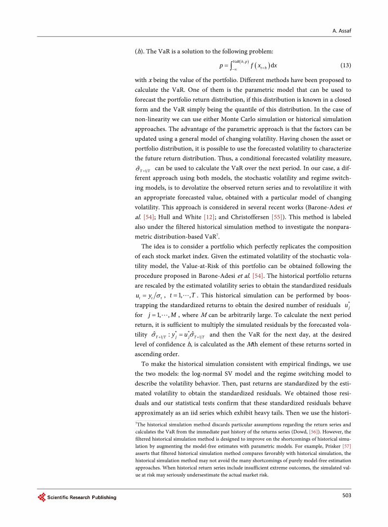
(h). The VaR is a solution to the following problem:
( )( ),d
VaR h pt hp f x x+−∞
= ∫ (13)
with x being the value of the portfolio. Different methods have been proposed to calculate the VaR. One of them is the parametric model that can be used to forecast the portfolio return distribution, if this distribution is known in a closed form and the VaR simply being the quantile of this distribution. In the case of non-linearity we can use either Monte Carlo simulation or historical simulation approaches. The advantage of the parametric approach is that the factors can be updated using a general model of changing volatility. Having chosen the asset or portfolio distribution, it is possible to use the forecasted volatility to characterize the future return distribution. Thus, a conditional forecasted volatility measure,
1ˆT Tσ + can be used to calculate the VaR over the next period. In our case, a dif-ferent approach using both models, the stochastic volatility and regime switch-ing models, is to devolatize the observed return series and to revolatilize it with an appropriate forecasted value, obtained with a particular model of changing volatility. This approach is considered in several recent works (Barone-Adesi et al. [54]; Hull and White [12]; and Christoffersen [55]). This method is labeled also under the filtered historical simulation method to investigate the nonpara-metric distribution-based VaR7.
The idea is to consider a portfolio which perfectly replicates the composition of each stock market index. Given the estimated volatility of the stochastic vola-tility model, the Value-at-Risk of this portfolio can be obtained following the procedure proposed in Barone-Adesi et al. [54]. The historical portfolio returns are rescaled by the estimated volatility series to obtain the standardized residuals
t t tu y σ= , 1, ,t T= . This historical simulation can be performed by boos- trapping the standardized returns to obtain the desired number of residuals *
ju
for 1, ,j M= , where M can be arbitrarily large. To calculate the next period return, it is sufficient to multiply the simulated residuals by the forecasted vola-tility * *
1 1ˆ ˆ:T T j j T Ty uσ σ+ += and then the VaR for the next day, at the desired level of confidence h, is calculated as the Mth element of these returns sorted in ascending order.
To make the historical simulation consistent with empirical findings, we use the two models: the log-normal SV model and the regime switching model to describe the volatility behavior. Then, past returns are standardized by the esti-mated volatility to obtain the standardized residuals. We obtained those resi-duals and our statistical tests confirm that these standardized residuals behave approximately as an iid series which exhibit heavy tails. Then we use the histori-
7The historical simulation method discards particular assumptions regarding the return series and calculates the VaR from the immediate past history of the returns series (Dowd, [56]). However, the filtered historical simulation method is designed to improve on the shortcomings of historical simu-lation by augmenting the model-free estimates with parametric models. For example, Prisker [57] asserts that filtered historical simulation method compares favorably with historical simulation, the historical simulation method may not avoid the many shortcomings of purely model-free estimation approaches. When historical return series include insufficient extreme outcomes, the simulated val-ue at risk may seriously undersestimate the actual market risk.
A. Assaf
504
cal simulation to calculate the Value-at-Risk measures. Finally, to adjust them to the current market conditions, the randomly selected standardized residuals are multiplied by the forecasted volatility obtained from the stochastic volatility and regime switching models.
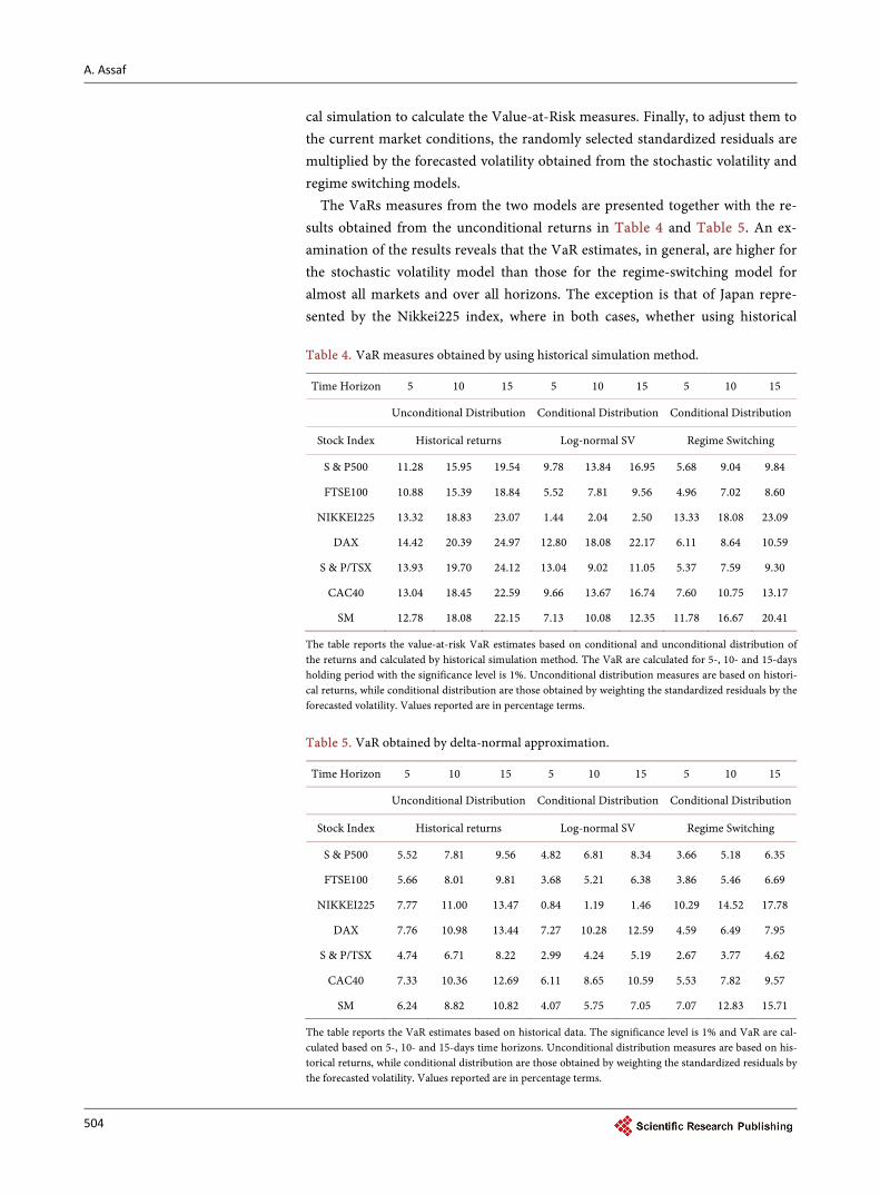
The VaRs measures from the two models are presented together with the re-sults obtained from the unconditional returns in Table 4 and Table 5. An ex-amination of the results reveals that the VaR estimates, in general, are higher for the stochastic volatility model than those for the regime-switching model for almost all markets and over all horizons. The exception is that of Japan repre- sented by the Nikkei225 index, where in both cases, whether using historical Table 4. VaR measures obtained by using historical simulation method.
Time Horizon 5 10 15 5 10 15 5 10 15
Unconditional Distribution Conditional Distribution Conditional Distribution
Stock Index Historical returns Log-normal SV Regime Switching
S & P500 11.28 15.95 19.54 9.78 13.84 16.95 5.68 9.04 9.84
FTSE100 10.88 15.39 18.84 5.52 7.81 9.56 4.96 7.02 8.60
NIKKEI225 13.32 18.83 23.07 1.44 2.04 2.50 13.33 18.08 23.09
DAX 14.42 20.39 24.97 12.80 18.08 22.17 6.11 8.64 10.59
S & P/TSX 13.93 19.70 24.12 13.04 9.02 11.05 5.37 7.59 9.30
CAC40 13.04 18.45 22.59 9.66 13.67 16.74 7.60 10.75 13.17
SM 12.78 18.08 22.15 7.13 10.08 12.35 11.78 16.67 20.41
The table reports the value-at-risk VaR estimates based on conditional and unconditional distribution of the returns and calculated by historical simulation method. The VaR are calculated for 5-, 10- and 15-days holding period with the significance level is 1%. Unconditional distribution measures are based on histori-cal returns, while conditional distribution are those obtained by weighting the standardized residuals by the forecasted volatility. Values reported are in percentage terms.
Table 5. VaR obtained by delta-normal approximation.
Time Horizon 5 10 15 5 10 15 5 10 15
Unconditional Distribution Conditional Distribution Conditional Distribution
Stock Index Historical returns Log-normal SV Regime Switching
S & P500 5.52 7.81 9.56 4.82 6.81 8.34 3.66 5.18 6.35
FTSE100 5.66 8.01 9.81 3.68 5.21 6.38 3.86 5.46 6.69
NIKKEI225 7.77 11.00 13.47 0.84 1.19 1.46 10.29 14.52 17.78
DAX 7.76 10.98 13.44 7.27 10.28 12.59 4.59 6.49 7.95
S & P/TSX 4.74 6.71 8.22 2.99 4.24 5.19 2.67 3.77 4.62
CAC40 7.33 10.36 12.69 6.11 8.65 10.59 5.53 7.82 9.57
SM 6.24 8.82 10.82 4.07 5.75 7.05 7.07 12.83 15.71
The table reports the VaR estimates based on historical data. The significance level is 1% and VaR are cal-culated based on 5-, 10- and 15-days time horizons. Unconditional distribution measures are based on his-torical returns, while conditional distribution are those obtained by weighting the standardized residuals by the forecasted volatility. Values reported are in percentage terms.

A. Assaf
505
simulation or delta-normal approximation, the stochastic volatility model gene-rates lower VaR values than those obtained from the regime switching model. Then comparing the VaRs calculated directly from the two models with those obtained from the unconditional distribution of returns, we find that the two models generate smaller VaRs. When we consider the time horizon and its im-pact on the calculation of the Value-at-Risk measures, we find that VaRs in-crease with the time horizon; generally, and according to the regime switching model, VaRs increase more slowly with horizon than the SV approach.
6. Backtesting the VaR Results
The Value-at-Risk 1p
tVaR + measure promises that the actual return will only be worse than the 1
ptVaR + forecast p * 100 of the time. Given a time series of past
ex-ante VaR forecasts and past ex-post returns, we can define the “hit sequence” of VaR violations as:
, 1 11
, 1 1
1, if0, if
ppf t t
t ppf t t
R VaRI
R VaR+ +
++ +
< −= > (14)
The hit sequence returns a 1 on day t + 1 if the loss on that day was larger than the VaR number predicted in advance for that day. If the VaR was not vi-olated, then the hit sequence returns a 0. When backtesting our models, we con-struct a sequence { }1 1
Tt t
I + + across T days indicating when the past violations occurred. We implement the following three test statistics derived from Christo- ffersen [58]: the unconditional, independence, and conditional coverage8. Chris- toffersen [58] idea is to separate out the particular predictions being tested, and then test each prediction separately. The first of these is that the model generates the “correct” frequency of exceedances, which is in this context is described as the prediction of correct unconditional coverage. The other prediction is that exceedances are independent of each other. This later prediction is important in so far as it suggests that exceedances should not be clustered over time. To ex-plain the Christoffersen [58] approach, we briefly explain the three tests.
6.1. Unconditional Coverage Testing
According to this test, we are interested in testing if the fraction of violations obtained from our models, call it π, is significantly different from the promised fraction, p. We call this the unconditional coverage hypothesis. To test this, we write the likelihood of an i.i.d. Bernoulli (π) hit sequence as:
( ) ( ) ( )1 01 11
11 1t t
TI TI T
tL π π π π π+ +−
=
= − = −∏ (15)
where T0 and T1 are the number of 0s and 1s in the sample. π can be estimated from 1T Tπ = —that is, the observed fraction of violations in the sequence. Plugging the estimate back into the likelihood function gives the optimized like-
8For other methods and elements in backtesting VaR models, see Christoffersen and Diebold [59], Christoffersen and Pelletier [60], McNeil and Frey [61], Diebold, Gunther, and Tsay [62], and Di-ebold, Hahn, and Tsay [63].

A. Assaf
506
lihood as:
( ) ( ) ( )0 11 11 T TL T T T Tπ = − .
Under the unconditional coverage null hypothesis that π = p, where p is the known VaR coverage rate, we have the likelihood:
( ) ( ) ( )1 01 11
11 1t t
TI TI T
tL p p p p p+ +−
=
= − = −∏
The unconditional coverage hypothesis using a likelihood ratio test can be checked as:
( ) ( )ˆ2 lnucLR L p L π= − (16)
Asymptotically, as T goes to infinity, this test will be distributed as a χ2 with one degree of freedom. Substituting in the likelihood functions, we write:
( ) ( ) ( ){ }0 0 111 12 ln 1 1T T TT
uc T T T TLR p p = − − − (17)
which follows a χ2. The VaR model is rejected or accepted either using a specific critical value, or calculating the P-value associated with our test statistic.
6.2. Independence Testing
According to this test, the hit sequence is assumed to be dependent over time and that it can be described as a so-called first-order Markov sequence with transition probability matrix:
01 011
11 11
11
π ππ π
− Π = −
.
These transition probabilities simply mean that conditional on today being a nonviolation (that is, It = 0), then the probability of tomorrow being a violation (that is, It+1 = 1) is π01. The probability of tomorrow being a violation given today is also a violation is: π11 = Pr(It = 1 and It+1 = 1). Accordingly, the two probabili-ties π01 and π11 describe the entire process. The probability of a nonviolation fol-lowing a nonviolation is 1 − π01, and the probability of a nonviolation following a violation is 1 − π11. If we observe a sample of T observations, then the likelihood function of the first-order Markov process can be written as:
( ) ( ) ( )00 1001 1101 01 11 111 1T TT T
tL π π π πΠ = − −
where Tij, i, j = 0, 1 is the number of observations with a j following an i. Taking first derivatives with respect to π01 and π11 and setting these derivatives to zero, we can solve for the maximum likelihood estimates:
( )( )01 01 00 01T T Tπ = + and ( )( )11 11 10 11T T Tπ = + .
Using the fact that the probabilities have to sum to one, we have: π00 = 1 − π01 and π10 = 1 − π11, which can be used to determine the matrix of the estimated transition probabilities.
In the case of the hits being independent over time, then the probability of a violation tomorrow does not depend on today being a violation or not, and we

A. Assaf
507
can write π01 = π11 = π. In this case, we can test the independence hypothesis that π01 = π11 using a likelihood ratio test:
( ) ( )1ˆˆ2 lnindLR L Lπ = − Π (18)
following a 21χ . Where L(π) is the likelihood under the alternative hypothesis
from the LRuc test. Although the LRuc test can reject a model that either overestimates or unde-
restimates the true but unobservable VaR, it cannot examine whether the excep-tions are randomly distributed. In a risk management framework, it is important that VaR exceptions be uncorrelated over time, which prompts independence and conditional coverage tests based on the evaluation of interval forecasts. Christoffersen [58] developed independence and conditional coverage tests that jointly investigates whether the total number of failures is equal to the expected one, and the VaR exceptions are independently distributed. In particular, the advantage of Christoffersen’s procedure is that it can reject a model that gene-rates either too many or too few clustered exceptions. Since accurate VaR esti-mates exhibit the property of correct conditional coverage, the hit sequence se-ries must exhibit both correct unconditional coverage and serial independence.
6.3. Conditional Coverage Testing
Ultimately, we care about simultaneously testing if the VaR violations are inde-pendent and the average number of violations is correct. We can test jointly for independence and correct coverage using the conditional coverage test:
( ) ( )1ˆ2 lnccLR L p L = − Π (19)
again following a 22χ distribution and correspond to testing that π01 = π11 = p.
It can be proved that LRcc = LRuc + LRinp. The Christoffersen approach enables us to test both coverage and independence hypotheses at the same time. Moreover, if the model fails a test of both hypotheses combined, his approach enable us to test each hypothesis separately, and so establish where the model failure arises.
The results for the unconditional and conditional coverage tests are reported in Table 6 and Table 7. Table 6 reports the results based on the stochastic vola-tility model, and Table 7 reports those based on the regime switching model. The symbol * indicates that the test did reject the null hypothesis. We use two significance levels of 5% and 1%. If LRuc is statistically insignificant, it implies that the expected and the actual number of observations falling below the VaR estimates are statistically the same. Further, rejection of the null hypothesis in-dicates that the computed VaR estimates are not sufficiently accurate. According to the LRuc test statistics, and at the 5% significance levels, VaR models based on both the stochastic volatility and regime switching models perform relatively the same for all markets, except for FTSE100, where the LRuc rejects the null hypo-thesis. However, according to the LRind and LRcd, the VaR models based on the two volatility models perform again relatively in a similar fashion. The perfor-mance of both models at the 5% significance level is the worst for the S & P/TSX;

A. Assaf
508
Table 6. Unconditional, conditional and independence coverage tests based on log-normal stochastic volatility model.
Unconditional Independence Conditional
1% (LRuc) 5% (LRuc) 1% (LRind) 5% (LRind) 1% (LRcd) 5% (LRcd)
S & P500 0.081 0.224 4.45* 0.479 4.53 0.704
FTSE100 3.701* 1.371 0.368 0.0001 4.070 1.371
NIKKEI225 1.951 0.003 0.552 0.904 2.503 0.907
DAX 1.064 2.296 0.700 0.776 1.765 3.072
S & P/TSX 0.721* 0.148 12.84* 16.01* 13.56* 16.15*
CAC40 3.071* 0.224 10.51* 0.479 13.59 0.704
SM 1.064 2.043 0.700 0.052 1.765 2.095
The table reports the unconditional, conditional and independence coverage tests based on the Log-Normal Stochastic Volatility model. * indicates rejection of the VaR model.
Table 7. Unconditional, conditional and independence coverage tests based on regime switching model.
Unconditional Independence Conditional
1% (LRuc) 5% (LRuc) 1% (LRind) 5% (LRind) 1% (LRcd) 5% (LRcd)
S & P500 1.479 1.176 0.623 0.566 2.102 1.742
FTSE100 5.171* 2.843* 2.252 0.010 7.424* 2.854
NIKKEI225 1.94 0.021 0.552 2.523 2.497 2.545
DAX 5.97* 2.296 2.102 0.035* 8.08* 2.33
S & P/TSX 2.475 1.581 0.486 5.317* 2.962 6.898*
CAC40 1.064 0.829 0.700 0.074 1.765 0.904
SM 3.071* 0.995 2.746* 2.188 5.818* 3.184
The table reports the unconditional, conditional and independence coverage tests based on the regime switching model. * indicates rejection of the VaR model.
this is because of the rejection of both tests and the failure of both models to provide an accurate prediction of the downside risk at the 5% significance level. Further, the backtesting results indicate that the regime switching model per-forms poorly for the DAX series using the LRind test.
7. Conclusion
This paper proposes two models, namely the log stochastic volatility model and regime switching model for calculating value at risk. The two models were ap-plied for international equity markets and then used to forecast future daily vo-latility. Then based on the forecasted daily volatility, we calculated the Value at Risk in each market. It was observed that the two models generate smaller VaRs than the unconditional distributional method. Then, based on each model, it was found that the Japanese market display lower values of Value at Risk under the stochastic volatility model than under the regime switching model. Considering

A. Assaf
509
how the VaRs increase with time horizon, generally and according to the regime switching model, VaRs increase more slowly with horizon than the stochastic volatility model. Finally, we backtest each model and find that the performance of both models is the worst for the S & P/TSX, while the regime switching model does not perform well for the DAX series in some cases. The results have signif-icant implications for risk management, trading and hedging activities as well as in the pricing of equity derivatives.
References [1] Black, F. (1976) Studies of Stock Price Volatility Changes. Proceedings of the 1976
Meetings of the American Statistical Association, Business and Economical Statis-tics Section, 177-181.
[2] Engle, R., Lilien, D. and Robins, R. (1987) Estimating Time-Varying Risk Premia in the Term Structure. The ARCH-M Model. Econometrica, 55, 391-407. https://doi.org/10.2307/1913242
[3] Andersen, T.G., Bollerslev, T. and Diebold, F.X. (2005) Parametric and Nonpara-metric Volatility Measurement. In: Hansen, L.P. and Aït-Sahalia, Y., Eds., Hand-book of Financial Econometrics, North Holland, Amsterdam, 67-137.
[4] Poon, S.H. and Granger, C.W.J. (2003) Forecasting Volatility in Financial Markets: A Review. Journal of Economic Literature, 41, 478-539. https://doi.org/10.1257/.41.2.478
[5] Bollerslev, T., Chou, R.Y. and Kroner, K. (1992) ARCH Modelling in Finance: A Review of the Theory and Empirical Evidence. Journal of Econometrics, 52, 5-59.
[6] Bera, A.K. and Higgins, M.L. (1993) ARCH Modes: Properties, Estimation and Testing. Journal of Economic Surveys, 7, 305-366. https://doi.org/10.1111/j.1467-6419.1993.tb00170.x
[7] Bollerslev, T., Engle, R.F. and Nelson, D.B. (1994) ARCH Models. In: Engle, R.F. and McFadden, D.L., Eds., Handbook of Econometrics, Vol. 4, Elsevier Science, Amsterdam, 2959-3038.
[8] Taylor, S.J. (1986) Modelling Financial Time Series. Wiley, Chichester.
[9] Ghysels, E., Harvey, A.C. and Renault, E. (1996) Stochastic Volatility. In: Maddala, G.S. and Rao, C.R., Eds., Handbook of Statistics, Vol. 14, Statistical Methods in Finance, North-Holland, Amsterdam, 128-198.
[10] Shephard, N. (1996) Statistical Aspects of ARCH and Stochastic Volatility. In: Cox, D.R., Hinkley, D.V. and Barndorff-Nielsen, O.E., Eds., Time Series Models in Eco-nometrics, Finance and Other Fields, Monographs on Statistics and Applied Proba-bility, Vol. 65, Chapman and Hall, 1-67. https://doi.org/10.1007/978-1-4899-2879-5_1
[11] Broto, C. and Ruiz, E. (2004) Estimation Methods for Stochastic Volatility Models: A Survey. Journal of Economic Surveys, 18, 613-649. https://doi.org/10.1111/j.1467-6419.2004.00232.x
[12] Hull, J. and White, A. (1987) The Pricing of Options on Assets with Stochastic Vo-latilities. The Journal of Finance, 42, 281-300. https://doi.org/10.1111/j.1540-6261.1987.tb02568.x
[13] Campbell, J.Y., Lo, A.W. and Mackinlay, A.C. (1997) The Econometrics of Financial Markets. Princeton Press.
[14] Koopman, S. and Hol Uspensky, E. (2002) The Stochastic Volatility in Mean Model:

A. Assaf
510
Empirical Evidence from International Stock Markets. Journal of Applied Econo-metrics, 17, 667-689. https://doi.org/10.1002/jae.652
[15] Goldfeld, S.M. and Quandt, R.E. (1973) A Markov Model for Switching Regressions. Journal of Econometrics, 1, 3-16.
[16] Hamilton, J.D. (1989) A New Approach of the Economic Analysis of Non-Sta- tionary Time Series and the Business Cycle. Econometrica, 57, 357-384. https://doi.org/10.2307/1912559
[17] LeBaron, B. (1992) Some Relationships between Volatility and Serial Correlations in Stock Market Returns. Journal of Business, 65, 199-219. https://doi.org/10.1086/296565
[18] Timmerman, A. (2000) Moments of Markov Switching Models. Journal of Econo-metrics, 96, 75-111.
[19] Ang, A. and Bekaert, G. (2002) International Asset Allocation with Regime Shifts. Review of Financial Studies, 15, 1137-1187. https://doi.org/10.1093/rfs/15.4.1137
[20] Jorion, P. (1988) On Jump Processes in the Foreign Exchange and Stock Markets. Review of Financial Studies, 1, 427-445. https://doi.org/10.1093/rfs/1.4.427
[21] Akgiray, V. and Booth, G. (1988) Mixed Diffusion-Jump Process Modelling of Ex-change Rate Movements. Review of Economics and Statistics Studies, 70, 631-637. https://doi.org/10.2307/1935826
[22] Bates, D. (1996) Jumps and Stochastic Volatility: Exchange Rate Processes Implicit in Deutsche Mark Options. Review of Financial Studies, 9, 69-107. https://doi.org/10.1093/rfs/9.1.69
[23] Bekaert, G, Erb, C., Harvey, C. and Viskanta, T. (1998) Distributional Characteris-tics of Emerging Market Returns and Asset Allocation. Journal of Portfolio Man-agement, 24, 102-116. https://doi.org/10.3905/jpm.24.2.102
[24] Asgharian, H. and Bengtsson, C. (2006) Jump Spillover in International Equity Markets. Journal of Financial Econometrics, 2, 167-203. https://doi.org/10.1093/jjfinec/nbj005
[25] Ang, A. and Chen, J. (2002) Asymmetric Correlations of Equity Portfolios. Journal of Financial Economics, 63, 443-494.
[26] Longin, F. and Solnik, B. (1995) Is the Correlation in International Equity Returns Constant? Journal of International Money and Finance, 14, 3-26.
[27] Karolyi, A. and Stulz, R. (1996) Why Do Markets Move Together? An Investigation of U.S.-Japan Stock Return Movements. Journal of Finance, 51, 951-986. https://doi.org/10.1111/j.1540-6261.1996.tb02713.x
[28] Chakrabarti, R. and Roll, R. (2000) East Asian and Europe during the 1997 Asian Collapse: A Clinical Study of a Financial Crisis. Working Paper, UCLA.
[29] Chollete, L., de la Pena, V. and Lu, C.-C. (2011) International Diversification: A Copula Approach. Journal of Banking and Finance, 35, 403-417.
[30] Buraschi, A., Porchia, P. and Trojani, F. (2010) Correlation Risk and Optimal Port-folio Choice. Journal of Finance, 65, 393-420. https://doi.org/10.1111/j.1540-6261.2009.01533.x
[31] Kuester, K., Mittnik, S. and Paolella, M. (2006) Value-at-Risk Prediction: A Com-parison of Alternative Strategies. Journal of Financial Econometrics, 1, 53-89.
[32] Engle, R. (1982) Autoregressive Conditional Heteroskedasticity with Estimates of the Variance of U.K. Inflation. Econometrica, 50, 987-1008. https://doi.org/10.2307/1912773
[33] Andersen, T.G., Bollerslev, T., Diebold, F.X. and Labys, P. (2001) The Distribution

A. Assaf
511
of Realized Exchange Rate Volatility. Journal of the American Statistical Associa-tion, 96, 42-55. https://doi.org/10.1198/016214501750332965
[34] Andersen, T.G., Bollerslev, T., Diebold, F.X. and Labys, P. (2003) Modeling and Fo-recasting Realized Volatility. Econometrica, 71, 579-626. https://doi.org/10.1111/1468-0262.00418
[35] Melino, A. and Turnbull, S.M. (1990) Pricing Foreign Currency Options with Sto-chastic Volatility. Journal of Econometrics, 45, 239-265.
[36] Harvey, A.C., Ruiz, E. and Shephard, N. (1994) Multivariate Stochastic Variance Models. Review of Economic Studies, 61, 247-264. https://doi.org/10.2307/2297980
[37] Ruiz, E. (1994) Quasi-Maximum Likelihood Estimation of Stochastic Volatility Models. Journal of Econometrics, 63, 289-306.
[38] Gallant, A.R., Hsieh, D.A. and Tauchen, G.E. (1997) Estimation of Stochastic Vola-tility Models with Diagnostics. Journal of Econometrics, 81, 159-192.
[39] Jacquier, E., Polson, N.G. and Rossi, P.E. (1994) Bayesian Analysis of Stochastic Volatility Models (with Discussion) Journal of Business and Economics Statistics, 12, 371-389.
[40] Kim, S., Shephard, N. and Chib, S. (1998) Stochastic Volatility: Likelihood Inference and Comparison with ARCH Models. Review of Economics Studies, 65, 361-393. https://doi.org/10.1111/1467-937X.00050
[41] Shephard, N. and Pitt, M. (1997) Likelihood Analysis of Non-Gaussian Measure-ment Time Series. Biometrika, 84, 653-667. https://doi.org/10.1093/biomet/84.3.653
[42] Durbin, J. and Koopman, S. (1997) Monte Carlo Maximum Likelihood Estimation for Non-Gaussian State Space Models. Biometrika, 84, 669-684. https://doi.org/10.1093/biomet/84.3.669
[43] Ripley, B. (1987) Stochastic Simulation. Wiley, New York. https://doi.org/10.1002/9780470316726
[44] De Jong, P. and Shephard, N. (1995) The Simulation Smoother for Time Series Models. Biometrika, 82, 339-350. https://doi.org/10.1093/biomet/82.2.339
[45] Doornik, J. (1998) Object-Oriented Matrix Programming Using Ox 2.0. Timberlake Consultants Ltd., London. http://www.nuff.ox.ac.uk/Users/Doornik
[46] Koopman, S., Shephard, N. and Doornik, J. (1999) Statistical Algorithms for Models in State Space Using Ssfpack 2.2. Econometrics Journal, 2, 113-166. http://www.ssfpack.com https://doi.org/10.1111/1368-423X.00023
[47] French, K.R., Schwert, G.W. and Stanbaugh, R.F. (1987) Expected Stock Returns and Volatility. Journal of Financial Economic, 19, 3-29.
[48] Poon, S. and Taylor, S.J. (1992) Stock Returns and Volatility: An Empirical Study of the UK Stock Market. Journal of Banking and Finance, 16, 37-59.
[49] Kim, D. and Kon, S. (1994) Alternative Models for the Conditional Heteroscedas-ticity of Stock Returns. Journal of Business, 67, 563-598. https://doi.org/10.1086/296647
[50] Lamoureux, C.G. and Lastrapes, W.D. (1990) Persistence in Variance, Structural Change and the GARCH Model. Journal of Business and Economic Statistics, 8, 225-243. https://doi.org/10.1080/07350015.1990.10509794
[51] Hamilton, J.D. and Susmel, R. (1994) Autoregressive Conditional Heteroskedastici-ty and Changes in Regime. Journal of Econometrics, 64, 307-333.
[52] Hansen, B. (1992) The Likelihood Ratio Test under Nonstandard Conditions: Test-ing the Markov Switching Model of GNP. Journal of Applied Econometrics, 7, S61-

A. Assaf
512
S82. https://doi.org/10.1002/jae.3950070506
[53] Kobayashi, M. and Shi, X. (2003) Testing for EGARCH against Stochastic Volatility Models. Journal of Time Series Analysis, 26, 135-150. https://doi.org/10.1111/j.1467-9892.2005.00394.x
[54] Barone-Adesi, G., Burgoin, F. and Giannopoulos, K. (1998) Don’t Look Back. Risk, 11, 100-104.
[55] Christoffersen, P. (2003) Elements of Financial Risk Management, Academic Press, San Diego.
[56] Dowd, K. (1998) Beyond Value at Risk: The New Science of Risk Management. Wi-ley, New York.
[57] Prisker, M. (2006) The Hidden Dangers of Historical Simulation. Journal of Bank-ing and Finance, 30, 561-582.
[58] Christoffersen, P. (1998) Evaluating Interval Forecasts. International Economic Re-view, 39, 841-862. https://doi.org/10.2307/2527341
[59] Christoffersen, P. and Diebold, F. (2000) How Relevant Is Volatility Forecasting for Financial Risk Management? Review of Economics and Statistics, 82, 12-22. https://doi.org/10.1162/003465300558597
[60] Christoffersen, P. and Pelletier, D. (2003) Backtesting Portfolio Risk Measures: A Duration-Based Approach, Manuscript, McGill University and CIRANO.
[61] McNeil, A. and Frey, R. (2000) Estimation of Tail-Related Risk Measures for Hete-roskedastic Financial Time Series: An Extreme Value Approach. Journal of Empiri-cal Finance, 7, 271-300.
[62] Diebold, F.X., Gunther, T. and Tsay, A. (1998) Evaluating Density Forecasts, with Applications to Financial Risk Management. International Economic Review, 39, 863-883. https://doi.org/10.2307/2527342
[63] Diebold, F.X., Hahn, J. and Tsay, A. (1999) Multivariate Density Forecasts Evalua-tion and Calibration in Financial Risk Management: High Frequency Returns on Foreign Exchange. Review of Economics and Statistics, 81, 661-673. https://doi.org/10.1162/003465399558526
Submit or recommend next manuscript to SCIRP and we will provide best service for you:
Accepting pre-submission inquiries through Email, Facebook, LinkedIn, Twitter, etc. A wide selection of journals (inclusive of 9 subjects, more than 200 journals) Providing 24-hour high-quality service User-friendly online submission system Fair and swift peer-review system Efficient typesetting and proofreading procedure Display of the result of downloads and visits, as well as the number of cited articles Maximum dissemination of your research work
Submit your manuscript at: http://papersubmission.scirp.org/ Or contact [email protected]

Journal of Mathematical Finance, 2017, 7, 513-517 http://www.scirp.org/journal/jmf
ISSN Online: 2162-2442 ISSN Print: 2162-2434
DOI: 10.4236/jmf.2017.72027 May 31, 2017
Valuation of Derivatives on the Cost Variables of the Shipping Market
Christos E. Kountzakis
Department of Statistics and Actuarial-Financial Mathematics, University of the Aegean, Mytilene, Greece
Abstract In this paper, we present stochastic differential equations related to the cost variables of the shipping market. These SDEs arise under the addition of sto-chastic terms on the deterministic differential equations concerning the same variables. The financial interest arises from the fact that these SDEs may be used for the valuation of derivatives on these variables, such as futures, op-tions, and others. Keywords Transport Costs Per Unit of Cargo Turnover, Deadweight, Optimum Speed
1. Variables Which May Be Taken as Primary in Shipping Markets
It is obvious that ship-owners, design the ships in a way that either minimizes the costs or maximizes the earnings arising from it. The relation between the de-sign of a ship and the costs or the earnings is mentioned in Hughes—in [1], Veenstra and Ludemaz—in [2] and in Stopford—in [3]. In the first reference what is mentioned is that ship-owners consider these costs as constant and they are interested in the evolution of the earnings arising from a ship. In the second reference, the authors examine a relation between the technical characteristics of the ship and the earnings. Finally, in the third reference, cost and revenue va-riables related to a ship are separated, according to the impact of them. From Chen—in [4], we take the following relations:
,tm
SaQ
=
where ta denotes the transport costs per unit of cargo turnover, S denotes the transport costs per year and mQ denotes the cargo turnover per year.
How to cite this paper: Kountzakis, C.E. (2017) Valuation of Derivatives on the Cost Variables of the Shipping Market. Journal of Mathematical Finance, 7, 513-517. https://doi.org/10.4236/jmf.2017.72027 Received: March 14, 2016 Accepted: May 28, 2017 Published: May 31, 2017 Copyright © 2017 by author and Scientific Research Publishing Inc. This work is licensed under the Creative Commons Attribution International License (CC BY 4.0). http://creativecommons.org/licenses/by/4.0/
Open Access

C. E. Kountzakis
514
( )( )
2
1 2
1 23
,22
24
m
ps c
a a DW T LQ
a a DWt t
V M
+ ⋅ ⋅=
++ + +
(1)
where 1 2,a a denote the utilization of ship’s deadweight capacity for inbound and outbound voyages, respectively, mQ denotes the cargo turnover per year, DW denotes the deadweight of the ship, T denotes the service days per year, L denotes indicates the voyage distance, and cM denotes the average cargo han-dling rate at port. Also, 1st denotes the time sailing at a service speed for a round voyage, 2st denotes the time of canal transit for a round voyage, 1pt denotes the time for cargo loading and discharging for a round voyage,
2pt de-notes the turn time for a round voyage, and finally the time 3t denotes the extra time at sea and in port for a round voyage. In Chen—in [4], differentiation with respect to sV gives
d d ,m sl s
m s
Q t VQ t V
=
which implies
1d d dd d .t m s s
t m s
a Q t VS Sa S Q S t V
= − = −
Also, in Chen (2011), differentiation of (1), with respect to DW implies
1d d1 ,pm
m
tQ DWQ t DW
= −
which leads to
1d d d1 .pt
t
ta S DWa S t DW
= − −
2. Financial Models and Derivatives
It is obvious that , , , ,t m sa DW Q S V are stochastic, namely they are subject to change during the service time-period [ ]0,Tτ ∈ , due to a variety of unknown factors. We suppose that each of these variables are subject to change, according to an Itô process across the service-time period:
( ) ( ), 1, ,
,
d, d , d ,s
s ss
Va V V B
Vτ
τ τ ττ
τ τ σ τ= +
( ) ( ) 2d , d , d ,S b S f S BS
ττ τ τ
τ
τ τ τ= +
( ) ( ) 3d , d , d .DW h DW g DW BDW
ττ τ τ
τ
τ τ τ= +
By these stochastic differential equations, we make the above differential models more realistic, since we moreover assume that each of these variables has a value-but subject to a variability, because we may not forecast its exact value at a certain time-moment during the time-period [ ]0,T . Also, [ ]0,Tτ ∈ , and
1 2 3, ,B B Bτ τ τ are usual 1-dimensional independent Brownian motions on ,

C. E. Kountzakis
515
modelling the essential factors of uncertainty. If the models for the processes [ ], , , , 0,sV S DW Tτ τ τ τ ∈ are captured, by the differential form we have above we
take: Proposition 1. The Stochastic Differential Equation for ,sV τ is
( ) ( ) [ ]11, ,
d , d , d , 0, .sl ss s
Q t ta V V B TQ t t
ττ τ τ
τ
τ τ σ τ τ= + ∈
Proposition 2. The Stochastic Differential Equation for ,ta τ is
( ) ( )
( ) ( ) ( ) [ ]
,,
,
T1 21,
d, , d
, , , d ,d , 0, ,
t sls
t
ss t t
a tb S a Va t
tf S V B B Tt
ττ τ
τ
τ τ
τ τ τ
τ σ τ τ
= −
+ − ⋅ ∈
where T denotes transpose matrix. We also consider a banking account, namely an assetwhose evolution is
[ ]0d d , 1, 0, .B r B B Tτ τ τ τ τ= = ∈
Valuation
We consider a European call-option on the transport cost per cargo for a certain ship at the end of the service—time T at a strike—price K. The value of the under-lying ‘‘asset’’—which is the cost is now equal to ,t Ta . The payoff of the call-option is equal to
( ), .t Ta K+
−
We also consider a call-option at the cargo ,m TQ at the end of the ser-vice-time having a strike-price 1K . The payoff of the second option is
( ), 1 .m TQ K+
−
The difference of the two markets is that the market of mQ together with B is complete, while the market of the cost ta together with B is incomplete. Hence, the second call-option may be replicated by the classical spot-market theory, see in Musiela and Rutkowski—[5], 5.1.2: The unique equivalent mar-tingale measure for the discounted cargo-market as a spot market is
( )
( )
( )
( )
2
, ,1
1 1, ,
, ,d 1exp , . .d 2, ,
sl sls s
Ts s
s s
t tr a V r a Vt tB T a st tV V
t t
τ τ τ τ
τ τ
τ τ
σ τ σ τ
− − = − −
Under , the price of [ ]*, ,e , 0,r
m mQ Q Tττ τ τ
− = ∈ is
( )* * *1, , ,d , d ,s
m s mtQ V Q Btτ τ τ τσ τ=
where
( )
( )[ ]
,* 1
1,
,, 0, ,
,
sls
ss
tr a VtB B Tt V
t
τ τ
τ τ
τ
ττ τ
σ τ
−= − ∈
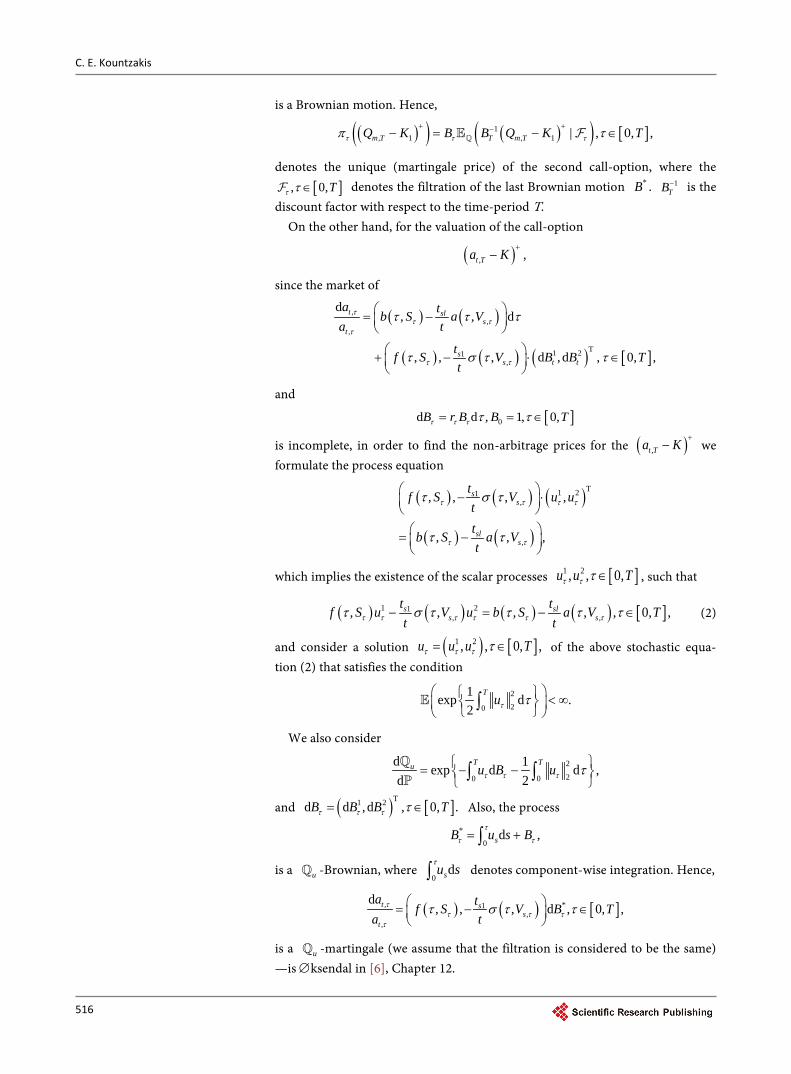
C. E. Kountzakis
516
is a Brownian motion. Hence,
( )( ) ( )( ) [ ]1, 1 , 1 | , 0, ,m T T m TQ K B B Q K Tτ τ τπ τ
+ +−− = − ∈
denotes the unique (martingale price) of the second call-option, where the [ ], 0,Tτ τ ∈ denotes the filtration of the last Brownian motion *B . 1
TB− is the discount factor with respect to the time-period T.
On the other hand, for the valuation of the call-option
( ), ,t Ta K+
−
since the market of
( ) ( )
( ) ( ) ( ) [ ]
,,
,
T1 21,
d, , d
, , , d ,d , 0, ,
t sls
t
ss t t
a tb S a Va t
tf S V B B Tt
ττ τ
τ
τ τ
τ τ τ
τ σ τ τ
= −
+ − ⋅ ∈
and
[ ]0d d , 1, 0,B r B B Tτ τ τ τ τ= = ∈
is incomplete, in order to find the non-arbitrage prices for the ( ),t Ta K+
− we formulate the process equation
( ) ( ) ( )
( ) ( )
T1 21,
,
, , , ,
, , ,
ss
sls
tf S V u uttb S a Vt
τ τ τ τ
τ τ
τ σ τ
τ τ
− ⋅ = −
which implies the existence of the scalar processes [ ]1 2, , 0,u u Tτ τ τ ∈ , such that
( ) ( ) ( ) ( ) [ ]1 21, ,, , , , , 0, ,s sl
s st tf S u V u b S a V Tt tτ τ τ τ τ ττ σ τ τ τ τ− = − ∈ (2)
and consider a solution ( ) [ ]1 2, , 0, ,u u u Tτ τ τ τ= ∈ of the above stochastic equa-tion (2) that satisfies the condition
2
20
1exp d .2
Tuτ τ < ∞
∫
We also consider
2
20 0
d 1exp d d ,d 2
T Tu u B uτ τ τ τ = − − ∫ ∫
and ( ) [ ]T1 2d d ,d , 0, .B B B Tτ τ τ τ= ∈ Also, the process
*0
d ,sB u s Bτ
τ τ= +∫
is a u -Brownian, where 0
dsu sτ
∫ denotes component-wise integration. Hence,
( ) ( ) [ ], *1,
,
d, , , d , 0, ,t s
st
a tf S V B Ta t
ττ τ τ
τ
τ σ τ τ = − ∈
is a u -martingale (we assume that the filtration is considered to be the same) —is ∅ksendal in [6], Chapter 12.

C. E. Kountzakis
517
Uder the above considerations, the following Theorem is obvious: Theorem 3. The non-arbitrage prices of the call-option are—at time period 0:
( )( ) ( )( )( )1 1, ,inf , sup ,
u u uu
T t T T t TB a K B a K+ +− −− −
where 1TB− is the discount factor with respect to the time-period T .
3. Conclusion
The conclusion of this brief paper is that we may discriminate the primary cost variables in the shipping market and the dependence of other variables of this market, by the formulation of Stochastic Differential Equations. These SDE imply the valuation of European options written on the primary variables.
References [1] Hughes, C. (1996) Ship Performance. LLP, London.
[2] Veenstra, A.W. and Ludemaz, M.W. (2006) The Relationship between Design and Economic Performance of Ships. Maritime Policy and Management, 33, 159-171. https://doi.org/10.1080/03088830600612880
[3] Stopford, M. (2009) Maritime Economics. 3rd Edition, Routledge, London. https://doi.org/10.4324/9780203891742
[4] Chen, S. (2011) Modelling and Forecasting in the Dry Bulk Shipping Market. Ph.D. Dissertation, Technical University of Delft, The Netherlands.
[5] Musiela, M. and Rutkowski, M. (1998) Martingale Methods in Financial Modelling. 2nd Edition, Springer.
[6] ∅ksendal, B. (2003) Stochastic Differential Equations—An Introduction with Ap-plications. Springer.
Submit or recommend next manuscript to SCIRP and we will provide best service for you:
Accepting pre-submission inquiries through Email, Facebook, LinkedIn, Twitter, etc. A wide selection of journals (inclusive of 9 subjects, more than 200 journals) Providing 24-hour high-quality service User-friendly online submission system Fair and swift peer-review system Efficient typesetting and proofreading procedure Display of the result of downloads and visits, as well as the number of cited articles Maximum dissemination of your research work
Submit your manuscript at: http://papersubmission.scirp.org/ Or contact [email protected]

9 772162 243007 20