9roxph ,vvxh - sdiwc
TRANSCRIPT

Volume 7, Issue 12017
ISSN 2225-658X (ONLINE)ISSN 2412-6551 (PRINT)

Editor-in-Chief Dr. Rohaya Latip, University Putra Malaysia, Malaysia Editorial Board Abbas M. Al-Ghaili, Universiti Putra Malaysia, Malaysia Ali Sher, American University of Ras Al Khaimah, UAE Altaf Mukati, Bahria University, Pakistan Andre Leon S. Gradvohl, State University of Campinas, Brazil Azizah Abd Manaf, Universiti Teknologi Malaysia, Malaysia Bestoun Ahmed, University Sains Malaysia, Malaysia Carl Latino, Oklahoma State University, USA Dariusz Jacek Jakóbczak, Technical University of Koszalin, Poland Duc T. Pham, University of Bermingham, UK E.George Dharma Prakash Raj, Bharathidasan University, India Elboukhari Mohamed, University Mohamed First, Morocco Eric Atwell, University of Leeds, United Kingdom Eyas El-Qawasmeh, King Saud University, Saudi Arabia Ezendu Ariwa, London Metropolitan University, United Kingdom Fouzi Harrag, UFAS University, Algeria Genge Bela, University of Targu Mures, Romania Guo Bin, Institute Telecom & Management SudParis, France Hadj Hamma Tadjine, Technical university of Clausthal, Germany Hassan Moradi, Qualcomm Inc., USA Isamu Shioya, Hosei University, Japan Jacek Stando, Lodz University of Technology, Poland Jan Platos, VSB-Technical University of Ostrava, Czech Republic Jose Filho, University of Grenoble, France Juan Martinez, Gran Mariscal de Ayacucho University, Venezuela Kaikai Xu, University of Electronic Science and Technology of China, China Khaled A. Mahdi, Kuwait University, Kuwait Ladislav Burita, University of Defence, Czech Republic Maitham Safar, Kuwait University, Kuwait Majid Haghparast, Islamic Azad University, Shahre-Rey Branch, Iran Martin J. Dudziak, Stratford University, USA Mirel Cosulschi, University of Craiova, Romania Mohamed Amine Ferrag, Guelma University, Algeria Monica Vladoiu, PG University of Ploiesti, Romania Nan Zhang, George Washington University, USA Noraziah Ahmad, Universiti Malaysia Pahang, Malaysia Pasquale De Meo, University of Applied Sciences of Porto, Italy Paulino Leite da Silva, ISCAP-IPP University, Portugal Piet Kommers, University of Twente, The Netherlands Radhamani Govindaraju, Damodaran College of Science, India Ramadan Elaiess, University of Benghazi, Libya Rasheed Al-Zharni, King Saud University, Saudi Arabia Su Wu-Chen, Kaohsiung Chang Gung Memorial Hospital, Taiwan Talib Mohammad, University of Botswana, Botswana Tutut Herawan, University Malaysia Pahang, Malaysia Velayutham Pavanasam, Adhiparasakthi Engineering College, India Viacheslav Wolfengagen, JurInfoR-MSU Institute, Russia Wen-Tsai Sung, National Chin-Yi University of Technology, Taiwan Wojciech Zabierowski, Technical University of Lodz, Poland Yasin Kabalci, Nigde University, Turkey Yoshiro Imai, Kagawa University, Japan Zanifa Omary, Dublin Institute of Technology, Ireland Zuqing Zhu, University of Science and Technology of China, China
Publisher The Society of Digital Information and Wireless Communications 20/F, Tower 5, China Hong Kong City, 33 Canton Road, Tsim Sha Tsui, Kowloon, Hong Kong
Further Information Website: http://sdiwc.net/ijdiwc, Email: [email protected], Tel.: (202)-657-4603 - Inside USA; 001(202)-657-4603 - Outside USA.
Overview The SDIWC International Journal of Digital Information and Wireless Communications is a refereed online journal designed to address the networking community from both academia and industry, to discuss recent advances in the broad and quickly-evolving fields of computer and communication networks, technology futures, national policies and standards and to highlight key issues, identify trends, and develop visions for the digital information domain. In the field of Wireless communications; the topics include: Antenna systems and design, Channel Modeling and Propagation, Coding for Wireless Systems, Multiuser and Multiple Access Schemes, Optical Wireless Communications, Resource Allocation over Wireless Networks, Security, Authentication and Cryptography for Wireless Networks, Signal Processing Techniques and Tools, Software and Cognitive Radio, Wireless Traffic and Routing Ad-hoc networks, and Wireless system architectures and applications. As one of the most important aims of this journal is to increase the usage and impact of knowledge as well as increasing the visibility and ease of use of scientific materials, IJDIWC does NOT CHARGE authors for any publication fee for online publishing of their materials in the journal and does NOT CHARGE readers or their institutions for accessing to the published materials.
Permissions International Journal of Digital Information and Wireless Communications (IJDIWC) is an open access journal which means that all content is freely available without charge to the user or his/her institution. Users are allowed to read, download, copy, distribute, print, search, or link to the full texts of the articles in this journal without asking prior permission from the publisher or the author. This is in accordance with the BOAI definition of open access. Disclaimer Statements of fact and opinion in the articles in the International Journal of Digital Information and Wireless Communications (IJDIWC) are those of the respective authors and contributors and not of the International Journal of Digital Information and Wireless Communications (IJDIWC) or The Society of Digital Information and Wireless Communications (SDIWC). Neither The Society of Digital Information and Wireless Communications nor International Journal of Digital Information and Wireless Communications (IJDIWC) make any representation, express or implied, in respect of the accuracy of the material in this journal and cannot accept any legal responsibility or liability as to the errors or omissions that may be made. The reader should make his/her own evaluation as to the appropriateness or otherwise of any experimental technique described. Copyright © 2017 sdiwc.net, All Rights Reserved The issue date is January 2017.
International Journal of DIGITAL INFORMATION AND WIRELESS COMMUNICATIONS

PAPER TITLE AUTHORS PAGES
COMPARATIVE ANALYSES ON LOGO IMAGE DESIGNS BETWEEN ARAB AND JAPAN
Ahmad Eibo, Toshiyuki Yamashita, Keiko Kasamatsu
1
PRIORITY ACCESS MECHANISM FOR IMPROVING RESPONSIVENESS TO USERS THROUGH CACHE SERVER AND PRIORITY ACCESS MANAGEMENT MECHANISM
Hisanori Mizobuchi, Keizo Saisho 10
THE STRESS RELIEF EFFECTS OF WRIST WARMING AFTER MENTAL WORKLOAD
Ayami Ejiri, Keiko Kasamatsu 18
ACCELERATED TRAFfiC MODEL BASED ON PSYCHOLOGICAL EFFECTS Takahiro Suzuki, Shihoko Tanabe, Isamu Shioya
26
FINDING WEAK LINKS IN SUPPLY CHAIN CASE STUDY: THAI FROZEN SHRIMP INDUSTRY
Patchanee Patitad, Hidetsugu Suto, Woramol Chaowarat Watanabe
35
ENERGY EXPENDITURE PER BIT MINIMIZATION INTO MB-OFDM UWB SYSTEMS
Houda Chihi, Reza Zaeem, Ridha Bouallegue
42
A SURVEY OF FOUR ROUTING PROTOCOLS FOR WIRELESS SENSOR NETWORKS
Raid Zaghal, Saeed Salah, Fadi Alyounis
49
TABLE OF CONTENTS Original Articles
IJDIWC Volume 7, Issue No. 1 2017
ISSN 2225-658X (Online) ISSN 2412-6551 (Print)

Comparative Analyses on Logo Image Designs between
Arab and Japan
○Ahmad Eibo, Toshiyuki Yamashita, Keiko Kasamatsu
Tokyo Metropolitan University
6-6 Asahigaoka, Hino. Tokyo 191-0065 Japan
ABSTRACT
With the present announcement of the International
Olympic Committee (IOC) that upcoming 2020
Olympic Games is scheduled to be held in Tokyo and
with various initiatives of Japanese government aimed
at increasing foreign visitors to Tokyo and stimulating
greater foreign products consumption, Arabian products
are beginning to spread throughout Japan reginal
market. This paper is divided into two surveys. Survey I
and survey II compare products and corporate logos of
Arabic alphabetic design to products logos of Japanese
characters design and corporate logos of English
alphabetic design, respectively. Factorial invariances
showed that extracted main images -- “Familiar &
Favorable”, and “Creative & Innovative, “Traditional &
Consistent” -- were the same in both surveys.
Unpredictably our application of cluster analyses for
survey I as well as average scores comparison of survey
II revealed that Arabic logotypes designs are creative
but not as familiar to Japanese people as English
alphabetic logotypes. More importantly rough sets
analyses clarified that logo familiarity image correlates
with the familiarity of language characters used in
design to be known by consumers. Our findings
highlighted future work new theme and suggested that
in order to promote Arabic corporate and products in the
Japanese marketplace, it is extremely important to
familiarize Japanese with the Arabic alphabets.
KEYWORDS
Arab, Japan, 2020 Olympic, Logos, Design, Cluster
analyses, Rough sets.
1 INTRODUCTION
Although people read periodicals for less than ten
minutes per day on average, they watch television
for about three hours per day, and outdoors they see
many billboards and shop fronts. Within this visual
“the clamor of market”, people form impressions
of corporate identities and products brands.
Enhancing a corporation’s image is important for
corporate survival in the current competitive
marketplace. Among the strategies incorporated for
obtaining effective brand image is logo formation,
which represents a vital appeal in commercials for
consumer products. Logos appear on television,
packaging, letterhead, business cards, advertising
signs, annual reports, and product designs. Logos
are considered a critical in-store recognition aid for
speeding up the selection process for preferred
product. This explains why researches on the
psychological effects of logo design structures are
many [1, 2, 3] Okata & Yamashita [4] have
aggregated these previous studies into three effects:
1) Recognition: People’s awareness of logo’s
existence, 2) A common shared meaning:
Commonality between people’s perception of logo
and intended logo’s image, and 3) Positive effect:
Logo design’s favorable impression on people.
Since these three relatively improve consumer
products purchase in marketplace and employment
for human resource professionals, they are
arguably able to influence the logo industry
significantly [4, 10].
2 PROBLEM STATEMENT
With the lack of resources in Japan, the Arab world
with its resource of oil has been important to Japan
great economic development. Although Arab oil
contribution to Japan is historical, it is unfortunate
to declare that Japan’s image in Arab is still
ambivalent in contrast to the Arab world where
people’s image in Japan is being extremely positive
due to the diverse curricula of compulsory
education being taught in most of the Arab
countries. Although this had reflected trade relation
unfavorably between both ends [5] “made in Arab”
products have begun to increase recently in Japan
marketplace, in part, as a result of the development
of diplomatic and commercial communications
between Japan and Arab countries [6]. However,
International Journal of Digital Information and Wireless Communications (IJDIWC) 7(1): 1-9The Society of Digital Information and Wireless Communications, 2017 ISSN: 2225-658X (Online); ISSN 2412-6551 (Print)
1

since Japan has adopted English in compulsory
education even daily life Japanese people have
become much more knowledgeable of English
language alphabets than other foreign languages
[7]. The need for appropriate image of Arabic
alphabetic logotype design to influence Japanese
people positively is compelling.
3 PURPOSE
Although evolutionary psychology suggests that
people from different cultures response to visual
stimuli is genetically programmed and relatively
immune from cultural influence [8] a number of
empirical research data indicates that emotional
reaction to individual’s preferred design attributes
is influenced by cultural differences [9, 10]
Therefore, in order to understanding how logos
bring image or cause impression on people, it is
extremely important to grasp the psychological
effect of logo’s attributes on one’s personality traits.
It was the mismatched image and diversity rhetoric
of Arab in Japanese society that led us to examine
the differences of Japanese consumer perception
towards the influence of Arabic, Japanese, and
English logotypes images attempting to utilize our
findings in improving Arabic logotypes design for
the Japan marketplace.
4 SURVEY I
In survey I, in order to ensure that the questions are
designed to address the needs of this research and
are asking the correct questions, the questionnaire
structure was based on empirical Japanese research previously conducted [4, 11, 12] A booklet of 12
pages where each contained pair of product Logos
from Arab and Japan. Each pair of logos appeared
on separate page with five-point rating scales: (“1.
Yes”, “2. Somewhat Yes”, “3. Neither way”, “4.
Somewhat No”, and “5. No”) to be evaluated by
respondents. Subjects participated in this study
were 22 undergraduate students (18 females and 4
males). We firstly show all participants four
example logos (Biscuits, Soft drink, Soap, Fruit
can) to illustrate the task, and then gave them the
questionnaire booklets to simultaneously rate
his/her answers one at a time, each logo of the
following 12 products: Washing detergent,
Laundry Detergent, Glass detergent, Dishwasher
detergent, Soft drink, Perfume, Soap, Beer,
Biscuits, Fruit can, Toilet Paper, and Tobacco in
local Japan and Arab market as shown in Figure 1.
Figure 1. Example of product logos
The description of the 12 logo image questions are
as follows: “1. Energetic: motion sense”, “2.
Innovative: inspiration sense, “3. Familiar:
recognition sense”, “4. Consistent: solid sense”, “5.
Reliable: professionalism sense”, “6. Favorable:
goodness sense”, “7. Traditional: custom sense”,
“8. Promotable: progress sense”, “9. Futuristic:
vision sense”, “10. Creative: skill sense”, “11.
Characteristic: feature sense”, and “12. Luxurious:
class sense.”
4.1 Factor Analyses
The validity of cross-individual comparison scores
are vital to many practices in applied psychological
research. The premise of researching in individual
personality traits or perception is to construct
comparability; hence the utilization of an adequate
analyses method is important for true
representation of the collected data. Relative
factorial invariance is widely tested with Factor
Analysis that allows one to empirically test
obtained data and then translate it into factor
analytic language, so that the main factors can be
clarified [4, 10] In our survey, the correlation
matrix in the evaluation data of the 22 products
logotypes was examined by Factor Analysis
method application [10] Analytic procedures
International Journal of Digital Information and Wireless Communications (IJDIWC) 7(1): 1-9The Society of Digital Information and Wireless Communications, 2017 ISSN: 2225-658X (Online); ISSN 2412-6551 (Print)
2
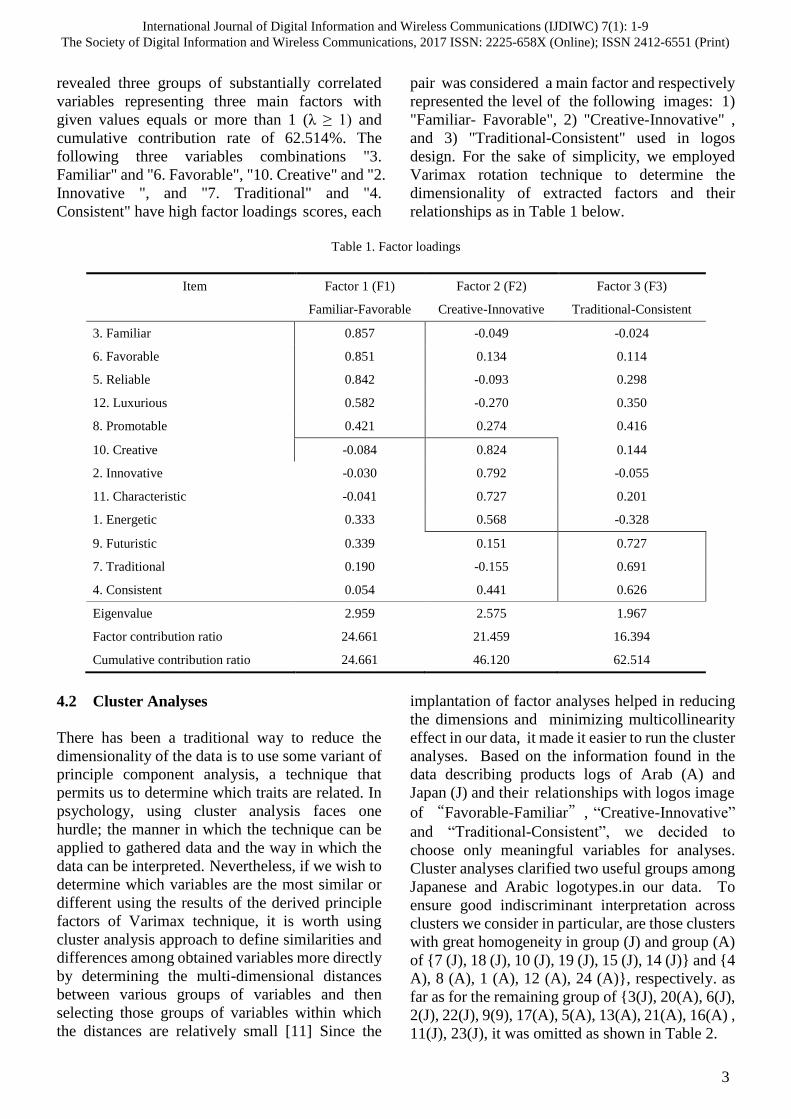
revealed three groups of substantially correlated
variables representing three main factors with
given values equals or more than 1 (λ ≥ 1) and
cumulative contribution rate of 62.514%. The
following three variables combinations "3.
Familiar" and "6. Favorable", "10. Creative" and "2.
Innovative ", and "7. Traditional" and "4.
Consistent" have high factor loadings scores, each
pair was considered a main factor and respectively
represented the level of the following images: 1)
"Familiar- Favorable", 2) "Creative-Innovative" ,
and 3) "Traditional-Consistent" used in logos
design. For the sake of simplicity, we employed
Varimax rotation technique to determine the
dimensionality of extracted factors and their
relationships as in Table 1 below.
Table 1. Factor loadings
Item Factor 1 (F1) Factor 2 (F2) Factor 3 (F3)
Familiar-Favorable Creative-Innovative Traditional-Consistent
3. Familiar 0.857 -0.049 -0.024
6. Favorable 0.851 0.134 0.114
5. Reliable 0.842 -0.093 0.298
12. Luxurious 0.582 -0.270 0.350
8. Promotable 0.421 0.274 0.416
10. Creative -0.084 0.824 0.144
2. Innovative -0.030 0.792 -0.055
11. Characteristic -0.041 0.727 0.201
1. Energetic 0.333 0.568 -0.328
9. Futuristic 0.339 0.151 0.727
7. Traditional 0.190 -0.155 0.691
4. Consistent 0.054 0.441 0.626
Eigenvalue 2.959 2.575 1.967
Factor contribution ratio 24.661 21.459 16.394
Cumulative contribution ratio 24.661 46.120 62.514
4.2 Cluster Analyses
There has been a traditional way to reduce the
dimensionality of the data is to use some variant of
principle component analysis, a technique that
permits us to determine which traits are related. In
psychology, using cluster analysis faces one
hurdle; the manner in which the technique can be
applied to gathered data and the way in which the
data can be interpreted. Nevertheless, if we wish to
determine which variables are the most similar or
different using the results of the derived principle
factors of Varimax technique, it is worth using
cluster analysis approach to define similarities and
differences among obtained variables more directly
by determining the multi-dimensional distances
between various groups of variables and then
selecting those groups of variables within which
the distances are relatively small [11] Since the
implantation of factor analyses helped in reducing the dimensions and minimizing multicollinearity
effect in our data, it made it easier to run the cluster
analyses. Based on the information found in the
data describing products logs of Arab (A) and
Japan (J) and their relationships with logos image
of “Favorable-Familiar”, “Creative-Innovative”
and “Traditional-Consistent”, we decided to
choose only meaningful variables for analyses.
Cluster analyses clarified two useful groups among
Japanese and Arabic logotypes.in our data. To
ensure good indiscriminant interpretation across
clusters we consider in particular, are those clusters
with great homogeneity in group (J) and group (A)
of {7 (J), 18 (J), 10 (J), 19 (J), 15 (J), 14 (J)} and {4
A), 8 (A), 1 (A), 12 (A), 24 (A)}, respectively. as
far as for the remaining group of {3(J), 20(A), 6(J),
2(J), 22(J), 9(9), 17(A), 5(A), 13(A), 21(A), 16(A) ,
11(J), 23(J), it was omitted as shown in Table 2.
International Journal of Digital Information and Wireless Communications (IJDIWC) 7(1): 1-9The Society of Digital Information and Wireless Communications, 2017 ISSN: 2225-658X (Online); ISSN 2412-6551 (Print)
3
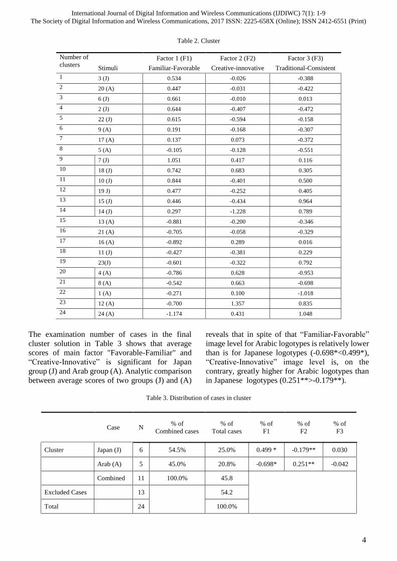
Table 2. Cluster
The examination number of cases in the final
cluster solution in Table 3 shows that average
scores of main factor "Favorable-Familiar" and
“Creative-Innovative” is significant for Japan
group (J) and Arab group (A). Analytic comparison
between average scores of two groups (J) and (A)
reveals that in spite of that “Familiar-Favorable”
image level for Arabic logotypes is relatively lower
than is for Japanese logotypes (-0.698*<0.499*),
“Creative-Innovative” image level is, on the
contrary, greatly higher for Arabic logotypes than
in Japanese logotypes (0.251**>-0.179**).
Table 3. Distribution of cases in cluster
Number of
clusters Factor 1 (F1) Factor 2 (F2) Factor 3 (F3)
Stimuli Familiar-Favorable Creative-innovative Traditional-Consistent
1 3 (J) 0.534 -0.026 -0.388
2 20 (A) 0.447 -0.031 -0.422
3 6 (J) 0.661 -0.010 0.013
4 2 (J) 0.644 -0.407 -0.472
5 22 (J) 0.615 -0.594 -0.158
6 9 (A) 0.191 -0.168 -0.307
7 17 (A) 0.137 0.073 -0.372
8 5 (A) -0.105 -0.128 -0.551
9 7 (J) 1.051 0.417 0.116
10 18 (J) 0.742 0.683 0.305
11 10 (J) 0.844 -0.401 0.500
12 19 J) 0.477 -0.252 0.405
13 15 (J) 0.446 -0.434 0.964
14 14 (J) 0.297 -1.228 0.789
15 13 (A) -0.881 -0.200 -0.346
16 21 (A) -0.705 -0.058 -0.329
17 16 (A) -0.892 0.289 0.016
18 11 (J) -0.427 -0.381 0.229
19 23(J) -0.601 -0.322 0.792
20 4 (A) -0.786 0.628 -0.953
21 8 (A) -0.542 0.663 -0.698
22 1 (A) -0.271 0.100 -1.018
23 12 (A) -0.700 1.357 0.835
24 24 (A) -1.174 0.431 1.048
Case N % of
Combined cases
% of
Total cases
% of
F1
% of
F2
% of
F3
Cluster Japan (J) 6 54.5% 25.0% 0.499 * -0.179** 0.030
Arab (A) 5 45.0% 20.8% -0.698* 0.251** -0.042
Combined 11 100.0% 45.8
Excluded Cases 13
54.2
Total 24 100.0%
International Journal of Digital Information and Wireless Communications (IJDIWC) 7(1): 1-9The Society of Digital Information and Wireless Communications, 2017 ISSN: 2225-658X (Online); ISSN 2412-6551 (Print)
4

4.3 Result & Discussion
The results of clusters analyses were consistent
with prior works [12] this is especially true for
"Familiar-Favorable", "Creative-Innovative and
"Traditional-Consistent" main images, where the
patterns of the path estimates are consistent across
response variables and obtained clusters. But the
effect of unfamiliarity & creativity on participants
was higher for Arabic logotypes than for Japanese
logotypes. Our findings reveal that the perception
of Arabic and Japanese logotypes by Japanese
people towards the same kind of product differs
because of the unfamiliarity with Arabic language
alphabets and familiarity with the Japanese
characters, however, a strong image of creativity
was found in Arabic logo design attributes
although Arabic alphabets are not well-known in
Japan. Would our finding be the same for English
logos design? In other words, the question of
whether or not English alphabetic logotypes would
have about the same effect of Arab logos design on
Japanese people is worth asking. A study done by
Takahashi [13] showed that although Japanese
graduate students do not often understand English,
they do not have negative image of it. The
sociocultural situation in Japanese is truly unique due to American culture influence. The possible
reasons for the extensive filtering of American
culture into the Japan are manifold. In Japan,
generally Western languages were seen as
symbolic of progress and modernization. After
World War II Japanese aspired to creating a
country similar in economic and technological
progression to the United States of America.
Through desire to emulate the American way of
life, the Japanese people began, willingly, to adopt
much more American culture [14] In recent
decades, even though Japan has certainly reached
its goal of becoming a modern, economically
powerful society, America still maintain its allure
to the Japanese as a culture which is fashionable,
and generally appealing. This is not simply a matter
of cultural contact, but part of a complex process of
identity reformation mediated by a sense of
tendency related to the representation and
appropriation of the “other”. Despite the evident
importance of research on such a wide-ranging and
complex phenomenon of cultural and differences,
hardly any attempt has been made until recently,
hence in this paper we wanted to include studying
the significance of English logotype influence [15]
5 SURVEY II
Because we found that Arabic logotypes are
unfamiliar by Japanese people, we can now test
whether or not this result is the same for English
logotypes. Since the first survey examined Arabic
and Japanese logotypes, our interest in the second
one was focused on Arabic and English logotypes.
50 undergraduate students (35 males and 15
females) participated in this survey. We applied the
same questionnaire structure used in survey I for 20
well-known logos of 10 global corporate in Arab
and Japan with Arabic and English alphabetic
logotypes respectively: FedEx, Burger King, CNN,
Subway, Tide, Baskin Robbin, Vodafone,
Starbucks, Coca Cola, and Adidas as is shown in
Figure 4.
Figure 2. Examples of corporate logos
5. 1 Factor Analyses
In survey II, factor analyses also prioritize three
significant factors resembling main factors in
survey I “3. Familiar” and “6. Favorable”, “10.
Creative” and “2. Innovative”, and “7. Traditional”
and “4. Consistent” as is shown in Table 4.
Astonishingly, the three influential images of
corporate and products logotypes are the same in
both surveys as it has been found in relevant
research conducted previously [11, 16] In Table 4.
Since the result is relatively consistent with what
International Journal of Digital Information and Wireless Communications (IJDIWC) 7(1): 1-9The Society of Digital Information and Wireless Communications, 2017 ISSN: 2225-658X (Online); ISSN 2412-6551 (Print)
5

survey I concluded, it fairly suggest that the
association made between three logo images of
“Familiar-Favorable”, “Creative-Innovative”, and
“Traditional-Consistent” is highly significant.
Thus, the combination of logo structures are being
designed based on specific set between the three
seems to influence Japanese people perception, and
therefore it is recommended to be considered as
main images in logos design for products and
corporate.
Table 4. Factor loadings
the average Scores of factor 1 (F1) and factor 2
(F2) in Figure 3 shows that the image of
“Familiar-Favorable” scored low for Arabic
logotypes and high for English logotypes although
logo designed marks are similar in shapes and
colors relatively, indicating presence of unfamiliar
attribute towards Arabic logotypes.
Figure 3. Factor 2 and Factor 3Average scores
In the contrast to what we found in Figure 3, the
average Scores of factor 2 (F2) and factor 4 (F3) in
Figure 4 reveals that the image of
“Innovative-Creative” scored high in Arabic
logotypes than in English logotypes. It clarifies
high level of creative attribute towards Arabic
logotypes.
Figure 4. Factor 2 and Factor 3Average scores
Item Factor 1 (F1) Factor 2 (F2) Factor 3 (F3)
Traditional-Consistent Familiar-Favorable Creative-Innovative
4. Consistent 0.79 0.19 -0.08
7. Traditional 0.75 0.11 0.15
9. Futuristic 0.71 0.35 0.23
12. Luxurious 0.67 -0.01 0.43
5. Reliable 0.67 0.55 0.05
8. Promotable 0.53 0.41 0.38
6. Favorable 0.39 0.75 0.17
1. Energetic -0.08 0.75 0.37
3. Familiar 0.36 0.75 0.09
11. Characteristic 0.08 0.12 0.83
10. Creative 0.16 0.20 0.78
2. Innovative 0.12 0.44 0.62
Eigenvalue 3.20 2.56 2.28
Factor contribution ratio 26.64 21.34 18.97
Cumulative contribution ratio 26.64 47.98 66.94
International Journal of Digital Information and Wireless Communications (IJDIWC) 7(1): 1-9The Society of Digital Information and Wireless Communications, 2017 ISSN: 2225-658X (Online); ISSN 2412-6551 (Print)
6

5.2 Rough Sets Analyses
Although Factor Analyses extracted three
dimensions of the main corporate logo images
"Tradition-Consistent", "Favorable-Familiar", and
“Creative-Innovative,” how logo attributes
influence consumer perception was still unclear. In
order to obtain adequate contraction of minimum
attributes combination as well as identifying the
psychological relationship between logo samples
and consumer perception, an additional
mathematical analyses approach known as Rough
Sets proposed by Zdzisław Pawlak [17] would be
imperative. In psychology, it is been used widely
for data explicit interpretation and accurate
minimal sets by revealing the causal relationship
between “If” and “Then” rule decisions [16, 18, 19,
20] Rough Set analyses require binary variables
for a case or an event. Each variable takes the
values 0 or 1, that is, each case or event is
conceived as a configuration of conditions. Data have the form of a decision table in which the
columns represent causal variables (logical
variables) may take the value 0 or 1and the rows
represent cases [21] In Table 5 the composition
decision table below between logo design structure
(logo mark, logo entirety, and logotype) and main
logo three images (Traditional-Consistent,
Familiar-Favorable, and Innovative-Creative) is
shown in Table 5: 1) Target set U, 2) Attribute Set
Condition C, and 3) Attribute Set Decision D.
Target set U is made of corporate logo, Attribute
Set Condition C consists of the following
equations: C = {Logo Mark (1 for Present, 0 for
Absent), Active-Inactive (1 for Active, 0 for
inactive), Solid sense (1 for Present, 0 for Absent),
Logotype thickness (1 for thin, 0 for thick),
Logotype Italic sense (1 for Present, 0 for Absent),
Logotype variation of base line (1 for Present, 0 for
Absent), Logotype white color processing of (1 for
Present, 0 for Absent), Logotype language type (1
for Known, 0 for Unknown}, and finally Attribute
Set Decision D of three main images of corporate
logo D = {Traditional-Consistent and
Familiar-Favorable, and Creative-Innovative} with
1 given value when image score is greater than zero
and 2 value when image score is lower than zero.
At this stage of data preparations, the number of
attribute decision sets can be minimized by logical
contraction.
Table 5. Decision Table
Target
Set U
Attribute Set Condition C Attribute Set Decision D
Logo
Mark Logo Entirety Logo Type (Font)
Traditional
Consistent
Familiar
Favorable
Innovative
Creative
Sample Present Absent
Active Inactive
Solid Sense
Thickness Italic Sense
Baseline Change
White Color
Processing
Language
J1 0 0 1 0 0 0 0 1 1 1 2
A1 0 0 0 0 0 0 0 0 2 2 1
J2 1 1 0 0 1 0 0 1 2 1 2
A2 1 1 0 0 1 0 0 0 2 2 1
J3 0 0 0 0 0 0 1 1 2 1 2
A3 0 0 1 0 0 0 1 0 2 2 2
J4 0 1 0 0 1 0 1 1 2 1 1
A4 0 1 1 0 0 0 1 0 2 2 2
J5 1 0 0 0 1 0 0 1 2 1 1
A5 1 0 1 0 1 0 1 0 2 1 1
J6 0 0 0 0 0 0 0 1 2 1 2
A6 0 0 1 0 1 0 0 0 2 2 2
J7 1 0 0 0 0 0 0 1 1 1 1
A7 1 1 1 0 0 0 1 0 2 2 2
J8 1 0 1
1 2 1
A8 1 0 1
1 2 1
J9 1 1 1 1 1 0 1 1 1 1 1
A9 0 1 1 1 1 0 1 0 2 2 1
J10 1 0 1 0 0 0 0 1 1 1 1
A10 1 0 1 1 0 0 1 0 1 2 2
International Journal of Digital Information and Wireless Communications (IJDIWC) 7(1): 1-9The Society of Digital Information and Wireless Communications, 2017 ISSN: 2225-658X (Online); ISSN 2412-6551 (Print)
7

The goal of rough ret analyses is to specify the
different configurations of the causal variables that
produce the outcome variable. And the goal of
logical minimization is to represent the data in a
rationally constructed shorthand manner as the
Table 6 below demonstrates [22,23] The sets
shown in this table were minimized by contraction
technique for interpretation by the following
complementary rules were applied based on
decision class weights (0.9), (0.6), and (0.444)
respectively : 1) If [known language] exists in
corporate logo Then ["Familiar- Favorable" Image]
exists, 2) If [Solid sense present] And [known
language] exist in corporate logo Then
[“Traditional-Consistent” Image] exists, and 3) If
[Logo Entirety Active]
And [Italic Sense Present] And [White Color
Processing Present] exist in corporate logo Then
[“Creative-innovative” Image] exists. Extracted
sets indicated that in order to impart the image of
"Familiar- Favorable" in logo design it is important
that the language character used in logo attributes
to be known by the consumer. Moreover, the
image of “Creative-Innovative” correlates directly
with [Logo Entirety] and [Logotype], and not
necessarily with [Logo Mark], it reveals that
"Creative-Innovative" image in logo design can be
imparted by the combination of logo attributes used
in logo design not by concentrate on a specific
attribute such as active sense in Coca Cola or
thickness sense in FedEx logo.
Table 6. Contraction
Decision
Class
C
Logo Mark Logo Entirety Logotype (Font)
Present-Absent Active-Inactive Solid Sense Thickness Italic Sense Baseline
Change
White Color
Processing Language
Present Absent Active Inactive Present Absent Thin Thick Present Absent Present Absent Present Absent Known Un-
known
Traditional
Consistent
2
0.6
0.6
0.6
0.6
0.6
0.6
0.6
0.6
0.6 0.6
Familiar
Favorable 1
0.9
Innovative
Creative
3
0.444
0.444
0.444
0.444
0.444
0.444
6 CONCLUSION & FUTURE WORK
Inspection of the factor loadings in both surveys
prioritized three influential images significantly
and substantially different from zero value
“Familiar-Favorable”, “Creative-Innovative”, and
“Traditional-Consistent”. This clarifies that logo
design characteristics are captured by the same
factorial structures and also strongly outperforms
simultaneous basics for Arabic logotypes design
industry in commercial sectors with three
dimensions: 1) Familiarity, 2) Creativity, and 3)
Traditionalism. Respectively, the analyses of
clusters as well as average scores comparison in
survey I and Survey II confirmed that English
alphabetic logotypes are familiar to Japanese
people than Arabic alphabetic logotypes most
likely due to the influence of American culture.
Also since rough sets analyses linked between
familiarity in logo image with the familiarity of
language used in logo design to be recognized by
Japanese, it suggests that the familiarization of
Arabic language to Japan consumers is important
to promotion Arab corporate and products in Japan
marketplace. But in spite of the unfamiliarity in
Arabic language, Arabic alphabetic logotypes seem
to impart a strong image of creativity for Japanese
people, perhaps because of hidden similarity
between Arabic alphabets and Japanese characters.
Future research can extend our findings in several
meaningful ways for upcoming 2020 Olympic.
Most notably a cross-cultural research between
Arab and Japan investigating Arabic and Japanese
language calligraphy psychological influence on
one’s personality traits.
International Journal of Digital Information and Wireless Communications (IJDIWC) 7(1): 1-9The Society of Digital Information and Wireless Communications, 2017 ISSN: 2225-658X (Online); ISSN 2412-6551 (Print)
8

REFERENCES
1. Janiszewski, C., & Meyvis, T., “Effects of rand logo
complexity, repetition, and spacing on processing
fluency and judgment”, Journal of Consumer Research,
28(1), pp.18-32(2001)
2. Stafford, M.R., Tripp, C., & Bienstock, C.C., “The
influence of advertising logo characteristics on audience
perception of a nonprofit theatrical organization”,
Journal of Current Issues and Research in Advertising,
26(1), pp.37-45(2004)
3. Melewar, T.C., Hussey, G., & Srivoravilai,
N.,“Corporate visual identity: The re-branding of France
Telecom”, Journal of Brand Management, 12(5),
pp.379-394 (2005)
4. Okata, Y., Yamashita, T., “an exploratory study of
corporate logo image”, Tokai University Fukuoka Junior
College Bulletin, 9, pp.1-7 (2007)
5. Hosaka, S., “A Historical Perspective of Pre-Oil
Relations”, Kyoto Bulletin of Islamic Area Studies,
4-1&2, 4-1&2 (March 2011), pp.3–24
6. Tatsuki, D., “English Language Education in Japan:
Transitions and Challenges”, Journal of Foreign Studies,
pp. 31-42. (2011)
7. Okai, H., & Ishikawa, K., “A Case Study in Gifu City,
Japan: Perceptions and Attitude toward Islam and
Muslims”, Waseda University, Institute of Multi-ethnic
and Multi-generational Societies, Determinants of Local
Residents, Bulletin, 10, PP1-20 (2010)
8. Adams, R. B., Jr., H. L. Gordon, A. A. Baird, N. Ambady,
R. E. Kleck., “ Effects of gaze on amygdala sensitivity to
anger and fear faces”, Science 300 (5625) 1536 (2003)
9. Perfetti, C., Y. Liu, L. H. Tan., “The lexical constituency
model: Some implications of research on Chinese for
general theories of reading”, Psych. Rev. 112(1) 43–59
(2005)
10. Zhang, Y., L. Feick, L. J. Price., “The impact of
self-construal on aesthetic preference for angular versus
rounded Shapes”, Personality Soc. Psych. Bull. 32(6)
794–805 (2006)
11. Yamashita, T., Paku, R. T. Yoshi., “Comparative Study
of Japanese and Korean corporate logo image”, Japan
modern studies, 29 pp.371- 387 (2010)
12. Johnson, S. C., Hierarchical Clustering Schemes,
Psychometrika 32 pp. 241-255 (1967)
13. Henderson, P. W., J. A. Cote, S. M. Leong, B. Schmitt,
Building strong brands in Asia: Selecting the visual
components of image to maximize brand strength,
Internat. J. Res. Marketing 20(4) pp.297–313 (2003)
14. Takashi, K., “A sociolinguistic analysis of English
borrowings in Japanese advertising texts”, World
Englishes, 9(3) pp. 327-341 (1990)
15. MacGregor, L., “The Language of shop signs in Tokyo”,
English Today”, 19(1) pp. 18-23 (2003)
16. Yamashita, T., Toshiaki, K., “Rough sets analysis on
corporate logo and corporate image”, Tokyo humanities
report Metropolitan University, No.485 (Psychology 55),
pp.53-67 (2014)
17. Pawlak, Z., “Rough sets”, International Journal of
Information and Computer Sciences, 11(5), pp.341
-356(1982)
18. Skowron, A., J. Komorowski, Z. Pawlak, L.Polkowski.,
“A rough set perspective on data and knowledge, in: W.
Kloesgen, J. Zytkow (eds.)”, Handbook of KDD, Oxford
University Press, 134-149 (2002)
19. Polkowski, L., A. Skowron., “Rough mereological
calculi granules: a rough set approach to computation,
computational intelligence”, An International Journal 17,
472-479 (2001)
20. Polkowski, L., “Rough Sets: Mathematical Foundations,
Advances in Soft Computing, Physica – Verlag”, A
Springer-Verlag Company (2002)
21. Ragin, C.C., “The comparative method: Moving beyond
qualitative and quantitative strategies”, Berkeley
University of California Press (1987)
22. Mori N., Tanaka H., and Inoue, B., “Rough sets and
sensibility: reasoning and knowledge acquisition from
data”, Kaibundo Publisher (2004)
23. Pawlak, Z., “Rough sets: Theoretical Aspects of
Reasoning about Data”, Dordrecht: Kluwer Academic
Publishers (1991)
International Journal of Digital Information and Wireless Communications (IJDIWC) 7(1): 1-9The Society of Digital Information and Wireless Communications, 2017 ISSN: 2225-658X (Online); ISSN 2412-6551 (Print)
9

Priority Access Mechanism for Improving Responsiveness to Users through
Cache Server and Priority Access Management Mechanism
Hisanori MIZOBUCHI and Keizo SAISHO
Kagawa University
2217-20 Hayashi-cho, Takamatsu 761-0396, Japan
[email protected], [email protected]
ABSTRACT
This research aims at caching non-interactive
dynamic contents such as news and weather, and
blogs for read only users. We think that there is no
problem for users even if they browse these dynamic
contents in several seconds later. However, practical
use of cached dynamic contents requires quick cache
update. We have developed Priority Access
Mechanism and Priority Access Management
Mechanism. Priority Access Mechanism assigns the
quota of the computer resource to handle access from
cache servers independently of other accesses. By
this mechanism, Web server can respond to cache
servers quickly even if there is huge amount of other
requests. Priority Access Management Mechanism
registers new cache server and client from which
accesses to be recognized as priority access. By
registering client, users can update their page using
Web interface without stress. This paper describes
design, implementation and evaluation of Priority
Access Mechanism, and Priority Access Management
Mechanism. Through experiments, we confirm that it
is possible to adjust the quota of the computer
resources to process accesses from cache server,
cache server can update contents in a short time and
respond to users quickly, and cache server and client
can be registered dynamically.
KEYWORDS
priority access, cache server, quick response,
dynamic contents, dynamic registration 1 INTRODUCTION
Recently the Internet becomes widely used and a
lot of people use it. Surge of traffic caused by
certain events such as a topic of TV show and
disaster increases load of servers and delays
response from them. Load distribution technics
are generally used to avoid overload of servers.
There is a Web system that uses cache servers or
mirror servers for load distribution. In this paper,
we call such Web system “distributed Web
system”. We developed a distributed Web
system consisting of Web server and cache
servers. The system varies the number of cache
servers according to the load[1]. We think that dynamic contents such as news
and weather, and blogs for read only users can
be cached in short term by setting the expiration
date of cache of dynamic contents very short. It
can be lighten server load sufficiently with short
term caching. However, it cannot use this idea
when cache update takes long time. In order to
avoid this situation, we divide accesses into two
groups, one is priority access group including
accesses from cache servers and the other is
normal access group including accesses from
clients. And then we develop Priority Access
Mechanism to process priority access group
prior to normal access group. Since the
mechanism can serve dynamic contents to cache
servers quickly, the quality of cache contents
served by cache servers can be improved. Priority Access Mechanism regards accesses
from specific (priority) hosts as priority accesses.
By registering cache servers as priority hosts,
accesses from cache servers are processed prior
to other accesses. Since cache servers are
appended or removed according to load
dynamically, we also develop Priority Access
Management Mechanism which registers
appended cache server as priority host to Priority
Access Mechanism and deletes registration of
removed cache server. By registering client as
priority host, users can update their page using
Web interface without stress even when Web
server stays in overload. In this paper, design, implementation and
evaluation of Priority Access Mechanism and
Priority Access Management Mechanism are
described.
International Journal of Digital Information and Wireless Communications (IJDIWC) 7(1): 10-17The Society of Digital Information and Wireless Communications, 2017 ISSN: 2225-658X (Online); ISSN 2412-6551 (Print)
10

2 RELATED WORK
There are several researches to classify accesses
into some classes and assign them appropriate
priority. Lu, L., Cherkasova, L., de Nitto Personè, V., Mi,
N., and Smirni, E. presented “a novel autonomic
session based admission control policy”[2]. It
uses queue to control the number of active
simultaneous processing accesses and the
number of maximum acceptance accesses, and
reject accesses over maximum acceptance
number. It is similar to our system but ours’ does
not reject the access belonging to priority access
group and processes it prior to other accesses. Holton, D.R.W., Younas, M., and Awan, I.U.
developed and evaluated the system that was
assumed to be used in e-commerce area[3]. They
contended that “the requests received from a
Web portal should generally get higher priority
as such requests are more likely to lead to
purchases”. Received access is stored in the
queue corresponding to type of it. If priority of
incoming access is higher than that of current
processed access then it is suspended and
incoming access is processed. Elnikety, S., Nahum, E., Tracey, J., and
Zwaenepoel, W. determined the priority of a
process according to the size of job[4]. By
lowering the priority of a big job, it raises the
overall responsiveness. Cherkasova, L. and
Phaal, P. introduced a session based admission
control to ensure that longer sessions can be
completed[5]. If a server is functioning near its
capacity, a new session will be rejected. These
researches emphasize to prevent overloading and
maintain total throughput at peak rather than to
ensure the response time of each classes.
Menaséc, D.A., Fonseca, R., Almeida, V.A.F.,
and Mendes, M.A. present a family of priority-
based resource management policies for e-
commerce servers[6]. This aims at optimizing
revenue/sec instead of focusing on conventional
performance metrics. Their target is
improvement of responsiveness to clients and
single Web server is assumed. In our research,
responsiveness is improved by using multiple
cache servers, and the quality of resource served
by them is raised by priority processing.
3 DESIGN AND IMPLEMENTATION OF PRIORITY ACCESS MECHANISM
Figure 1 shows Priority Access Mechanism we
developed. It is implemented based on NAP-
Web[7] developed in our laboratory. Before describing Priority Access Mechanism,
we describe NAP-Web. It is the access control
mechanism developed as a module of Apache[8].
When response of access is expected to take too
long time caused by overload, NAP-Web returns
a ticket to notify the next access time to the
client which sends the access. When the client
re-accesses at the notified time, NAP-Web
accepts the access as far as possible. In order to control accesses, NAP-Web uses
Run_Ready (RR), Wait queue (WA) and
Re_Access queue (RA) and Next_Wait table.
They are shown in left part of Figure 1. RR
stores currently processing accesses. Thus the
size of RR decides the maximum processing
number of accesses. By limiting the size of RR,
Web server load can be suppressed. WA stores
accesses waiting for processing by FIFO manner.
Next_Wait keeps ticket information to identify
access whether it is re-accessed or not. RA stores
re-accesses by FIFO manner. When RR is not
full, the incoming access is entered in RR. When
RR is full and all accesses in WA and RA are
expected to finish within upper limit time, it is
queued in WA. In our experiments the upper
limit time is set 4 seconds. Otherwise, the ticket
is created, recorded on Next_Wait and returned
the client which sends the access. Thus NAP-
Web does not pile up accesses waiting for TCP
connection, and new connection request can be
established immediately. If re-access reaches at
the notified time, it is queued in RA. When RR
goes to not full, the head of WA goes to RR if
Figure 1. Priority access mechanism based on NAP-Web
International Journal of Digital Information and Wireless Communications (IJDIWC) 7(1): 10-17The Society of Digital Information and Wireless Communications, 2017 ISSN: 2225-658X (Online); ISSN 2412-6551 (Print)
11

PRR
1 2
RR 10 (1,10) (2,10)
20 (1,20) (2,20)
WA is not empty, and the head of RA goes to
WA if RA is not empty. We now describe Priority Access Mechanism
shown in right part of Figure 1. Accesses are
classified into two groups. One is priority access
group handled by Priority Access Mechanism.
The other is normal access group handled by
original NAP-Web. After this we call original
NAP-Web “Normal Access Mechanism”.
Pri_Run_Ready (PRR) stores currently
processing priority accesses. Pri_Wait queue
(PWA) stores priority accesses waiting for
processing. By limiting the number of
simultaneous priority accesses under the size of
PWA, priority accesses are always processing or
waiting with keeping TCP connection. Normal
Access Mechanism and Priority Access
Mechanism are placed in parallel. The number of
current processing accesses is sum of the number
of accesses in RR and PRR. We divert queues of NAP-Web except
Next_Wait and RA to Priority Access
Mechanism and add selector. By changing the
maximum number of access in RR and PRR,
system can control computer resources for
processing priority access. In our system, source
IP address is used to identify priority access.
Selector checks source IP address of reached
access. If it is one of one of IP addresses of
cache servers, the selector passes the access to
Priority Access Mechanism. Otherwise, it passes
the access to Normal Access Mechanism. In
experiments in Section 4, IP addresses of priority
client and cache server are hard coded. 4 EVALUATION OF PRIORITY ACCESS
MECHANISM In this section, influence of priority access on
response time of normal access, adjustment of
the quota of the computer resource to priority
access and the effect on response time to clients
through cache server are examined. 4.1 Influence of Priority Access on Response
Time of Normal Access and Adjustment of the Quota of the Computer Resource to Priority Access
Priority Access Mechanism is examined whether
it could adjust the quota of computer resource to
process priority access by changing the ratio of
the size of RR and PRR. The throughputs of both
groups were measured with several combination
of the size of RR and PRR.
4.1.1 Experiment Description
Experiment environment is shown in Figure 2.
Each client issues the designated simultaneous
accesses severally to a bulletin board system
(ASKA BBS [9]) on origin server. Each client
generates designated number of threads. Each
thread accesses repeatedly to origin server
simultaneously. The upper limit of the response
time of the NAP-Web is set to 4 seconds. The
combination of size of RR and PRR used in the
experiments is shown in Table 1. (n, m) shows
(the size of PRR, the size of RR). The total
number of threads on normal clients is 3,000
which is enough number to make origin server
stay in overload. The number of threads on
priority client is 5 which is enough number to fill
PRR. Normal clients start access at the
beginning of experiments and priority client
starts access at after 200 seconds later. The
reason to delay starting time of priority client is
that re-access time prediction is disordered just
after starting normal access.
Figure 2. Experiment environment for throughput
examination
Table 1. Combination of RR and PRR
International Journal of Digital Information and Wireless Communications (IJDIWC) 7(1): 10-17The Society of Digital Information and Wireless Communications, 2017 ISSN: 2225-658X (Online); ISSN 2412-6551 (Print)
12

(0, 20) (1, 10) (1, 20)
(2, 10) (2, 20)
40
(s) 30
Time 20
Response 10
0
100 200 300 400 500 600 700 800
Time (s)
Thro
ugh
pu
t
4.1.2 Results of Experiments
Figure 3 shows the response time of normal
access. Moving average of response time which
window size is 10 seconds is used to plot graphs.
Graphs are separated into 2 groups in all
parameters. This is because there are 2 kinds of
accesses. One succeeds at the first time access,
and the other requires re-access. Response time
required re-access is sum of the processing time
in the first access, the waiting time and the
processing time in the re-access. The lower
group includes accesses that succeed at the first
200
150
100
50
0
(1, 10) (1, 20) (2, 10) (2, 20)
100 200 300 400 500 600 700 800
Time (s)
time, and the upper group includes accesses that
succeed by re-access. Response time in lower
group is about 4 seconds which is almost equal
to upper limit stay in WA and RA. This shows
that maximum staying time in WA and RA is not
so influenced by priority access. Response time
without priority access (0, 20) in upper group is
about 20 seconds in all time. However response
time after starting priority access (200 seconds
point) in upper group lengthens and is disordered.
The response time with high percentage of PRR
is longer than that of low percentage of PRR. Priority access throughput (THp), normal access
throughput (THn) and total throughput (THt) are
shown in Figure 4. They are placed lower, center
and upper location, respectively. THt is sum of
THp and THn. THt is about 160 in all
combinations even if the sizes of the RR and
PRR are changed. It shows that THt is not
influenced by the size of them. Table 2 shows
the percentage of PRR in sum of PRR and RR
and average percentage of THp in THt for 600
seconds (between 200 to 800 seconds). We
expected that the percentage of THp was roughly
Figure 3. Response time of normal access
Figure 4. THp, THn and THt
Table 2. The Percentage of Throughput
Percentage of PRR
in sum of PRR and
RR
Average percentage of
THp in THt
(1, 10) 9.1 21.4
(1, 20) 4.8 22.0
(2, 10) 16.7 31.3
(2, 20) 9.1 27.8
equal to the percentage of PRR. The percentage
of THp is, however, higher 12.3% to 18.7% than
that of PRR. Moreover the percentage of THp
with (1, 10) is different from that of THp with
(2, 20). On the other hand, the percentage of
THp with (2, 20) is higher than that of THp with
(1, 20), and the percentage of THp with (2, 10) is
also higher than that of THp with (1, 10).
Magnitude relation between percentage of THp
and percentage of PRR with same size of RR is
preserved. This result shows that it is possible to
adjust the quota of computer resource to process
priority access but it is insufficient. Improvement
of adjustment precision is future work. 4.2 The Effect on Response Time to Clients
Through Cache Server The purpose of this experiment is to confirm that
Priority Access Mechanism can reduce response
time to clients through cache server. As shown in
Figure 5, we use origin server with our
mechanism, cache server, direct clients accessing
origin server, and indirect client accessing cache
server. While origin server is overloaded by
numerical simultaneous accesses from direct
clients, indirect client accesses to cache server.
The expiration date of cache is set a few seconds
for caching dynamic contents. The response time
to direct and indirect clients is measured.
International Journal of Digital Information and Wireless Communications (IJDIWC) 7(1): 10-17The Society of Digital Information and Wireless Communications, 2017 ISSN: 2225-658X (Online); ISSN 2412-6551 (Print)
13

Figure 5. A schematic of the experimental society
4.2.1 Experiment Description Cache server is configured as a reverse proxy of
origin server. To add the reverse proxy function
and the caching function to the cache server. We
use “mod_proxy” and “mod_disk_cache”
modules of Apache, respectively. All clients
access ASKA BBS with read only mode to serve
same contents to both clients. The expiration
date of cache is set to 5 seconds. We think it is
short enough to cache BBS type contents. The
total number of threads on direct clients is 2,000
which is enough number to make origin server
stay in overload. The number of threads on
indirect client is 300 with which cache server
does not stay in overload. 4.2.2 Experimental Result
Figure 6 shows response time on indirect client.
Graphs are separated into 2 groups because of
existing two kinds of response. The lower group
includes response time to return cached content
directly. The upper group includes response time
with cache update. The average cache update
time is about 0.25 seconds. We think that this
time enables update at several seconds interval
and dynamic read only contents can be cached. Figure 7 shows response time on direct client.
Graphs are separated into 2 groups and response
time of both groups is longer than 4 seconds like
Figure 3. This is because that direct access is
controlled by Normal Access Mechanism.
Response time to direct access is too longer than
that of indirect access.
Figure 6. Response time on indirect client with
Priority Access Mechanism
Figure 7. Response time on direct client with
Priority Access Mechanism
Next, we experiment using origin server without
Priority Access Mechanism. Original NAP-Web
should be used but cache server does not support
re-access. Thus we use original Apache for the
experiment. Figure 8 shows response time on
indirect client. Similar to Figure 6, response time
is separated into 2 groups, but response time
with cache update is about 7 seconds which is
about 25 times longer than response time with
cache update using Priority Access Mechanism.
Figure 9 shows response time on direct clients.
Figure 8. Response time on indirect client without
Priority Access Mechanism
International Journal of Digital Information and Wireless Communications (IJDIWC) 7(1): 10-17The Society of Digital Information and Wireless Communications, 2017 ISSN: 2225-658X (Online); ISSN 2412-6551 (Print)
14

Figure 9. Response time on direct client without
Priority Access Mechanism
Range of response time is about 5 to 10 seconds.
This range is same as range of response time on
indirect client with cache update. It is thinkable
that the response time to indirect client with
update is similar to graphs in Figure 7 when
original NAP-Web used. These results show the effectiveness Priority
Access Mechanism. 5 DEVELOPMENT OF PRIORITY
ACCESS MANAGEMENT MECHANISM As mentioned at the end of Section 3,
experiments in Section 4 are achieved using hard
coded IP addresses to recognize priority accesses.
In order to append and remove cache servers
provided on cloud environment dynamically, we
develop Priority Access Management
Mechanism which registers appended cache
server to Priority Access Mechanism as priority
host and deletes registration information of
remove cache server. By registering clients that
owner are administrator and user who want to
update his page using Web interface, they can
get fast response. In the following subsections, target recognition
method, design and function evaluation of
Dynamic Registration Method are described. 5.1 Consideration of Target Recognition
Method IP address and cookie can be used to recognize
whether an access is priority access or not. In our
implementation of Priority Access Mechanism
used in Section 4, IP addresses of priority client
and cache server are stored in IP address array
(IP-Array) statically, and source IP address of
arrival access is checked whether it is included
in IP-Array or not. It is easy to implement the
method using IP address by appending a function
which registers IP address of appended priority
host with IP-Array and deletes IP address of
removed priority host from IP-Array. If a client that does not have global IP address
and access Web server using NAT, and
registered as a priority client, accesses from
other clients that share global IP address with
registered clients are also recognized as priority
access. In such case, the method using IP address
cannot be used. This problem can be solved by
using cookie. In order to handle cookie, we
introduce priority key array (PC-Array) and scan
function of PC-Array into Priority Access
Mechanism. However, this method requires that
each host needs to correspond to cookie.
Therefore, it may not be able to be used
depending on the cache server. Since cache servers always have global IP
address in our distributed Web system, we
decide that the method using IP address is used
for cache server and the method using cookie is
used for clients. Registration and delete of IP
address of cache server are done by cache server
management system. Registration and delete of
cookie are done by users having their page on
Web server. 5.2 Design
Priority Access Management Mechanism has an
Authentication CGI, an API for registering and
deleting priority IP address and cookie, and a
status page for showing the registration list.
Status page is used for managing. Authentication CGI is the interface of Priority
Access Management Mechanism, and used for
registers cookie. It examines whether user who
want to register his host is legal or not, and then
requests priority key to API and returns priority
cookie including priority key as shown in Figure
10. Priority key has an expiration date, and it is
deleted automatically if there is no access for a
certain period of time. API has interfaces that generate, register and
return priority key, and register and delete
International Journal of Digital Information and Wireless Communications (IJDIWC) 7(1): 10-17The Society of Digital Information and Wireless Communications, 2017 ISSN: 2225-658X (Online); ISSN 2412-6551 (Print)
15

1. Request
priority cookie
Priority Access Management Mechanism
2. Request Priority key
5.3 Function Evaluation Functions of the implemented mechanism are
4. Return
Priority Cookie
Authen-
tication
CGI
3. Return
Priority key
Registering and
deleting
API
examined. We create status page which shows
the number of accesses in each queue. By
accessing the status page as the destination page, 5. Access with
Priority Cookie
Desti-
nation
page
1. Examine whether the
current registered number
of priority hosts is exceeds
the upper-limit.
This trial succeeds if it is not
exceeds
2. Generate random string.
3. Register as priority key.
4. Return priority key.
we can confirm the access is processed by which
mechanism; Normal Assess Mechanism or
Priority Access Mechanism.
Figure 11 shows the result of cookie version. No
client is registered at staring experiment. Figure
11-(a) shows the status page accessed before Figure 10. Registration flow of priority client using cookie
priority IP address. When API is required to
register or delete priority IP address, it checks
where the request come from using source IP
address of it. If the source IP address is same as
the IP address of cache server management
system, it registers or deletes priority IP address.
API also deletes priority key at its expiration
date. Status page shows list of IP addresses in IP-
Array and priority keys in PC-Array, and the
number of accesses in each queue. Now, we present Registration flow of priority
client using cookie shown in Figure 10. 1. A user who wants to get priority cookie
accesses Authentication CGI.
2. Authentication CGI examines whether he is
legal user or not. If he pass the examination,
Authentication CGI request API to generate,
register, and return priority key.
3. API examines whether the number of priority
hosts is exceeds the upper-limit or not. If the
number exceeds the upper-limit, the request
fails and returns error information. Otherwise,
the trial succeeds and API generates, registers
and returns priority key.
4. Authentication CGI creates priority cookie
that includes returned priority key and returns
it with redirect information to destination
page.
5. The user can access destination page prior to
normal accesses.
We implement Priority Access Management
Mechanism except deleting function.
registration. Strings at left side denote queue
name and figures at right side denote the number
of accesses included in corresponding queue.
The access is processed by Priority Access
Mechanism because Run_Ready includes one
access and pre_Run_Ready includes no access.
Figure 11-(b) shows the status page accessed
after registration. the access is processed by
Normal Access Mechanism because Run_Ready
includes no access and pre_Run_Ready includes
one access. These results show that a client can
get priority cookie from Priority Access
Management Mechanism and access from the
client is processed by Priority Access
Mechanism. We also experiment using IP address version.
The same results as the experiment using cookie
version is obtained before and after registration
of IP address. There results indicate that Priority Access
Management Mechanism works fine.
(a) Access before registration (b) Access after registration
Figure 11. Queue information
6 CONCLUSION
We have developed Priority Access Mechanism
for access from cache server and Priority Access
Management Mechanism for registering priority
hosts dynamically. We confirm that cache can be
International Journal of Digital Information and Wireless Communications (IJDIWC) 7(1): 10-17The Society of Digital Information and Wireless Communications, 2017 ISSN: 2225-658X (Online); ISSN 2412-6551 (Print)
16

renewed in a short time by Priority Access
Mechanism and then short term cache for
dynamic contents could be possible. And the
mechanism can adjust the quota of the computer
resource to handle access from cache server.
However adjustment precision is insufficient.
We also confirm that Priority Access
Management Mechanism can register priority
hosts dynamically and accesses issued from
registered hosts are processed by Priority Access
Mechanism.
The feature work is as follows.
• Improvement of adjustment precision.
• Evaluation using more realistic situation, e.g., fluctuating the number of accesses over time.
• Evaluation of effectiveness of caching dynamic contents.
• Implementation of deleting function of Priority Access Management Mechanism.
• Integration of Priority Access Mechanism with our distributed Web system.
REFERENCES
1. Horiuchi, A., and Saisho, K., Development of Scaling
Mechanism for Distributed Web System, Proceedings
of 16th IEEE/ACIS International Conference on
Software Engineering, Artificial Intelligence,
Networking and Parallel/Distributed Computing
(SNPD 2015), pp.283-288, 2015.
2. Lu, L., Cherkasova, L., de Nitto Personè, V., Mi, N.,
and Smirni, E., AWAIT: Efficient Overload
Management for Busy Multi-tier Web Services under
Bursty Workloads, Proceedings of the 10th
International Conference on Web Engineering
(ICWE'2010), pp.81-97, 2010.
3. Holton, D.R.W., Younas, M., and Awan, I.U., Priority
scheduling of requests to web portals, Journal of
Systems and Software, Vol.84, Issue 8, 1373-1378,
2011.
4. Elnikety, S., Nahum, E., Tracey, J., and Zwaenepoel,
W., A Method for Transparent Admission Aontrol and
Request Scheduling in E-Commerce Web Sites,
Proceedings of the 13th international conference on
World Wide Web, pp.276-286, 2004.
5. Cherkasova, L. and Phaal, P., Session Based
Admission Control: A Mechanism for Improving the
Performance of an Overloaded Web Server, HPL-98-
119, HP Labs Technical Reports, 1998.
6. Menaséc, D.A., Fonseca, R., Almeida, V.A.F., and
Mendes, M.A., Resource Management Policies For E-
commerce Servers, ACM SIGMETRICS Performance
Evaluation Review, Vol.27, Issue 4, pp.27-35, 2000.
7. Kaji, T. and Saisho, K., Proposal of Web System
“NAP-Web” to Promise Next Access, Proceedings of
International Conference on Instrumentation, Control
and Information Technology (SICE Annual
Conference 2007), pp.959-964, 2007.
8. https://httpd.apache.org/
9. http://www.kent-Web.com/bbs/aska.html
International Journal of Digital Information and Wireless Communications (IJDIWC) 7(1): 10-17The Society of Digital Information and Wireless Communications, 2017 ISSN: 2225-658X (Online); ISSN 2412-6551 (Print)
17

The Stress Relief Effects of Wrist Warming After Mental Workload
Ayami Ejiri and Keiko Kasamatsu
Graduate School of System Design, Tokyo Metropolitan University,
6-6 Asahigaoka, Hino, Tokyo 191-0065, Japan
[email protected], [email protected]
ABSTRACT
To clarify the mental stress relief effects of wrist
warming, we conducted an experiment involving 8
healthy participants and evaluated the differences in
psychological and physiological responses between
using a warm armrest and normal temperature
armrest after mental workload from a timed typing
test.
Psychological responses were evaluated with a
questionnaire: using 21 questionnaire items with 7
mood state categories: “Active”, “Anger”,
“Comfort”, “Relaxed”, “Strained”, “Anxiety /
Uneasiness”, and “Languor/Boredom”. Furthermore,
physiological responses were evaluated with changes
in the 3 following parameters: heart rate, skin
temperature of the base of the little finger, and
galvanic skin temperature. In this experiment, we
used NeXus-10 MARKII for measurement and
BioTrace+ for analysis.
From our findings, when participants used the warm
armrest after mental workload, their questionnaire
scores of “Anxiety /Uneasiness” and “Comfort” were
improved. In addition, we found that, in many of the
participants, the skin temperature of the base of little
finger was increased, although it was not in contact
with the armrest. These results seem to suggest that
wrist warming relieves mental stress.
KEYWORDS
Mental workload, Mental stress relief, Psychological
responses, Heart rate, Skin temperature, Galvanic
Skin Response, Wrist warming, Time pressure.
1 INTRODUCTION
Work methods have been drastically changed by
recent developments in ICT (Information and
Communication Technology).
Currently, office workers commonly use diverse
technologies; devices such as the desktop PC,
Notebook PC, tablet, and smartphone are
extensively employed during work hours for
emailing, writing documents, and programming,
among other activities. These devices are also
used outside work for internet surfing, instant
messaging, net shopping, and playing games.
ICT provides many opportunities for obtaining
necessary information and communication,
without the restrictions to time and location.
However, it imposes increased mental and
physical stress since device displays are looked
at for long periods of time.
In Japan, the Ministry of Health, Labour and
Welfare set out “Guidelines for Industrial Health
Controls of VDT (Visual Display Terminals)
Operations” in 2002 [1].
To reduce office workers’ physical and mental
workloads, this guideline recommends shortened
continuous VDT operation time per day and
constant breaks.
Nevertheless, many workers do not take
voluntary breaks and this increases their health
risk because of prolonged mental and physical
stress.
Many methods have been reported to relieve
mental stress and office workers may select
suitable methods depending on their situation or
condition. Popular methods include exercise,
breathing, aromatherapy, healing music, and
light therapy. However, the effect of tactile
methods and in particular, thermal stimulus has
not been well clarified.
Office workers find it difficult to reduce stress
during working hours. For example, in case of
exercise, a convenient place must be selected,
and for methods such as healing music and
aromatherapy, the influence of and effect on the
surrounding environment must be considered.
Therefore, although many workers are aware of
various stress relief methods, these methods are
usually infeasible in the workplace.
Consequently, we proposed that the use of
thermal stimulus might be an effective method
that can be utilized regularly without the
International Journal of Digital Information and Wireless Communications (IJDIWC) 7(1): 18-25The Society of Digital Information and Wireless Communications, 2017 ISSN: 2225-658X (Online); ISSN 2412-6551 (Print)
18

surrounding environment constituting any
impediment to its use.
Incidentally, in the field of nursing science, a
popular treatment method using thermal
stimulus, called the hot compress, is used for
pain care and relaxation. Researchers have
investigated the effect of the hot compress, using
psychological and physiological parameters [2],
[3]. However, many office workers find it
difficult to employ this technique because they
are not familiar with its use.
Therefore, in this study, we focused on the
mental stress relief effects of thermal stimulus
application to the wrists, a method that may be
easily employed during work hours. In this
study, we aimed to clarify the mental stress relief
effect of wrist warming after mental workload.
2 METHODS
2.1 Experiment Outline
We conducted an experiment to clarify the effect
of wrist warming with 8 healthy participants.
Figure 1 shows the experiment environment and
Table 1 shows the experiment outline.
Figure 1. Experiment Environment
Table 1. Experiment outline
Period March, 2016 - June, 2016
Place Tokyo Metropolitan University
Sensibility Evaluation Laboratory
Participants 8 healthy participants
[age, 20s and 30s]
*male: 6, female: 2
Temperature 22 – 25 degrees Celsius
Number of
tests
Two tests using armrests at different
temperatures
+ trial test for each participant
Mental
workload
Timed typing tasks
All tasks consisted of about 750
Japanese characters with 46% of the
Kanji characters included.
Wrist
warming
method
Armrest with gel pad
1st time: normal temperature gel pad
2nd time: warmed by microwave
* 52 -54 degrees Celsius
Typing
system
Excel form with checking function
Psychological
responses
21 questionnaire items,
with 7 mood s categories
Physiological
responses
Heart rate, skin temperature, and
galvanic skin response.
(detected by NeXus-10 MARKII)
2.2 Experimental Procedure
At first, we have explained the experiment
contents to each participant. Thereafter, they
performed the typing test without any time limit
until they became accustomed to the task. After
this, we conducted the main experiment twice,
on separate days. Throughout the experiments,
participants were seated in a chair.
2.2.1 Trial Typing Test
The typing test was performed untimed until the
participants become used to the task. The
number of characters used were one-third that of
the main experiment. The typing system was the
same as that in the main experiment.
International Journal of Digital Information and Wireless Communications (IJDIWC) 7(1): 18-25The Society of Digital Information and Wireless Communications, 2017 ISSN: 2225-658X (Online); ISSN 2412-6551 (Print)
19

2.2.2 First Experiment
All participants were tested as follows:
Start: Sensors were placed on the
participant
Step 1: The participants kept calm for 5 min
at the start. Their eyes were allowed to be
open.
Step 2: The questionnaire was filled.
Step 3: Complete typing tasks within a set
time.
After the participants read the input paper,
they started typing on the system.
They were required to complete 2 typing
tasks within 50 min. We informed the
participants of the time at 25 min, 40
min, and 45 min, during the tasks.
The experiment was considered
completed if they completed tasks
before 50 min or if the 50 min elapsed.
The latter case was treated as “Time
out”.
Step 4: The questionnaire was filled.
Step 5: The participants kept calm for 7 min
as the rest condition.
The first 2 min was performed as Step 1.
In the next 5 min, the armrest with
normal temperature was used.
Step 6: The questionnaire was filled.
End: The sensors were removed from the
participant.
Notice: The questionnaire used for Step 2, Step 4,
and Step 6 was the same.
We continued to detect with using Nexus-10
MARKII during the experiment. The details of
these are shown in Section 2.7 (Physiological
Responses).
Figure 2 shows the timeline of the experiment.
Figure 2. Timeline of the Experiment
2.2.3 Second Experiment
The participants were tested in the same way as
in the first experiment, except for Step 5.
Step 5:
The first 2 min was the same as Step 1.
For the next 5 min, the warm armrest was
used.
2.3 Mental Workload
We selected the typing test as the mental
workload under VDT operations and utilized
Japanese newspaper articles for selecting nearly
equal numbers of Japanese and Kanji characters.
Furthermore, in order to increase the mental
workload, two requirements were needed for the
typing test to be regarded as completed:
All characters were inputted correctly.
Typing was completed within the set time.
2.4 Wrist Warming Method
We selected the gel pad for the wrist warming
method, which can be warmed by a microwave
and keep warm for a period of time. Although it
loses heat several hours later, it can warmed up
repeatedly.
We used the armrest that comprised the gel pad
wrapped in a towel.
Step 3: Two typing tasks
(Time limit 50 min)
Step 5:
Keep calm (2 min),
Keep calm with armrest (5 min)
Experiment
Times
End
Start
Step 6:
Fill the questionnaire
Step 4:
Fill the questionnaire
Step 2:
Fill the questionnaire
Step 1:
Keep calm (5 min)
International Journal of Digital Information and Wireless Communications (IJDIWC) 7(1): 18-25The Society of Digital Information and Wireless Communications, 2017 ISSN: 2225-658X (Online); ISSN 2412-6551 (Print)
20

2.5 Typing System
We developed the typing form with checking
function via Excel VBA programming.
Figure 3 shows the typing process.
Figure 3. The typing process
(a) Start to type the characters in the input paper
into the Excel form in the desktop PC.
(b) Click the [Check] button on the bottom-right
in the Excel form after all characters are
input.
(c) The typing form confirms whether all
characters are inputted correctly by
comparing with the correct output saved
beforehand.
(d) If all characters are inputted correctly, a
message showing that the task is completed
is displayed on the bottom-left.
(e) When a wrong character is entered, the form
deletes below the sentences including wrong
characters, and a message prompting the
participant to re-type the characters is
displayed on the bottom-left.
(f) The participant re-types the sentences below
the blank line, and continues to type until
the task if finished.
2.6 Psychological Responses
At first, we focused on the questionnaire for
evaluation of stress caused by phasic task
demand [4].
Moreover, we researched other questionnaire
items including the Positive and Negative Affect
Schedule (PANAS) scales [5] and the Mood
Check List-short form 2 (MCL-S.2) for
measuring the positive mood state following
exercise [6].
Finally, we selected the following 21 items,
which comprised 7 moods, from among the
questionnaires. Thereafter, we used the
following items for evaluation in this experiment
(Table 2).
2.7 Physiological responses
To confirm the effects of mental workload and
thermal stimulus, we selected the following three
parameters as physiological parameters (Table 3).
We continued measurements using Nexus-10
MARK II. All Physiological parameters were
measured at 32 samples per second (SPS)
Figure 4 shows the sensor placement position.
Check
**********
**********
**********
[Typing Excel form]
Check
**********
**********
**********
[Typing Excel form]
No
Participant
Desktop PC
(a)Typing Start
Yes
(f) Re-type
the sentences below
the blank line
Completed!
(b) “Check” Button click
after all characters are input
(c) Are all characters’
inputted correctly?
(d) Completed
message appeared
and Task Finished
You have missed…
Try again!
Check
**********
**********
**********
[Typing Excel form]
(e) Deletes below
the sentences
including wrong
characters
International Journal of Digital Information and Wireless Communications (IJDIWC) 7(1): 18-25The Society of Digital Information and Wireless Communications, 2017 ISSN: 2225-658X (Online); ISSN 2412-6551 (Print)
21

Table 2. Questionnaire items for psychological parameters
Active Active, Exited
Anger Provoked, Anger, Offended,
Irritated,
Comfort Relieved, Pleasant, Comfort,
Refreshed,
Relaxed Calm, Settled
Strained Strained, Thumping
Anxiety /Uneasiness Timid, Confused, Worried,
Depressed
Languor /Boredom Tired, Ineffective, Gloomy
*All the questionnaires were applied by 7 scales of SD
(Semantic Differential) method.
Table 3. Physiological parameters
Index Measurement Part
Skin Temperature
(TEMP)
Detected by TEMP Sensors on
the base of the little finger of
the left hand
Galvanic Skin
Response (GSR)
Detected by GSR sensors
attached to the middle and ring
fingers of the left hand
Hart Rate(HR) Detected by ECG sensors
attached to both arms
Figure 4. Sensor placement position
3 RESULTS AND DISCUSSION
In this experiment, the participants were
classified as follows:
Completed all typing tasks: 4 Participants
Timed out at first attempt: 2 Participants
Timed out throughout: 2 Participants
We analyzed the psychological responses from
the questionnaire data of all participants, and the
physiological responses.
The details are as follows:
3.1 Psychological Responses to Wrist
Warming
First, for the evaluation of each questionnaire
data, we confirmed the differences between after
the typing test and after rest.
Next, we calculated the mean score for each of
the 7 mood states, and compared the differences
between after the typing test and after rest.
Moreover, we compared the differences between
the results of the first and second experiments
and the results suggested that wrist warming
could have positive effects on mental workload.
Table 4 shows the positive effects of wrist
warming on the 7 moods.
Table 4. Effects of wrist warming on psychological
responses
P1 P2 P3 P4 P5 P6 P7 P8
Active
- 0 0 - - - - 0
Anger
++ 0 + + + ++ 0 +
Comfort
0 ++ - - ++ ++ ++ +
Relaxed
++ ++ + + + + - ++
Strained
0 + + + 0 0 0 +
Anxiety
/Uneasiness ++ ++ ++ ++ ++ ++ - -
Languor
/Boredom 0 + - + + ++ - 0
[++] : Clearly improved by warming
[ + ] : Slightly improved by warming
[ 0 ] : Not changed by warming
[ - ] : Worsened by warming
Skin
Temperature
Galvanic
Skin Response
Heart Rate
(By ECG sensors)
International Journal of Digital Information and Wireless Communications (IJDIWC) 7(1): 18-25The Society of Digital Information and Wireless Communications, 2017 ISSN: 2225-658X (Online); ISSN 2412-6551 (Print)
22
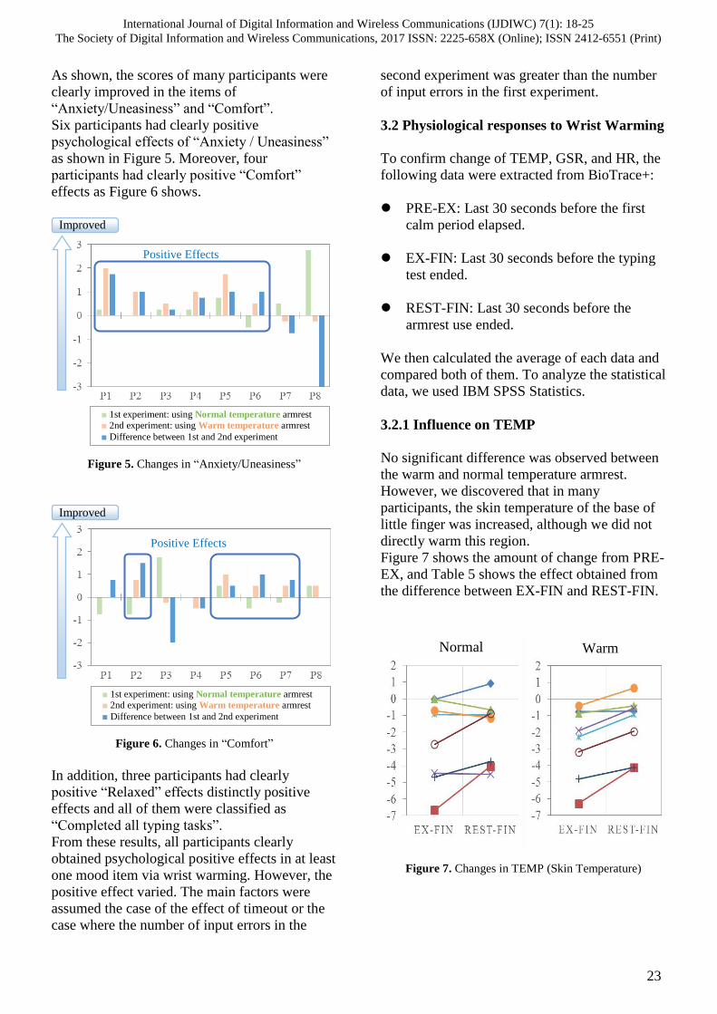
As shown, the scores of many participants were
clearly improved in the items of
“Anxiety/Uneasiness” and “Comfort”.
Six participants had clearly positive
psychological effects of “Anxiety / Uneasiness”
as shown in Figure 5. Moreover, four
participants had clearly positive “Comfort”
effects as Figure 6 shows.
Figure 5. Changes in “Anxiety/Uneasiness”
Figure 6. Changes in “Comfort”
In addition, three participants had clearly
positive “Relaxed” effects distinctly positive
effects and all of them were classified as
“Completed all typing tasks”.
From these results, all participants clearly
obtained psychological positive effects in at least
one mood item via wrist warming. However, the
positive effect varied. The main factors were
assumed the case of the effect of timeout or the
case where the number of input errors in the
second experiment was greater than the number
of input errors in the first experiment.
3.2 Physiological responses to Wrist Warming
To confirm change of TEMP, GSR, and HR, the
following data were extracted from BioTrace+:
PRE-EX: Last 30 seconds before the first
calm period elapsed.
EX-FIN: Last 30 seconds before the typing
test ended.
REST-FIN: Last 30 seconds before the
armrest use ended.
We then calculated the average of each data and
compared both of them. To analyze the statistical
data, we used IBM SPSS Statistics.
3.2.1 Influence on TEMP
No significant difference was observed between
the warm and normal temperature armrest.
However, we discovered that in many
participants, the skin temperature of the base of
little finger was increased, although we did not
directly warm this region.
Figure 7 shows the amount of change from PRE-
EX, and Table 5 shows the effect obtained from
the difference between EX-FIN and REST-FIN.
Figure 7. Changes in TEMP (Skin Temperature)
Normal Warm
Positive Effects
Improved
■ 1st experiment: using Normal temperature armrest ■ 2nd experiment: using Warm temperature armrest
■ Difference between 1st and 2nd experiment
Improved
Positive Effects
■ 1st experiment: using Normal temperature armrest ■ 2nd experiment: using Warm temperature armrest
■ Difference between 1st and 2nd experiment
International Journal of Digital Information and Wireless Communications (IJDIWC) 7(1): 18-25The Society of Digital Information and Wireless Communications, 2017 ISSN: 2225-658X (Online); ISSN 2412-6551 (Print)
23

Table 5. Effects of TEMP (Skin Temperature)
P1 P2 P3 P4 P5 P6 P7 P8
Normal
○ ○○ × × × × ○○ ○○
Warm
△ ○○ ○ ○○ ○○ ○○ ○○ ○○
From the result, the finger skin temperature
(TEMP) increased for many participants via
wrist warming. Therefore, it is possible that they
experienced stress relief by wrist warming.
Moreover, there is a high possibility that they
obtained these stress relieving effects by the
warming of their fingers whose temperatures had
decreased because of the mental workload.
3.2.2 Influence on GSR
Wrist warming decreased GSR for some
participants. However, many of them had the
result of their GSR decreased in normal
temperature armrest than in wrist warming.
Figure 8 shows amount of change from PRE-EX,
and Table 6 shows the effect obtained from the
difference between EX-FIN and REST-FIN.
Figure 8. Changes of GSR
Table 6. Effects of GSR
P1 P2 P3 P4 P5 P6 P7 P8
Normal
○○ ○○ ○ ○ ○○ △ ○○ ○
Warm
○ ○ × × △ ○ ○○ ○
From the result, it seems possible that increased
finger skin temperature by wrist warming
increases GSR. Therefore, it seems possible that
the sensors could not accurately detect the stress
relieving effects of wrist warming.
3.2.3 Influence on HR
Figure 9 shows EX-FIN and REST-FIN for HR,
and Table 7 shows the effect obtained from the
reduction rate between EX-FIN and REST-FIN.
In this result, no significant difference was
detected between the warm and normal armrests.
Figure 9. Changes in HR
Table 7. Effects of HR
P1 P2 P3 P4 P5 P6 P7 P8
Normal
○○ ○○ ○○ * ○○ ○ ○○ ○
Warm
○ ○○ ○ * △ ○ ○○ ○○
[○○] : Significantlydecreased (>1 )
[ ○] : Decreased (>0.5)
[ △] : Decreased slightly (>0)
[ ×] : Not Decreased
Normal Warm
*The data of 1 participant was excluded because of sensor measurement error
*1 participant data was excluded cause by sensor measurement error
[○○] : Significantly decreased (>10%)
[ ○] : Decreased (>5%)
[ △] : Slightly decreased (>0%)
[○○] : Significantly increased (>1 )
[ ○] : Increased (>0.5)
[ △] : Increased slightly (>0)
[ ×] : Not Increased
Normal Warm
International Journal of Digital Information and Wireless Communications (IJDIWC) 7(1): 18-25The Society of Digital Information and Wireless Communications, 2017 ISSN: 2225-658X (Online); ISSN 2412-6551 (Print)
24

In this experiment, we had measured ECG data
from both arms of each participant.
1 participant could not detect normal heart rate
because of interference by muscular motion.
Moreover, it seemed possible that other
participants HR data had some influence due to
same reason.
4 CONCLUSION
In this study, we researched the psychological
and physiological responses to wrists warming
after mental workload from a timed typing test.
Psychological responses were evaluated with a
21 questionnaire items with 7 mood state
categories.
Physiological responses were evaluated with
changes in the heart rate, skin temperature and
galvanic skin temperature.
We conducted an experiment involving 8 healthy
participants.
Considering the results, wrist warming after
mental workload may result in mental stress
relief. This is because participants had clearly
improved moods of “Anxiety/Uneasiness” and
“Comfort” due to the temperature rise of their
fingers.
On the other hand, it is possible that wrist
warming could bring a few positive effects for
people under intense stress.
In the future, to clarify the mental stress relief
effects of wrists warming, the impact of
differences in personality should be elucidated.
We will research it by using additionally
physiological responses such as heart rate
variation.
Moreover, we will research the impact of wrist
warming as a new relief method in the office
after implementing mental workload.
REFERENCES 1. K. Kato, “Properties of Pleasure Using Hot Back-
Compresses : Changes in Pleasure-Displeasure and Autonomic Nerve Activity after the Uchida-Kraepelin Stress Test, ” Japanese Journal of Nursing Art and Science Vol. 9, No. 2, pp 4–13, 2010
2. K. Kaneko, Y. Ogata, H. Kumagai, M. Yamamoto, “Physiological Effects of Hot Compresses to Foot with Steamed Towel : Comparison with Footbath Uses on Cardiovascular Dynamics and Autonomic Nervous Functions, ” Japanese Journal of Nursing Art and Science Vol. 11, No. 2, pp4-11, 2012
3. The Ministry of Health, Labour and Welfare, “Guidelines for Industrial Health Controls of VDT Operations,” Japan Kihatsu No. 0405001, April 5, 2002.
4. M. Suzuki, N. Hirano, H. Terashita, Y. Oda and A. Yagi, “On the items and usage of a questionnaire for evaluation of stress caused by phasic task demand,” Japan Ergonomics Society vol 35(4), pp.259-270, 1999.
5. A. Sato, and A. Yasuda, “Development of the Japanese version of Positive and Negative Affect Schedule (PANAS) scales,” Japan Society of Personality Psychology vol. 9(2), pp.138-139, 2001-03-30.
6. K. Hashimoto, M.Murakami, “Reliability and validity
of the reversed Mood Check List-short form 2 (MCL-
S.2) measuring the positive mood state following
exercise,” Jounal of Health Science, Kyusyu
University, Vol.33, pp.21-26,2011
International Journal of Digital Information and Wireless Communications (IJDIWC) 7(1): 18-25The Society of Digital Information and Wireless Communications, 2017 ISSN: 2225-658X (Online); ISSN 2412-6551 (Print)
25

Takahiro Suzuki
Faculty of Science and Engineering,
Hosei University, Kajino-cho 3-7-2, Koganei-shi,
Tokyo 184-8584
Shihoko Tanabe
Faculty of Science and Engineering,
Hosei University Kajino-cho 3-7-2, Koganei-shi,
Tokyo 184-8584
Isamu Shioya
Faculty of Science and Engineering,
Hosei University Kajino-cho 3-7-2, Koganei-shi,
Tokyo 184-8584
ABSTRACT
This paper presents an acceleration model of traffic re-
source utilization from psychological effects of car drivers
on a single lane traffic resource. Two kinds of acceleration,
boundary and fluctuation effects, which are of drivers ef-
fects are considered. The boundary effect, which is based
on a hard sphere model, is an interaction that drivers feel
the pressure from other cars in front or behind. The fluctu-
ation effect, which can achieve the higher resource utiliza-
tion in a hard sphere model, is to accelerate or reduce car
speed randomly. The two effects are closely related to how
we drive a car in highway traffic. We introduce several
types of drivers depending on the two effects combined
with two car moving types: a fast moving and a sure mov-
ing. We finally examine the traffic flow features, which
include phase transitions, among their types of drivers by
computer simulation.
KEYWORDS
Traffic resource acceleration, moving multi-agents, psy-
chological effects and phase transitions.
1 INTRODUCTION
In this paper, we present an acceleration model of
traffic resource utilization from psychological effects
of car drivers on a single lane traffic resource. Two
kinds of acceleration, boundary and fluctuation ef-
fects, which are of drivers effects are considered. The
boundary effect[8], which is based on a hard sphere
model, is an interaction that drivers feel the pressure
from other cars in front or behind, and it keeps cars
safe during car driving. The fluctuation effect[8],
which can achieve the higher resource utilization in
a hard sphere model, is to accelerate or reduce car
speed randomly. Their effects are closely related to
how we drive a car in highway traffic. We introduce
several types of drivers depending on two effects, the
boundary and fluctuation effects, which are combined
with two car moving types: a fast moving and a sure
moving. We finally examine the traffic flow features,
which include phase transitions, among their types of
drivers considering two kinds of the acceleration by
computer simulation.
A traffic congestion is a big problem in the world,
and a huge amount of energy has been consumed
since the 20th century. It may be difficult to prevent a
traffic congestion, because a traffic resource is finite,
and a huge number of cars are flooded in the traf-
fic resource, but it is concentrated in very local traffic
rather than everywhere, so that we believe that we can
find out the solutions to resolve it. A difficult prob-
lem is that the space of traffic problems belongs to
high dimensional spaces rather than four dimensions,
because each car autonomously runs around a traffic
almost freely. That is, it is one of autonomous multi-
agent problems. On the other hand, a car driving is
sort of stressful work. Suppose that you are now driv-
ing a car in highways. You may feel a lot of psycho-
logical stress to drive a car safely, when other cars are
running in front or behind of your car. Then, you may
accelerate/reduce the car speed as a driver reaction,
and we call it a boundary effect. In another case, you
may be difficult to keep a car speed constant during
running cars, because of uphills, downhills, human
factors or others, i.e. even if there are no interactions
with other cars, the speed of your car would be also
accelerated/reduced as a driver reaction, and we call
it a fluctuation effect. Our problem is to present how
boundary and fluctuation effects are related to a traffic
flow.
A variety of different traffic flow models have been
presented for analyzing a traffic flow and finding the
Accelerated Traffic Model based on Psychological Effects
International Journal of Digital Information and Wireless Communications (IJDIWC) 7(1): 26-34The Society of Digital Information and Wireless Communications, 2017 ISSN: 2225-658X (Online); ISSN 2412-6551 (Print)
26
solutions of traffic congestion. There are two kinds
of models to discuss a traffic flow: macro and micro
models. A typical one of the macro model is based on
Burgers equation from fluid mechanics[5]. The other
micro model can be divided into two classes: Opti-
mal Velocity (OV) model[1] and Cellular Automaton
(CA) model [3]. OV model is presented for explain-
ing traffic congestion based on differential equations.
CA model [3] is successfully presented a fundamen-
tal model based on CA to reproduce traffic flow faith-
fully. But, it is sometimes difficult to explain why
the model is successful. This paper discusses a traffic
flow based on driver reactions including psychologi-
cal human factors, and clarifies how the driver reac-
tions are related to a traffic flow.
The works [4, 6] based on a probabilistic cellular
automaton model employed some rules, which are
similar to this paper, on a circle rather than our model
discussed on a straight line: acceleration, slowing-
down, randomization and car motion rules, and the
model is trying to reproduce fairly faithfully a traffic
flow in highways. The work [2] which employed a
slow-to-stop rule indicates that the results are close to
a actual traffic flow.
A traffic flow is mainly determined from two kinds
of features: “drivers effects including the interaction
between cars” and “the unique feature of a traffic in-
cluding time lags”. A driver is sometimes difficult to
keep the speed of a car constant so that the fluctuation
effect is to accelerate or slow down the car speed ran-
domly. We presented a basic driver’s model based on
cellular automaton(CA) with the two effects[10], and
examined the unique feature, phase transitions, of the
model.
Our motivation of this paper is that a traffic flow is a
stochastic autonomous moving multi-agent from the
viewpoint of the efficient uses of traffic resources in
moving multi-agent systems[7], the behavior of the
multi-agents is complicated, each car is an agent in
multi-agents, and each agent is arranged on the cells
exclusively. Then, the fluctuation and boundary ef-
fects play important roles to achieve high resource
utilization.
A lot of traditional traffic flow work mainly con-
centrate to reproduce a real traffic flow phenomena
in computers, and they mostly use a fundamental dia-
gram to check whether or not a proposed traffic model
is consistent with a real traffic flow. Actually, a traf-
fic flow feature greatly depends on how drivers run
traffic, even if the traffic is a highway. There are two
kinds of extreme car moving types: fast moving andsure moving[10]. The fast moving is an ideal typeof car moving without time lags to move a car in a
traffic. Therefore, when the speed of all the cars are
greater than or equal to 1, every cars can move to for-ward at least one cell at the same time by one time
step in CA. It is true even if all the cells are occupied
by cars. That is, the cell updates in CA are performed
from the most forward cell to backward cell, sequen-
tially. So they can be performed in one time step, and
we can say that there are no time lags to move a car
in fast moving.
On the other hand, sure moving[4] is a type of a safecar moving at the next cell time step, and a car can
move to forward, only if there are no cars in ahead
at the previous time step. In other words, the sure
moving is a fast moving with time lags. So, it can be
performed by parallel cell updates in sure moving. A
real car moving in highways is the probabilistic mix-
ture of the two kinds of moving types with inertia.
However, we do not consider an inertia in this paper.
Why not consider an inertia? An inertia in a real traf-
fic makes the traffic flow features invisible so that we
can not see the phenomena well. Actually, the dis-
tinctive phase transitions are visible in an ideal traf-
fic flow[10]. We expect the usefulness in a dynami-
cal traffic environment. Also, an autonomous driving
may make this work valuable in future.
The paper[10] only discussed the fast movingwhich is an ideal maximum traffic flow without time
lags from the drivers view in a single traffic, and the
model achieves higher traffic resource utilization by
considering boundary and fluctuation effects. Then,
six types of drivers introduced: nb-nf, nb-f, b-nf, b-
nf-a, b-f, b-f-a, and their probabilistic combinations,
where they do not consider the time lags and/or iner-
tia, and we presented phase transitions by varying the
types to drive a car. The model sounds the case where
there is no time lags and no inertia.
Our model is an extension of a moving multi-agent
in a hard particle model on closed regions[7, 9] to
a traffic flow. We note that the model[7] is distinct
from [10]. [7] is not an ASEP(Asymmetric Simple
Exclusion Process), whereas [10] is a TASEP(Totally
Asymmetric Simple Exclusion Process). But, one of
their common features is to achieve the efficient use
of resources by an acceleration. The acceleration is
composed from the above two effects. The two effects
are not only closely related to how we drive a car[10],
but the paper also presented a solution for achieving
higher resource utilization. It is amenable to a traffic
driver model based on stochastic cellular automaton,
and natural to reproduce a traffic flow more faithfully.
The main contribution of this paper is to see the
traffic flow from two kinds of psychological aspects
in the efficient uses of traffic resources, boundary and
fluctuation effects combined with car moving types:
fast moving and sure moving. The boundary effects
International Journal of Digital Information and Wireless Communications (IJDIWC) 7(1): 26-34The Society of Digital Information and Wireless Communications, 2017 ISSN: 2225-658X (Online); ISSN 2412-6551 (Print)
27

are an essential nature of traffic flow, and are related
to a transportation system. Our traffic cell updates are
performed by two kinds of car movings, which are an
ideal traffic flow considering time lags/no time lags
to move a car. In fast moving, the cell updates are
performed from right to left sequentially rather than
parallel of sure moving. The fluctuation effects are re-
lated to driving types which due to drivers, so that the
car speed is not only randomly changed by drivers but
also the average car moving speed is randomly shifted
to either slower or faster. We show how the boundary
and fluctuation effects are related to traffic congestion
to be happened in highways under two kinds of car
moving types: fast car moving and sure car moving.
This paper is organized as: the following section
presents our proposal traffic flowmodel and discusses
it. Section 3 shows our experimental results. In the
final Section 4, we conclude this paper.
2 TRAFFIC FLOWMODEL BASED ON PSY-CHOLOGICAL EFFECTS
We assume a stochastic traffic flow cell model whose
cells are arranged over a traffic resource, and the traf-
fic is a one-way lane (Figure 1 and 2). Each cell of
the traffic is occupied by a car at most, and every cars
stochastically run on the traffic resource from left to
right.
�
� � �����
Figure 1. One-way traffic resources, and cars can run from left
to right.
���������������
��� ��������� ������� ������� �
����
Figure 2. The traffic flow in time domain.
Assume that the speed of each moving car is always
changed at every time steps stochastically, and it de-
pends on traffic rules, car performance, traffic flow
and driver effects. Suppose you are driving a car in
��� ���� ���
������
���
��� ���� ���
������
���
Figure 3. Slower-in: Boundary effects in front.
������ �
��� ���
���
Figure 4. Go-faster: Boundary effects behind.
highways. We consider the driver types as the fol-lowing:
1. If a slower moving car (the car (b) in Figure 3)
in front of your car is running, you (the car (a)
in Figure 3) may slow down the speed more than
necessaries in advance so that you might allevi-
ate the psychological stress by slower-in and it
becomes more safe. This is one of driver types.
On the other hand, if there is also another car (the
car (b) in Figure 4) behind and there are no cars
in ahead, the speed of your car (the car (a) in
Figure 4) might be accelerated for avoiding from
psychological stress behind, that is go-faster or
faster-out. This is also one of driver types. In
this paper, the driver types that change the speed
more than necessaries for avoiding collisions or
alleviating a lot of psychological stress are said
to be boundary effects. They depend on othercars stochastically.
2. As a special case of the boundary effects in
above, if the cell in front of your car is unoc-
cupied, but the second cell in ahead and the cell
in behind are occupied, your car is either shorten
one cell in front (see the car (a) in Figure 5) or
not shorten, i.e. you either move a cell in ahead
or remain there. Therefore, we need a conflict
resolution of it, and we say it a minimal bound-ary effect.
3. Also, if there are small uphills or downhills in
highways (Figure 6), you would be difficult to
keep the car speed constant, and the speed of
your car will be accelerated/slowed down in av-
erage speed. These also arise from some reasons
including human factors or others, and do not
depend on other cars. We say that their driver
effects are fluctuation that the average moving� ������
���
���
� ������
���
���
Figure 5. Shortening one cell too close a car in front in minimum
boundary effects.
International Journal of Digital Information and Wireless Communications (IJDIWC) 7(1): 26-34The Society of Digital Information and Wireless Communications, 2017 ISSN: 2225-658X (Online); ISSN 2412-6551 (Print)
28

Figure 6. An uphill in fluctuation effects.
speed of cars is randomly shifted to either faster
or slower rather than a randomization[4].
Now, how are you driving a car? We can consider
two extreme car moving types in a traffic flow: “Fast
moving” and “Sure moving”. “Fast moving” is an
ideal type of fast car moving in a traffic, so there are
no time lags to move a car. Therefore, when the speed
of all the cars are greater than or equal to 1, every carcan move to forward at the same time by one step in
CA, even if all the cells are occupied by a car. That is,
the updates in CA are performed from the most right
cell to left cell, sequentially.
On the other hand, “Sure moving” is a type of a safe
car moving at the next update step, so a car can move
to forward, only if there are no cars in ahead at the
previous time step. Actual car moving in highways
is the probabilistic mixture of two kinds of moving
types: fast moving and sure moving.
���� ���
���� ���
������
������
���� ���������
���� ��������
���� ��������
���� ���������
�
�
���
�
�
���
���
Figure 7. Six cases of driving in our traffic model.
We consider six car driving types based on the
driver effects shown in Table 1, and assign the sym-
bols nb-nf,.., and b-f-a to their driving types. We also
assign the symbols to their driver’s types in conjunc-
tion with moving types as shown in Table 2.
We can consider several cases to run a traffic as
shown in Figure 7. The outline of our algorithm is
given as the following: Suppose a car is running on a
traffic.
1. Minimum boundary effect: If the car runsin minimum boundary effect, it may be either
shorten or not shorten. If it is true and the car
speed is not zero, the car moves to the next cell.
Otherwise, it will stay there.
2. Backward boundary effect: If the car runs inbackward boundary effect, the car speed is in-
creased.
3. Forward boundary effect: If the car runs in for-ward boundary effect, the car speed is decreased.
4. Fluctuation effect: The average car speed
increases/decreases in averages with the speci-
fied probability.
5. Otherwise: The car moves to forward by givenspeed.
Table 1. Driver’s types.
nb-nf neither boundary nor fluctuation.
nb-f allow fluctuation, but no boundary.
b-nf allow boundary, but no fluctuation,
no shorten in minimum boundary.
b-nf-a allow boundary, but no fluctuation,
shorten one cell in minimum boundary.
b-f allow both boundary and fluctuation,
no shorten in minimum boundary.
b-f-a allow both boundary and fluctuation,
shorten one cell in minimum boundary.
Table 2. The driver’s types in conjunction with moving types.
fast moving sure moving
f-nb-nf s-nb-nf
f-nb-f s-nb-f
f-b-nf s-b-nf
f-b-nf-a s-b-nf-a
f-b-f s-bf
f-b-f-a s-b-f-a
The speed of each car at every time steps is stochas-
tic, and we assume that it, the speed of all the cars,
has the same probability density distribution f(x) inthe cases without driver effects. But, the form of
f(x) varies diverse if there are driver effects. Wecan consider that a traffic is one of stochastic moving
multi-agents with exclusive resource sharing: each
cell is occupied by a car at most, and a traffic flow
is a behavior of the multi-agents whose agents are
arranged on a straight line consisting of traffic cells.
Our driver effects provide the interaction between two
agents, but no direct interactions among more than
three agents.
In the following section, our experiments show how
the driver effects are related to the traffic flow in two
moving types.
International Journal of Digital Information and Wireless Communications (IJDIWC) 7(1): 26-34The Society of Digital Information and Wireless Communications, 2017 ISSN: 2225-658X (Online); ISSN 2412-6551 (Print)
29

3 EXPERIMENTS
We consider six car driving types based on the driver
reactions in Section 2, shows them in Table 1, and
assign the symbols nb-nf,.., and b-f-a to their driving
types.
We prepare a one-way traffic consisting cells, and
the traffic is one lane. Every car moves on the traffic
cells from left to right shown in Figure 1. The num-
ber of the traffic cells is 2, 000. The moving type isfast moving, so we perform the updates of the traffic
cells from right to left, reverse, at each moving step,
and provide 20, 000 cars. Their cars run 20, 000 stepsfor each exam in our experiments. At each updating
step, a car enters into the traffic only if the leftmost
traffic cell is empty. Otherwise, the car has to wait
to enter into the traffic until left most cell becomes
empty. This means that we examine the maximum
traffic flow for every driving type in fast moving.
Each car speed randomly changes at every moving
step. We use Mersenne twister as a random number
generator. Then, each car speed v is either 0, 1, 2, 3or 4 in the cases without driver effects, and the distri-
bution of their speed is given by 0, 1/16, 14/16, 1/16and 0 in this examination. So the average value is 2 ifthere are no effects.
The boundary effects are implemented as every car
speed v either increase 1 in average if the behind cellis occupied and two more cells in ahead are unoccu-
pied, or decrease 1 in average if v more cells in aheadare unoccupied and the car approaches the behind of
a car in ahead with lower speed. Shortening one cell
in the minimal boundary effect (Figure 5) is consid-
ered if there only exists an empty cell in front and the
speed is greater than or equal to 1. With even proba-
bility, the fluctuation effects either increase the speed
1 or decrease the speed 1 in average.We examine the car density and the traffic flow by
varying the distributions of the speed for every exam
(Table 3). Then, we observe the car density on the
cells between 501th and 1,500th, and the traffic flow
is the number of cars to pass on the 2,000th cell be-
tween 10,001th and 20,000th steps. We repeat 10
times for each driving type.
We obtained the traffic flow versus car density rela-
tionships shown in Figure 8-13. The probability dis-
tribution of each car speed is shown in Table 3. In
Figure 8, the car speed splits into either low or high.
Then, the traffic flow and car density are low in both
in the car driving type b-f. If we disallow fluctua-
tion effects and allow to shorten one cell in minimum
boundary, that is b-nf-a, the traffic flow and car den-
sity become high in both.
In Figure 9, the probabilities of each speed are al-
most even, i.e. the distribution of it is almost flat.
Then, the traffic flow versus car density relationship
has moved to the right upside. But, the traffic flow
and car density are low in both in b-f. The similar
trend is seen in Figure 10. When the speed distri-
bution is sharpened more slightly (Figure 11), b-nf-a
turns to left upside, and others are moving toward the
upside. Furthermore, a little more sharped case of the
speed distribution is shown in Figure 12. The Figure
13 shows the most sharpened case. There, the traffic
flow and car density are still low in both in b-f. b-nf-
a, b-nf and nb-nf, and they are coming together to the
middle of upside. On the other hand, b-f-a moved to
left upside. We examined the difference between n-
nf-a and b-f-a in Figure 14. The more detail is shown
in Figure 15. The difference between two is only fluc-
tuation effects. Both are almost the same traffic flow,
but quit different in car density. So, we gradually
change the event probabilities of the fluctuation ef-
fects between b-nf-a and b-f-a. res-f-00-16-00 repre-
sents that there are no fluctuation effects. res-f-01-14-
01 represents that it increases the speed 1 in average
with probability 116, and it decreases the speed 1 in
average with probability 116. Otherwise, there are no
fluctuations. Similarly, res-f-08-00-08 represents that
it increases the speed 1 in average with probability 816,
and it decreases the speed 1 in average with probabil-
ity 816. Then, the traffic flow of res-f-03-10-03 and
res-f-04-08-04 has remained in a small change, while
their car densities are quit distinct. It works like a
switch in electrical circuits. Figure 16 shows the case
that every car speed is 2, while it allows the mini-
mum boundary effects. By changing the distribution
of fluctuation effects, we can see that the traffic flow
keeps higher while the car densities are changed dras-
tically.
Figure 21 shows how boundary effects are related
to fluctuation effects, so that both boundary and fluc-
tuation effects are of essential to achieve efficient uti-
lization of traffic resources, where b, f and d repre-sent the probabilities of boundary effect, the std. de-
viation of fluctuation effect and car density on cells,
respectively. Our results show that we feel stress in
driving and take some actions as driver reactions so
that the car density in traffic flow is improved drasti-
cally. The figure in Figure 22 shows the number of
traffic flow varying the probability of boundary and
fluctuation effects in two dimensional space, where vrepresents the number of cars to pass. Then, the car
density becomes higher in fast moving and minimum
boundary.
The figures in Figure 17 and 18 present the car den-
sity and the number of traffic flow. Then, the mixture
of fast moving and sure moving with probability 0.5,
International Journal of Digital Information and Wireless Communications (IJDIWC) 7(1): 26-34The Society of Digital Information and Wireless Communications, 2017 ISSN: 2225-658X (Online); ISSN 2412-6551 (Print)
30
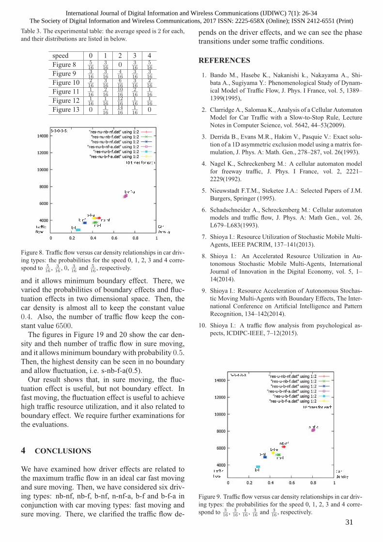
Table 3. The experimental table: the average speed is 2 for each,and their distributions are listed in below.
speed 0 1 2 3 4
Figure 8 516
316 0 3
16516
Figure 9 316
316
416
316
316
Figure 10 216
316
616
316
216
Figure 11 116
216
1016
216
116
Figure 12 116
116
1216
116
116
Figure 13 0 116
1416
116 0
����������
�����
�����
�������
����
����
��� �����������
��
���� ��
���� �
����
Figure 8. Traffic flow versus car density relationships in car driv-
ing types: the probabilities for the speed 0, 1, 2, 3 and 4 corre-
spond to 516 ,
316 , 0,
316 and
516 , respectively.
and it allows minimum boundary effect. There, we
varied the probabilities of boundary effects and fluc-
tuation effects in two dimensional space. Then, the
car density is almost all to keep the constant value
0.4. Also, the number of traffic flow keep the con-stant value 6500.The figures in Figure 19 and 20 show the car den-
sity and theh number of traffic flow in sure moving,
and it allows minimum boundary with probability 0.5.Then, the highest density can be seen in no boundary
and allow fluctuation, i.e. s-nb-f-a(0.5).
Our result shows that, in sure moving, the fluc-
tuation effect is useful, but not boundary effect. In
fast moving, the fluctuation effect is useful to achieve
high traffic resource utilization, and it also related to
boundary effect. We require further examinations for
the evaluations.
4 CONCLUSIONS
We have examined how driver effects are related to
the maximum traffic flow in an ideal car fast moving
and sure moving. Then, we have considered six driv-
ing types: nb-nf, nb-f, b-nf, n-nf-a, b-f and b-f-a in
conjunction with car moving types: fast moving and
sure moving. There, we clarified the traffic flow de-
pends on the driver effects, and we can see the phase
transitions under some traffic conditions.
REFERENCES
1. Bando M., Hasebe K., Nakanishi k., Nakayama A., Shi-
bata A., Sugiyama Y.: Phenomenological Study of Dynam-
ical Model of Traffic Flow, J. Phys. I France, vol. 5, 1389–
1399(1995),
2. Clarridge A., Salomaa K., Analysis of a Cellular Automaton
Model for Car Traffic with a Slow-to-Stop Rule, Lecture
Notes in Computer Science, vol. 5642, 44–53(2009).
3. Derrida B., Evans M.R., Hakim V., Pasquie V.: Exact solu-
tion of a 1D asymmetric exclusion model using a matrix for-
mulation, J. Phys. A: Math. Gen., 278–287, vol. 26(1993).
4. Nagel K., Schreckenberg M.: A cellular automaton model
for freeway traffic, J. Phys. I France, vol. 2, 2221–
2229(1992).
5. Nieuwstadt F.T.M., Steketee J.A.: Selected Papers of J.M.
Burgers, Springer (1995).
6. Schadschneider A., Schreckenberg M.: Cellular automaton
models and traffic flow, J. Phys. A: Math Gen., vol. 26,
L679–L683(1993).
7. Shioya I.: Resource Utilization of Stochastic Mobile Multi-
Agents, IEEE PACRIM, 137–141(2013).
8. Shioya I.: An Accelerated Resource Utilization in Au-
tonomous Stochastic Mobile Multi-Agents, International
Journal of Innovation in the Digital Economy, vol. 5, 1–
14(2014).
9. Shioya I.: Resource Acceleration of Autonomous Stochas-
tic Moving Multi-Agents with Boundary Effects, The Inter-
national Conference on Artificial Intelligence and Pattern
Recognition, 134–142(2014).
10. Shioya I.: A traffic flow analysis from psychological as-
pects, ICDIPC-IEEE, 7–12(2015).
������
�����
���
��������
�����
���
����
�������
����
��������������
���������
Figure 9. Traffic flow versus car density relationships in car driv-
ing types: the probabilities for the speed 0, 1, 2, 3 and 4 corre-
spond to 316 ,
316 ,
416 ,
316 and
316 , respectively.
International Journal of Digital Information and Wireless Communications (IJDIWC) 7(1): 26-34The Society of Digital Information and Wireless Communications, 2017 ISSN: 2225-658X (Online); ISSN 2412-6551 (Print)
31
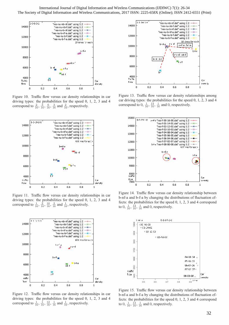
���������
������
�����
���
����
���� �����
�� ������������
���
���� ��
����� �
����
Figure 10. Traffic flow versus car density relationships in car
driving types: the probabilities for the speed 0, 1, 2, 3 and 4
correspond to 216 ,
316 ,
616 ,
316 and
216 , respectively.
������
�����
���
����
����
�����
����� ���������
���
��� �
����������
������
����
Figure 11. Traffic flow versus car density relationships in car
driving types: the probabilities for the speed 0, 1, 2, 3 and 4
correspond to 116 ,
216 ,
1016 ,
216 and
116 , respectively.
����������
�����������
���
����
����
�����
���� ���� ���
���
� ����
�������
����
Figure 12. Traffic flow versus car density relationships in car
driving types: the probabilities for the speed 0, 1, 2, 3 and 4
correspond to 116 ,
116 ,
1216 ,
116 and
116 , respectively.
����������
������
�����
���������������
���� ���
���
�����
����
����� ����
���� ���������
���
�������
�������
����
Figure 13. Traffic flow versus car density relationships among
car driving types: the probabilities for the speed 0, 1, 2, 3 and 4
correspond to 0, 116 ,
1416 ,
116 and 0, respectively.
����������
������
�����
���� ���� ���
���
� ����
�������
����
�����
������
Figure 14. Traffic flow versus car density relationship between
b-nf-a and b-f-a by changing the distributions of fluctuation ef-
fects: the probabilities for the speed 0, 1, 2, 3 and 4 correspond
to 0, 116 ,
1416 ,
116 and 0, respectively.
����������������
�����
���������������
�����
��������
��������
� ����
������
�������
�����������
�������
�������
����
Figure 15. Traffic flow versus car density relationship between
b-nf-a and b-f-a by changing the distributions of fluctuation ef-
fects: the probabilities for the speed 0, 1, 2, 3 and 4 correspond
to 0, 116 ,
1416 ,
116 and 0, respectively.
International Journal of Digital Information and Wireless Communications (IJDIWC) 7(1): 26-34The Society of Digital Information and Wireless Communications, 2017 ISSN: 2225-658X (Online); ISSN 2412-6551 (Print)
32
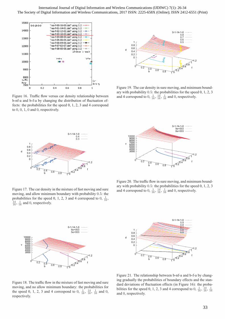
����������
������ �����
���� ���� ���
���
� ����
�������
����
Figure 16. Traffic flow versus car density relationship between
b-nf-a and b-f-a by changing the distribution of fluctuation ef-
fects: the probabilities for the speed 0, 1, 2, 3 and 4 correspond
to 0, 0, 1, 0 and 0, respectively.
0-1-14-1-0 0.4 0.3
0 0.2 0.4 0.6 0.8 1b 0 0.2
0.4 0.6
0.8 1
1.2
f
0 0.2 0.4 0.6 0.8
1
d
Figure 17. The car density in the mixture of fast moving and sure
moving, and allow minimum boundary with probability 0.5: theprobabilities for the speed 0, 1, 2, 3 and 4 correspond to 0, 1
16 ,1416 ,
116 and 0, respectively.
0-1-14-1-0 6e+003 5e+003
0 0.2 0.4 0.6 0.8 1b 0 0.2
0.4 0.6
0.8 1
1.2
f
3000 4000 5000 6000 7000 8000 9000
10000
v
Figure 18. The traffic flow in the mixture of fast moving and sure
moving, and no allow minimum boundary: the probabilities for
the speed 0, 1, 2, 3 and 4 correspond to 0, 116 ,
1416 ,
116 and 0,
respectively.
0-1-14-1-0 0.8 0.7 0.6 0.5
0 0.2 0.4 0.6 0.8 1b 0 0.2
0.4 0.6
0.8 1
1.2
f
0 0.2 0.4 0.6 0.8
1
d
Figure 19. The car density in sure moving, and minimum bound-
ary with probability 0.5: the probabilities for the speed 0, 1, 2, 3and 4 correspond to 0, 1
16 ,1416 ,
116 and 0, respectively.
0-1-14-1-0 9e+003 8e+003
0 0.2 0.4 0.6 0.8 1b 0 0.2
0.4 0.6
0.8 1
1.2
f
3000 4000 5000 6000 7000 8000 9000
10000
v
Figure 20. The traffic flow in sure moving, and minimum bound-
ary with probability 0.5: the probabilities for the speed 0, 1, 2, 3and 4 correspond to 0, 1
16 ,1416 ,
116 and 0, respectively.
0-1-14-1-0 0.9 0.8 0.7 0.6 0.5
0 0.2 0.4 0.6 0.8 1b 0 0.2
0.4 0.6
0.8 1
1.2
f
0 0.2 0.4 0.6 0.8
1
d
Figure 21. The relationship between b-nf-a and b-f-a by chang-
ing gradually the probabilities of boundary effects and the stan-
dard deviations of fluctuation effects (in Figure 16): the proba-
bilities for the speed 0, 1, 2, 3 and 4 correspond to 0, 116 ,
1416 ,
116
and 0, respectively.
International Journal of Digital Information and Wireless Communications (IJDIWC) 7(1): 26-34The Society of Digital Information and Wireless Communications, 2017 ISSN: 2225-658X (Online); ISSN 2412-6551 (Print)
33

0-1-14-1-0
0 0.2 0.4 0.6 0.8 1b 0 0.2
0.4 0.6
0.8 1
1.2
f
3000 4000 5000 6000 7000 8000 9000
10000
v
Figure 22. The traffic flow in fast moving and minimum bound-
ary: the probabilities for the speed 0, 1, 2, 3 and 4 correspond to
0, 116 ,
1416 ,
116 and 0, respectively.
International Journal of Digital Information and Wireless Communications (IJDIWC) 7(1): 26-34The Society of Digital Information and Wireless Communications, 2017 ISSN: 2225-658X (Online); ISSN 2412-6551 (Print)
34

Finding Weak links in Supply chainCase Study: Thai Frozen Shrimp Industry
Patchanee Patitad 1) Hidetsugu Suto1∗) Woramol Chaowarat Watanabe2)1)Graduate school of Engineering, Muroran Institute of Technology
27 Mizumoto-cho, Muroran-shi, Hokkaido, 050-8585 Japan2)School of Logistics and Supply Chain, Naresuan University
99, Moo 9, T. Tha Pho, Muang District, Phitsanulok, 65000 Thailand∗Corresponding author: [email protected]
ABSTRACT
Usually, a manufacture receives materials from one ormore suppliers in a supply chain. Performance of eachsupplier in a chain affects on the chain’s performance.Thus, evaluating suppliers in a supply chain is impor-tant for achieving efficient supply chain. Many meth-ods have already been developed for evaluating per-formance of suppliers. Most of the existing methodsshow us suppliers’ performance, but they do not in-dicate directions for improving supply chains. Withthe proposed method, we can find that which factorsof which suppliers should be improved to achieve ef-ficient condition. Thus, manufacturers can make de-cision for improving or changing suppliers more eas-ily. A case study of Thai frozen shrimp industry isrepresented to show the applicability of the proposedscheme.
KEYWORDS
Data envelopment analysis (DEA), performance mea-surement, multiple suppliers
1 INTRODUCTION
Due to the existing severe competition in businessenvironment, organizations have to improve theirperformance and develop competitiveness [1]. Toachieve improved competitiveness, many manu-facturers have utilized Supply Chain Management(SCM) for increasing their performance [2]. SCMis a principle to manage total flow of distributionchannel from supplier to ultimate customer, in or-der to minimize total cost while satisfying cus-tomer requirements [3]. Efficient supply chainmanagements lead to improve customer value,better utilization of resources, and increased prof-itability [4].Suppliers are considered as important elements ofsupply chain network because their performancesinfluences in the overall chain performance [5].
To obtain efficient supply chain, manufacturershave to choose better suppliers to consist theirsupply chain [6]. However, choosing appropriatesuppliers is difficult because the criteria are mul-tiple and complex. In addition, many qualitativeand quantitative performance indicators should beconsidered such as quality of raw material, price,on time delivery rate, etc [7].Data Envelopment Analysis (DEA) is one of thewell known techniques that is used for evaluatingrelative efficiency of suppliers [8]. DEA has beenapplied in many types of organizations, and somemodified DEA models have been proposed [9].Most of them are designed for evaluating currentperformance of suppliers, and showing improve-ment way is beyond the area of these studies. Inother words, with the traditional DEA models,we can know the efficiency score of a supplier,but we cannot know the strategies to achieve effi-cient situation when it is inefficient [10]. Usually,inefficient chains consist of inefficient suppliers.To increase efficiency of overall performance ofchains, such inefficient suppliers should be im-proved. However, it is difficult that all of the inef-ficient suppliers become efficient because of con-strains of each supplier. Thus, a new method tofind hopeless suppliers which cannot be efficientis proposed. With the proposed method, whichfactors of which suppliers should be improved isclarified. The proposed method can support man-ufacturers’ decision making about managing thesupply chains.In section 2, previous works about supplier perfor-mance measurement in supply chain are shown.Next, the outline of the proposed scheme is de-scribed in section 3. In order to show the useful-ness of the proposed method, Thai frozen shrimpindustry cases are discussed as a case study in sec-tion 4. Finally, results of the proposed scheme arediscussed and concluded in section 5.
International Journal of Digital Information and Wireless Communications (IJDIWC) 7(1): 35-41The Society of Digital Information and Wireless Communications, 2017 ISSN: 2225-658X (Online); ISSN 2412-6551 (Print)
35
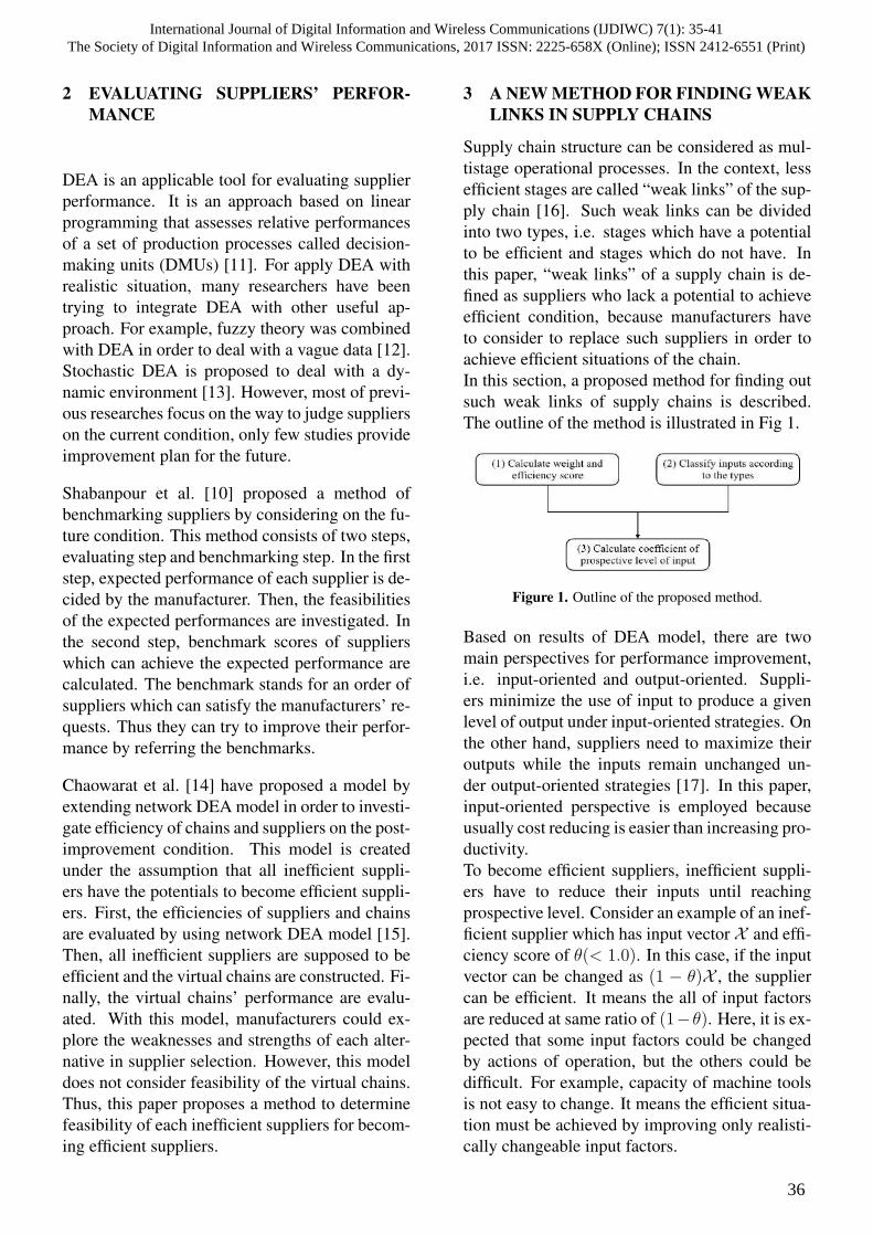
2 EVALUATING SUPPLIERS’ PERFOR-MANCE
DEA is an applicable tool for evaluating supplierperformance. It is an approach based on linearprogramming that assesses relative performancesof a set of production processes called decision-making units (DMUs) [11]. For apply DEA withrealistic situation, many researchers have beentrying to integrate DEA with other useful ap-proach. For example, fuzzy theory was combinedwith DEA in order to deal with a vague data [12].Stochastic DEA is proposed to deal with a dy-namic environment [13]. However, most of previ-ous researches focus on the way to judge supplierson the current condition, only few studies provideimprovement plan for the future.
Shabanpour et al. [10] proposed a method ofbenchmarking suppliers by considering on the fu-ture condition. This method consists of two steps,evaluating step and benchmarking step. In the firststep, expected performance of each supplier is de-cided by the manufacturer. Then, the feasibilitiesof the expected performances are investigated. Inthe second step, benchmark scores of supplierswhich can achieve the expected performance arecalculated. The benchmark stands for an order ofsuppliers which can satisfy the manufacturers’ re-quests. Thus they can try to improve their perfor-mance by referring the benchmarks.
Chaowarat et al. [14] have proposed a model byextending network DEA model in order to investi-gate efficiency of chains and suppliers on the post-improvement condition. This model is createdunder the assumption that all inefficient suppli-ers have the potentials to become efficient suppli-ers. First, the efficiencies of suppliers and chainsare evaluated by using network DEA model [15].Then, all inefficient suppliers are supposed to beefficient and the virtual chains are constructed. Fi-nally, the virtual chains’ performance are evalu-ated. With this model, manufacturers could ex-plore the weaknesses and strengths of each alter-native in supplier selection. However, this modeldoes not consider feasibility of the virtual chains.Thus, this paper proposes a method to determinefeasibility of each inefficient suppliers for becom-ing efficient suppliers.
3 A NEW METHOD FOR FINDING WEAKLINKS IN SUPPLY CHAINS
Supply chain structure can be considered as mul-tistage operational processes. In the context, lessefficient stages are called “weak links” of the sup-ply chain [16]. Such weak links can be dividedinto two types, i.e. stages which have a potentialto be efficient and stages which do not have. Inthis paper, “weak links” of a supply chain is de-fined as suppliers who lack a potential to achieveefficient condition, because manufacturers haveto consider to replace such suppliers in order toachieve efficient situations of the chain.In this section, a proposed method for finding outsuch weak links of supply chains is described.The outline of the method is illustrated in Fig 1.
Figure 1. Outline of the proposed method.
Based on results of DEA model, there are twomain perspectives for performance improvement,i.e. input-oriented and output-oriented. Suppli-ers minimize the use of input to produce a givenlevel of output under input-oriented strategies. Onthe other hand, suppliers need to maximize theiroutputs while the inputs remain unchanged un-der output-oriented strategies [17]. In this paper,input-oriented perspective is employed becauseusually cost reducing is easier than increasing pro-ductivity.To become efficient suppliers, inefficient suppli-ers have to reduce their inputs until reachingprospective level. Consider an example of an inef-ficient supplier which has input vector X and effi-ciency score of θ(< 1.0). In this case, if the inputvector can be changed as (1 − θ)X , the suppliercan be efficient. It means the all of input factorsare reduced at same ratio of (1−θ). Here, it is ex-pected that some input factors could be changedby actions of operation, but the others could bedifficult. For example, capacity of machine toolsis not easy to change. It means the efficient situa-tion must be achieved by improving only realisti-cally changeable input factors.
International Journal of Digital Information and Wireless Communications (IJDIWC) 7(1): 35-41The Society of Digital Information and Wireless Communications, 2017 ISSN: 2225-658X (Online); ISSN 2412-6551 (Print)
36

In order to find enough improvement goal, anequation for calculating coefficient of prospectivelevel of changeable factors is proposed. Manufac-turers can make decision for improving or chang-ing suppliers based on values of coefficient ofprospective level.The steps to find out weak links in supply chainsare described as follows:
Step 1: Calculate weight and efficiency score ofchains and suppliers
In the first step, three kinds of factors that usedto indicate chains’ performance, input, intermedi-ate product and output are determined. The ‘in-put’ means input resources of suppliers. Outputfrom a supplier which enter into the manufacturerare called as ‘intermediate products.’ The ‘output’means final products from the manufacturer.Input i of supplier x in chain j is represented byXx
ij , intermediate product l of supplier x in chainj is represented by Y x
lj , and output k of manufac-turer in chain j is represented by Zkj . Next, dataset of such factors of each member is prepared.After that, weights of each factor and efficiencyscore of each member are calculated by using net-work DEA model shown in section 2.Units which get efficiency score below than oneare considered as inefficient. These inefficientsuppliers should improve their performance.
Step 2: Classify types of inputs
In the second step, inputs are classified into twotypes, i.e. changeable inputs and unchangeableinputs, based on the experiences of the manufac-turer. For instance, inputs come from infrastruc-ture could be classified into unchangeable, and in-puts come from electric power could be classifiedinto changeable.
Step 3: Calculate coefficient of prospectivelevel of changeable inputs
In the third step, coefficient of prospective levelof changeable inputs are calculated by using theequation (1).Coefficient of prospective level indicates ratio be-tween required input and current input. The ra-tio implies possibility that inefficient supplier canbecome efficient. If the coefficient of prospective
level is lower than zero, it means the supplier can-not become efficient by decreasing the changeableinputs.
αS =θS(
∑ni=1 λiXi)−
∑mi=1 λ
ui X
ui∑n−m
i=1 λciX
ci
(1)
Where
αS : Coefficient of prospective level of supplierS
θS : Efficiency score of supplier S
Xi : The i-th input
Xui : The i-th unchangeable input
Xci : The i-th changeable input
λi : Weight of the i-th input
λui : Weight of the i-th unchangeable input
λci : Weight of the i-th changeable input
m : Number of input factors
n : Number of changeable input factors
4 CASE STUDY: THAI FROZEN SHRIMPINDUSTRY
In this section, an example of Thai frozen shrimpindustry is discussed to show the usefulness of theproposed scheme. In this example, fifteen repre-sentative chains are investigated. In these chains,a manufacturer receives fresh shrimps from twosuppliers. Then, the manufacturer processes rawmaterials into frozen shrimp. Finally, the finishedgoods are delivered to the customers. Figure 2shows the structure of the chains.
4.1 Calculate weight and efficiency score ofchains and suppliers (Step1)
The factors that used for indicating performanceare shown in Table 1. The data of each factor hasbeen collected by interviewings. The data sets ofthe chains are shown in Table 2.The weight of each factor and efficiency score ofeach chain were calculated by using network DEAmodel. The results are shown in Table 3 and Ta-ble 4.
International Journal of Digital Information and Wireless Communications (IJDIWC) 7(1): 35-41The Society of Digital Information and Wireless Communications, 2017 ISSN: 2225-658X (Online); ISSN 2412-6551 (Print)
37

Figure 2. Structure of two stage chain with two suppliers and one manufacturer.
Table 1. Performance factors
Construct Factors DescriptionInputs (X) X1: Fixed assets (106 Baht) A long-term tangible property that a organization owns and uses in the
production of its income, e.g. building, machinery,vehicle, etc.X2: Production capacity (kilogram) Volume of products that can be generated by a production plant in a
given period by using current resources.X3: Logistics cost (%) The costs of inventory management and inbound-outbound transporta-
tion over a certain period of time. Typically, inventory cost includescarrying cost, ordering cost and shortage cost.
Intermediate- Y1: Material acceptance rates (%) Percentage of materials being accepted by a manufacturer.product (Y ) Y2: Supplier on-time rate (%) The number of orders that delivered on the requested delivery date
compares with the total number of order.Outputs (Z) Z1: Return on assets Calculated by dividing a company’s annual earning by its total assets.
Z2: Product acceptance rates (%) Percentage of acceptable products by the customers.
The results indicate that there are seven inefficientchains, i.e. chain 5, 6, 7, 8, 11, 12 and 13. Consid-ering efficiency score of supplier1, there are sevenefficient chains, i.e. chain 1, 3, 4, 7, 9, 10 and15. While only four chains that consist of ef-ficient supplier2, i.e. chain 4, 9,14 and 15. Inother words, only chain 4, 9 and 10 consist ofefficient suppliers, and it means only these threechain are good enough in the current stage. Thus,to improve the chains’ performance these ineffi-cient suppliers should be improved.
4.2 Classify types of inputs (Step2)
In this example, each supplier has three input fac-tors, fixed asset, production capacity and logis-tics costs as shown in Table 1. Due to charac-teristic of agricultural production, it is quite diffi-cult to improve fixed asset and production capac-ity. Therefore, we should pay attention to logisticscost. Thus, in this case, logistics costs (X3) areconsidered as changeable input, while fixed assets(X1) and production capacity (X2) are consideredas unchangeable inputs.
4.3 Calculate coefficient of prospective levelof input (Step3)
Coefficient of prospective level of changeable in-put is calculated with the equation (1). Under thecondition of this case, equation for calculating co-efficient of prospective level of changeable inputsis shown as follows:
αS =θS(λ1X1 + λ2X2 + λ3X3)− (λ1X1 + λ2X2)
λ3X3(2)
Where
αS : Coefficient of prospective level of supplierS
θS : Efficiency score of supplier S
X1 : Fixed assets of supplier S (unchangeable)
X2 : Production capacity of supplier S (un-changeable)
X3 : Logistic costs of supplier S (changeable)
λi : Weight of the i-th input of supplier S
International Journal of Digital Information and Wireless Communications (IJDIWC) 7(1): 35-41The Society of Digital Information and Wireless Communications, 2017 ISSN: 2225-658X (Online); ISSN 2412-6551 (Print)
38

Table 2. Data sets of the representative chains in the frozen shrimp industry.
Chain X1 X2 X3 Y1 Y2 Z1 Z2
1 s1 8.21 271.30 42.50 97.14 96.18 0.36 98.53s2 7.49 306.90 42.50 96.63 93.23
2 s1 12.05 306.90 42.50 96.93 95.27 0.66 96.92s2 4.46 271.30 42.50 96.49 92.23
3 s1 12.06 282.80 40.00 97.12 96.03 1.23 98.62s2 6.58 306.90 40.00 95.00 91.88
4 s1 13.40 271.30 45.00 97.62 94.24 2.33 97.65s2 7.67 271.30 43.00 96.00 91.09
5 s1 14.11 373.80 45.00 96.97 95.20 2.72 97.08s2 4.97 373.80 47.00 96.56 91.83
6 s1 16.51 306.90 47.00 98.22 95.57 3.41 97.18s2 5.20 282.80 42.50 96.40 91.68
7 s1 20.37 271.30 42.50 97.69 93.97 3.46 97.74s2 6.00 373.80 45.00 96.62 91.59
8 s1 21.03 373.80 42.50 97.39 94.90 3.97 97.31s2 5.24 282.80 42.50 96.04 91.79
9 s1 24.42 347.30 32.50 97.08 94.39 3.97 98.42s2 4.89 271.30 35.00 96.39 92.29
10 s1 27.87 306.90 35.00 98.04 95.58 4.31 97.45s2 4.68 347.30 40.00 96.91 91.85
11 s1 29.04 309.50 45.00 97.14 95.96 4.71 97.68s2 5.45 306.90 45.00 96.05 91.53
12 s1 29.85 282.80 43.00 97.17 94.71 9.79 98.06s2 4.03 282.80 47.00 95.89 92.34
13 s1 36.59 373.80 42.50 96.96 95.47 10.08 97.61s2 4.00 373.80 42.50 95.57 92.44
14 s1 37.41 282.80 40.00 96.77 95.55 16.86 97.35s2 3.95 309.50 35.00 96.30 91.42
15 s1 38.60 271.30 42.50 97.69 94.41 18.43 98.12s2 3.51 271.30 40.00 96.99 92.45
Coefficient of prospective level of changeable in-puts is shown as α in Table 4.From the table, we can see that chain 12 and chain13 are expected to achieve efficient condition be-cause the suppliers need to decrease their logisticscosts only 20%-6%, and they look realistic goals.The coefficient value of some suppliers are lowerthan zero, i.e. supplier2 of chain 6, supplier2 ofchain 7 and supplier2 of chain 8. It indicates thatthese inefficient suppliers cannot become efficientby decreasing only logistics costs. In this case,the manufacturers should decide to change out thesuppliers. Alternatively, these inefficient suppli-ers should turn to pay attention to improve theirperformance by considering output-oriented per-spective or fundamental investment.
5 DISCUSSION AND CONCLUSION
A new method for finding weak links in sup-ply chains has been proposed. To show the use-fulness of the proposed method, an example ofThai frozen shrimp industry is discussed as a casestudy.With the proposed method, manufacturer can de-cide either requesting inefficient suppliers to im-prove their performances or replacing them byconsidering the value of coefficient of prospectivelevel. This method has been proposed based on aninput-oriented strategy. Sometimes it is difficultto decrease input until input reaches prospectivelevel. Alternatively, inefficient suppliers shouldconsider to improve their performance by consid-
International Journal of Digital Information and Wireless Communications (IJDIWC) 7(1): 35-41The Society of Digital Information and Wireless Communications, 2017 ISSN: 2225-658X (Online); ISSN 2412-6551 (Print)
39

Table 3. Efficiency results of the representative chains infrozen vegetable industry. θAs−is means efficiency score ofchains. θS1 means efficiency score of supplier1. θS2 meansefficiency score of supplier2
Chain θAs−is θS1 θS21 1.000 1.000 0.8842 1.000 0.949 0.9993 1.000 1.000 0.8804 1.000 1.000 1.0005 0.882 0.884 0.8066 0.953 0.902 0.9577 0.994 1.000 0.7918 0.952 0.890 0.9629 1.000 1.000 1.000
10 1.000 1.000 0.92311 0.903 0.904 0.87812 0.968 0.972 0.95913 0.910 0.823 0.92514 1.000 0.996 1.00015 1.000 1.000 1.000
ering output-oriented strategy or fundamental in-vestment. Such cases also be dealt by modifyingthe proposed model as output-oriented strategy.
ACKNOWLEDGMENT
This work was supported by Grants-in-Aidfor Scientific Research from Japan Society forthe Promotion of Science (NO. 15K00486,26350013.)
REFERENCES1. Gunasekaran, A., Patel, C., McGaughey, R.E.: A
framework for supply chain performance measure-ment: International Journal of Production Economics87, 333–347 (2004).
2. Chang, C., Chiang, D.M., Pai, F.: Cooperative strat-egy in supply chain networks: Industrial MarketingManagement 41(7), 1114–1124 (2012).
3. Ellram, L., Cooper, M.: Characteristics of supplychain management and the implications for purchas-ing and logistics strategy: The International Journal ofLogistics Management 4(2), 13–24 (1993).
4. Lee, L.H.:CREATING VALUE through Supply ChainINTEGRATION: Supply Chain Management Review.Peerless Media, (2000).
5. Dweiri, F., Kumar, S., Khan, S.A., Jain, V.: Design-ing an integrated AHP based decision support system
Table 4. Coefficient of prospective level of logistics costsof frozen shrimp industry when considering input-orientedperspective. α means coefficient of prospective level of sup-pliers
Chain λ1 λ2 λ3 α5 s1 2.459 0 6.276 0.870
s2 0 0.3651 2.290 0.5606 s1 0 1.922 6.872 0.723
s2 0 1.557 0.134 -2.3687 s2 0 0.875 0.892 -0.9118 s1 1.726 0 12.780 0.883
s2 0 1.131 0.076 -2.81011 s1 0.641 0 18.748 0.902
s2 0 1.081 7.221 0.75312 s1 0 1.586 20.964 0.958
s2 0.642 0 0.112 0.93913 s1 2.751 0 26.113 0.807
s2 1.35 0 3.476 0.922
for supplier selection in automotive industry: ExpertSystems with Applications 62, 273–283 (2016).
6. Chaowarat, W., Shi, J.: Efficiency measurement ofsupply chain in the export frozen vegetable industry:A network DEA approach: International Journal ofMaterials, Mechanics and Manufacturing 1(1), 88–91(2013).
7. Tseng, M.L., Chiang, J.H., Lan, L.W.:Selection of op-timal supplier in supply chain management strategywith analytic network process and choquet integral:Computers and Industrial Engineering 57(1), 330–340(2009).
8. Azadeh A., Alem, S.M.: A flexible deterministic,stochastic and fuzzy Data Envelopment Analysis ap-proach for supply chain risk and vendor selectionproblem: Simulation analysis: Expert Systems withApplications 37(12), 7438–7448 (2010).
9. Chaowarat, W., Piboonrungroj, P., Shi, J.: A reviewof data development analysis (DEA) applications insupply chain management research. In: Proc. 2013IEEE International Conference on Industrial Engi-neering and Engineering Management, pp. 975–980,IEEE press, New York (2013).
10. Shabanpour, H., Yousefi, S., Saen, R.F.: Future plan-ning for benchmarking and ranking sustainable suppli-ers using goal programming and robust double fron-tiers DEA: Transportation Research Part D: Transportand Environment 50, 129–143 (2017).
11. Cook, W.D., Seiford, L.M.: Data envelopment analy-sis (DEA) - Thirty years on: European Journal of Op-erational Research 192(1), 1–17 (2009).
International Journal of Digital Information and Wireless Communications (IJDIWC) 7(1): 35-41The Society of Digital Information and Wireless Communications, 2017 ISSN: 2225-658X (Online); ISSN 2412-6551 (Print)
40

12. Roshandel, J., Miri-Nargesi, S.S., Hatami-Shirkouhi,L.: Evaluating and selecting the supplier in detergentproduction industry using hierarchical fuzzy TOP-SIS: Applied Mathematical Modelling 37(24), 10170–10181 (2013).
13. Mitropoulos, P., Talias, M.A., Mitropoulos, I.: Com-bining stochastic DEA with Bayesian analysis to ob-tain statistical properties of the efficiency scores: Anapplication to Greek public hospitals: European Jour-nal of Operational Research 243(1), 302–311 (2015).
14. Chaowarat, W., Suto, H., Yokoi, T.: An EvaluationMethod of Supply Chain Efficiency Considering Cus-tomers’ Satisfaction: Transactions of Japan Society ofKansei Engineering 14(1), 231–237 (2015).
15. Chen, C., Yan, H.: Network DEA model for supplychain performance evaluation: European Journal ofOperational Research 213(1), 147–155 (2011).
16. Despotis, D.K., Koronakos, D., Sotiros, D: The“weak-link” approach to network DEA for two-stageprocesses: European Journal of Operational Research254(2), 481–492 (2016).
17. Kao, C., Hwang, S.: Decomposition of technical andscale efficiencies in two-stage production systems:European Journal of Operational Research 211(3),515–519 (2011).
International Journal of Digital Information and Wireless Communications (IJDIWC) 7(1): 35-41The Society of Digital Information and Wireless Communications, 2017 ISSN: 2225-658X (Online); ISSN 2412-6551 (Print)
41

Energy Expenditure Per Bit Minimization Into MB-OFDM UWB Systems
Houda Chihi, Reza Zaeem and Ridha Bouallegue
Innov'Com, Tunis
ABSTRACT
The growing demand of high data rates requires much energy consumption. For this, in this paper we
examine energy efficiency (EE) through total energy
expenditure per bit characterization when the joint coupling between Modulation and Coding Scheme
(MCS) related to the physical layer and Selective
Repeat (SR) truncated Hybrid Automatic Repeat reQuest (HARQ) type I protocol of data link layer is
performed into Multiband Orthogonal Frequency
Division Multiplexing (MB-OFDM) Ultra-Wideband
(UWB) system. The optimization is based on total energy expenditure per bit diminishing constrained
by MCS rate and Packet Error Rate (PER). We
propose an algorithm to identify the optimal MCS rate basing on dichotomy policy. Thus, analytical
analysis highlights a closed-form expression of the
optimal MCS rate allowing energy per bit
minimization. In addition, in measuring the energy consumption per useful information the hardware
components of MB-OFDM UWB (MB-UWB) cross-
layer structure are considered. Further, the analytical framework is validated through computer results
which reveal the effectiveness of our method in terms
of energy saving.
KEYWORDS
Energy per bit minimization; MCS rate; HARQ; MB-OFDM; UWB.
1 INTRODUCTION
The explosive evolution of wireless technologies
yields energy consumption improvement which
implies environmental challenges due to carbon
dioxide (CO2) generation. In that context, EE
appeared as a key metric that needs more
investigation. Indeed, power consumption plays
an interesting role for EE improvement. In this
regard, since UWB systems are recognized by
the important data rates that they provide, EE
should be examined.
In 2002, the Federal Communications
Commission (FCC) [1] allowed a spectrum
range between 3.1 GHz and 10.6 GHz for UWB
system with a Power Spectrum Density (DSP)
about -41.3 dBm/MHz. It was shown that MB-
OFDM solution, standardized by ECMA-368
[2], is an emerging approach enabling high data
rates. For this reason it was chosen as an
efficient candidate for IEEE 802.15.3a channel
[3]. In other side, EE wasn't well investigated
toward MB-UWB systems as power is
distributed identically through sub-bands.
Specifically, the majority of contributions are
interested in physical layer performance
evaluation of the MB-UWB systems. Otherwise,
herein we investigate the combination between
two link adaptation approaches based on MCS of
the physical layer joint with HARQ type I of the
data link layer into the MB-UWB systems. It
should be mentioned that few contributions
discuss link adaptation into MB-UWB systems
[4]. ECMA-368 proposes various data rates for
MB-UWB systems without explaining the
interaction between them. In other side, it should
be mentioned that the combination between
Automatic Repeat reQuest (ARQ) and MCS was
at first the subject of the contribution in [5].
Several contributions have investigated the EE
for instance in [6] where the author examined the
EE in Multi-Input Multi-Output (MIMO)
scenario when ARQ is applied with antenna
selection. In [7] the purpose was about giving
insights according to the EE of both HARQ with
Chase Combining (CC) and Incremental
Redundancy (IR) for Long Term Evolution
(LTE) system following two cases of relaying
applications namely Decode and Forward (DF)
and Amplify and Forward (AF). The authors
analyzed the trade-off between EE and Spectral
Efficiency (SE). In [8] the goal was to
characterize the EE for HARQ mechanism
constrained by statistical buffering. Therefore,
the authors took into consideration the effects of
International Journal of Digital Information and Wireless Communications (IJDIWC) 7(1): 42-48The Society of Digital Information and Wireless Communications, 2017 ISSN: 2225-658X (Online); ISSN 2412-6551 (Print)
42

buffering, deadline and outage probability. The
analysis proposed in [9] compared the EE
between two link adaptation schemes including
AMC and HARQ by using the principle of
Energy Delay Trade-off (EDT) in which
Channel State Information (CSI) was restricted.
The contribution conducted in [10] evaluated
power allocation for HARQ-IR in downlink
scenario under the respect of Quality of Service
(QoS). In addition EE was described in [11]
through power adaptation in various Incremental
Multiple Input Multiple Output (IMIMO)
scenarios based on ARQ, HARQ-CC, and
HARQ-IR where the purpose is to reduce the
outage probability. In [12] it has been reported
three optimization approaches namely energy per
bit reduction, minimizing the normalization
between energy per bit and SE, the trade-off
between EE and SE. The proposed optimization
in [13] was about energy relay determination
allowing throughput maximization through
dichotomy approach. Moreover, the main
concern in our previous work [14] was about EE
improvement by considering MCS scheme only.
In [15], our purpose consisted on minimizing the
energy per throughput into a cross-layer MB-
UWB design. The focus pursued in this
contribution is to determine the efficient MCS
rate allowing energy per bit expenditure
diminishing. Note that the optimization approach
is based on energy per bit minimization
constrained by MCS rate together with PER. A
theoretical analysis was proposed for the optimal
MCS rate determination basing on dichotomy
policy. The analysis is performed over a cross-
layer MB-UWB design based on the joint
association between MCS of the physical layer
and SR HARQ type I retransmission scheme
relying to the data link layer. Besides, MCS
approach is recognized by its effectiveness in
spectral efficiency improvement. However,
herein MCS rate is optimized to minimize the
energy per bit. The remainder of this
contribution is organized as follows. Section I
presents a brief survey about MB-UWB systems.
The MB-UWB cross-layer design is described in
section II. Section III introduces the energy
consumption model needful for energy per bit
optimization. Computer results are shown in
section IV where we compare our proposed
approach with other solutions. At the end, we
draw the conclusion in section V.
2 MB-OFDM SYSTEM DESCRIPTION
In this section, we provide an overview about the
MB-OFDM proposal following the ECMA-368
standard. Thus, MB-OFDM solution consists on
dividing the UWB overall spectrum through 14
sub-bands supporting data rates of [53.3 Mb/s,
80 Mb/s, 110 Mb/s, 160 Mb/s, 200 Mb/s, 320
Mb/s and 480 Mb/s]. Each sub-band includes
128 Inverse Fast Fourier Transform (IFFT) of
OFDM system following 528 MHz of
bandwidth. The coding process is performed
with a convolutional encoder allowing other
Forward Error Correction (FEC) components
through puncturing. The interaction between
sub-bands is ensured by a Time Frequency Code
(TFC) allowing the hopping process where more
details are given in [2].The UWB channel model
follow IEEE 802.15.3a standard [3] where we
distinguish four channel models namely CM1,
CM2, CM3 and CM4 which differs by various
features. CM1 model is defined following a
range inferior than 4 m corresponding to Line Of
Sight (LOS) model. CM2 relies to Non Line Of
Sight (NLOS) model. CM3 defined into a range
between 4 m and 10 m following NLOS
situation. Lastly, CM4 associated to NLOS
condition as well.
3 MB-UWB CROSS-LAYER DESIGN
MODELING
The considered joint association between the
truncated SR HARQ type I retransmission
protocol and MCS mechanism into the MB-
UWB system is performed following a Single
Input Single Output (SISO) wireless
communication system in which the transmitter
and the receiver are separated according to a
distance d such that the developed cross-layer
design is depicted in Fig.1. The packet delivered
from the data link layer accompanied with
Cyclic Redundancy Check (CRC) pattern are
firstly stored into an unlimited buffer and will be
further divided into frames at the physical layer.
Besides, each frame incorporates a number of
information bit denoted by B together with Bo
overhead bits which could be encoded via a
convolutional encoding through different coding
rates. Then, after meeting various MCS scheme
where we have I transmissions modes, the
International Journal of Digital Information and Wireless Communications (IJDIWC) 7(1): 42-48The Society of Digital Information and Wireless Communications, 2017 ISSN: 2225-658X (Online); ISSN 2412-6551 (Print)
43

frames will be delivered across the wireless
channel.
3.1. MCS scheme principle
Considering the physical layer, the convenient
MCS mechanism is chosen according to the
channel condition where the impact of
estimation’s errors is not considered in our
analysis. Typically, MCS selection is based on
dividing the overall SNR range into I+1 small
intervals denoted by [ ) wherein i =
0,1,…I+1, in which following the convention
= 0 and = ∞. It should be noticed that
MCSi presents a rate Ri. Specifically, the MCS
scheme is selected according to the
instantaneous CSI which is supposed available at
both the transmitter and the receiver. In addition,
the returned feedback is assumed without latency
and without estimation’s error. Indeed, the
receiver notifies the transmitter about the
suitable MCS according to the received SNR
which then justifies the suitable transmitted
power which improves the EE.
3.2 Joint Coupling between MCS scheme and HARQ mechanism
In this subsection we explain the association
between MCS scheme and SR HARQ type I
retransmission protocol. Facing to fading
problems HARQ retransmission protocol is
required due to the reliability that they could
ensure. Otherwise, MCS scheme is widely
employed for throughput maximization for
instance in [16]. Motivated by the reliability
requirement we have applied SR HARQ type I
retransmission protocol of the data link layer.
According to fading problems, we have
combined HARQ type I mechanism with the
features of MCS scheme to improve the EE.
Furthermore, HARQ scheme is based on the
association between ARQ together with FEC. In
fact, HARQ type I was chosen due to its
hardware simplicity which doesn’t require much
power consumption. Particularly, if the packet is
correctly received a positive acknowledgement
(ACK) will be conveyed in a returned feedback.
Once a packet is erroneously received a negative
acknowledgement (NACK) is conveyed across a
returned feedback which is assumed without
latency with zero estimation's error calling for a
new retransmission and presenting the same
power. Note that, the retransmitted packet is
similar to the discarded one. The retransmission
operation is repeated until a successful reception
of the erroneous packet. Beyond that thanks to
truncated HARQ protocol features if the
repeated retransmission of the erroneous packet
reached the maximum resending number K, the
packet will be rejected and outage event
happens. Error detection is assumed perfectly
performed by the CRC pattern. In addition, the
same power is equally distributed at each
retransmission attempt. Following this modeling
process, if we assume a fixed length of the
transmitted packet and taking into account the
retransmission attempts denoted by k, the
received signal could be expressed by:
=
+
(1)
Above denotes the transmitted symbol at the
lth
subcarrier stands for the channel
coefficient at the kth retransmission attempt.
corresponds to the noise.
4 ENERGY EFFICIENCY OPTIMIZATION 4.1 Energy consumption model
Energy expenditure measuring depends on the
MB-UWB cross-layer design in which hardware
structure should be considered. Especially, the
energy consumption model is depicted in Fig.1.
Buffer CodingAdaptive
modulatorIFFT RF
IEEE
802.15.3a
channel
RFFFTAdaptive
demodulatorDecodingBuffer
ARQ
Generator
ARQ
Controller
Channel Estimation
Input
Packets
Output
Packets
Re
tra
nsm
issio
n R
eq
ue
st
CSI
Figure 1. Energy consumption modeling.
International Journal of Digital Information and Wireless Communications (IJDIWC) 7(1): 42-48The Society of Digital Information and Wireless Communications, 2017 ISSN: 2225-658X (Online); ISSN 2412-6551 (Print)
44

4.2 Energy expenditure per bit minimization
EE examination demands several features
investigation like PER and MCS rate. For this,
the aim of the optimization approach is to
investigate MCS rate impacts on energy
expenditure per bit minimization under the
respect of PER. Interestingly, total energy
consumption per bit diminishing provides EE
improvement. Thus, the optimization issue of
determining the optimal MCS rate enabling
energy expenditure diminishing can be
represented by:
(2)
Above Ea denotes total energy consumption per
bit. R (bit/sym) stands for MCS rate. Henceforth
refers to PER. Correspondingly, the
achievable MCS rate selection is denoted by Ri
which fundamentally depends on the CSI. Thus,
after the repeated retransmission attempts the
overall energy consumed per bit could be
quantized by:
(3)
being:
(4)
ɳ =
(5)
Above r is the coding rate and M corresponds to
MCS level. ɳ is the retransmission average
defined in [17] since the optimization is based on
SR HARQ type I retransmission protocol. =
Gl dμ Ml [18] quantifies the power gain in which
Gl stands for the gain factor at d = 1m. Ml
compensates the variability due to hardware
process. stands for the noise density.
corresponds to the effects of baseband
processing. L accounts the number of uncoded
bit. L0 denotes the overhead bits. stands to the
filter roll-off factor. is the drain efficiency of
the amplifier. denotes the information
rate in net shape in which accounts the bit
information per packet length. accounts the
Peak to Average Power Ratio
(PAPR). Moreover, for sake of simplicity we
adopt the PER formula derived in [5] as:
(6)
Note that and could be identified through
curve-fitting method where relies to SNR
threshold level such that tabulated in
Table I. In other side, corresponds to the
smallest Signal to Noise Ratio (SNR) value
identifying the PER corresponding to a specific
MCS rate.
Due to Ea convexity (
, the
optimization challenge could be solved by
setting
which implies
(7)
Table 1. MCS FEATURES
By this way we write:
MCS
level
Data
rate
(Mb/s)
Coding
rate (r)
Mapping
(M) ai bi
γi (dB)
1 53.3 1/3 4 0.69
0.212
-2.23
2 80 1/2 4 0.56
0.044
-5.44
3 110 11/32 4 0.63
0.17
-2.72
4 160 1/2 4 0.66
0.31
-1.74
5 200 5/8 4 0.70
0.49
-0.98
6 320 1/2 4 0.65
0.49
-1.09
7 400 5/8 4 0.68
0.78
-0.35
8 480 3/4 4 0.69
1.34
0.42
9 800 3/4 16 0.66
1.29
0.39
10 960 1/2 16 0.67
2.32
1.24
International Journal of Digital Information and Wireless Communications (IJDIWC) 7(1): 42-48The Society of Digital Information and Wireless Communications, 2017 ISSN: 2225-658X (Online); ISSN 2412-6551 (Print)
45

After that, if we denote by SNRc a constant
value of SNR which could be expressed in
function of MCS rate and PER as follows:
= SNRc (9)
where f is the function related to PER and
MCS rate R. Thus (8) could be rewritten as:
(10)
Secondly, we denote respectively by and
the values of SNR and R related to the
previous MCS scheme where we have:
K1 =
, B=
,
=
(11)
Which leads that (10) could be expressed as:
(12)
Yields:
G(R)=
(13)
In other side, we remark that if G(R) =0, the
obtained MCS rate Ri mayn't be included into the
set of MCS rate . For this reason we highlight
further the proposed algorithm which follows
these steps:
Optimal MCS Rate Algorithm
1. We define the set of MCS rate following
Table 1 as below
2. We solve by bisection method
to find .
3. As we seen, maybe the obtained is not
available in , so we need to find which should be located between and
such that .
4. We compute and . 5. If then
otherwise .
6. Output of algorithm is that we find it.
5 PERFORMANCE ANALYSIS
Numerical results are performed into the MB-
UWB systems following the ECMA-368
standard according to the first three sub-bands.
Indeed simulations results are carried out over
CM1 IEEE 802.15.3a channel model. In addition
for simplicity reasons we adopt the features of
the energy consumption model defined in [18]
such that Ml = 40 dB, Gl = 30 dB, μ = 3.5, N0/2
= -174 dBm/Hz. In addition, B = 1024 bytes and
the other parameters are defined as [12] such that
kb/s and B0= 48. Additionally, we
exploit the MCS parameters reported in Table I
with a CRC-32 component. The maximum
number of retransmission attempts is K = 2 with
a target PER = 10-5
. Hence, the proposed
algorithm for the most energy efficient MCS
guaranteeing energy per bit minimization is
validated in Fig.2 in which we compare the
results of the energy consumption per bit relied
to the optimal MCS rate with other MCS
schemes when varies between 10-1
and 10-6
.
Otherwise, the energy per bit is simulated for
various combination of MCS with HARQ type I.
International Journal of Digital Information and Wireless Communications (IJDIWC) 7(1): 42-48The Society of Digital Information and Wireless Communications, 2017 ISSN: 2225-658X (Online); ISSN 2412-6551 (Print)
46

Figure 2. Total energy consumption per bit of the
proposed method compared with other MCS scheme at
different values of
Secondly, we compare the effectiveness of our
approach versus other applied methods in Fig.3.
Figure 3. Energy consumption per bit comparison results
between our solution and other methods.
We deduce from the obtained results that our
proposed approach based on the appropriate
choice of MCS rate is a prominent solution for
improving the EE through energy per bit
diminishing since the solution proposed in [19]
determines each MCS's throughput to decide
about the optimal one related to channel's
parameters. In other hand, the proposed
algorithm in [20] is about identifying the best
MCS scheme in terms of throughput
maximization for each user. However, we
remark from the obtained results that this is not
the best since it doesn't ensure energy per bit
diminishing. By this way, we conclude that our
method is a prominent approach following the
significant minimization of energy per bit which
is the requirement of EE.
6 CONCLUSION
Following the great improvement of wireless
applications, energy consumption management
has become an important criterion that needs
much investigation. In this context, the
developed cross-layer MB-UWB design based
on the joint combination between MCS scheme
of the physical layer and HARQ type I
retransmission protocol appears as a solution to
evaluate the EE. Therefore, based on energy per
bit minimization purpose constrained by PER,
we have developed an algorithm allowing
optimal MCS rate determination by employing
dichotomy proposal. Thereby, MCS approach
capabilities exploitation is shown as a powerful
approach to fulfill the cross-layer MB-UWB
design EE improvement. The optimization is
based on energy per bit diminishing under the
respect of MCS rate depending on the PER.
Theoretical analysis is validated through
computer results which reveal the effectiveness
of the proposed algorithm in terms of energy
expenditure diminishing. Further contributions
should consider the delay towards the returned
request. In addition, estimation's errors should be
included in the optimization issue.
REFERENCES
1. FCC Document 00-163, Revision of Part 15 of the
Commission’s Rules Regarding Ultra-Wideband Transmission Systems., (2002).
2. High Rate Ultra Wideband PHY and MAC Standard,
Ecma International Std. 3rd ECMA-368, (2005).
3. Batra, A., Balakrishnan J., Aiello R., Foerster J. and
Dabak A.: Design of a multiband OFDM system for
realistic UWB Channel Environments. In: IEEE
Transaction on Microwave Theory and Techniques,
vol. 52, pp. 2123--2138, (2004).
4. August N., Thirugnanam R., and Sam Ha D.: An
Adaptive UWB Modulation Scheme for Optimization
of Energy, BER, and Data Rate. In: Proc. 2004 IEEE Workshop In Ultra Wideband Systems, Japan (2004).
5. Liu, Q., Zhou, S., Giannakis, G. B: Cross-layer
combining of adaptive modulation and coding with
truncated ARQ over wireless links. In: IEEE
Transaction on Wireless Communication, vol. 3, pp.
1746--1755. (2004).
6. Ngoc, P. L., Tran, L. C., Safaei, F., Varma, V. S.:
Energy efficiency analysis of antenna selection multi-
input multi-output automatic repeat request systems
10-6
10-5
10-4
10-3
10-2
10-1
0
5
10
15
20
25
30
35
40
0
En
erg
y p
er
bit
(d
Bm
J)
Proposed Method (Optimum MCS)
MCS 1
MCS 5
MCS 10
10-6
10-5
10-4
10-3
10-2
10-1
0
5
10
15
20
25
30
35
40
0
En
erg
y p
er
bit
(d
Bm
J)
Proposed Method
Channel Unaware
Throghput Maximization
International Journal of Digital Information and Wireless Communications (IJDIWC) 7(1): 42-48The Society of Digital Information and Wireless Communications, 2017 ISSN: 2225-658X (Online); ISSN 2412-6551 (Print)
47

over Nakagami-m fading channels. In: IET
Communication, vol. 9, pp. 1522--1530. (2015).
7. Maaz, M., Lorandel, J., Mary,P., Prévotet , J-C.,
Hélard ,M. : Energy efficiency analysis of hybrid-
ARQ relay-assisted schemes in LTE-based systems.
In: Journal on Wireless Communication and
Networks, EURASIP, (2016).
8. Li, Y., Ozcan, G., Gursoy, M. C., Velipasalar, S.:
Energy Efficiency of Hybrid-ARQ under Statistical Queuing Constraints: arXiv: 1510.02405, (2015).
9. Choi, J., Ha, J.: On the Energy Efficiency of AMC
and HARQ-IR with QoS Constraints. In: IEEE
Transaction on Vehicular Technology, vol. 62, pp.
3261--3270. (2013).
10. To, D., Nguyen, H.X., Vien, Q.-T., Huang, L.-K. :
Resource Allocation for HARQ-IR Systems with QoS
Constraints and Limited Feedback. In: Proc. 2014
IEEE Globcom Conference, USA (2014).
11. Chaitanya, T. V. K., Le-Ngoc, T.: Energy-Efficient
Adaptive Power Allocation for Incremental MIMO
Systems. : ArXiv: 1503.07542, (2015). 12. Wu, J., Wang, G., Zheng, Y. R.: Energy Efficiency
and Spectral Efficiency Tradeoff in Type-I ARQ
Systems. In: IEEE Journal on Selected Areas in
Communication, vol. 32, (2014).
13. Ayedi, M., Sellami, N., Siala, M.: Throughput and
energy optimization of a cooperative ARQ scheme
using analog network coding. In: Proc. 2015 23rd
European Signal Processing Conference, Nice, 2015.
14. Chihi, H., Lacerda, R.D., Bouallegue, R. : Adaptive
modulation and coding scheme for MB-OFDM UWB
systems. In: Proc. 2015 23th IEEE International Conference On Software, Telecommunication and
Computer Networks, Split (2015).
15. Chihi, H., Zaeem, R.M., Bouallegue, R.: Energy Minimization by Selecting Appropriate Modulation and Coding Scheme for MB-OFDM UWB Systems. In: Proc.
2016 30th IEEE International Conference on. Advanced Information Networking and Applications,
Switzerland (2016).
16. Goldsmith, A. J., Chua, S.-G. : Adaptive coded
modulation for fading channels. In: IEEE Transaction
on Communication, vol. 46, pp. 595--602. (1998).
17. Wicker, S.B.: Error control systems for digital
communication and data storage. : Prentice Hall
(1995).
18. Cui, S., Goldsmith, A., Bahai, A.: Energy constrained
modulation optimization. In: IEEE Transaction on
Wireless Communications, vol. 4, pp. 2349--2360, (2005).
19. Lagrange, X.: Performance analysis of HARQ
protocols with link adaptation on fading channels. :
Annals of Telecommunication, vol. 66, pp. 695--705.
(2011).
20. Kim, D., Jung, B.C., Lee, H., Sung, D.C., Yoon, H.:
Optimal modulation and coding scheme selection in
cellular networks with hybrid-ARQ error control. In:
IEEE Transaction on Wireless Communication, vol. 7,
pp. 5195--5201. (2008).
International Journal of Digital Information and Wireless Communications (IJDIWC) 7(1): 42-48The Society of Digital Information and Wireless Communications, 2017 ISSN: 2225-658X (Online); ISSN 2412-6551 (Print)
48
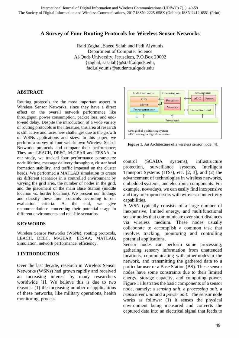
ABSTRACT
Routing protocols are the most important aspect in
Wireless Sensor Networks, since they have a direct
effect on the overall network performance like
throughput, power consumption, packet loss, and end-
to-end delay. Despite the introduction of a wide variety
of routing protocols in the literature, this area of research
is still active and faces new challenges due to the growth
of WSNs applications and sizes. In this paper, we
perform a survey of four well-known Wireless Sensor
Networks protocols and compare their performance;
They are: LEACH, DEEC, M-GEAR and EESAA. In
our study, we tracked four performance parameters:
node lifetime, message delivery throughput, cluster head
formation stability, and traffic imposed on the cluster
heads. We performed a MATLAB simulation to create
six different scenarios in a controlled environment by
varying the grid area, the number of nodes in the grid,
and the placement of the main Base Station (middle
location vs. border location). We present our findings
and classify these four protocols according to our
evaluation criteria. At the end, we give
recommendations concerning their potential usage in
different environments and real-life scenarios.
KEYWORDS
Wireless Sensor Networks (WSNs), routing protocols,
LEACH, DEEC, M-GEAR, EESAA, MATLAB,
Simulation, network performance, efficiency.
1 INTRODUCTION
Over the last decade, research in Wireless Sensor
Networks (WSNs) had grown rapidly and received
an increasing interest by many researchers
worldwide [1]. We believe this is due to two
reasons: (1) the increasing number of applications
of these networks, like military operations, health
monitoring, process
control (SCADA systems), infrastructure
protection, surveillance systems, Intelligent
Transport Systems (ITSs), etc. [2, 3], and (2) the
advancement of technologies in wireless networks,
embedded systems, and electronic components. For
example, nowadays, we can easily find inexpensive
and tiny microprocessors with wireless connectivity
capabilities.
A WSN typically consists of a large number of
inexpensive, limited energy, and multifunctional
sensor nodes that communicate over short distances
via wireless medium. These nodes usually
collaborate to accomplish a common task that
involves tracking, monitoring and controlling
potential applications.
Sensor nodes can perform some processing,
gathering sensory information from unattended
locations, communicating with other nodes in the
network, and transmitting the gathered data to a
particular user or a Base Station (BS). These sensor
nodes have some constraints due to their limited
energy, storage capacity, and computing power.
Figure 1 illustrates the basic components of a sensor
node, namely: a sensing unit, a processing unit, a
transceiver unit and a power unit. The sensor node
works as follows: (1) it senses the physical
environment being measured and converts the
captured data into an electrical signal that feeds to
A Survey of Four Routing Protocols for Wireless Sensor Networks
Raid Zaghal, Saeed Salah and Fadi Alyounis
Department of Computer Science
Al-Quds University, Jerusalem, P.O.Box 20002
{zaghal, sasalah}@staff.alquds.edu,
Figure 1. An Architecture of a wireless sensor node [4].
International Journal of Digital Information and Wireless Communications (IJDIWC) 7(1): 49-59The Society of Digital Information and Wireless Communications, 2017 ISSN: 2225-658X (Online); ISSN 2412-6551 (Print)
49
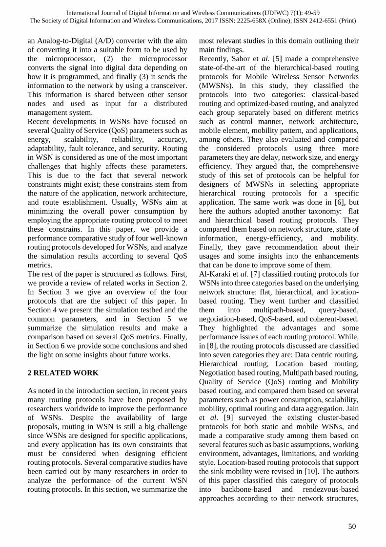
an Analog-to-Digital (A/D) converter with the aim
of converting it into a suitable form to be used by
the microprocessor, (2) the microprocessor
converts the signal into digital data depending on
how it is programmed, and finally (3) it sends the
information to the network by using a transceiver.
This information is shared between other sensor
nodes and used as input for a distributed
management system.
Recent developments in WSNs have focused on
several Quality of Service (QoS) parameters such as
energy, scalability, reliability, accuracy,
adaptability, fault tolerance, and security. Routing
in WSN is considered as one of the most important
challenges that highly affects these parameters.
This is due to the fact that several network
constraints might exist; these constrains stem from
the nature of the application, network architecture,
and route establishment. Usually, WSNs aim at
minimizing the overall power consumption by
employing the appropriate routing protocol to meet
these constrains. In this paper, we provide a
performance comparative study of four well-known
routing protocols developed for WSNs, and analyze
the simulation results according to several QoS
metrics.
The rest of the paper is structured as follows. First,
we provide a review of related works in Section 2.
In Section 3 we give an overview of the four
protocols that are the subject of this paper. In
Section 4 we present the simulation testbed and the
common parameters, and in Section 5 we
summarize the simulation results and make a
comparison based on several QoS metrics. Finally,
in Section 6 we provide some conclusions and shed
the light on some insights about future works.
2 RELATED WORK
As noted in the introduction section, in recent years
many routing protocols have been proposed by
researchers worldwide to improve the performance
of WSNs. Despite the availability of large
proposals, routing in WSN is still a big challenge
since WSNs are designed for specific applications,
and every application has its own constraints that
must be considered when designing efficient
routing protocols. Several comparative studies have
been carried out by many researchers in order to
analyze the performance of the current WSN
routing protocols. In this section, we summarize the
most relevant studies in this domain outlining their
main findings.
Recently, Sabor et al. [5] made a comprehensive
state-of-the-art of the hierarchical-based routing
protocols for Mobile Wireless Sensor Networks
(MWSNs). In this study, they classified the
protocols into two categories: classical-based
routing and optimized-based routing, and analyzed
each group separately based on different metrics
such as control manner, network architecture,
mobile element, mobility pattern, and applications,
among others. They also evaluated and compared
the considered protocols using three more
parameters they are delay, network size, and energy
efficiency. They argued that, the comprehensive
study of this set of protocols can be helpful for
designers of MWSNs in selecting appropriate
hierarchical routing protocols for a specific
application. The same work was done in [6], but
here the authors adopted another taxonomy: flat
and hierarchical based routing protocols. They
compared them based on network structure, state of
information, energy-efficiency, and mobility.
Finally, they gave recommendation about their
usages and some insights into the enhancements
that can be done to improve some of them.
Al-Karaki et al. [7] classified routing protocols for
WSNs into three categories based on the underlying
network structure: flat, hierarchical, and location-
based routing. They went further and classified
them into multipath-based, query-based,
negotiation-based, QoS-based, and coherent-based.
They highlighted the advantages and some
performance issues of each routing protocol. While,
in [8], the routing protocols discussed are classified
into seven categories they are: Data centric routing,
Hierarchical routing, Location based routing,
Negotiation based routing, Multipath based routing,
Quality of Service (QoS) routing and Mobility
based routing, and compared them based on several
parameters such as power consumption, scalability,
mobility, optimal routing and data aggregation. Jain
et al. [9] surveyed the existing cluster-based
protocols for both static and mobile WSNs, and
made a comparative study among them based on
several features such as basic assumptions, working
environment, advantages, limitations, and working
style. Location-based routing protocols that support
the sink mobility were revised in [10]. The authors
of this paper classified this category of protocols
into backbone-based and rendezvous-based
approaches according to their network structures,
International Journal of Digital Information and Wireless Communications (IJDIWC) 7(1): 49-59The Society of Digital Information and Wireless Communications, 2017 ISSN: 2225-658X (Online); ISSN 2412-6551 (Print)
50

and discussed the advantages and disadvantages of
each one of them.
Daesung et al. [11] performed a performance study
for three different types of routing protocols:
LEACH, PEGASIS, and VGA using Sensoria
Simulator [12]. Power consumption and overall
network performance were used as the QoS metrics.
Based on the simulation results, the authors argued
that PEGASIS outperforms the two others, then
LEACH and finally VGA which has the worst
power consumption when the sensing range is
limited, and the best when the sensing range is
increased. Bansal et al. [13] analyzed only LEACH
and PEGASIS based on total energy consumption,
overheads, and sensors lifetime. They argued that
PEGASIS outperforms LEACH in terms of network
lifetime, communication overhead and the
percentage of node deaths. In addition, it offers an
extended lifetime of the network due to its energy
efficiency. For large networks, the early death of
nodes reduces the network stability in LEACH as
compared to PEGASIS.
Latif et al. [14] analyzed the performance of four
routing protocols: LEACH, TEEN, SEP and DEEC
based on a proposed mathematical model they
developed. For validation purposes, they performed
analytical simulations in MATLAB by choosing a
number of performance metrics: number of alive
nodes, number of dead nodes, number of packets
delivered, and number of cluster heads. The
simulation results showed that DEEC outperforms
the others by providing feasible optimal results
against a set of constraints of their suggested
mathematical model. Guangjie et al. [15] conducted
different set of experiments in MATLAB to analyze
the performance of five routing protocols:
EDFCM, MCR, EEPCA, LEACH, and SEP. The
simulation results showed that the first three
protocols are better in terms of the time of the first
node’s death and the total number of packets
successfully delivered to the BS.
The research presented in this paper differs from
these works in two main aspects: (1) we have
selected to analyze a different set of protocols,
namely: LEACH, DEEC, M-GEAR, and EESAA,
because we felt they have comparable features plus
they represent a long time span that covers a wide
spectrum of protocols, (2) we implement the four
routing protocols using MATLAB simulation
platform, but also we create six different scenarios
in a controlled environment by varying three
parameters: the grid area (50m x 50m & 100m x
100m), the number of nodes in the grid (sparse grid:
70 in the small grid vs. condensed grid: 1000 nodes
in the big grid), and the placement of the main BS
(in the middle of the grid vs. on the border of the
grid). The aim of this study is to test the behavior of
these routing protocols when applied to different
scenarios resulted from varying these parameters.
3 THE EVALUATED ROUTING
PROTOCOLS
In this section, we give a brief overview of the four
WSN protocols analyzed in this work, namely
LEACH, DEEC, M-GEAR and EESAA. For more
information, please refer to the original papers.
3.1 LEACH Protocol
The Low Energy Adaptive Cluster Hierarchy
(LEACH) is the most popular WSNs routing
protocol, which was proposed by Heinzelman et al.
[16] many years ago, with the overall aim of
reducing power consumption. LEACH works in a
completely distributed way, and does not need to
acquire global knowledge of the network. The main
functions of LEACH can be grouped into two
phases: (1) in the setup phase several tasks are
performed related to the organizing of the network
into clusters, i.e., LEACH is based on the concept
of a hierarchical clustering, it divides the entire
network into several clusters and assigns one node
for each to be the Cluster Head (CH), CH
advertisement, and creating transmission schedule
for the entire network, and (2) a steady-state phase
that consists of data aggregation (or fusion),
compression, and transmission to the BS. LEACH
reduces energy consumption by (1) minimizing the
communication cost between sensor nodes and their
CHs, and (2) shutting down non-CH nodes as much
as possible. A CH is responsible for data collection
from the entire sensor nodes belonging to the cluster
under its control, and then it makes the necessary
processing tasks on the data before sending it to the
BS. LEACH uses a single-hop routing where each
node can directly transmit to the CH and the BS.
Therefore, it is not efficient in large networks.
Furthermore, the concept of assigning clustering
dynamically brings additional overhead such as CH
changes and advertisements, which can minimize
the gain in energy consumption. While LEACH
helps the sensor nodes within their clusters to
diminish their energy slowly, the CHs consume a
larger amount of energy when they are located at
International Journal of Digital Information and Wireless Communications (IJDIWC) 7(1): 49-59The Society of Digital Information and Wireless Communications, 2017 ISSN: 2225-658X (Online); ISSN 2412-6551 (Print)
51

the farthest point from the BS. Also, LEACH
clustering terminates in a finite number of
iterations, but does not guarantee a good CH
distribution and assumes uniform energy
consumption for CHs, i.e., it adapts a randomized
rotating mechanism of high-energy CH position
rather than making a selection in a static manner, to
give an equal chance to all sensor nodes to become
CHs.
3.2 DEEC Protocol
Distributed Energy-Efficient Clustering (DEEC)
protocol [17], is an adaptive clustering protocol
used in heterogeneous wireless sensor networks. It
assumes that in a WSN there are several types of
nodes of different initial energy levels, e.g., a WSN
with three types of nodes of initial energy levels is
a three-level heterogeneous network. In DEEC,
every sensor node independently elects itself as a
CH, and the probability for a node to be a CH is
calculated based on two parameters: (1) the ratio
between the residual energy of the node, and (2) the
average energy of the entire network. Therefore, a
node with high initial energy and residual energy
acquires more chances to become a CH. To control
the energy consumption of sensor nodes by means
of adaptive approach, DEEC uses the average
energy of the network as the reference energy.
Thus, DEEC does not require any global knowledge
of energy at every election round. Unlike LEACH,
DEEC can perform better in multi-level
heterogeneous WSNs.
3.3 M-GEAR Protocol
Gateway-Based Energy-Aware Multi-Hop routing
protocol for WSNs (M-GEAR) [18] uses a BS and
a gateway node. It divides the nodes into four
regions. The operation of the protocol consists of
five phases, in its initial phase the BS broadcast a
HELLO packet, and all nodes in the network replay
indicating their locations. Then, the BS can build
the node’s data table by saving each node’s id,
location, distance from the BS and gateway node
and residual node energy. In the second phase
(setup), the protocol divides the network into four
regions, the first one for nodes near the BS (nodes
in this region can send data directly to the BS), the
second region for nodes near the gateway node
(nodes in this region can send their data to the
gateway node which in turn aggregates the data and
forwards it to the BS). The rest of the nodes in the
network are grouped into two regions and nodes
within each region are further grouped into clusters.
The first two regions are referred to as non-
clustered regions, while the last two regions are
referred to as clustered regions. In the third phase
(CH selection) cluster heads are selected in the two
clustered regions, for that purpose, the protocol uses
the LEACH cluster head selection approach. After
the selection of CHs, each CH creates a TDMA-
based time-slots for its member nodes, so that each
node can transmit its data in its time-slot and switch
to an idle mode for the rest of the time, this phase is
called (scheduling phase). The final phase of the
protocol is operation (the steady-state phase), in
which all sensor nodes transmit their sensed data to
its cluster heads, which in turn receive and
aggregate the data of all its member nodes and send
it to the gateway node. After collecting the data
from all CHs, the gateway node aggregates the data
and sends it to the BS.
3.4 EESAA Protocol
Energy Efficient Sleep Awake Aware intelligent
sensor network routing protocol (EESAA) [19] uses
the concept of pairing and equipping the nodes with
Global Positioning System (GPS) capabilities. In
addition to the enhanced cluster head selection
technique, the protocol was designed to improve
network stability period and prolong the network
lifetime.
Sensor nodes use their GPS to calculate their own
locations and send them to the BS, where in the first
round; cluster head selection takes place using
LEACH CH selection technique. When BS receives
the nodes’ location information, it groups the nodes
into pairs (create couples) based on the minimum
distance from each other in their intra-cluster
transmission range, and also they should belong to
the same application type. Then it broadcasts this
“pairing” information to all nodes in the network for
each node to become aware its coupled node.
During a single communication interval, paired
nodes switch between awake and sleep modes. In
any given pair, at first the node closer to the BS
switch into awake mode (active mode) and is
responsible to collect data from its surroundings
and send it to the CH, while its coupled node
remains in sleep mode during this period. In the
next round, nodes in active mode switch into sleep
mode while its couple becomes awake, and so forth.
International Journal of Digital Information and Wireless Communications (IJDIWC) 7(1): 49-59The Society of Digital Information and Wireless Communications, 2017 ISSN: 2225-658X (Online); ISSN 2412-6551 (Print)
52

Unpaired nodes remain in active mode in all the
rounds until they die.
The selection of CHs after the first round depends
on remaining energy of active nodes only, so in the
start of each round nodes transmit information
about their energy to CH, which in turn calculates
the energy of every node in its cluster and distance
from each node and select CH for the next round. In
this regard, the selected CH broadcast an
advertisement message that can be heard by every
awake node to select their CH according to the
received signal strength indication of those
advertisements. Finally, nodes in active mode are
the only nodes allowed to transmit their sensed data
during their TDMA-slots while nodes in sleep mode
turn their transceivers off to save energy.
4 SIMULATION TESTBED
As mentioned earlier, we have used MATLAB to
run our simulations. MATLAB is an ideal choice
for WSN simulations since it gives accurate results
and includes built-in capabilities. For each
simulation scenario, we designed a network with a
predefined area and then distributed a given number
of nodes randomly within that area. Each one of the
four protocols has been simulated with 6 different
scenarios (as shown in Table 2), but in all of these
scenarios we used common fixed radio parameters.
Also, each node was considered dead when its
internal energy approaches zero. To simulate
message exchanges between nodes we used a fixed
message size of 4000 bit, and finally, it is worth
mentioning that we assumed the network to be free
of collisions. Table 1 lists the network parameters
used in the testbed scenarios.
The four WSN routing protocols surveyed in this
study are already built-in MATLAB, which we
believe is a very good thing since it enables us to
get reliable and consistent results. We designed the
testbed to simulate six scenarios for of each one of
the four protocol to study the impact of changing
the sink node position, the impact of having
different network sizes and densities, and the
number of nodes and their distributions. In the
following subsections, a summary about the setup
variables on each scenario will be listed, then we
provide the main differences between the four
protocols LEACH, DEEC, M-GEAR and EESAA
using four parameters: (i) the number of the dead
nodes per round, (ii) the number of packets
successfully received by the BS, (iii) the number of
cluster heads per round, and finally (iv) the number
of packets that went through the cluster heads. Next,
we make a comparative study of their performance
in six scenarios in order to study the impact of
changing the position of the sink node, network
size, and nodes distributions.
Table 1. Network simulation parameters.
Parameter Value Description
Eelec 50 nj/bits power needed to run the
transmitter or receiver
circuitry
Efs 10 pj/bit/m2 % Transmit Amplifier
type
EDA 50 nj/bit/packet Data Aggregation
Energy
E0 0.5 J Initial Energy
Number of
rounds
5000 --
Emp 0.013pj/bit/m4 % Another Transmit
Amplifier type
5 SIMULATION RESULTS AND DISCUSSION
As previously mentioned, in the first two scenarios
we built a small-area scattered network of 70 nodes
dispersed randomly in 50m * 50m simulation area
with a BS located at the center and the border
respectively. In the third and fourth scenarios, we
built a dense network of 500 nodes distributed
randomly in 100m * 100m area with BS located at
the center and the border of the area respectively,
and finally in the fifth and sixth scenarios, we built
a highly- dense network of 1000 nodes distributed
randomly in 100m * 100m area with BS located at
the center and the border of the area respectively.
Table 2 summarizes the characteristics of these six
simulation scenarios.
Table 2. The six simulated scenarios.
Scenario Num. of
nodes Area
BS
location Property
S1 70 50m x 50m Center Sparse
S2 70 50m x 50m Border Sparse
S3 500 100m x 100m Center Dense
S4 500 100m x 100m Border Dense
S5 1000 100m x 100m Center Hi-Dense
S6 1000 100m x 100m Border Hi-Dense
International Journal of Digital Information and Wireless Communications (IJDIWC) 7(1): 49-59The Society of Digital Information and Wireless Communications, 2017 ISSN: 2225-658X (Online); ISSN 2412-6551 (Print)
53
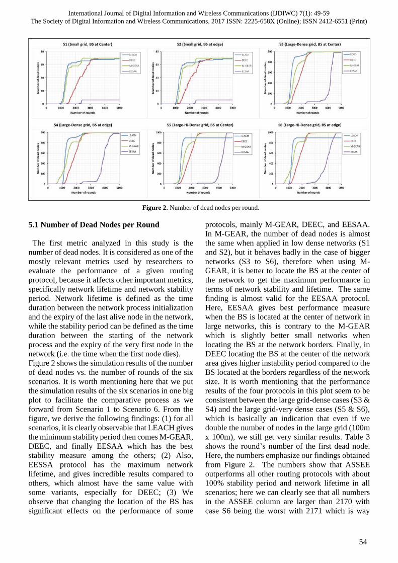
5.1 Number of Dead Nodes per Round
The first metric analyzed in this study is the
number of dead nodes. It is considered as one of the
mostly relevant metrics used by researchers to
evaluate the performance of a given routing
protocol, because it affects other important metrics,
specifically network lifetime and network stability
period. Network lifetime is defined as the time
duration between the network process initialization
and the expiry of the last alive node in the network,
while the stability period can be defined as the time
duration between the starting of the network
process and the expiry of the very first node in the
network (i.e. the time when the first node dies).
Figure 2 shows the simulation results of the number
of dead nodes vs. the number of rounds of the six
scenarios. It is worth mentioning here that we put
the simulation results of the six scenarios in one big
plot to facilitate the comparative process as we
forward from Scenario 1 to Scenario 6. From the
figure, we derive the following findings: (1) for all
scenarios, it is clearly observable that LEACH gives
the minimum stability period then comes M-GEAR,
DEEC, and finally EESAA which has the best
stability measure among the others; (2) Also,
EESSA protocol has the maximum network
lifetime, and gives incredible results compared to
others, which almost have the same value with
some variants, especially for DEEC; (3) We
observe that changing the location of the BS has
significant effects on the performance of some
protocols, mainly M-GEAR, DEEC, and EESAA.
In M-GEAR, the number of dead nodes is almost
the same when applied in low dense networks (S1
and S2), but it behaves badly in the case of bigger
networks (S3 to S6), therefore when using M-
GEAR, it is better to locate the BS at the center of
the network to get the maximum performance in
terms of network stability and lifetime. The same
finding is almost valid for the EESAA protocol.
Here, EESAA gives best performance measure
when the BS is located at the center of network in
large networks, this is contrary to the M-GEAR
which is slightly better small networks when
locating the BS at the network borders. Finally, in
DEEC locating the BS at the center of the network
area gives higher instability period compared to the
BS located at the borders regardless of the network
size. It is worth mentioning that the performance
results of the four protocols in this plot seem to be
consistent between the large grid-dense cases (S3 &
S4) and the large grid-very dense cases (S5 & S6),
which is basically an indication that even if we
double the number of nodes in the large grid (100m
x 100m), we still get very similar results. Table 3
shows the round’s number of the first dead node.
Here, the numbers emphasize our findings obtained
from Figure 2. The numbers show that ASSEE
outperforms all other routing protocols with about
100% stability period and network lifetime in all
scenarios; here we can clearly see that all numbers
in the ASSEE column are larger than 2170 with
case S6 being the worst with 2171 which is way
Figure 2. Number of dead nodes per round.
International Journal of Digital Information and Wireless Communications (IJDIWC) 7(1): 49-59The Society of Digital Information and Wireless Communications, 2017 ISSN: 2225-658X (Online); ISSN 2412-6551 (Print)
54
better than the other three. Then comes DEEC,
LEACH, and M-GEAR, and in that order; DEEC in
the range 930 (worst performance in S4) and 1390
(best performance in S1), LEACH in the range 892
(worst performance in S6) and 984 (best
performance in S3 & S4), and finally M-GEAR in
the range 521 (worst performance in S6) and 1070
(best performance in S1). This is evidence that
DEEC and M-GEAR are badly affected by the
number of nodes in the grid. Furthermore, M-
GEAR has almost the same performance measure
as DEEC for the first two scenarios, while it gives
the minimum performance results in the large and
dense grids.
Table 3. Round’s number of the first dead node.
Scenario LEACH DEEC M-GEAR EESAA
S1 912 1391 1070 2236
S2 978 1113 1053 2283
S3 984 994 630 2233
S4 983 934 526 2182
S5 966 1042 597 2336
S6 892 1018 521 2171
5.2 Packets to the Base Station
In this section, we study another performance
metric which is the number of data packets
successfully received by the BS. This metric gives
good measures about the reliability of the network,
i.e., it presents a good indicator whether the routing
protocol is doing its job properly or not. Figure 3
shows the simulation results of the six scenarios.
Several findings are extracted as follows: (1) in the
first two scenarios (S1, S2), DEEC outperforms the
others in the number of packets successfully
delivered to the BS, then comes M-GEAR, EESAA,
and finally the LEACH which has the minimum
number of packets received by the BS. Whereas, in
scenarios S3 and S4, EESAA outperforms all of
them, while M-GEAR gives the minimum number.
Both DEEC and LEACH are located at the middle;
(2) regarding the effect of the location of the BS, we
find that in LEACH the number of packets
delivered to the BS is almost the same whether the
BS is located at the center or at the borders of the
network, with a slightly higher number in the
former case. DEEC gives the best results of packet
delivery ratio, mainly when the BS is located at the
center. Like DEEC, M-GEAR does the best job
when the BS is located at the center. Finally, there
is a significant effect of the location of the BS on
the functioning of EESSA. Here, we observe that
EESAA gives better results when the BS is located
at the center when deployed in large networks (S3
and S4), whereas in the case of small networks (S1
and S2) its highly recommended to put the BS at the
borders to get the maximum benefits of this
protocol.
5.3 Cluster Heads Formation
Figure 3. Number of packets received by the BS.
International Journal of Digital Information and Wireless Communications (IJDIWC) 7(1): 49-59The Society of Digital Information and Wireless Communications, 2017 ISSN: 2225-658X (Online); ISSN 2412-6551 (Print)
55

The third performance metric considered in this
study is the stability of the cluster heads formation
process. This process plays an important role in the
stability of the whole network.
Unlike the aforementioned performance metrics, a
protocol having a large number of cluster heads per
round does not mean that the protocol behaves
better than of those having small ones. Here, we
perform the analytical study considering that the
cluster heads per round for a particular protocol is
much closer to the optimal situation when this
number follows a uniform
distribution within the network lifetime. Based on
this definition, Figure 4 shows the simulation
results of the four protocols. Here, we extract the
following findings: (1) in all scenarios, it’s obvious
that EESAA has the highest stability in cluster head
formation process as the number of cluster heads
created is uniformly distributed within the whole
network lifetime with an average of 4 cluster
heads/round. DEEC has low cluster formation
stability in all scenarios; in small grid networks
LEACH shows low cluster formation stability, but
in large grid networks it shows moderate stability
level. M-GEAR also has a moderate level of cluster
stability for all scenarios. (2) contrary to what is
expected, M-GEAR creates a small number of
cluster heads per round as the network becomes
larger (S3 to S6). This is due to some design issues
behind this protocol. In the setup phase of the
operation of this protocol, it divides the network
into four regions; the first one consists of nodes
which are located near the BS. Nodes in this region
can send data directly to the BS; The second region
encompasses a set of nodes that are close to the
gateway node. Nodes in this region send their data
to the gateway node, which in turn aggregates the
data and forward it to the BS; the remaining nodes
are grouped into two regions, and nodes belonging
to a group are further split into more clusters. The
first two regions are referred to as non-clustered
regions, while the last two are referred to as
clustered regions. This process explains the
behavior of M-GEAR protocol in creating fewer
cluster heads in the large grids compared to the
small ones.
5.4 Number of Packets at Cluster Heads
As the fourth and last performance metric in our
study, we will study the impact of the total number
of packets that went through the cluster heads on the
network. We can consider this parameter as an
approximation of the centralized nature of the
protocol and the overhead traffic imposed by the
protocol on the cluster-heads. Figure 5 presents the
simulation results of the four protocols. Here, we
can extract the following findings: (1) in the
small/sparse grid (S1 & S2), all protocols are
generating big and noisy traffic at the cluster heads,
while they perform better when the grid is big and
dense where we can see smoother and smaller plots,
(2) it seems that the BS location being at the center
or at the edge does not really affect this parameter.
Figure 4. Number of cluster heads.
International Journal of Digital Information and Wireless Communications (IJDIWC) 7(1): 49-59The Society of Digital Information and Wireless Communications, 2017 ISSN: 2225-658X (Online); ISSN 2412-6551 (Print)
56
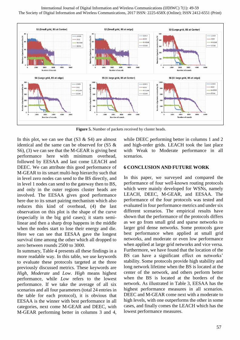
In this plot, we can see that (S3 & S4) are almost
identical and the same can be observed for (S5 &
S6), (3) we can see that the M-GEAR is giving best
performance here with minimum overhead,
followed by EESAA and last come LEACH and
DEEC. We can attribute this good performance of
M-GEAR to its smart multi-hop hierarchy such that
in level zero nodes can send to the BS directly, and
in level 1 nodes can send to the gateway then to BS,
and only in the outer regions cluster heads are
involved. The EESAA gives good performance
here due to its smart pairing mechanism which also
reduces this kind of overhead, (4) the last
observation on this plot is the shape of the curve
(especially in the big grid cases); it starts semi-
linear and then a sharp drop happens in the middle
when the nodes start to lose their energy and die.
Here we can see that EESAA gave the longest
survival time among the other which all dropped to
zero between rounds 2500 to 3000.
In summary, Table 4 presents all these findings in a
more readable way. In this table, we use keywords
to evaluate these protocols targeted at the three
previously discussed metrics. These keywords are
High, Moderate and Low. High means highest
performance, while Low refers to the lowest
performance. If we take the average of all six
scenarios and all four parameters (total 24 entries in
the table for each protocol), it is obvious that
EESAA is the winner with best performance in all
categories, next come M-GEAR and DEEC, with
M-GEAR performing better in columns 3 and 4,
while DEEC performing better in columns 1 and 2
and high-order grids. LEACH took the last place
with Weak to Moderate performance in all
scenarios.
6 CONCLUSION AND FUTURE WORK
In this paper, we surveyed and compared the
performance of four well-known routing protocols
which were mainly developed for WSNs, namely
LEACH, DEEC, M-GEAR, and EESAA. The
performance of the four protocols was tested and
evaluated in four performance metrics and under six
different scenarios. The empirical results have
shown that the performance of the protocols differs
as we go from small grid and sparse networks to
larger grid dense networks. Some protocols gave
best performance when applied at small grid
networks, and moderate or even low performance
when applied at large grid networks and vice versa.
Furthermore, we have found that the location of the
BS can have a significant effect on networks’
stability. Some protocols provide high stability and
long network lifetime when the BS is located at the
center of the network, and others perform better
when the BS is located at the borders of the
network. As illustrated in Table 3, EESAA has the
highest performance measures in all scenarios.
DEEC and M-GEAR come next with a moderate to
high levels, with one outperforms the other in some
cases, and finally comes the LEACH which has the
lowest performance measures.
Figure 5. Number of packets received by cluster heads.
International Journal of Digital Information and Wireless Communications (IJDIWC) 7(1): 49-59The Society of Digital Information and Wireless Communications, 2017 ISSN: 2225-658X (Online); ISSN 2412-6551 (Print)
57

Based on these findings, we will continue to
investigate the performance of these routing
protocols in more complicated scenarios and will
try to combine the best features in them (which led
to their good performance) specially EESAA and
DEEC, to design a new (hybrid) routing protocol
and test it as well.
REFERENCES
1. I. F. Akyildiz, Weilian Su, Y. Sankarasubramaniam and
E. Cayirci, “A survey on sensor networks,” in IEEE
Communications Magazine, vol. 40, no. 8, pp. 102-114,
Aug 2002. doi: 10.1109/MCOM.2002.1024422.
2. J. Yick, B. Mukherjee, and D. Ghosal, “Wireless sensor
network survey,” Computer Networks, vol. 52, issue 12,
pp. 2292-2330, August 2008, ISSN 1389-1286,
http://dx.doi.org/10.1016/j.comnet.2008.04.002.
3. D. Culler, D. Estrin, and M. Srivastava, “Overview of
sensor networks,” Computer Magazine,IEEE, vol. 37, no.
8, pp. 41-49, August 2004.
4. C. Y. Lin, S. Zeadally, T. S. Chen, and C. Y. Chang,
“Enabling cyber physical systems with wireless sensor
networking technologies,” International Journal of
Distributed Sensor Networks, vol. 2012, Article ID
489794, 21 pages, 2012. doi:10.1155/2012/489794
5. Nabil Sabor, Shigenobu Sasaki, Mohammed Abo-
Zahhad, and Sabah M. Ahmed, “A Comprehensive
Survey on Hierarchical-Based Routing Protocols for
Mobile Wireless Sensor Networks: Review, Taxonomy,
and Future Directions,” Wireless Communications and
Mobile Computing, vol. 2017, Article ID 2818542, 23
pages, 2017. doi:10.1155/2017/2818542.
6. G. S. Sara and D. Sridharan, “Routing in mobile wireless
sensor network: a survey,” Telecommunication Systems,
vol. 57, no. 1, pp. 51–79, 2014.
7. J. N. Al-Karaki and A. E. Kamal, “Routing techniques in
wireless sensor networks: a survey,” in IEEE Wireless
Communications, vol. 11, no. 6, pp. 6-28, Dec. 2004. doi:
10.1109/MWC.2004.1368893.
H. S. Bazzi, A. M. Haidar, and A. Bilal, “Classification
of routing protocols in wireless sensor
network,” Computer Vision and Image Analysis
Applications (ICCVIA), 2015 International Conf. on,
IEEE, 2015.
8. M. Patil and R. C. Biradar, “A survey on routing
protocols in wireless sensor networks,” 2012 18th IEEE
International Conf. on Networks (ICON), Singapore,
2012, pp. 86-91.
doi: 10.1109/ICON.2012.6506539.
9. S. R. Jain and N. V. Thakur, “Overview of cluster based
routing protocols in static and mobile wireless sensor
networks,” in Information Systems Design and Intelligent
Applications: Proceedings of Second International
Conference INDIA 2015, Volume 1, pp. 619–626,
Springer India, New Delhi, India, 2015.
10. K. Daesung, K. Dongkyun, P. Hyeon, and Y. Seung-mok,
“Performance evaluation of routing protocols for wireless
sensor networks in military scenarios,” 2011 Third
International Conf. on Ubiquitous and Future Networks
(ICUFN), Dalian, 2011, pp. 101-106.
doi: 10.1109/ICUFN.2011.5949143.J. Wang, X. Yang, Z.
Table 4. Summary results.
Protocol Scenario Network Stability Packets Transfer
Rate
Cluster Formation
Stability
Packets to CH
Overhead
LEACH S1 Moderate Low Low Low
S2 Moderate Low Low Low
S3 Moderate Moderate Moderate Low
S4 Moderate Moderate Moderate Low
S5 Low Low Low Low
S6 Low Low Low Low
DEEC S1 Moderate High Moderate Moderate
S2 Moderate High Moderate Moderate
S3 Moderate High Low Low
S4 Moderate Moderate Low Low
S5 Moderate Moderate Low Low
S6 Moderate Moderate Low Low
M-GEAR S1 Moderate Moderate High High
S2 Moderate High Moderate High
S3 Low Low Moderate High
S4 Low Low Moderate High
S5 Moderate High Moderate High
S6 Moderate High Moderate High
EESAA S1 High Low High High
S2 High Moderate High High
S3 High High High High
S4 High High High High
S5 High Moderate High High
S6 High Moderate High High
International Journal of Digital Information and Wireless Communications (IJDIWC) 7(1): 49-59The Society of Digital Information and Wireless Communications, 2017 ISSN: 2225-658X (Online); ISSN 2412-6551 (Print)
58

Zhang, B. Li, and J.-U. Kim, “A survey about routing
protocols with mobile sink for wireless sensor network,”
International Journal of Future Generation
Communication and Networking, vol. 7, no. 5, pp. 221–
228, 2014.
11. J. N. Al-Karaki, and G. A. Al-Mashaqbeh, “SENSORIA:
a new simulation platform for wireless sensor networks,”
International Conf. on Sensor Technologies and
Applications, pp: 424 - 429. 2007.
12. B. Parul, P. Kundu, and P. Kaur, “Comparison of LEACH
and PEGASIS hierarchical routing protocols in wireless
sensor networks,” International Journal on Recent Trends
in Engineering & Technology , 11.1 (2014): 139.
13. K. Latif, M. Jaffar, N. Javaid, M. N. Saqib, U. Qasim, and
Z. A. Khan, “Performance analysis of hierarchical routing
protocols in wireless sensor networks,” In Proceedings
of the 2012 Seventh International Conf. on Broadband,
Wireless Computing, Communication and
Applications (BWCCA '12). IEEE Computer Society,
Washington, DC, USA, pp. 620-625.
DOI=http://dx.doi.org/10.1109/BWCCA.2012.108,
2012.
14. G. Han, X. Jiang, A. Qian, J. J. P. C. Rodrigues, and L.
Cheng, “A comparative study of routing protocols of
heterogeneous wireless sensor networks,” The Scientific
World Journal, vol. 2014, Article ID 415415, 11 pages,
2014. doi:10.1155/2014/41541.
15. W. R. Heinzelman, A. Chandrakasan and H.
Balakrishnan, “Energy-efficient communication protocol
for wireless microsensor networks,” System Sciences,
2000. Proceedings of the 33rd Annual Hawaii
International Conf. on, 2000, pp.10-pp, vol.2, doi:
10.1109/HICSS.2000.926982.
16. Q. Nadeem, M. B. Rasheed, N. Javaid, Z. A. Khan, Y.
Maqsood and A. Din, "M-GEAR: Gateway-Based
Energy-Aware Multi-hop Routing Protocol for WSNs,"
Broadband and Wireless Computing, Communication
and Applications (BWCCA), 2013 Eighth International
Conference on, Compiegne, 2013, pp. 164-169, doi:
10.1109/BWCCA.2013.35.
17. L. Qing, Q. Zhu, and M. Wang, “Design of a distributed
energy-efficient clustering algorithm for heterogeneous
wireless sensor networks,” Comput. Commun. 29, 12
(August 2006),2230-2237. DOI =
http://dx.doi.org/10.1016/ j.comcom.2006.02.017.
18. Shah, T., Javaid, N., & Qureshi, T. N., “Energy efficient
sleep awake aware (EESAA) intelligent sensor network
routing protocol,” In 15th IEEE International Multitopic
Conference (INMIC), pp. 317-322, 2012.
International Journal of Digital Information and Wireless Communications (IJDIWC) 7(1): 49-59The Society of Digital Information and Wireless Communications, 2017 ISSN: 2225-658X (Online); ISSN 2412-6551 (Print)
59

The International Journal of Digital Information and Wireless Communications aims to provide a forum for scientists, engineers, and practitioners to present their latest research results, ideas, developments and applications in the field of computer architectures, information technology, and mobile technologies. The IJDIWC publishes issues four (4) times a year and accepts three types of papers as follows:
1. Research papers: that are presenting and discussing the latest, and the most profound research results in the scope of IJDIWC. Papers should describe new contributions in the scope of IJDIWC and support claims of novelty with citations to the relevant literature.
2. Technical papers: that are establishing meaningful forum between practitioners and researchers with useful solutions in various fields of digital security and forensics. It includes all kinds of practical applications, which covers principles, projects, missions, techniques, tools, methods, processes etc.
3. Review papers: that are critically analyzing past and current research trends in the field.
Manuscripts submitted to IJDIWC should not be previously published or be under review by any other publication. Original unpublished manuscripts are solicited in the following areas including but not limited to:
Information Technology Strategies
Information Technology Infrastructure
Information Technology Human Resources
System Development and Implementation
Digital Communications
Technology Developments
Technology Futures
National Policies and Standards
Antenna Systems and Design
Channel Modeling and Propagation
Coding for Wireless Systems
Multiuser and Multiple Access Schemes
Optical Wireless Communications
Resource Allocation over Wireless Networks
Security; Authentication and Cryptography for Wireless Networks
Signal Processing Techniques and Tools
Software and Cognitive Radio
Wireless Traffic and Routing Ad-hoc Networks
Wireless System Architectures and Applications
International Journal of DIGITAL INFORMATION AND WIRELESS COMMUNICATIONS