a genetic algorithm application for mtf analysis · a genetic algorithm application for mtf...
TRANSCRIPT

A Genetic Algorithm Application for MTF Analysis
Lydia M. Knurek
Advisers: Dr. Jonathan S. Arney and Dr. Peter G. Andersen
Center for Imaging Science
Rochester Institute of Technology
14 May 2004

2
Table of Contents
1. Abstract ………………………………..………... 3
2. Problem Statement …………………………….. 3-5
3. Technical Background ……….......…………….. 5-7
3.1. MTF Analysis 3.2. Genetic Algorithms
4. Development of the Algorithm ….…………….. 7-13
4.1. The Edges to be Analyzed 4.2. The Initial MTF Population 4.3. The Figure of Merit 4.4. The Breeding Process
5. Results ....……………………………..………… 13-25
5.1. Initial Genetic Algorithm 5.2. Constraints Applied to the Algorithm 5.3. Calculating the MTF from the GA Edge 5.4. Analysis of Noisy Edges
6. Conclusion …….……………………….….….... 25-26 7. Appendix ……………………………………..... 27-29
7.1. Computational Details 7.2. Source Code
8. References ………………………………….….. 30

3
1 Abstract
The modulation transfer function (MTF) is an important characteristic of an imaging system because it portrays how much modulation at a specific frequency is maintained by the imaging process. Noise in the resulting image data from the system makes it difficult to estimate the true system MTF. The purpose of this project was to use a genetic algorithm, in the frequency domain, monitored by the RMS deviation in the spatial domain, to estimate the MTF. The preliminary MTF data created by the algorithm generates edge data with noise that is represented by the overall slope of the data. The noise is eliminated by subtracting out the sloped line. This produces an edge with noise filtered out, without altering the edge itself. The final, smoothed edge is then used in a traditional MTF analysis to provide a noiseless estimate of the true system MTF.
2 Problem Statement
Past research1 and a quick example, (Figure 1), show that a noisy edge gives a poor estimate of the true system MTF when a traditional MTF analysis is applied.
Figure 1A: Noiseless Edge and Noisy Edge Example
1 J.S. Arney, J. Chauvin, J. Nauman, and P.G. Anderson
4
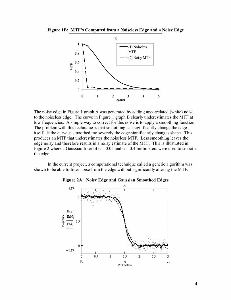
Figure 1B: MTF’s Computed from a Noiseless Edge and a Noisy Edge
B
0
0.2
0.4
0.6
0.8
1
0 1 2 3 4 5cy/mm
MT
F
(1) NoiselessMTF(2) Noisy MTF
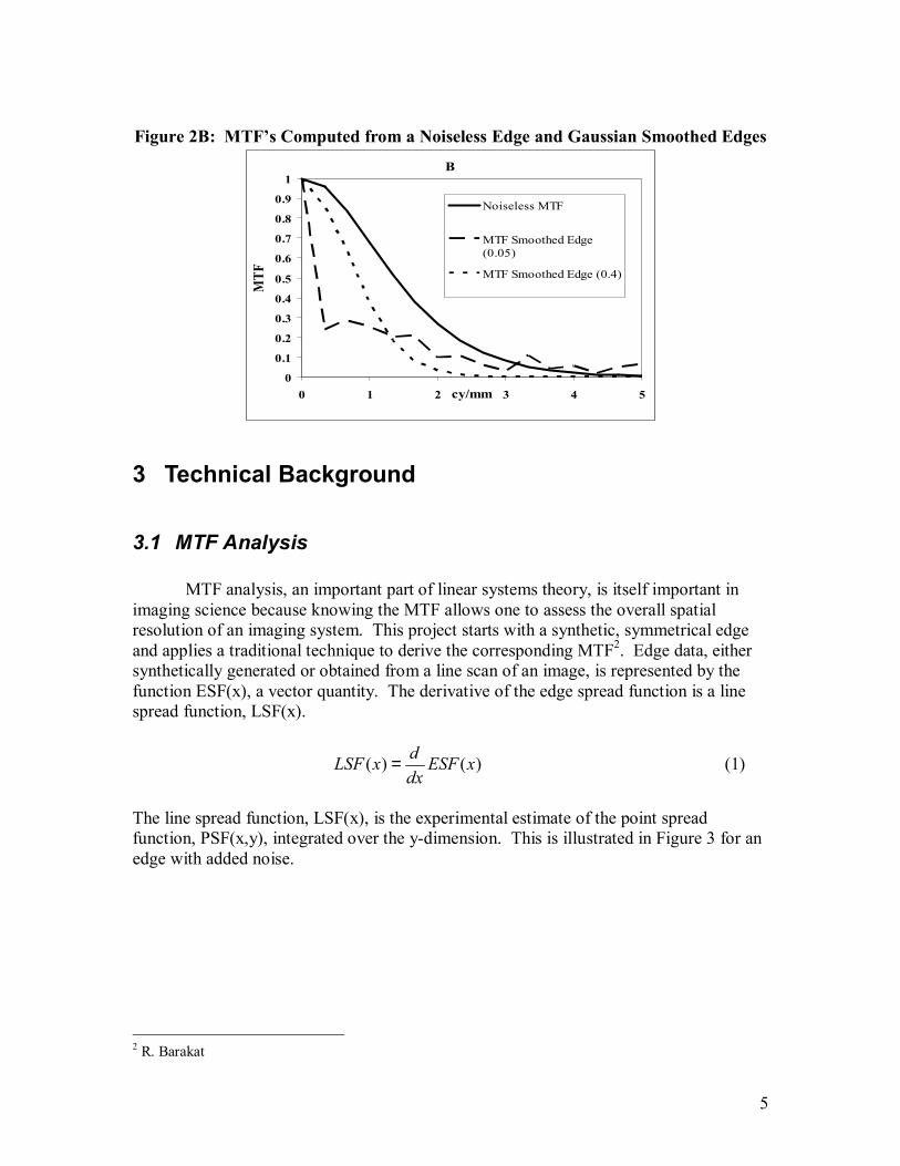
The noisy edge in Figure 1 graph A was generated by adding uncorrelated (white) noise to the noiseless edge. The curve in Figure 1 graph B clearly underestimates the MTF at low frequencies. A simple way to correct for this noise is to apply a smoothing function. The problem with this technique is that smoothing can significantly change the edge itself. If the curve is smoothed too severely the edge significantly changes shape. This produces an MTF that underestimates the noiseless MTF. Less smoothing leaves the edge noisy and therefore results in a noisy estimate of the MTF. This is illustrated in Figure 2 where a Gaussian filter of σ = 0.05 and σ = 0.4 millimeters were used to smooth the edge. In the current project, a computational technique called a genetic algorithm was shown to be able to filter noise from the edge without significantly altering the MTF.
Figure 2A: Noisy Edge and Gaussian Smoothed Edges
5
Figure 2B: MTF’s Computed from a Noiseless Edge and Gaussian Smoothed Edges
B
0
0.1
0.2
0.3
0.4
0.5
0.6
0.7
0.8
0.9
1
0 1 2 3 4 5cy/mm
MTF
Noiseless MTF
MTF Smoothed Edge(0.05)
MTF Smoothed Edge (0.4)
3 Technical Background
3.1 MTF Analysis MTF analysis, an important part of linear systems theory, is itself important in imaging science because knowing the MTF allows one to assess the overall spatial resolution of an imaging system. This project starts with a synthetic, symmetrical edge and applies a traditional technique to derive the corresponding MTF2. Edge data, either synthetically generated or obtained from a line scan of an image, is represented by the function ESF(x), a vector quantity. The derivative of the edge spread function is a line spread function, LSF(x).
)()( xESFdxdxLSF = (1)
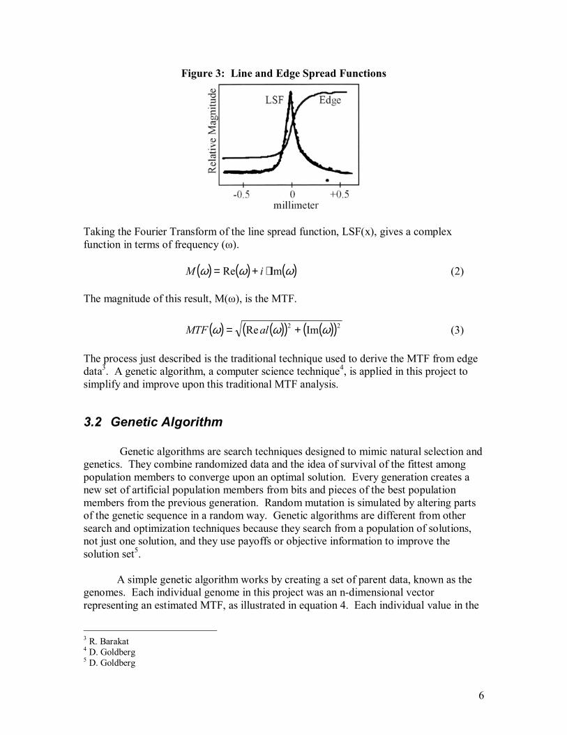
The line spread function, LSF(x), is the experimental estimate of the point spread function, PSF(x,y), integrated over the y-dimension. This is illustrated in Figure 3 for an edge with added noise.
2 R. Barakat
6
Figure 3: Line and Edge Spread Functions
Taking the Fourier Transform of the line spread function, LSF(x), gives a complex function in terms of frequency (ω).
( ) ( ) ( )ωωω ImRe ⋅+= iM (2)
The magnitude of this result, M(ω), is the MTF.
( ) ( )( ) ( )( )22 ImRe ωωω += alMTF (3) The process just described is the traditional technique used to derive the MTF from edge data3. A genetic algorithm, a computer science technique4, is applied in this project to simplify and improve upon this traditional MTF analysis.
3.2 Genetic Algorithm Genetic algorithms are search techniques designed to mimic natural selection and genetics. They combine randomized data and the idea of survival of the fittest among population members to converge upon an optimal solution. Every generation creates a new set of artificial population members from bits and pieces of the best population members from the previous generation. Random mutation is simulated by altering parts of the genetic sequence in a random way. Genetic algorithms are different from other search and optimization techniques because they search from a population of solutions, not just one solution, and they use payoffs or objective information to improve the solution set5. A simple genetic algorithm works by creating a set of parent data, known as the genomes. Each individual genome in this project was an n-dimensional vector representing an estimated MTF, as illustrated in equation 4. Each individual value in the
3 R. Barakat 4 D. Goldberg 5 D. Goldberg

7
genome is referred to as a gene. The population consisted of m individuals, MTF1 to MTFm. Each ai,j is a gene for individual i at spatial frequency j. MTF1(ξ) = [a1,1, a1,2, a1,3……..a1,16, a1,17, a1,n] MTF2(ξ) = [a2,1, a2,2, a1,3……..a2,16, a2,17, a2,n] . (4) . MTFm(ξ) = [am,1, am,2, am,3……..am,16, am,17, am,n]
A fitness statistic is computed for each genome (MTF vector) by comparing it to a known standard. The standard in the current project will be discussed later. Typically the RMS deviation between each genome and the standard is calculated for the fitness statistic. This becomes the Figure of Merit (FOM) for the genomes. The genomes are then sorted based on this FOM.
MTF1(ξ) = [a1,1, a1,2, a1,3……..a1,16, a1,17, a1,n] FOM1 MTF2(ξ) = [a2,1, a2,2, a1,3……..a2,16, a2,17, a2,n] FOM2 . (5) . MTFm(ξ) = [am,1, am,2, am,3……..am,16, am,17, am,n] FOMm
The genomes become a set of parents, and the best parents, based on the fitness,
are allowed to breed. Breeding is simulated by replacing the worst members of the population. Breeding can consist of replacing the worst genomes with exact copies or random combinations of other genomes. A random mutation can also be included in the process. This is done by adding a small random number to some randomly selected genes. After all of the breeding and mutation is complete, a fitness statistic is calculated again and the process repeats for a number of cycles. Typically, many thousands of cycles are required to evolve optimal genome solutions.
The fitness statistic is monitored and when it reaches a desired level, or ceases to
change, the loops end and the optimal solution has been found. There are many different breeding techniques, mutation techniques, and constraints that can be placed on the algorithm. Testing different techniques is necessary in order to find the optimal solution and to improve the rate at which the optimal solutions are approached.
4 Development of the Algorithm
4.1 The Edges to be Analyzed
The initial intent of this genetic algorithm was to derive the MTF from input edge spread data. The algorithm, written in MATLAB, first reads in the edge spread data in question. For this research, synthetically generated edges were used. This data was created using the equation shown below, with x in millimeters and γ, a unit less constant equal to the slope, dy/dx, at y = 0.5.

8
( ) ( )[ ]5.14exp11
−−+=
xxy
γ (6)
In this project, a value of γ = 3 was used. One noiseless edge was generated using equation 6. This edge was a vector of 640 values, aj, corresponding to 640 locations of 0 ≤ xi,j ≤ 1.5 mm. A number of edges were created with varying amounts of noise. Noisy edges were created by adding random noise to the edge generated with Equation 6. Each edge had a pre-determined standard deviation and a mean value of zero. Seven levels of noise were created and each level had an increasingly larger standard deviation. For example, noise level 1 had a standard deviation of 0.01σ and noise level 20 had a standard deviation of 0.2σ.
4.2 The Initial MTF Population
A set of m = 50 genomes was generated with n = 100 genes in each. The data set represents a population of MTFs. Each was constrained so that the first and last values were equal to1 to reflect the symmetry of the MTF. The rest of the values were created with a random number generator and varied between zero and one. To simulate the symmetry of the MTF a set of 50 genes was first created for each of the 50 genomes. These genes were then mirrored to create the second half of the MTF population matrix. This is illustrated in equation 7 where each ai,j is a random number between 0 and 1.
50,5049,502,50
50,4949,492,49
50,249,22,2
50,149,12,1
...1
...1......
...1
...150
aaaaaa
aaaaaa
genomesofSetInitial
1...1.........1...1...
...1
...1......
...1
...150
2,5049,5050,50
2,4949,4950,49
2,249,250,2
2,149,150,1
50,5049,502,50
50,4949,492,49
50,249,22,2
50,149,12,1
aaaaaa
aaaaaa
aaaaaa
aaaaaa
genomesofSetMirrored
(7)

9
4.3 The Figure of Merit
At this point the loop was started. Each genome created was first backed through the MTF analysis technique described above to obtain edge data.
To start the inverse of the MTF analysis, the magnitude of the inverse Fourier transform was computed for every genome. The zero location was then shifted to the center to create a line spread function. One example of a line spread function computed from a genome MTF is shown in Figure 4.
{ } genomesofnumberiwhereMTFFFTLSF ii K11 == − (8)
Figure 4: Line Spread Function Compute from Genome MTF
Each line spread function, LSFi, was then integrated (cumulatively summed) to
get a preliminary estimate of the edge spread function, y(x).
genesofnumberjwhereLSFyj
xii K1
1==∑
= (9)
The graph in Figure 5 illustrates that the result of this integration is not a simple edge; it has a linear trend due to the cumulative sum. IxSy += * (10)

10
Figure 5: Integrated Line Spread Function
The equation of this linear trend was found from the first 25 percent of the data
points using a simple linear regression. For the ith genome with 100 genes the slope was found between points yi,25 and yi,1.
125
1,25,
−−
= iii
yyS (11)
The intercept was found using the slope and the point (i,25). 25,*25 iii ySI +−= (12) This equation was then subtracted from each point. ( )ijiijiji IySyESF +−= ,,, * (13) The data was then normalized from 0 to 1 and flipped to match the test edge. Figure 6 illustrates an edge generated from one of the initial MTF genomes.
Figure 6: Normalized Edge
The root mean squared (RMS) deviation was calculated between each genome
edge and the input edge.

11
( )
GenesofNumberjwhereGenesofNumber
EdgeGenomeEdgeInputRMS jj
i K02
=−
= ∑ (14)
The RMS value was used to define a figure of merit, FOM, for each genome MTF.
iii MTFforRMSFOM −=1 (15) The MTF genomes were sorted based on the FOM values. The average FOM was calculated for each iteration. This value along with the overall maximum FOM were stored in an array to monitor the algorithm. These values were written out to a file at ever iteration.
4.4 The Breeding Process Breeding was simulated using a very simple crossover technique. The worst two genomes were deleted and replaced by a genetic mix of the best two genomes. Breeding was done on a sub matrix of the MTF genomes. This sub matrix consisted of the first half of the genes for each genome. This is illustrated in equation 16.
nmnmmm
nn
nn
aaaa
aaaaaaaa
MatrixGenome
,1,12,1,
,21,22,21,2
,11,12,11,1
.........
...
...
−
−
−
2/,12/,12,1,
2/,212/,22,21,2
2/,112/,12,11,1
.........
...
...
nmnmmm
nn
nn
aaaa
aaaaaaaa
MatrixSubGenome
−
−
−
(16)
For this project a crossover point was arbitrarily chosen to be the midpoint of the sub matrix of MTF genomes. The genetic values after the crossover point were switched between the two best MTF genomes of the sub matrix. This creates two children MTF vectors. These children replaced the worst two MTF genomes in the sub matrix. All other gene values in the sub matrix remained the same. This is illustrated in equation 17.

12
2/,12/,22/,3,2,1,
2/,112/,122/,13,12,11,1
2/,212/,222/,23,22,21,2
2/,112/,122/,13,12,11,1
...
............
...
...
nmnmnmmmm
nmnmnmmmm
nnn
nnn
aaaaaaaaaaaa
aaaaaaaaaaaa
MatrixSubGenome
−−
−−−−−−−−
−−
−−
bestarevectorsbottomworstarevectorstop
22
( )
2/,12/,22/,3,2,1,
2/,112/,122/,13,12,11,1
...
...2
nmnmnmmmm
nmnmnmmmm
aaaaaaaaaaaa
GenomesMTFBestGenomesMTFParent
−−
−−−−−−−−
( )
2/,112/,122/,13,2,1,
2/,12/,22/,3,12,11,1
...
...2Re
nmnmnmmmm
nmnmnmmmm
aaaaaaaaaaaa
GenomesMTFworstplaceGenomesMTFChildren
−−−−−
−−−−− (17)
2/,12/,22/,3,2,1,
2/,112/,122/,13,12,11,1
2/,112/,122/,13,2,1,
2/,12/,22/,3,12,11,1
...
............
...
...
nmnmnmmmm
nmnmnmmmm
nmnmnmmmm
nmnmnmmmm
aaaaaaaaaaaa
aaaaaaaaaaaa
MatrixSubNew
−−
−−−−−−−−
−−−−−
−−−−−
To add in new information a mutation matrix was created. This matrix consisted
of very small random numbers. The numbers were chosen from a random distribution with a mean of zero and a standard deviation of 0.005. The mutation matrix was simply added to the sub matrix that contained the new children. This new matrix was mirrored to create a new set of parent MTF data. The mirrored sub matrix is illustrated in equation 18.
1,2,112/,2/,
1,22,212/,22/,2
1,12,112/,12/,1
2/,12/,12,1,
2/,212/,22,21,2
2/,112/,12,11,1
.........
...
...
.........
...
...
mmnmnm
nn
nn
nmnmmm
nn
nn
aaaa
aaaaaaaa
aaaa
aaaaaaaa
MatrixMTFNewaCreatesMatrixSubMirrored
−
−
−
−
−
−
(18)
13
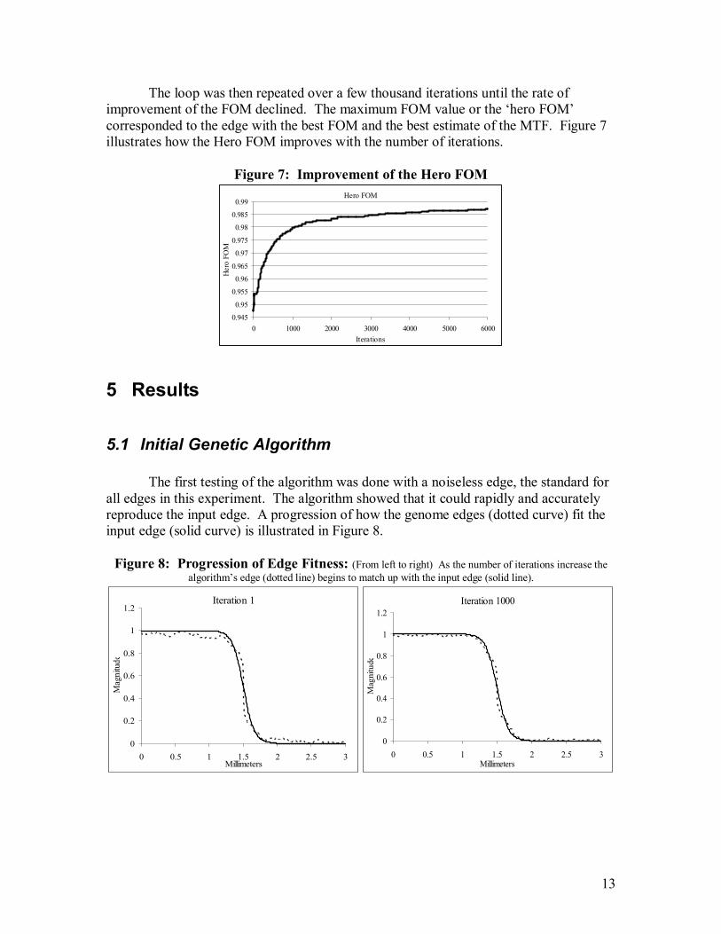
The loop was then repeated over a few thousand iterations until the rate of improvement of the FOM declined. The maximum FOM value or the ‘hero FOM’ corresponded to the edge with the best FOM and the best estimate of the MTF. Figure 7 illustrates how the Hero FOM improves with the number of iterations.
Figure 7: Improvement of the Hero FOM
Hero FOM
0.945
0.95
0.955
0.96
0.965
0.97
0.975
0.98
0.985
0.99
0 1000 2000 3000 4000 5000 6000Iterations
Her
o FO
M
5 Results
5.1 Initial Genetic Algorithm The first testing of the algorithm was done with a noiseless edge, the standard for all edges in this experiment. The algorithm showed that it could rapidly and accurately reproduce the input edge. A progression of how the genome edges (dotted curve) fit the input edge (solid curve) is illustrated in Figure 8.
Figure 8: Progression of Edge Fitness: (From left to right) As the number of iterations increase the
algorithm’s edge (dotted line) begins to match up with the input edge (solid line).
Iteration 1
0
0.2
0.4
0.6
0.8
1
1.2
0 0.5 1 1.5 2 2.5 3Millimeters
Mag
nitu
de
Iteration 1000
0
0.2
0.4
0.6
0.8
1
1.2
0 0.5 1 1.5 2 2.5 3Millimeters
Mag
nitu
de

14
Iteration 4000
0
0.2
0.4
0.6
0.8
1
1.2
0 0.5 1 1.5 2 2.5 3Millimeters
Mag
nitu
deIteration 8000
0
0.2
0.4
0.6
0.8
1
1.2
0 0.5 1 1.5 2 2.5 3Millimeters
Mag
nitu
de
However, the corresponding MTF that the algorithm generated was not an accurate estimate of the real MTF. This result is illustrated in Figure 9B.
Figure 9A: Noiseless Edge and GA Edge
A
-0.15
0.05
0.25
0.45
0.65
0.85
1.05
0 0.5 1 1.5 2 2.5 3Millimeters
Mag
nitu
de
Input Edge
GA Edge
Figure 9B: Real MTF and GA MTF
B
-0.75
-0.25
0.25
0.75
1.25
0 1 2 3 4 5
cy/mm
MTF
GA MTF
Real MTF
The GA MTF in Figure 9B does produce the correct edge when its inverse FFT is calculated within the algorithm. However, compared to the real MTF it is clearly
15
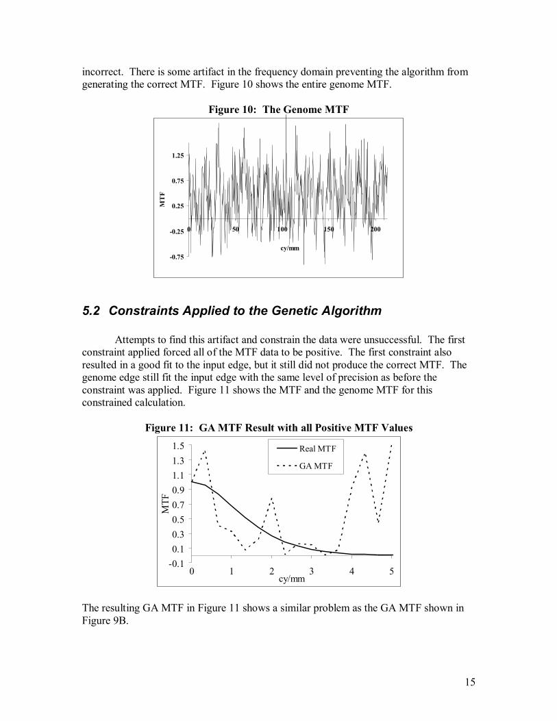
incorrect. There is some artifact in the frequency domain preventing the algorithm from generating the correct MTF. Figure 10 shows the entire genome MTF.
Figure 10: The Genome MTF
-0.75
-0.25
0.25
0.75
1.25
0 50 100 150 200
cy/mm
MT
F
5.2 Constraints Applied to the Genetic Algorithm
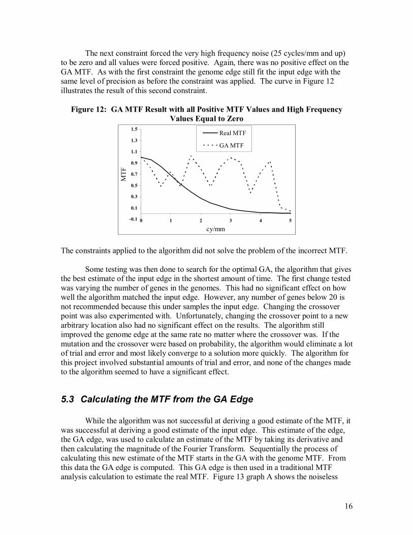
Attempts to find this artifact and constrain the data were unsuccessful. The first constraint applied forced all of the MTF data to be positive. The first constraint also resulted in a good fit to the input edge, but it still did not produce the correct MTF. The genome edge still fit the input edge with the same level of precision as before the constraint was applied. Figure 11 shows the MTF and the genome MTF for this constrained calculation.
Figure 11: GA MTF Result with all Positive MTF Values
-0.10.10.30.50.70.91.11.31.5
0 1 2 3 4 5cy/mm
MTF
Real MTF
GA MTF
The resulting GA MTF in Figure 11 shows a similar problem as the GA MTF shown in Figure 9B.
16
The next constraint forced the very high frequency noise (25 cycles/mm and up) to be zero and all values were forced positive. Again, there was no positive effect on the GA MTF. As with the first constraint the genome edge still fit the input edge with the same level of precision as before the constraint was applied. The curve in Figure 12 illustrates the result of this second constraint.
Figure 12: GA MTF Result with all Positive MTF Values and High Frequency
Values Equal to Zero
-0.1
0.1
0.3
0.5
0.7
0.9
1.1
1.3
1.5
0 1 2 3 4 5
cy/mm
MTF
Real MTF
GA MTF
The constraints applied to the algorithm did not solve the problem of the incorrect MTF. Some testing was then done to search for the optimal GA, the algorithm that gives the best estimate of the input edge in the shortest amount of time. The first change tested was varying the number of genes in the genomes. This had no significant effect on how well the algorithm matched the input edge. However, any number of genes below 20 is not recommended because this under samples the input edge. Changing the crossover point was also experimented with. Unfortunately, changing the crossover point to a new arbitrary location also had no significant effect on the results. The algorithm still improved the genome edge at the same rate no matter where the crossover was. If the mutation and the crossover were based on probability, the algorithm would eliminate a lot of trial and error and most likely converge to a solution more quickly. The algorithm for this project involved substantial amounts of trial and error, and none of the changes made to the algorithm seemed to have a significant effect.
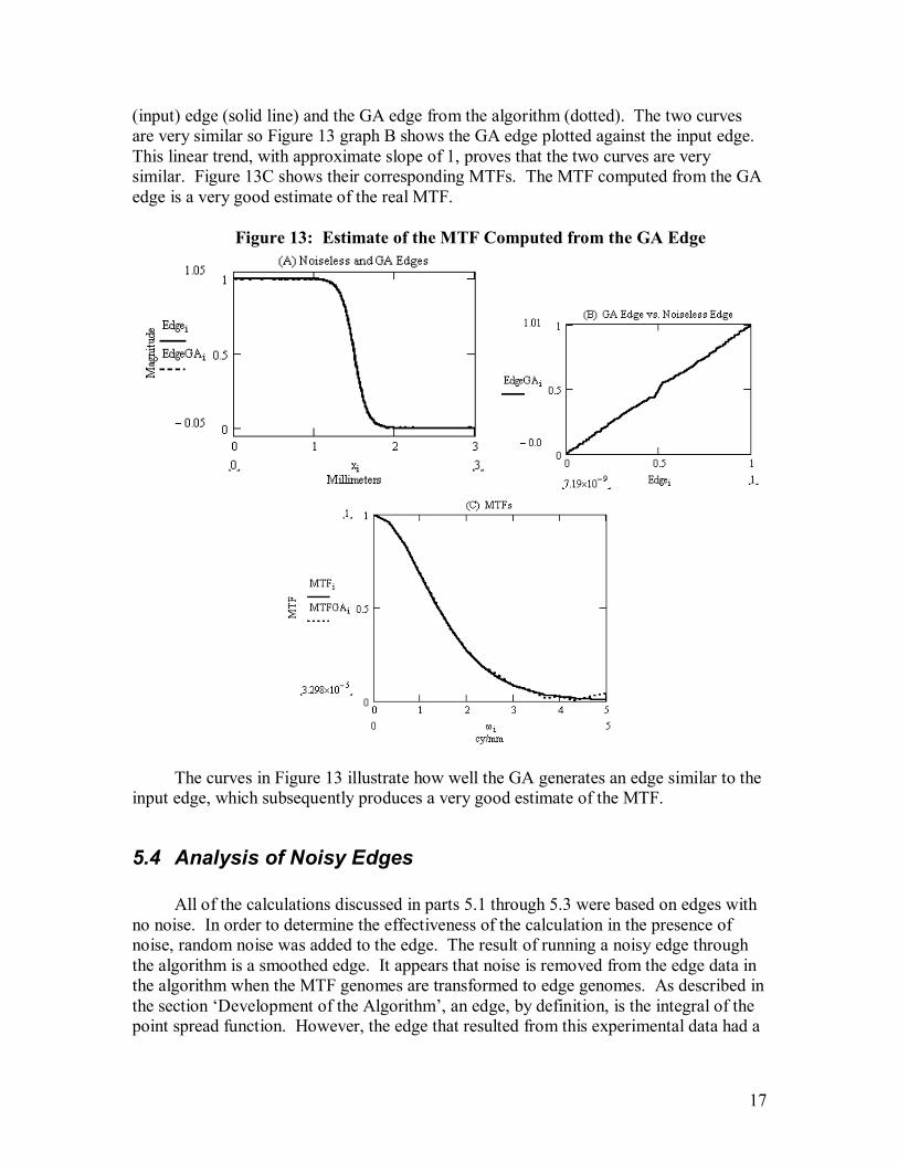
5.3 Calculating the MTF from the GA Edge While the algorithm was not successful at deriving a good estimate of the MTF, it was successful at deriving a good estimate of the input edge. This estimate of the edge, the GA edge, was used to calculate an estimate of the MTF by taking its derivative and then calculating the magnitude of the Fourier Transform. Sequentially the process of calculating this new estimate of the MTF starts in the GA with the genome MTF. From this data the GA edge is computed. This GA edge is then used in a traditional MTF analysis calculation to estimate the real MTF. Figure 13 graph A shows the noiseless
17
(input) edge (solid line) and the GA edge from the algorithm (dotted). The two curves are very similar so Figure 13 graph B shows the GA edge plotted against the input edge. This linear trend, with approximate slope of 1, proves that the two curves are very similar. Figure 13C shows their corresponding MTFs. The MTF computed from the GA edge is a very good estimate of the real MTF.
Figure 13: Estimate of the MTF Computed from the GA Edge
The curves in Figure 13 illustrate how well the GA generates an edge similar to the input edge, which subsequently produces a very good estimate of the MTF.
5.4 Analysis of Noisy Edges
All of the calculations discussed in parts 5.1 through 5.3 were based on edges with no noise. In order to determine the effectiveness of the calculation in the presence of noise, random noise was added to the edge. The result of running a noisy edge through the algorithm is a smoothed edge. It appears that noise is removed from the edge data in the algorithm when the MTF genomes are transformed to edge genomes. As described in the section ‘Development of the Algorithm’, an edge, by definition, is the integral of the point spread function. However, the edge that resulted from this experimental data had a

18
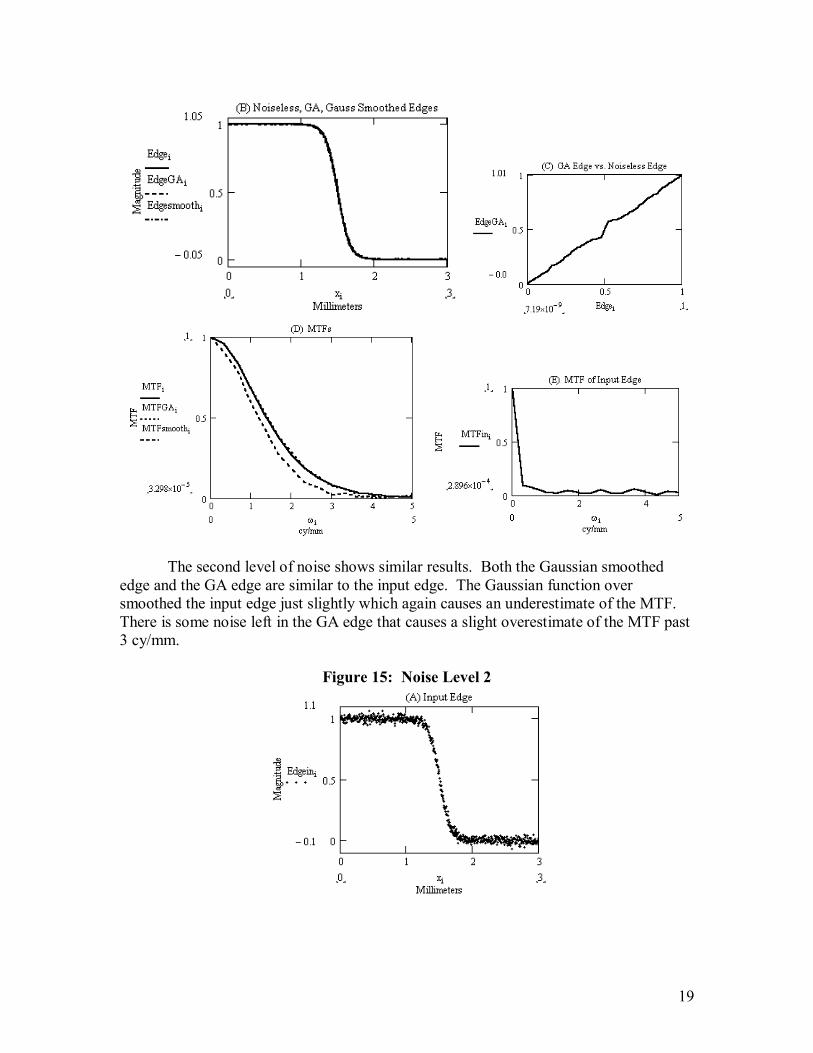
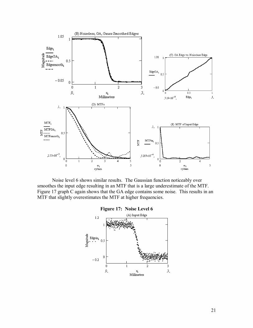
linear trend to it. Subtracting out this linear trend removes the noise. The linear trend changes after each iteration, so it is subtracted out for each generation. The GA edges were used in a traditional calculation to find an estimate of the MTF. This technique gives a very good estimate of the MTF, even when the input is a very noisy edge. The estimate is especially good for MTF values from 1 down to 0.05. Comparing these results to the MTFs calculated from edges smoothed with a Gaussian function shows that this technique gives a much better estimate of the noiseless MTF. Figures 14 through 20 show the results for all 7 noisy edges. The graphs marked (A) show the input noisy edge. The graphs marked (B) show the noiseless edge (solid line), the GA edge (dashed line), and the Gaussian smoothed edge (dashed and dotted line). The graphs marked (C) show the relationship between the GA edge and the noiseless edge. The graphs marked (D) show the real MTF (solid line), the MTF calculated from the GA edge (dotted line), and the MTF calculated from the Gaussian smoothed edge (dashed line). The final graphs marked (E) show the MTF calculated from the noisy input edge For the first level of noise the GA is able to produce an edge that is highly similar to the noiseless edge. The Gaussian smoothed edge is also highly similar to the noiseless edge. These results are reasonable because not much smoothing is done to the input edge in either case. These results are shown in Figure 14 graph B. The MTF calculated from the GA edge is a very good estimate of the MTF. In contrast the MTF calculated from the Gaussian smoothed edge underestimates the MTF, (Figure 14 graph D). Even a very slight change in the edge causes a noticeable change in the MTF. .
Figure 14: Noise Level 1
19
The second level of noise shows similar results. Both the Gaussian smoothed edge and the GA edge are similar to the input edge. The Gaussian function over smoothed the input edge just slightly which again causes an underestimate of the MTF. There is some noise left in the GA edge that causes a slight overestimate of the MTF past 3 cy/mm.
Figure 15: Noise Level 2

20
For the fourth level of noise, the GA edge is not as smooth as would be desirable. Again, this causes the MTF calculated from this edge to be an overestimate of the MTF. Figure 16 graph C also shows that the edge is not completely smooth. The relationship between the GA edge and the noiseless edge is not a simple linear relationship. For this noise level the Gaussian smoothed edge also produces an MTF that underestimates the MTF.
Figure 16: Noise Level 4
21
Noise level 6 shows similar results. The Gaussian function noticeably over smoothes the input edge resulting in an MTF that is a large underestimate of the MTF. Figure 17 graph C again shows that the GA edge contains some noise. This results in an MTF that slightly overestimates the MTF at higher frequencies.
Figure 17: Noise Level 6
22
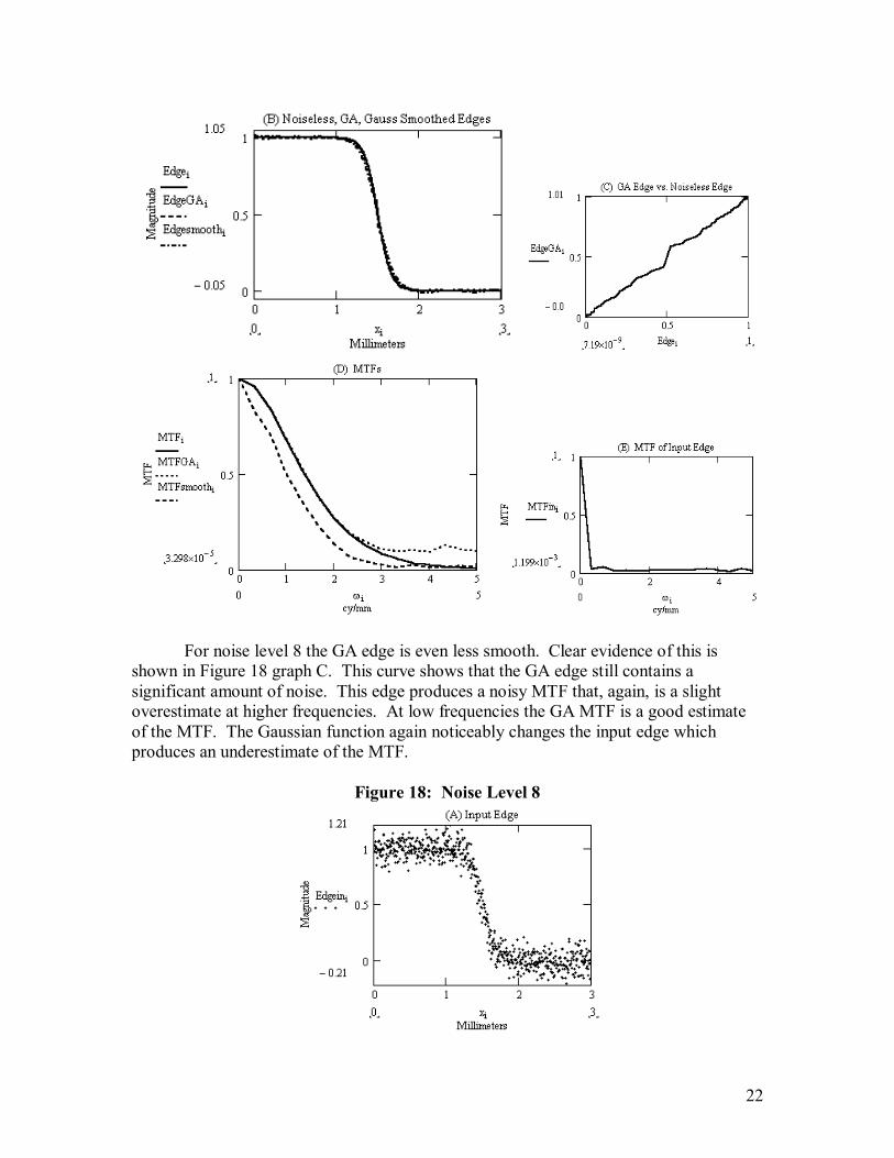
For noise level 8 the GA edge is even less smooth. Clear evidence of this is shown in Figure 18 graph C. This curve shows that the GA edge still contains a significant amount of noise. This edge produces a noisy MTF that, again, is a slight overestimate at higher frequencies. At low frequencies the GA MTF is a good estimate of the MTF. The Gaussian function again noticeably changes the input edge which produces an underestimate of the MTF.
Figure 18: Noise Level 8
23
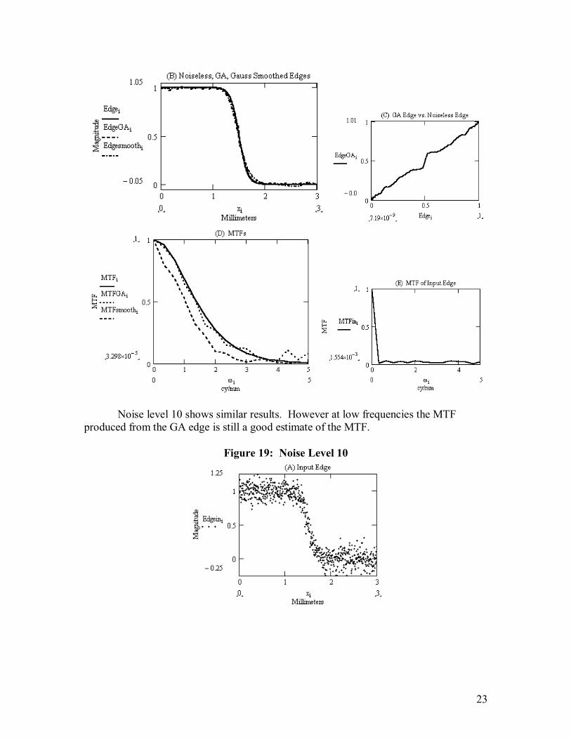
Noise level 10 shows similar results. However at low frequencies the MTF produced from the GA edge is still a good estimate of the MTF.
Figure 19: Noise Level 10

24
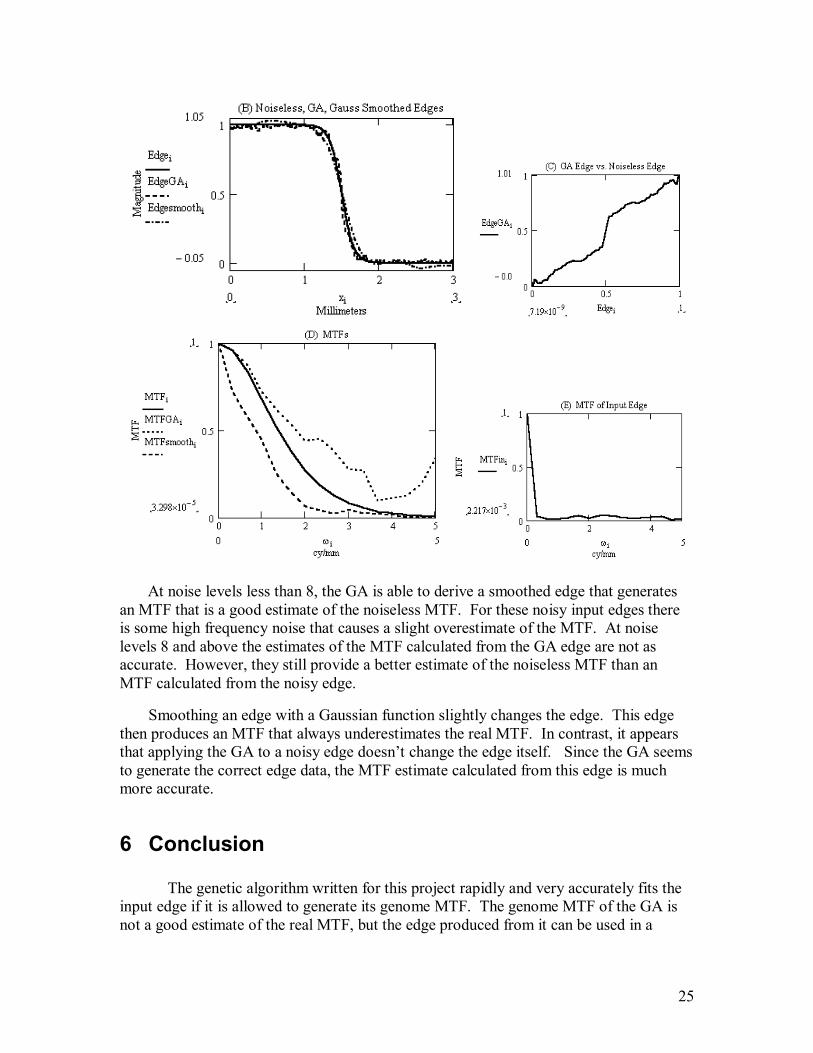
At noise level 20 neither edge produces a very good estimate of the MTF. The GA edge is not smoothed enough causing a gross overestimation of the MTF. The Gaussian smoothed edge is altered too much and therefore produces an underestimate of the MTF.
Figure 20: Noise Level 20
25
At noise levels less than 8, the GA is able to derive a smoothed edge that generates an MTF that is a good estimate of the noiseless MTF. For these noisy input edges there is some high frequency noise that causes a slight overestimate of the MTF. At noise levels 8 and above the estimates of the MTF calculated from the GA edge are not as accurate. However, they still provide a better estimate of the noiseless MTF than an MTF calculated from the noisy edge.
Smoothing an edge with a Gaussian function slightly changes the edge. This edge then produces an MTF that always underestimates the real MTF. In contrast, it appears that applying the GA to a noisy edge doesn’t change the edge itself. Since the GA seems to generate the correct edge data, the MTF estimate calculated from this edge is much more accurate.
6 Conclusion The genetic algorithm written for this project rapidly and very accurately fits the input edge if it is allowed to generate its genome MTF. The genome MTF of the GA is not a good estimate of the real MTF, but the edge produced from it can be used in a

26
traditional MTF analysis. Concerning noisy edges, the GA edge produces a much better estimate of the noiseless MTF than an MTF calculated from a Gaussian smoothed edge. This technique is very useful if the noiseless estimate of the MTF is desired and only a noisy edge is available. There is still much that can be done with this project. It would first be important to determine what causes the incorrect MTF in the algorithm. It is an artifact in the frequency domain that could likely be fixed by padding the vectors with zeroes. If this is corrected then the correct MTF might be found without relying on the traditional MTF analysis. There is also room for improvement in the way the algorithm smoothes the edge because there is still some high frequency noise that remains in the MTF estimate. Finally there are also many more changes that can be made to the algorithm to improve its efficiency. There are different breeding and mutation techniques based on probability that would improve the algorithms performance. This is a promising technique that can certainly be improved in order to expand its applications.

27
7 Appendix
7.1 Computational Details
The data described and explained in the section ‘Results’ was obtained using the Matlab code given in Appendix 7.2.
This code used 50 MTF genomes with 640 genes in each, to match the vector dimension of the synthetic edge data.
The MTF genomes each had their first value equal to 1. The rest of the first 1/4th of
the genes were random numbers between 0 and 1. The next 1/4th of the genes were equal to zero. The next ½ of the genomes were a mirror image of the first ½.
8000 iterations of the loop were used to produce data. The average and hero FOM values were written to file every iteration. The best
MTF and edge genomes were written to file every 10th iteration. The crossover point for breeding was chosen to be the midpoint of the sub-matrix
used for breeding. The first gene value, equal to 1, was not included in the crossover to preserve its value.
The mutation matrix consisted of random numbers with a zero mean and standard
deviation of 0.005. All MTF genome values less than zero were set equal to zero.
7.2 Matlab Source Code %%Create MTF vectors with Random Number Generator%% NumGenes = 640; NumGenomes = 50; %%Create the left half of the MTF matrix%% MTFHalf = [ones(NumGenomes,1) rand(NumGenomes,(NumGenes/4)-1) zeros(NumGenomes,NumGenes/4)]; %%Duplicate the left half to create the right half%% MTF = [MTFHalf fliplr(MTFHalf)]; %%Open Simulated ESF data for comparison%% Data = xlsread('Edge File.xls'); ESF = Data'; subplot(2,2,1); plot(ESF), title('Test Edge Data') %%%%%%%%%%%%%%%%%%%%%%%%%%%%Start Loop%%%%%%%%%%%%%%%%%%%%%%%%%%%%%%%%%% %%Initialize best fitness (Hero) and best Genome (parent)%%
28
HeroFOM = 0.0; BestGenome = []; z = []; fid1 = fopen('MTFData.dat', 'w'); fid2 = fopen('EdgeData.dat', 'w'); fid3 = fopen('FitnessStats.dat', 'w'); NumRuns = 6000; for z = 1:NumRuns %%Take the Inverse Fourier Transform of the MTF vectors%% %%Obtain the magnitude of the transformed data%% for x = 1:NumGenomes Spatial(x,:) = ifft(MTF(x,:)); WorkingPSF(x,:) = abs(Spatial(x,:)); PSF(x,:) = ifftshift(WorkingPSF(x,:)); end subplot(2,2,2); plot(PSF(1,:)), title('Line Spread Function') %%Integrate the PSF to get an Edge%% for x = 1:NumGenomes EdgeData(x,:) = cumsum(PSF(x,:)); end subplot(2,2,3); plot(EdgeData(1,:)), title('Integrated LSF') %%Subtract out Linear Trend%% pt = 32; for x = 1:NumGenomes slope(x) = (EdgeData(x,pt)-EdgeData(x,1))/(pt-1); Y_intercept(x) = -pt*slope(x) + EdgeData(x,pt); end for x = 1:NumGenomes for y = 1:NumGenes NewEdgeData(x,y) = EdgeData(x,y) - (slope(x)*y+Y_intercept(x)); end end %%Take the Magnitude%% for x = 1:NumGenomes for y = 1:NumGenes NEdge(x,y) = abs(NewEdgeData(x,y)); end end %%Normalize the edge data and flip it around%% for x = 1:NumGenomes Flipped(x,:) = fliplr(NEdge(x,:)); Edge(x,:) = Flipped(x,:)/(max(Flipped(x,:))); end subplot(2,2,4); plot(Edge(1,:)), title('Generated Edge Data') %%Compute RMS error between generated edge data and real data%% %%Use 1-RMS error as Figure of Merit and put FOM as first number in MTF vectors%% for x = 1:NumGenomes FOM = 1-(sqrt(sum(((ESF-Edge(x,:)).^2)/NumGenes))); MTF_Rank(x,:) = [FOM MTF(x,:)]; Edge_Rank(x,:) = [FOM Edge(x,:)];
29
end %%Find average FOM%% Average_FOM = mean(MTF_Rank(:,1)); %%Find maximum FOM%% Max_FOM = max(MTF_Rank(:,1)); %%Sort MTF vectors based on FOM (worst is top, best is bottom)%% Sorted_MTF_Matrix = sortrows(MTF_Rank); Sorted_Edge_Matrix = sortrows(Edge_Rank); %%Save the best MTF so far in BestGenome%% if (Max_FOM > HeroFOM) HeroFOM = Max_FOM; BestGenome = Sorted_MTF_Matrix(NumGenomes,2:NumGenes+1); end %%Write the latest information out to file%% Outmatrix = [HeroFOM, Average_FOM]; fprintf(fid3, '%.8g\t\t%.8g\n', Outmatrix); %%Write out every 10th iteration%% %Index(z) = floor(z/100); if (floor(z/100)) ~= (floor((z-1)/100)) fprintf(fid1, '%.8g\n', BestGenome); fprintf(fid2, '%.8g\n', (Sorted_Edge_Matrix(NumGenomes,2:NumGenes+1))); end %%Take FOM values out of MTF vectors%% Parents = Sorted_MTF_Matrix(:,2:NumGenes+1); %%Crossover genes of best 2 data vectors and replace 2 worst vectors%% Children = Parents(:,1:NumGenes/4); CutPoint = 80; start = 2; finish = (NumGenes/4)-1; Children(1,start:CutPoint) = Parents(NumGenomes-1,start:CutPoint); Children(1,CutPoint:finish) = Parents(NumGenomes,CutPoint:finish); Children(2,start:CutPoint) = Parents(NumGenomes,start:CutPoint); Children(2,CutPoint:finish) = Parents(NumGenomes-1,CutPoint:finish); %%Add mutation%% Mutation = [zeros(NumGenomes,1) normrnd(0,.005,NumGenomes,(NumGenes/4)-1)]; Mutated_MTF = Mutation + Children; for x = 1:NumGenomes for y = 1:(NumGenes/4) if Mutated_MTF(x,y) < 0 Mutated_MTF(x,y) = 0; end end end NewChildren = [Mutated_MTF zeros(NumGenomes,NumGenes/2) fliplr(Mutated_MTF)]; MTF = NewChildren; end fclose(fid1); fclose(fid2); fclose(fid3);

30
8 References
1. J.S. Arney, J. Chauvin, J. Nauman, and P.G. Anderson, Kubelka-Munk Theory and the MTF of Paper, J. Imaging Science and Technology. 47, 4 (2003).
2. R. Barakat, Determination of the Optical Transfer Function Directly from the Edge Spread Function, J. Optical Society of America. 55, 10 (1965).
3. D.E. Goldberg, Genetic Algorithms in Search, Optimization & Machine Learning. Addison Wesley Longman Inc. Boston, MA., 1989