a genetic algorithm for the two-dimensional knapsack ... · the 2d knapsack problem is np hard (cf....

Diskussionsbeiträge der Fakultät für Wirtschaftswissenschaft der FernUniversität in Hagen

Herausgegeben von der Dekanin der Fakultät

Alle Rechte liegen bei den Autoren

A Genetic Algorithm for the Two-Dimensional Knapsack Problem

with Rectangular Pieces

Andreas Bortfeldt, Tobias Winter

Diskussionsbeitrag Nr. 425 Mai 2008

2

A Genetic Algorithm for the Two-Dimensional Knapsack Problem with Rectangular Pieces


Abstract:

Given a set of rectangular pieces and a rectangular container, the two-dimensional knapsack problem (2D-KP) consists of orthogonally packing a subset of the pieces within the container such that the sum of the values of the packed pieces is maximized. If the value of a piece is given by its area the objective is to maximize the covered area of the container. A genetic algorithm (GA) is proposed addressing the guillotine case of the 2D-KP as well as the non-guillotine case. Moreover, an orientation constraint may optionally be taken into account and the given piece set may be constrained or unconstrained. The GA is subjected to an extensive test using well-known benchmark instances. In a comparison to recently published methods the GA yields competitive results.

Keywords:

Packing; two-dimensional knapsack problem; rectangular pieces; Single Large Object Placement Problem (SLOPP); Single Knapsack Problem (SKP); genetic algorithm.

Fakultät für Wirtschaftswissenschaft, FernUniversität in Hagen

Profilstr. 8, D-58084 Hagen, BRD

Tel.: 02331/987–4433

Fax: 02331/987–4447

E-Mail: [email protected]

3

A Genetic Algorithm for the Two-Dimensional Knapsack Problem with Rectangular Pieces


1 Introduction

Two-dimensional cutting and packing problems (C&P) are highly relevant in production and logistics. 2D cutting problems are found in customizing material in the glass, steel, wood and paper industries. 2D packing problems result, for example, where goods have to be packed on pallets in horizontal layers. And the space-saving arrangement of adverts on the pages of newspapers, or the effective positioning of components on chips when designing integrated circuits, lead to 2D packing problems.

This paper deals with the two-dimensional knapsack problem (2D-KP) with a set of small rectangular pieces and a larger rectangle, known as a container. The search is for a feasible arrangement of a subset of the pieces in the container that maximizes the total value of the packed pieces. If the value of a piece is given by its area, the aim is to maximize the covered area of the container. An arrangement of pieces, also known as a packing plan, is regarded as feasible if each piece is placed orthogonally (i.e. parallel to the container edges), is completely inside the container and if no two placed pieces overlap. The type of the piece is defined by its two side dimensions and by the value; two copies of a type therefore coincide with regard to the features referred to. The store of pieces is given by a set of piece types, and there are three variants of the 2D-KP in the literature with regard the number of copies per type (cf. Beasley 2004):

(1) Unconstrained knapsack problem (UC) With the unconstrained 2D-KP the number of copies per type is not fixed. A packing plan can therefore have any number of pieces of a type.

(2) Constrained knapsack problem (C) With the constrained 2D-KP an upper limit of copies Pi (Pi > 0) is fixed for at least one piece type i. A packing plan may therefore contain maximal Pi rectangles of type i.

(3) Doubly-constrained knapsack problem (DC) With the doubly-constrained 2D-KP an upper limit of Pi copies is fixed for at least one piece type i and a lower limit Qj is fixed for at least one piece type j (Pi > 0, Qj > 0). A packing plan may therefore have at the most Pi rectangles of type i and at the same time must contain at least Qj rectangles of type j (where applicable, Pi ≤ Qi must apply).

With regard to the stock of small objects, with C&P problems it is usual to differentiate between the variants homogeneous (only one piece type), weakly heterogeneous (few piece types, many copies per type) and strongly heterogeneous (many piece types, a few copies per type). In accordance with these variants differentiated problem types as well are introduced with the new C&P typology from Wäscher et al. (2007). In the given case there is a two-dimensional Single Large Object Placement Problem (SLOPP), with a weakly heterogeneous stock of pieces, and a Single Knapsack Problem (SKP) with an strongly heterogeneous stock of pieces. The following relations appear to apply: with the stock of pieces variants (C) and (DC) there may be both a SLOPP and a SKP, whereas with variant (UC) only a SLOPP should be assumed. In addition, two constraints above all are included in the problem in the literature:

4

(C1) Orientation constraint While turning the pieces by 90° in the container area is generally feasible, the orientation constraint fixes the orientation of all pieces and forbids their rotation.

(C2) Guillotine cutting constraint This constraint demands that all placed pieces are reproducible through a series of guillotine cuts. As is known, a guillotine cut through a rectangle runs from one edge to the opposite edge and parallel to the other two edges of the rectangle.

Both the orientation constraint and the guillotine cutting constraint are found with the customizing of material and are contingent upon, for example, the surface quality of the material (e.g. as a result of rolling) or of the cutting technology used. The orientation constraint is also found with packing problems, for example, the draft layout of pages of newspapers referred to above.

Four subtypes of the 2D knapsack problem can be differentiated for a given variant of the stock of pieces taking account of the constraints (C1) and (C2) (cf. Lodi et al. 1999): - RF: Pieces can be rotated by 90° (R), the guillotine cutting constraint is not required (F); - RG: Pieces can be rotated by 90° (R), the guillotine cutting constraint is required (G); - OF: Orientation of all pieces is fixed (O), the guillotine cutting constraint is not required (F); - OG: Orientation of all pieces is fixed (O), the guillotine cutting constraint is required (G).

Of course, a solution that is feasible with regard to subtype OG is also feasible with regard to the other three subtypes. In the same way, a solution that is feasible with regard to subtype OF or with regard to subtype RG is also feasible with regard to subtype RF.

In this paper, the cases of the (simple) limited and the unlimited stock of pieces are considered. At the same time, both the constraints (C1) and (C2) are to be taken into account where necessary. A genetic algorithm (GA) is suggested that can be applied to all four subtypes defined above of the (simple) constrained or the unconstrained 2D knapsack problem.

The next section provides an overview of the literature on the 2D knapsack problem. Then the genetic algorithm will be described. After this the GA is subjected to a test using known benchmark instances, while at the end the paper is summarized.

2 Previous work

The 2D knapsack problem is NP hard (cf. Beasley 2004). For this reason, together with exact methods in recent years metaheuristic methods have increasingly been suggested to solve it. These include genetic algorithms (GA), Simulated Annealing Algorithms (SAA), Tabu Search Algorithms (TSA) and recently Greedy Randomized Adaptive Search Procedures (GRASP) as well. See Glover and Kochenberger (2003) for an introduction to the fundamental metaheuristic strategies. Exact methods for the 2D-KP are represented mainly by tree search (abbreviated TRS) or Branch and Bound methods (B&B); other exact methods are based on dynamic optimization (DO) or are model based methods. However, the approaches referred to above are also found in heuristics (without an optimality guarantee).

Tables 1a and 1b present a selection of the published solution methods for the 2D-KP with rectangular pieces. Additional papers are considered, for example, in Beasley (2004) (subtypes *F, without guillotine cutting constraint) and in Alvarez-Valdes et al. (2002) (subtypes *G). Together with the source, the treated variant of the 2D-KP (stock of pieces variant and subtype, cf. above), as well as the method type (where applicable with reference to an exact method) are given for each method. For most of the methods the maximal size of calculated problem instances, given by the

5

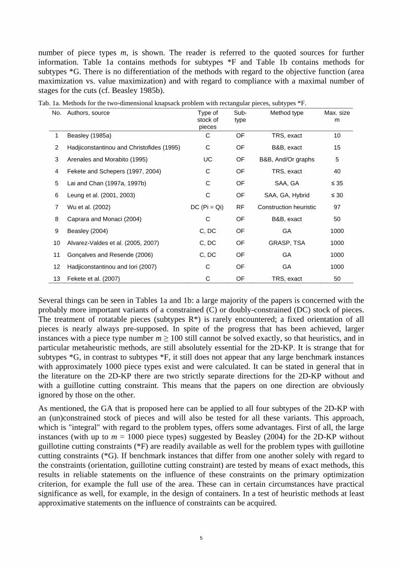
number of piece types m, is shown. The reader is referred to the quoted sources for further information. Table 1a contains methods for subtypes *F and Table 1b contains methods for subtypes *G. There is no differentiation of the methods with regard to the objective function (area maximization vs. value maximization) and with regard to compliance with a maximal number of stages for the cuts (cf. Beasley 1985b). Tab. 1a. Methods for the two-dimensional knapsack problem with rectangular pieces, subtypes *F.

No. Authors, source Type of stock of pieces

Sub-type

Method type Max. size m

1 Beasley (1985a) C OF TRS, exact 10

2 Hadjiconstantinou and Christofides (1995) C OF B&B, exact 15

3 Arenales and Morabito (1995) UC OF B&B, And/Or graphs 5

4 Fekete and Schepers (1997, 2004) C OF TRS, exact 40

5 Lai and Chan (1997a, 1997b) C OF SAA, GA ≤ 35

6 Leung et al. (2001, 2003) C OF SAA, GA, Hybrid ≤ 30

7 Wu et al. (2002) DC (Pi = Qi) RF Construction heuristic 97

8 Caprara and Monaci (2004) C OF B&B, exact 50

9 Beasley (2004) C, DC OF GA 1000

10 Alvarez-Valdes et al. (2005, 2007) C, DC OF GRASP, TSA 1000

11 Gonçalves and Resende (2006) C, DC OF GA 1000

12 Hadjiconstantinou and Iori (2007) C OF GA 1000

13 Fekete et al. (2007) C OF TRS, exact 50

Several things can be seen in Tables 1a and 1b: a large majority of the papers is concerned with the probably more important variants of a constrained (C) or doubly-constrained (DC) stock of pieces. The treatment of rotatable pieces (subtypes R*) is rarely encountered; a fixed orientation of all pieces is nearly always pre-supposed. In spite of the progress that has been achieved, larger instances with a piece type number m ≥ 100 still cannot be solved exactly, so that heuristics, and in particular metaheuristic methods, are still absolutely essential for the 2D-KP. It is strange that for subtypes *G, in contrast to subtypes *F, it still does not appear that any large benchmark instances with approximately 1000 piece types exist and were calculated. It can be stated in general that in the literature on the 2D-KP there are two strictly separate directions for the 2D-KP without and with a guillotine cutting constraint. This means that the papers on one direction are obviously ignored by those on the other.

As mentioned, the GA that is proposed here can be applied to all four subtypes of the 2D-KP with an (un)constrained stock of pieces and will also be tested for all these variants. This approach, which is "integral" with regard to the problem types, offers some advantages. First of all, the large instances (with up to m = 1000 piece types) suggested by Beasley (2004) for the 2D-KP without guillotine cutting constraints (*F) are readily available as well for the problem types with guillotine cutting constraints (*G). If benchmark instances that differ from one another solely with regard to the constraints (orientation, guillotine cutting constraint) are tested by means of exact methods, this results in reliable statements on the influence of these constraints on the primary optimization criterion, for example the full use of the area. These can in certain circumstances have practical significance as well, for example, in the design of containers. In a test of heuristic methods at least approximative statements on the influence of constraints can be acquired.

6

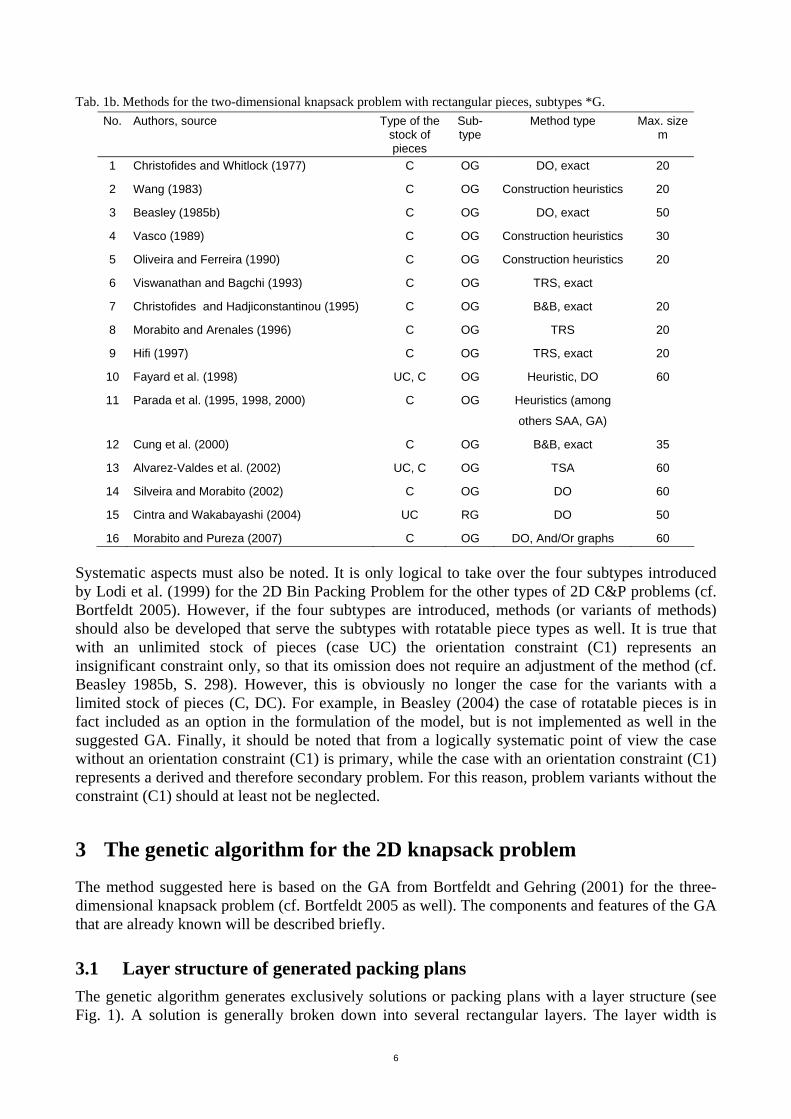
Tab. 1b. Methods for the two-dimensional knapsack problem with rectangular pieces, subtypes *G. No. Authors, source Type of the

stock of pieces

Sub-type

Method type Max. size m

1 Christofides and Whitlock (1977) C OG DO, exact 20

2 Wang (1983) C OG Construction heuristics 20

3 Beasley (1985b) C OG DO, exact 50

4 Vasco (1989) C OG Construction heuristics 30

5 Oliveira and Ferreira (1990) C OG Construction heuristics 20

6 Viswanathan and Bagchi (1993) C OG TRS, exact

7 Christofides and Hadjiconstantinou (1995) C OG B&B, exact 20

8 Morabito and Arenales (1996) C OG TRS 20

9 Hifi (1997) C OG TRS, exact 20

10 Fayard et al. (1998) UC, C OG Heuristic, DO 60

11 Parada et al. (1995, 1998, 2000) C OG Heuristics (among

others SAA, GA)

12 Cung et al. (2000) C OG B&B, exact 35

13 Alvarez-Valdes et al. (2002) UC, C OG TSA 60

14 Silveira and Morabito (2002) C OG DO 60

15 Cintra and Wakabayashi (2004) UC RG DO 50

16 Morabito and Pureza (2007) C OG DO, And/Or graphs 60

Systematic aspects must also be noted. It is only logical to take over the four subtypes introduced by Lodi et al. (1999) for the 2D Bin Packing Problem for the other types of 2D C&P problems (cf. Bortfeldt 2005). However, if the four subtypes are introduced, methods (or variants of methods) should also be developed that serve the subtypes with rotatable piece types as well. It is true that with an unlimited stock of pieces (case UC) the orientation constraint (C1) represents an insignificant constraint only, so that its omission does not require an adjustment of the method (cf. Beasley 1985b, S. 298). However, this is obviously no longer the case for the variants with a limited stock of pieces (C, DC). For example, in Beasley (2004) the case of rotatable pieces is in fact included as an option in the formulation of the model, but is not implemented as well in the suggested GA. Finally, it should be noted that from a logically systematic point of view the case without an orientation constraint (C1) is primary, while the case with an orientation constraint (C1) represents a derived and therefore secondary problem. For this reason, problem variants without the constraint (C1) should at least not be neglected.

3 The genetic algorithm for the 2D knapsack problem

The method suggested here is based on the GA from Bortfeldt and Gehring (2001) for the three-dimensional knapsack problem (cf. Bortfeldt 2005 as well). The components and features of the GA that are already known will be described briefly.

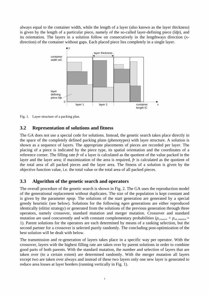
3.1 Layer structure of generated packing plans The genetic algorithm generates exclusively solutions or packing plans with a layer structure (see Fig. 1). A solution is generally broken down into several rectangular layers. The layer width is

7

always equal to the container width, while the length of a layer (also known as the layer thickness) is given by the length of a particular piece, namely of the so-called layer-defining piece (ldp), and its orientation. The layers in a solution follow on consecutively in the lengthways direction (x-direction) of the container without gaps. Each placed piece lies completely in a single layer.

layer 1 layer 2 containerlength lC

x

y

containerwidth wC

layerdefiningpiece ldp

0

layer thickness

Fig. 1. Layer structure of a packing plan.

3.2 Representation of solutions and fitness The GA does not use a special code for solutions. Instead, the genetic search takes place directly in the space of the completely defined packing plans (phenotypes) with layer structure. A solution is shown as a sequence of layers. The appropriate placements of pieces are recorded per layer. The placing of a piece is indicated by the piece type, its spatial orientation and the coordinates of a reference corner. The filling rate fr of a layer is calculated as the quotient of the value packed in the layer and the layer area; if maximization of the area is required, fr is calculated as the quotient of the total area of all packed pieces and the layer area. The fitness of a solution is given by the objective function value, i.e. the total value or the total area of all packed pieces.

3.3 Algorithm of the genetic search and operators The overall procedure of the genetic search is shown in Fig. 2. The GA uses the reproduction model of the generational replacement without duplicates. The size of the population is kept constant and is given by the parameter npop. The solutions of the start generation are generated by a special greedy heuristic (see below). Solutions for the following ngen generations are either reproduced identically (elitist strategy) or generated from the solutions of the previous generation through three operators, namely crossover, standard mutation and merger mutation. Crossover and standard mutation are used concurrently and with constant complementary probabilities (pcrossover + pstd_mutation = 1). Parent solutions for the operators are each determined by means of a ranking selection, but the second partner for a crossover is selected purely randomly. The concluding post-optimization of the best solution will be dealt with below.

The transmission and re-generation of layers takes place in a specific way per operator. With the crossover, layers with the highest filling rate are taken over by parent solutions in order to combine good parts of both parents. With the standard mutation, the number and selection of layers that are taken over (to a certain extent) are determined randomly. With the merger mutation all layers except two are taken over always and instead of these two layers only one new layer is generated to reduce area losses at layer borders (running vertically in Fig. 1).

8

procedure cl_genetic_search(in: problem data, parameters, out: best solution sbest) generate npop solutions for the start generation (with generation counter g = 0); for g := 1 to ngen do reproduce the best nrep solutions of generation g – 1 for generation g; generate npop – nrep solutions for generation g through the operators 'crossover' and 'standard mutation'; carry out nmerge merger mutations and replace in each case the current worst solution ws in

generation g with the mutated solution os, if os is better than ws; endfor;

carry out post-optimization of the previously best solution; end.

Fig. 2. Overall procedure of the genetic search.

3.4 Completing solutions A rump solution created through the transmission of parent layers generally has to be supplemented by several new layers in order to obtain a complete, i.e. no longer extendable, packing plan. The objective of the competent greedy procedure is therefore to supplement a rump solution by several new layers in such a way that the fitness value grows as much as possible.

A single layer is generated in two steps. In step 1 the layer is defined through the selection of a layer-defining piece and its orientation; the layer thickness d is given through the x-dimension of the ldp. A feasible layer definition is found if the ldp is still free (not packed) and if the sum of all layer thicknesses including d does not exceed the container length lC (cf. Fig. 1). In step 2 the defined layer is filled by the ldp and in general further free pieces with a heuristic to be introduced later.

The greedy heuristic for the completion of a rump solution is designed as a tree search with a limited number of successors. First of all, (maximal) n1 first new layers are defined and filled for the incomplete solution sin that is passed on and sin is extended on a trial basis and alternatively by one of these layers. Finally, each of the resulting temporary solutions stmp,1 is supplemented to a complete solution stmp. This is done layer by layer: at maximum n2 new layers are defined and filled for the second, third, etc. new layer; of these, the layer with the maximum filling rate is taken over; the others are "forgotten". Finally, the best obtained complete solution stmp is returned.

The numbers n1 and n2 of successor layers that are taken into account depend on the operator (crossover, mutation variant) that is carried out and result by means of the parameters qldp1 to qldp3 (cf. Bortfeldt 2005). Note that only layers with relatively large layer-defining pieces are included in the competition.

The greedy heuristic is also used to generate the start generation. Here, an empty rump solution sin is assumed and finally the npop best complete solutions stmp are returned.

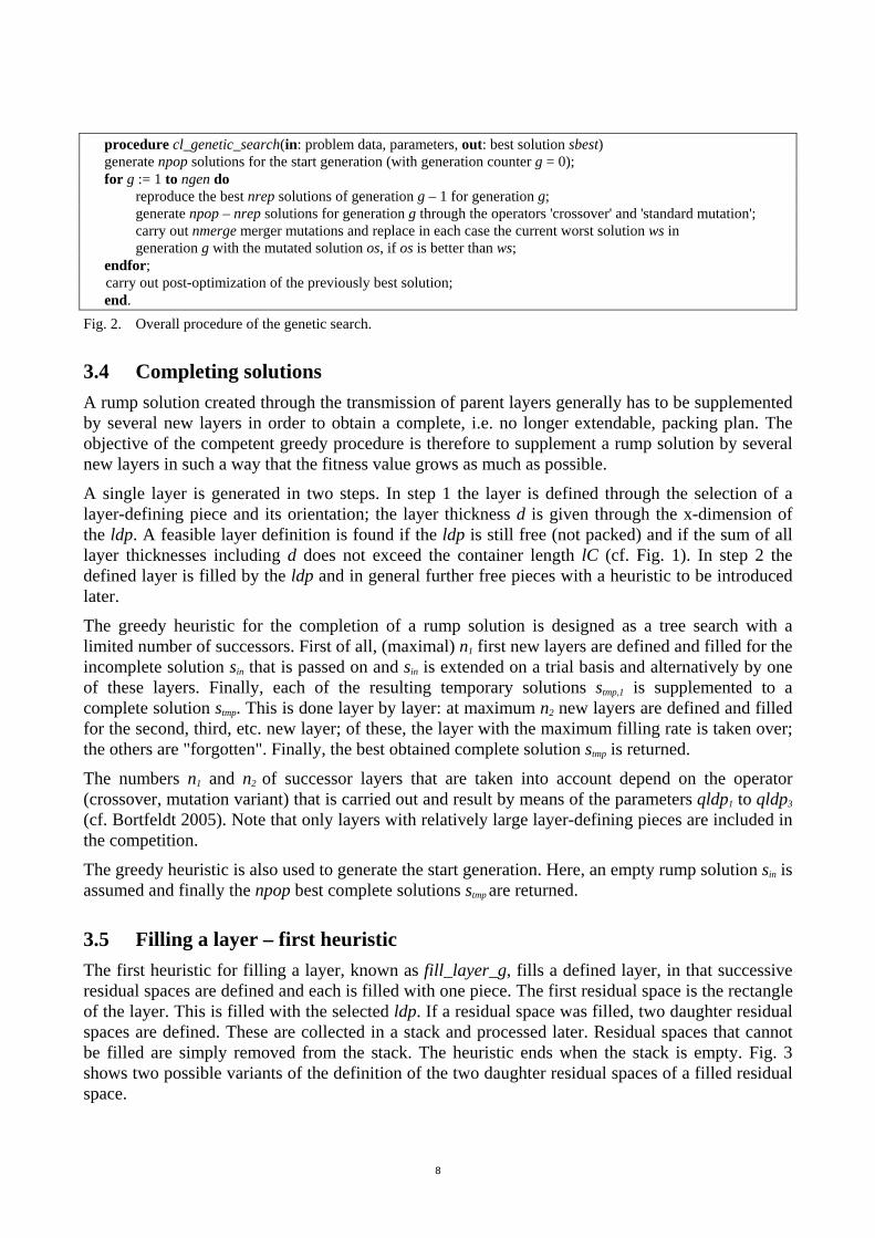
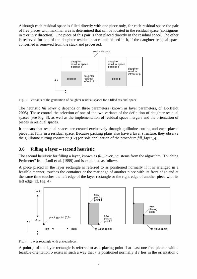
3.5 Filling a layer – first heuristic The first heuristic for filling a layer, known as fill_layer_g, fills a defined layer, in that successive residual spaces are defined and each is filled with one piece. The first residual space is the rectangle of the layer. This is filled with the selected ldp. If a residual space was filled, two daughter residual spaces are defined. These are collected in a stack and processed later. Residual spaces that cannot be filled are simply removed from the stack. The heuristic ends when the stack is empty. Fig. 3 shows two possible variants of the definition of the two daughter residual spaces of a filled residual space.

9

Although each residual space is filled directly with one piece only, for each residual space the pair of free pieces with maximal area is determined that can be located in the residual space (contiguous in x or in y direction). One piece of this pair is then placed directly in the residual space. The other is reserved for one of the daughter residual spaces and placed in it, if the daughter residual space concerned is removed from the stack and processed.

Fig. 3. Variants of the generation of daughter residual spaces for a filled residual space.

The heuristic fill_layer_g depends on three parameters (known as layer parameters, cf. Bortfeldt 2005). These control the selection of one of the two variants of the definition of daughter residual spaces (see Fig. 3), as well as the implementation of residual space mergers and the orientation of pieces in residual spaces.

It appears that residual spaces are created exclusively through guillotine cutting and each placed piece lies fully in a residual space. Because packing plans also have a layer structure, they observe the guillotine cutting constraint (C2) (on sole application of the procedure fill_layer_g).

3.6 Filling a layer – second heuristic The second heuristic for filling a layer, known as fill_layer_ng, stems from the algorithm "Touching Perimeter" from Lodi et al. (1999) and is explained as follows.

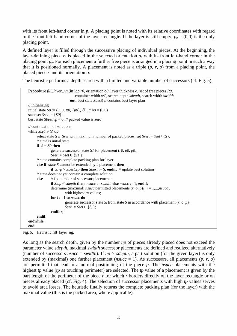
A piece placed in the layer rectangle is referred to as positioned normally if it is arranged in a feasible manner, touches the container or the rear edge of another piece with its front edge and at the same time touches the left edge of the layer rectangle or the right edge of another piece with its left edge (cf. Fig. 4).

Fig. 4. Layer rectangle with placed pieces.

A point p of the layer rectangle is referred to as a placing point if at least one free piece r with a feasible orientation o exists in such a way that r is positioned normally if r lies in the orientation o

10

with its front left-hand corner in p. A placing point is noted with its relative coordinates with regard to the front left-hand corner of the layer rectangle. If the layer is still empty, p0 = (0,0) is the only placing point.

A defined layer is filled through the successive placing of individual pieces. At the beginning, the layer-defining piece r0 is placed in the selected orientation o0 with its front left-hand corner in the placing point p0. For each placement a further free piece is arranged in a placing point in such a way that it is positioned normally. A placement is noted as a triple (p, r, o) from a placing point, the placed piece r and its orientation o.

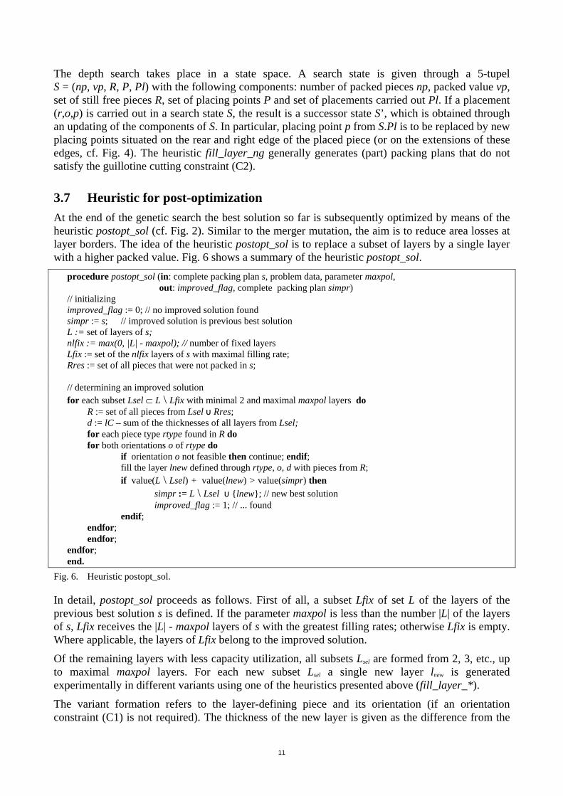
The heuristic performs a depth search with a limited and variable number of successors (cf. Fig. 5).

Procedure fill_layer_ng (in:ldp r0, orientation o0, layer thickness d, set of free pieces R0, container width wC, search depth sdepth, search width swidth, out: best state Sbest) // contains best layer plan

// initializing initial state S0 := (0, 0, R0, {p0}, ∅); // p0 = (0,0) state set Sset := {S0}; best state Sbest.vp = 0; // packed value is zero

// continuation of solutions while Sset ≠ ∅ do select state S ∈ Sset with maximum number of packed pieces, set Sset := Sset \ {S}; // state is initial state

if S = S0 then generate successor state S1 for placement (r0, o0, p0);

Sset := Sset υ {S1 }; // state contains complete packing plan for layer else if state S cannot be extended by a placement then

if S.vp > Sbest.vp then Sbest := S; endif; // update best solution // state does not yet contain a complete solution else // fix number of successor placements

if S.np ≤ sdepth then nsucc := swidth else nsucc := 1; endif; determine (maximal) nsucc permitted placements (r, o, p)i , i = 1,...,nsucc , with highest tp values; for i := 1 to nsucc do generate successor state Si from state S in accordance with placement (r, o, p)i;

Sset := Sset υ {Si }; endfor;

endif; endwhile; end.

Fig. 5. Heuristic fill_layer_ng.

As long as the search depth, given by the number np of pieces already placed does not exceed the parameter value sdepth, maximal swidth successor placements are defined and realized alternatively (number of successors nsucc = swidth). If np > sdepth, a part solution (for the given layer) is only extended by (maximal) one further placement (nsucc = 1). As successors, all placements (p, r, o) are permitted that lead to a normal positioning of the piece p. The nsucc placements with the highest tp value (tp as touching perimeter) are selected. The tp value of a placement is given by the part length of the perimeter of the piece r for which r borders directly on the layer rectangle or on pieces already placed (cf. Fig. 4). The selection of successor placements with high tp values serves to avoid area losses. The heuristic finally returns the complete packing plan (for the layer) with the maximal value (this is the packed area, where applicable).

11

The depth search takes place in a state space. A search state is given through a 5-tupel S = (np, vp, R, P, Pl) with the following components: number of packed pieces np, packed value vp, set of still free pieces R, set of placing points P and set of placements carried out Pl. If a placement (r,o,p) is carried out in a search state S, the result is a successor state S’, which is obtained through an updating of the components of S. In particular, placing point p from S.Pl is to be replaced by new placing points situated on the rear and right edge of the placed piece (or on the extensions of these edges, cf. Fig. 4). The heuristic fill_layer_ng generally generates (part) packing plans that do not satisfy the guillotine cutting constraint (C2).

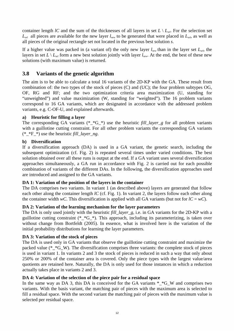
3.7 Heuristic for post-optimization At the end of the genetic search the best solution so far is subsequently optimized by means of the heuristic postopt_sol (cf. Fig. 2). Similar to the merger mutation, the aim is to reduce area losses at layer borders. The idea of the heuristic postopt_sol is to replace a subset of layers by a single layer with a higher packed value. Fig. 6 shows a summary of the heuristic postopt_sol.

procedure postopt_sol (in: complete packing plan s, problem data, parameter maxpol, out: improved_flag, complete packing plan simpr)

// initializing improved_flag := 0; // no improved solution found simpr := s; // improved solution is previous best solution L := set of layers of s; nlfix := max(0, |L| - maxpol); // number of fixed layers Lfix := set of the nlfix layers of s with maximal filling rate; Rres := set of all pieces that were not packed in s; // determining an improved solution for each subset Lsel ⊂ L \ Lfix with minimal 2 and maximal maxpol layers do R := set of all pieces from Lsel υ Rres;

d := lC – sum of the thicknesses of all layers from Lsel; for each piece type rtype found in R do for both orientations o of rtype do if orientation o not feasible then continue; endif;

fill the layer lnew defined through rtype, o, d with pieces from R; if value(L \ Lsel) + value(lnew) > value(simpr) then

simpr := L \ Lsel υ {lnew}; // new best solution improved_flag := 1; // ... found endif;

endfor; endfor; endfor; end.

Fig. 6. Heuristic postopt_sol.

In detail, postopt_sol proceeds as follows. First of all, a subset Lfix of set L of the layers of the previous best solution s is defined. If the parameter maxpol is less than the number |L| of the layers of s, Lfix receives the |L| - maxpol layers of s with the greatest filling rates; otherwise Lfix is empty. Where applicable, the layers of Lfix belong to the improved solution.

Of the remaining layers with less capacity utilization, all subsets Lsel are formed from 2, 3, etc., up to maximal maxpol layers. For each new subset Lsel a single new layer lnew is generated experimentally in different variants using one of the heuristics presented above (fill_layer_*).

The variant formation refers to the layer-defining piece and its orientation (if an orientation constraint (C1) is not required). The thickness of the new layer is given as the difference from the

12

container length lC and the sum of the thicknesses of all layers in set L \ Lsel. For the selection set Lsel all pieces are available for the new layer lnew to be generated that were placed in Lsel, as well as all pieces of the original rectangle set not located in the previous best solution s.

If a higher value was packed in (a variant of) the only new layer lnew than in the layer set Lsel, the layers in set L \ Lsel form a new best solution jointly with layer lnew. At the end, the best of these new solutions (with maximum value) is returned.

3.8 Variants of the genetic algorithm The aim is to be able to calculate a total 16 variants of the 2D-KP with the GA. These result from combination of: the two types of the stock of pieces (C) and (UC); the four problem subtypes OG, OF, RG and RF; and the two optimization criteria area maximization (U, standing for “unweighted”) and value maximization (W, standing for “weighted”). The 16 problem variants correspond to 16 GA variants, which are designated in accordance with the addressed problem variants, e.g. C-OF-U, and explained afterwards.

a) Heuristic for filling a layer The corresponding GA variants (*_*G_*) use the heuristic fill_layer_g for all problem variants with a guillotine cutting constraint. For all other problem variants the corresponding GA variants (*_*F_*) use the heuristic fill_layer_ng.

b) Diversification If a diversification approach (DA) is used in a GA variant, the genetic search, including the subsequent optimization (cf. Fig. 2) is repeated several times under varied conditions. The best solution obtained over all these runs is output at the end. If a GA variant uses several diversification approaches simultaneously, a GA run in accordance with Fig. 2 is carried out for each possible combination of variants of the different DAs. In the following, the diversification approaches used are introduced and assigned to the GA variants.

DA 1: Variation of the position of the layers in the container The DA comprises two variants. In variant 1 (as described above) layers are generated that follow each other along the container length lC (cf. Fig. 1). In variant 2, the layers follow each other along the container width wC. This diversification is applied with all GA variants (but not for lC = wC).

DA 2: Variation of the learning mechanism for the layer parameters The DA is only used jointly with the heuristic fill_layer_g, i.e. in GA variants for the 2D-KP with a guillotine cutting constraint (*_*G_*). This approach, including its parameterizing, is taken over without change from Bortfeldt (2005). In essence, what is involved here is the variation of the initial probability distributions for learning the layer parameters.

DA 3: Variation of the stock of pieces The DA is used only in GA variants that observe the guillotine cutting constraint and maximize the packed value (*_*G_W). The diversification comprises three variants: the complete stock of pieces is used in variant 1. In variants 2 and 3 the stock of pieces is reduced in such a way that only about 250% or 200% of the container area is covered. Only the piece types with the largest value/area quotients are retained here. Naturally, the DA is only used for those instances in which a reduction actually takes place in variants 2 and 3.

DA 4: Variation of the selection of the piece pair for a residual space In the same way as DA 3, this DA is conceived for the GA variants *_*G_W and comprises two variants. With the basis variant, the matching pair of pieces with the maximum area is selected to fill a residual space. With the second variant the matching pair of pieces with the maximum value is selected per residual space.

13

c) Parameterizing The parameterizing of the GA variants can be summarized as follows: - The parameters of the genetic search, namely npop, pcrossover, pstd_mutation, nrep, nmerge, and the

parameters qldpi (i = 1,2,3) for completing solutions, are chosen as in Bortfeldt (2005). - The parameterizing of diversification approaches has already been dealt with. - For the GA variants *_*G_U (for the guillotine cutting constraint, area maximizing) ngen = 1000

generations are generated per GA run. To limit the search effort and, e.g., because of the large-scale diversification ngen = 20 is chosen for all other GA variants.

- For the heuristic fill_layer_ng the parameter values sdepth = 5 and swidth = 5 are stipulated. For the post-optimization the parameter maxpol is set to 5.

- A time limit per GA run is set as follows: maxtime = 600 seconds (on a 3 GHz PC, see below) for the GA variants *_*G_* (for the guillotine cutting constraint), maxtime = 3600 seconds otherwise.

Altogether there is a standard parameter set available for each GA variant, and the parameter sets of the GA variants largely coincide. d) Orientation constraint If an orientation constraint (C1) is required non-permitted orientations are excluded from the start for layer-defining pieces and for other pieces placed in a layer. Each GA variant "without orientation constraint“ (*_R*_*) coincides with the corresponding GA variant "with orientation constraint“ (*_O*_*), but both possible orientations are permitted per piece type.

e) Unlimited stock of pieces Each GA variant for an unlimited stock of pieces (UC_*_*) coincides with the corresponding GA variant for a limited stock of pieces (C_*_*). With one GA variant of the first group, it is only ensured that the copies per piece type cover the container area to at least 100%.

A single GA run (cf. b) Diversification) ends after all ngen generations (after the start generation) are generated or the time limit maxtime was exceeded. A GA run and the complete procedure break off prematurely after an optimal solution is identified. An optimal solution is recognized by all pieces being packed or the packed value (or the packed area) reaching the upper bound Ub used here. For a detailed definition of Ub see, for example, Gonçalves and Resende (2006). In brief, the upper bound Ub is acquired through a relaxation of the 2D-KP to a constrained 1D knapsack problem. For a concrete 2D-KP instance the value Ub results as an objective function value of the appropriate relaxed 1D-KP instance.

4 Testing the method

The genetic algorithm, referred to below as CLGAL (CL stands for "container loading", L for "layer"), was implemented in C by means of the .NET 2003 environment and tested with an Intel PC (3GHz, Dual Core, 2GB RAM). If the type of the stock of pieces and the target criterion are ascertained, the appropriate GA variants are designated below with the problem subtype, for example CLGAL-OG.

4.1 Problem instances and comparison methods for the test Five sets of benchmark instances for the constrained (C) 2D-KP from the literature were included for the test. The instances of the first four sets were used up to now only as instances of the subtype

14

OF and the instances of the fifth set only considered as instances of the subtype OG. A sixth set of instances is used for testing the GA for the unconstrained (UC) 2D-KP.

a) Set1 Set1 consists of 21 smaller instances. In each case, the packed value (in contrast to the area) is to be maximized and an optimal solution is known for each instance (cf. Beasley 2004). The 21 instances include: 12 from Beasley (1985a), 2 from Hadjiconstantinou and Christofides (1995), 1 from Wang (1983), 1 from Christofides and Whitlock (1977) and 5 from Fekete and Schepers (1997). Where applicable, the designations of instances are taken from the literature (cf. Annex, Table 4).

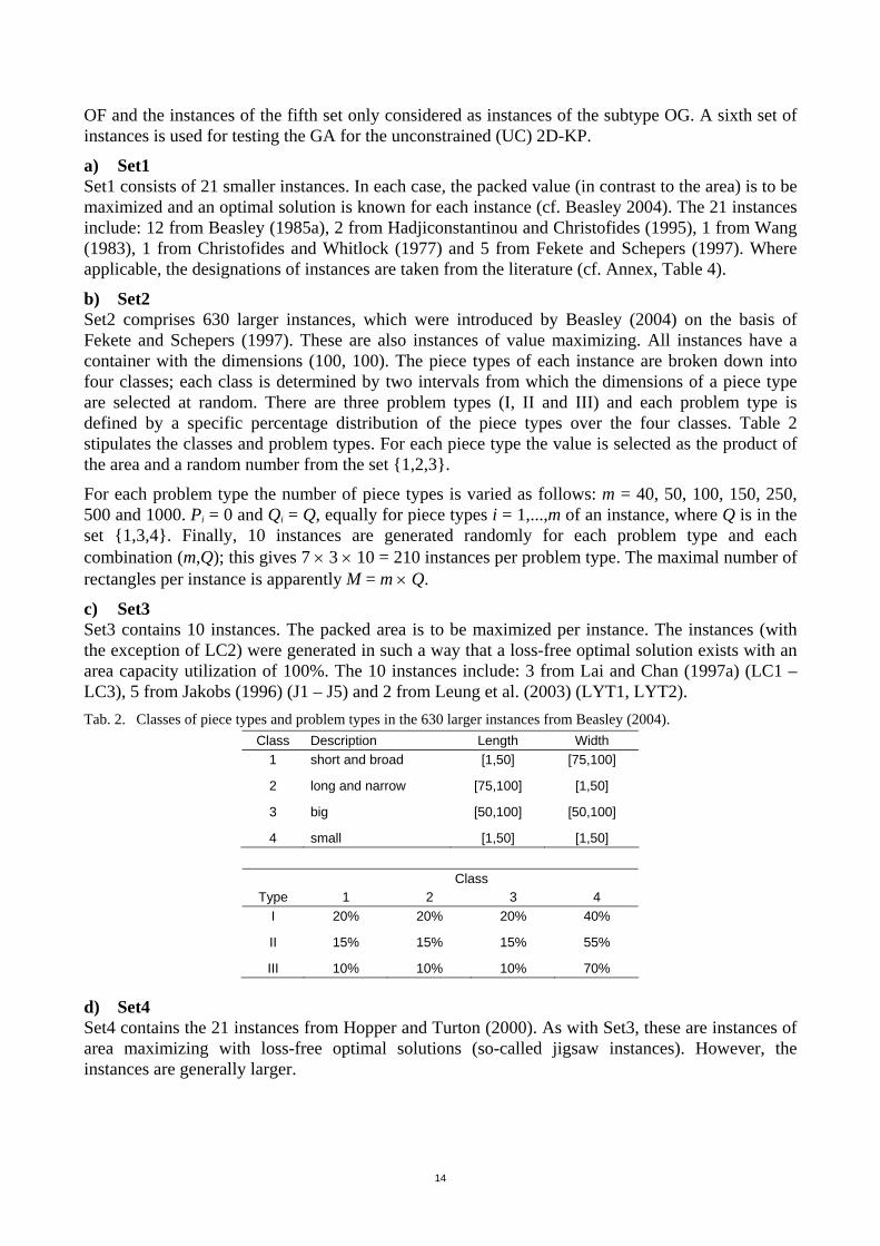
b) Set2 Set2 comprises 630 larger instances, which were introduced by Beasley (2004) on the basis of Fekete and Schepers (1997). These are also instances of value maximizing. All instances have a container with the dimensions (100, 100). The piece types of each instance are broken down into four classes; each class is determined by two intervals from which the dimensions of a piece type are selected at random. There are three problem types (I, II and III) and each problem type is defined by a specific percentage distribution of the piece types over the four classes. Table 2 stipulates the classes and problem types. For each piece type the value is selected as the product of the area and a random number from the set {1,2,3}.

For each problem type the number of piece types is varied as follows: m = 40, 50, 100, 150, 250, 500 and 1000. Pi = 0 and Qi = Q, equally for piece types i = 1,...,m of an instance, where Q is in the set {1,3,4}. Finally, 10 instances are generated randomly for each problem type and each combination (m,Q); this gives 7 × 3 × 10 = 210 instances per problem type. The maximal number of rectangles per instance is apparently M = m × Q.

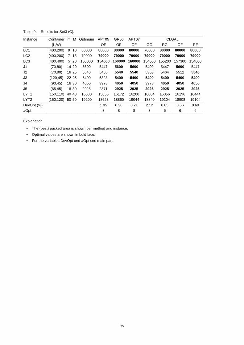
c) Set3 Set3 contains 10 instances. The packed area is to be maximized per instance. The instances (with the exception of LC2) were generated in such a way that a loss-free optimal solution exists with an area capacity utilization of 100%. The 10 instances include: 3 from Lai and Chan (1997a) (LC1 – LC3), 5 from Jakobs (1996) (J1 – J5) and 2 from Leung et al. (2003) (LYT1, LYT2). Tab. 2. Classes of piece types and problem types in the 630 larger instances from Beasley (2004).

Class Description Length Width 1 short and broad [1,50] [75,100]

2 long and narrow [75,100] [1,50]

3 big [50,100] [50,100]

4 small [1,50] [1,50]

Class Type 1 2 3 4

I 20% 20% 20% 40%

II 15% 15% 15% 55%

III 10% 10% 10% 70%

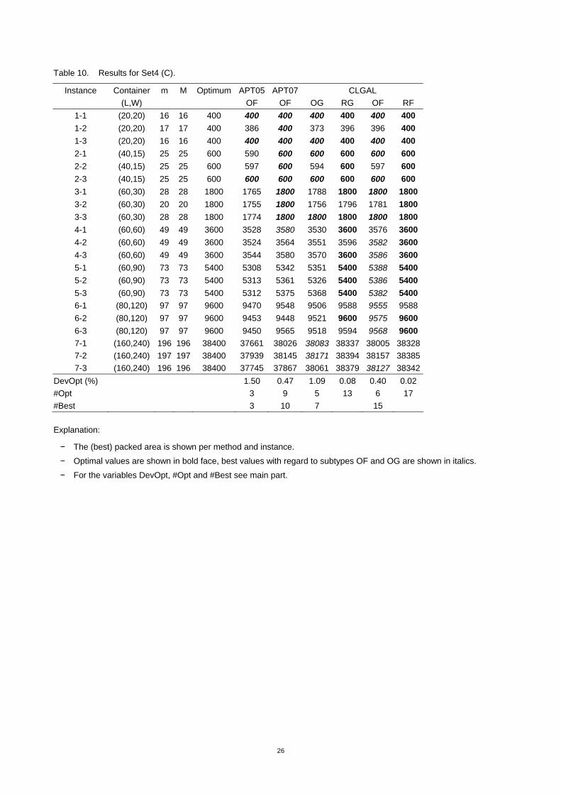
d) Set4 Set4 contains the 21 instances from Hopper and Turton (2000). As with Set3, these are instances of area maximizing with loss-free optimal solutions (so-called jigsaw instances). However, the instances are generally larger.

15

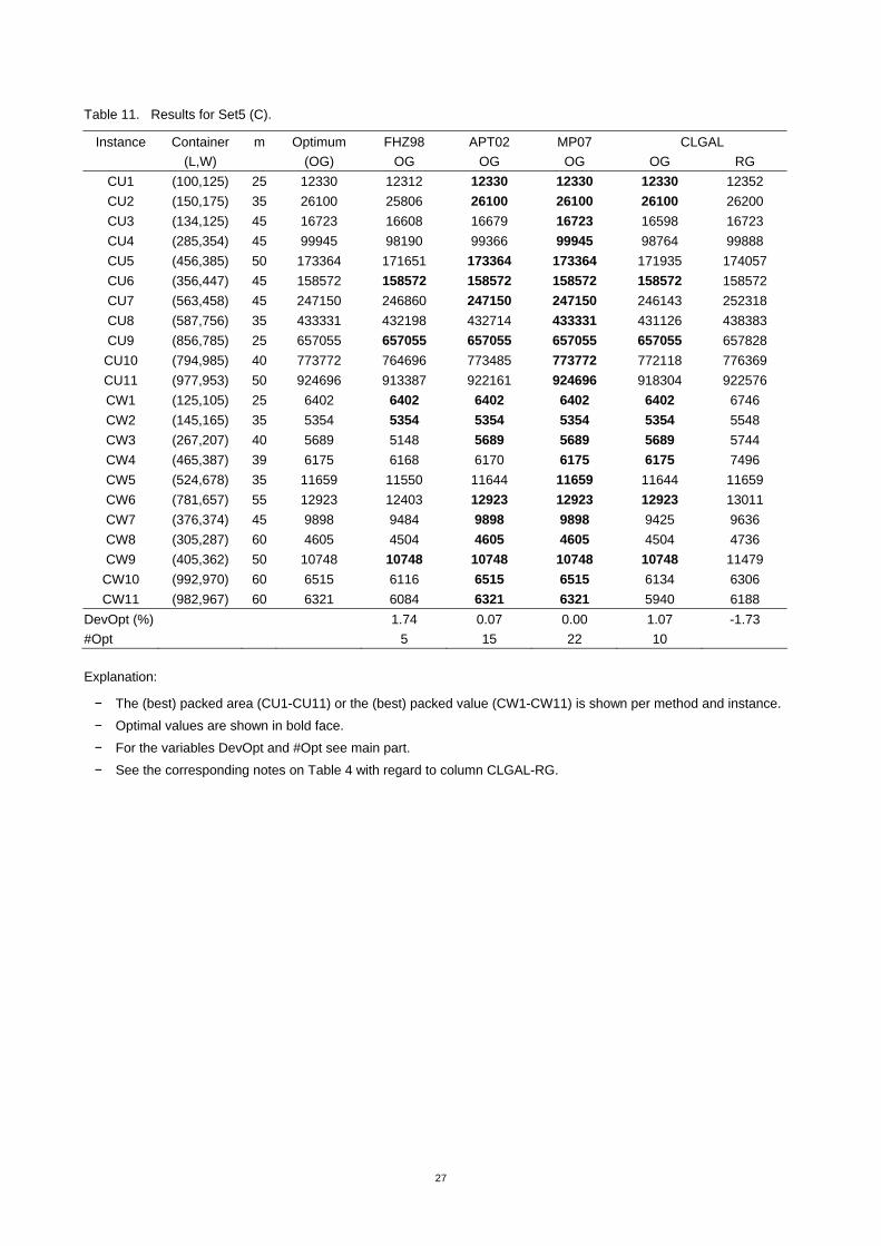
e) Set5 Set5 includes 22 instances from Fayard et al. (1998). In instances CU1 to CU11 the packed area is to be maximized, in instances CW1 to CW11 the packed value. An optimal solution is known for all instances. The numbers of the piece types vary between m = 25 and m = 60; some of the instances belong to the previously largest calculated instances of problem variant OG.

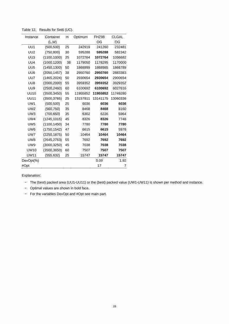
f) Set6 Set6 also includes 22 instances from Fayard et al. (1998) for the unconstrained (UC) 2D-KP. With instances UU1 to UU11 the packed area is to be maximized, in instances UW1 to UW11 the packed value. An optimal solution is known for all instances. The numbers of the piece types vary again between m = 25 and m = 60.

The following comparison methods were included altogether for the first four instances sets: Beasley (2004) (in brief: B04), Alvarez-Valdes et al. (2005) (APT05), Gonçalves and Resende (2006) (GR06), Hadjiconstantinou and Iori (2007) (HI07), and Alvarez-Valdes et al. (2007) (APT07). For the fifth instances set the following methods are used for a comparison: Fayard et al. (1998) (FHZ98), Alvarez-Valdes et al. (2002) (APT02) and Morabito and Pureza (2007) (MP07). For instances set Set6 the GA is only compared to the method from Fayard et al. (1998) (FHZ98).

It is evident that the binding of sets 1 to 4 to the subtype OF or of set 5 to the subtype OG that was referred to earlier is not compulsory. Consequently, to test the GA the instance groups Set1, Set2, Set3 and Set4 were used for all four subtypes and Set5 for the subtypes OG and RG. Set6 is only used for the subtype OG.

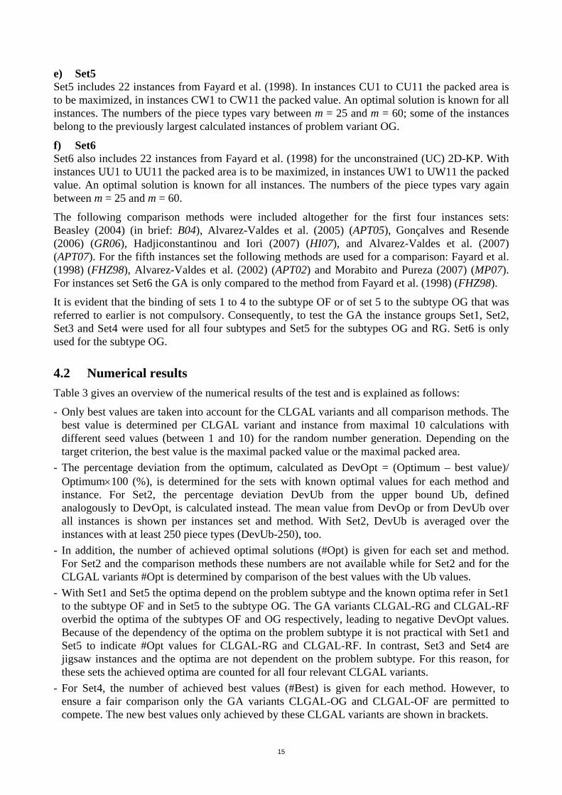
4.2 Numerical results Table 3 gives an overview of the numerical results of the test and is explained as follows:

- Only best values are taken into account for the CLGAL variants and all comparison methods. The best value is determined per CLGAL variant and instance from maximal 10 calculations with different seed values (between 1 and 10) for the random number generation. Depending on the target criterion, the best value is the maximal packed value or the maximal packed area.

- The percentage deviation from the optimum, calculated as DevOpt = (Optimum – best value)/ Optimum×100 (%), is determined for the sets with known optimal values for each method and instance. For Set2, the percentage deviation DevUb from the upper bound Ub, defined analogously to DevOpt, is calculated instead. The mean value from DevOp or from DevUb over all instances is shown per instances set and method. With Set2, DevUb is averaged over the instances with at least 250 piece types (DevUb-250), too.

- In addition, the number of achieved optimal solutions (#Opt) is given for each set and method. For Set2 and the comparison methods these numbers are not available while for Set2 and for the CLGAL variants #Opt is determined by comparison of the best values with the Ub values.

- With Set1 and Set5 the optima depend on the problem subtype and the known optima refer in Set1 to the subtype OF and in Set5 to the subtype OG. The GA variants CLGAL-RG and CLGAL-RF overbid the optima of the subtypes OF and OG respectively, leading to negative DevOpt values. Because of the dependency of the optima on the problem subtype it is not practical with Set1 and Set5 to indicate #Opt values for CLGAL-RG and CLGAL-RF. In contrast, Set3 and Set4 are jigsaw instances and the optima are not dependent on the problem subtype. For this reason, for these sets the achieved optima are counted for all four relevant CLGAL variants.

- For Set4, the number of achieved best values (#Best) is given for each method. However, to ensure a fair comparison only the GA variants CLGAL-OG and CLGAL-OF are permitted to compete. The new best values only achieved by these CLGAL variants are shown in brackets.

16

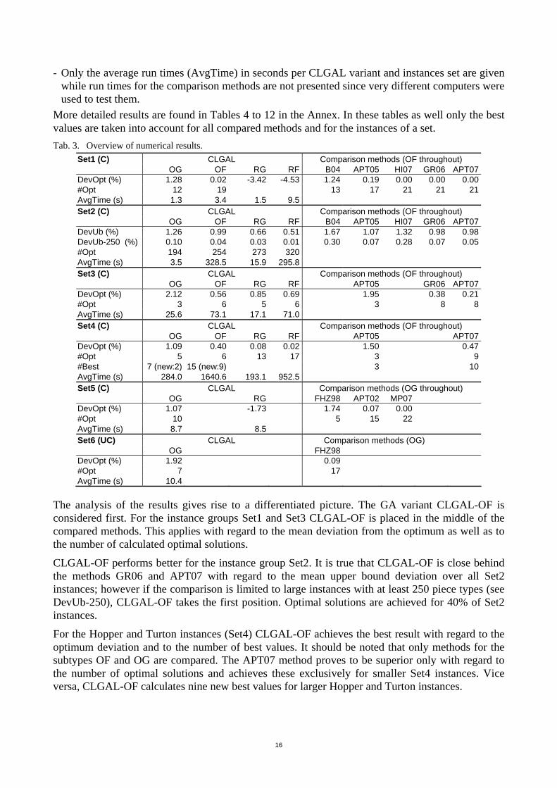
- Only the average run times (AvgTime) in seconds per CLGAL variant and instances set are given while run times for the comparison methods are not presented since very different computers were used to test them.

More detailed results are found in Tables 4 to 12 in the Annex. In these tables as well only the best values are taken into account for all compared methods and for the instances of a set. Tab. 3. Overview of numerical results.

Set1 (C) CLGAL Comparison methods (OF throughout) OG OF RG RF B04 APT05 HI07 GR06 APT07DevOpt (%) 1.28 0.02 -3.42 -4.53 1.24 0.19 0.00 0.00 0.00#Opt 12 19 13 17 21 21 21AvgTime (s) 1.3 3.4 1.5 9.5 Set2 (C) CLGAL Comparison methods (OF throughout) OG OF RG RF B04 APT05 HI07 GR06 APT07DevUb (%) 1.26 0.99 0.66 0.51 1.67 1.07 1.32 0.98 0.98DevUb-250 (%) 0.10 0.04 0.03 0.01 0.30 0.07 0.28 0.07 0.05#Opt 194 254 273 320 AvgTime (s) 3.5 328.5 15.9 295.8 Set3 (C) CLGAL Comparison methods (OF throughout) OG OF RG RF APT05 GR06 APT07DevOpt (%) 2.12 0.56 0.85 0.69 1.95 0.38 0.21#Opt 3 6 5 6 3 8 8AvgTime (s) 25.6 73.1 17.1 71.0 Set4 (C) CLGAL Comparison methods (OF throughout) OG OF RG RF APT05 APT07DevOpt (%) 1.09 0.40 0.08 0.02 1.50 0.47#Opt 5 6 13 17 3 9#Best 7 (new:2) 15 (new:9) 3 10AvgTime (s) 284.0 1640.6 193.1 952.5 Set5 (C) CLGAL Comparison methods (OG throughout) OG RG FHZ98 APT02 MP07 DevOpt (%) 1.07 -1.73 1.74 0.07 0.00 #Opt 10 5 15 22 AvgTime (s) 8.7 8.5 Set6 (UC) CLGAL Comparison methods (OG) OG FHZ98 DevOpt (%) 1.92 0.09 #Opt 7 17 AvgTime (s) 10.4

The analysis of the results gives rise to a differentiated picture. The GA variant CLGAL-OF is considered first. For the instance groups Set1 and Set3 CLGAL-OF is placed in the middle of the compared methods. This applies with regard to the mean deviation from the optimum as well as to the number of calculated optimal solutions.

CLGAL-OF performs better for the instance group Set2. It is true that CLGAL-OF is close behind the methods GR06 and APT07 with regard to the mean upper bound deviation over all Set2 instances; however if the comparison is limited to large instances with at least 250 piece types (see DevUb-250), CLGAL-OF takes the first position. Optimal solutions are achieved for 40% of Set2 instances.

For the Hopper and Turton instances (Set4) CLGAL-OF achieves the best result with regard to the optimum deviation and to the number of best values. It should be noted that only methods for the subtypes OF and OG are compared. The APT07 method proves to be superior only with regard to the number of optimal solutions and achieves these exclusively for smaller Set4 instances. Vice versa, CLGAL-OF calculates nine new best values for larger Hopper and Turton instances.

17

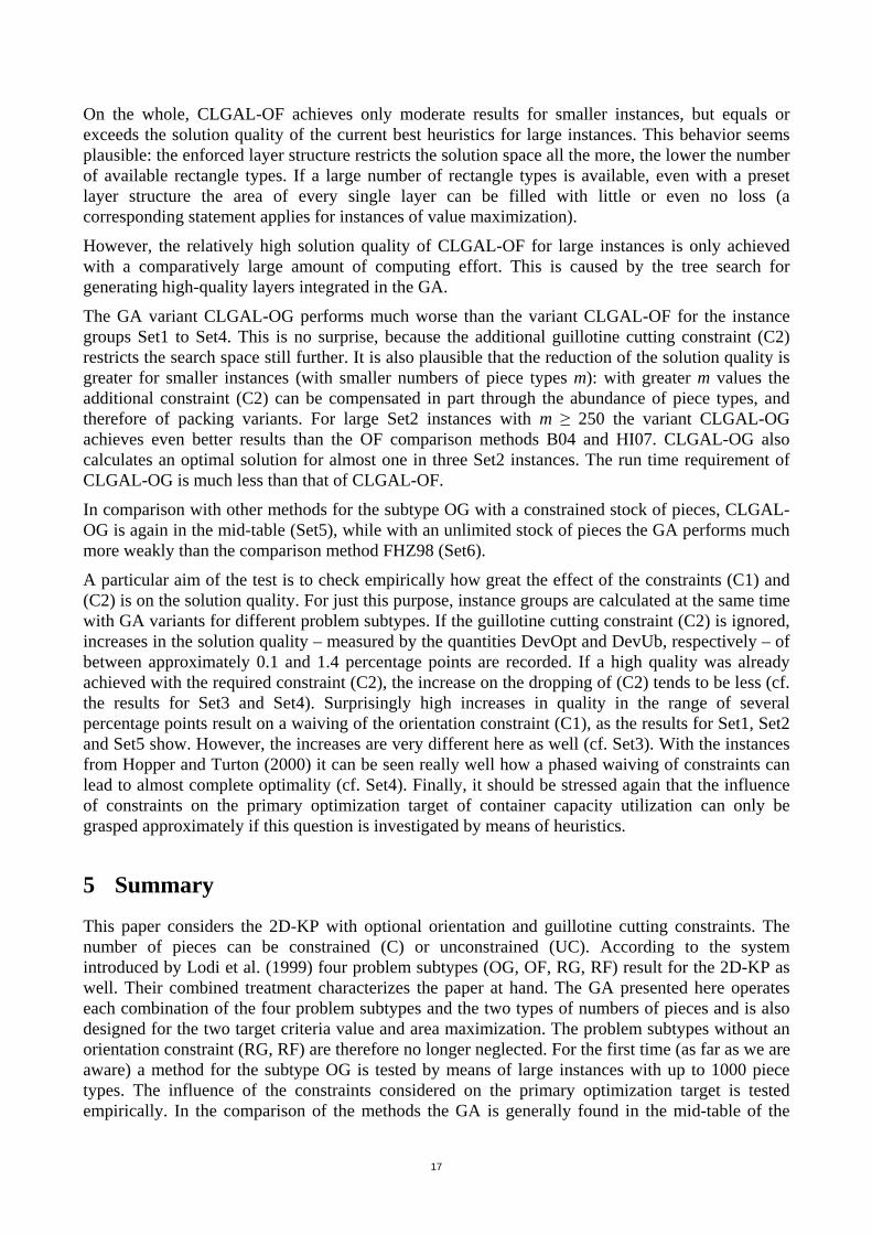
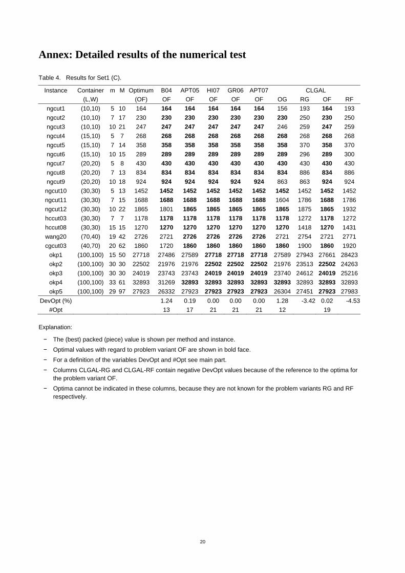
On the whole, CLGAL-OF achieves only moderate results for smaller instances, but equals or exceeds the solution quality of the current best heuristics for large instances. This behavior seems plausible: the enforced layer structure restricts the solution space all the more, the lower the number of available rectangle types. If a large number of rectangle types is available, even with a preset layer structure the area of every single layer can be filled with little or even no loss (a corresponding statement applies for instances of value maximization).

However, the relatively high solution quality of CLGAL-OF for large instances is only achieved with a comparatively large amount of computing effort. This is caused by the tree search for generating high-quality layers integrated in the GA.

The GA variant CLGAL-OG performs much worse than the variant CLGAL-OF for the instance groups Set1 to Set4. This is no surprise, because the additional guillotine cutting constraint (C2) restricts the search space still further. It is also plausible that the reduction of the solution quality is greater for smaller instances (with smaller numbers of piece types m): with greater m values the additional constraint (C2) can be compensated in part through the abundance of piece types, and therefore of packing variants. For large Set2 instances with m ≥ 250 the variant CLGAL-OG achieves even better results than the OF comparison methods B04 and HI07. CLGAL-OG also calculates an optimal solution for almost one in three Set2 instances. The run time requirement of CLGAL-OG is much less than that of CLGAL-OF.

In comparison with other methods for the subtype OG with a constrained stock of pieces, CLGAL-OG is again in the mid-table (Set5), while with an unlimited stock of pieces the GA performs much more weakly than the comparison method FHZ98 (Set6).

A particular aim of the test is to check empirically how great the effect of the constraints (C1) and (C2) is on the solution quality. For just this purpose, instance groups are calculated at the same time with GA variants for different problem subtypes. If the guillotine cutting constraint (C2) is ignored, increases in the solution quality – measured by the quantities DevOpt and DevUb, respectively – of between approximately 0.1 and 1.4 percentage points are recorded. If a high quality was already achieved with the required constraint (C2), the increase on the dropping of (C2) tends to be less (cf. the results for Set3 and Set4). Surprisingly high increases in quality in the range of several percentage points result on a waiving of the orientation constraint (C1), as the results for Set1, Set2 and Set5 show. However, the increases are very different here as well (cf. Set3). With the instances from Hopper and Turton (2000) it can be seen really well how a phased waiving of constraints can lead to almost complete optimality (cf. Set4). Finally, it should be stressed again that the influence of constraints on the primary optimization target of container capacity utilization can only be grasped approximately if this question is investigated by means of heuristics.

5 Summary

This paper considers the 2D-KP with optional orientation and guillotine cutting constraints. The number of pieces can be constrained (C) or unconstrained (UC). According to the system introduced by Lodi et al. (1999) four problem subtypes (OG, OF, RG, RF) result for the 2D-KP as well. Their combined treatment characterizes the paper at hand. The GA presented here operates each combination of the four problem subtypes and the two types of numbers of pieces and is also designed for the two target criteria value and area maximization. The problem subtypes without an orientation constraint (RG, RF) are therefore no longer neglected. For the first time (as far as we are aware) a method for the subtype OG is tested by means of large instances with up to 1000 piece types. The influence of the constraints considered on the primary optimization target is tested empirically. In the comparison of the methods the GA is generally found in the mid-table of the

18

heuristics proposed in recent years. This is caused basically by the additional layer structure of generated packing plans. However, for large instances of the constrained 2D-KP without guillotine cutting constraint (subtype OF) the GA achieves the solution quality of the best known heuristics and achieves new best values for one third of the difficult instances from Hopper and Turton.

Bibliography Alvarez-Valdes, R.; Parajón, A.; Tamarit, J.M. (2002): A tabu search algorithm for large-scale guillotine

(un)constrained two-dimensional cutting problems. Computers and Operations Research 29, 925–947. Alvarez-Valdes, R.; Parreño, F.; Tamarit, J.M. (2005): A GRASP algorithm for constrained two-dimensional non-

guillotine cutting problems. Journal of the Operational Research Society 56, 414–425. Alvarez-Valdes, R.; Parreño, F.; Tamarit, J.M. (2007): A Tabu Search algorithm for two-dimensional non-guillotine

cutting problems. European Journal of Operational Research 183, 1167–1182. Arenales, M.; Morabito, R. (1995): An AND/OR-graph approach to the solution of two dimensional non-guillotine

cutting problems. European Journal of Operational Research 84, 599–617. Beasley, J.E. (1985a): An exact two-dimensional non-guillotine cutting tree search procedure. Operations Research 33,

49–64. Beasley, J.E. (1985b): Algorithms for unconstrained two-dimensional guillotine cutting. Journal of the Operational

Research Society 36(4), 297–306. Beasley, J.E. (2004): A population heuristic for constrained two-dimensional non-guillotine cutting. European Journal

of Operation Research 156, 601–627. Bortfeldt, A.; Gehring, H. (2001): A hybrid genetic algorithm for the container loading problem. European Journal of

Operational Research 131, 143–161. Bortfeldt, A. (2005): A genetic algorithm for the two-dimensional strip packing problem with rectangular pieces.

European Journal of Operational Research 172, 814–837. Caprara A.; Monaci, M. (2004): On the 2-dimensional knapsack problem. Operations Research Letters 32, 5–14. Christofides, N.; Whitlock, C. (1977): An algorithm for two-dimensional cutting problems. Oper. Res. 25(1), 30–44. Christofides, N.; Hadjiconstantinou, E. (1995): An Exact Algorithm for Orthogonal 2-D Cutting Problems Using

Guillotine Cuts. European Journal of Operational Research (83), 21–38. Cintra, G; Wakabayashi, Y. (2004): Dynamic Programming and Column Generation Based Approaches for Two-

Dimensional Guillotine Cutting Problems. In: Ribeiro, C.C.; Martins, S.L. (Eds.): WEA 2004, LNCS 3059, 175–190, 2004.

Cung, V; Hifi, M.; Le Cun, B. (2000): Constrained two-dimensional guillotine cutting stock problems: A best-first branch-and-bound algorithm. International Transactions in Operational Research, 7, 185–201.

Fayard, D; Hifi, M.; Zissimopoulos, V. (1998): An efficient approach for large-scale two-dimensional guilotine cutting stock problems. Journal of the Operational Research Society 49, 1270–1277.

Fekete, S.P.; Schepers, J. (1997): On more-dimensional packing III: Exact algorithms. Technical Report ZPR97-290, Mathematisches Institut, Universität zu Köln.

Fekete, S.P.; Schepers, J. (2004): An exact algorithm for higher-dimensional orthogonal packing. Working paper. Available online at http://www.math.tu-bs.de/~fekete.

Fekete, S.P.; Schepers, J.; van der Veen, J.C. (2007): An Exact Algorithm for Higher-Dimensional Orthogonal Packing. Operations Research 55, 569–587.

Glover, F; Kochenberger, G. (2003) (Eds.): Handbook of Metaheuristics. Kluwer Academic Publishers, Dordrecht. Gonçalves, J.F.; Resende, M.G.C. (2006): A hybrid heuristic for the constrained two-dimensional non-guillotine

orthogonal cutting problem. AT&T Labs Research Technical report TD-&UNQN6. Hadjiconstantinou, E.; Christofides, N. (1995): An exact algorithm for general, orthogonal, two-dimensional knapsack

problems. European Journal for Operational Research 83, 39–56. Hadjiconstantinou, E.; Iori, M. (2007): A hybrid genetic algorithm for the two-dimensional single large object

placement problem. European Journal of Operational Research, 183, 1150–1166. Hifi, M. (1997): An improvement of Viswanathan and Bagchi's exact algorithm for constrained two-dimensional

cutting stock. Computers and Operations Research 24 (8), 727–736. Hopper, E.; Turton, B.C.H. (2000): An empirical investigation of meta-heuristic and heuristic algorithms for a 2D

packing problem. European Journal of Operational Research 128, 34–57. Jakobs, S. (1996): On genetic algorithms for the packing of polygons. European Journal of Operational Research 88,

165–181. Lai, K.K.; Chan, J.W.M. (1997a): An evolutionary algorithm for the rectangular cutting stock problem. International

Journal of Industrial Engineering 4, 130–139.

19

Lai, K.K.; Chan, J.W.M. (1997b): Developing a simulated annealing algorithm for the cutting stock problem. Computers and Industrial Engineering 32, 115–127.

Leung, T.W.; Chan, C.K.; Troutt, M.D. (2001): Applications of genetic search and simulated annealing to the two-dimensional non-guillotine cutting stock problem. Computers and Industrial Engineering 40, 201–214.

Leung, T.W.; Chan, C.K.; Troutt, M.D. (2003): Application of a mixed simulated annealing-genetic algorithm heuristic for the two-dimensional orthogonal packing problem. European Journal of Operational Research 141, 241–252.

Lodi, A.; Martello, S.; Vigo, D. (1999): Heuristic and Metaheuristic Approaches for a Class of Two-Dimensional Bin Packing Problems. Informs Journal on Computing 11, 345–357.

Morabito, R.; Arenales, M. (1996): Staged and constrained two-dimensional guillotine cutting problems: an AND/OR-graph approach. European Journal of Operational Research 94, 548–560.

Morabito, R; Pureza, V. (2007): Geração de padrões de cortes bidimensionais guilhotinados restritos via programação dinâmica e busca em grafo-e/ou. Produção 17 (1), 033–051.

Oliveira, J.F.; Ferreira, J.S. (1990): An improved version of Wang’s algorithm for two-dimensional cutting problems. European Journal of Operational Research 44, 256–266.

Parada, V.; Munoz, R.; Gomes, A. (1995): A Hybrid Genetic Algorithm for the Two-Dimensional Cutting Problem. In: Biethahn, J; Nissen, V. (Eds.): Evolutionary Algorithms in Management Applications. Springer, Berlin 1995.

Parada, V.; Sepulveda, M.; Solar, M.; Gómes, A. (1998): Solution for the constrained guillotine cutting problem by simulated annealing. Computers and Operations Research 25 (1), 37–47.

Parada, V.; Palma, R.; Sales, D.; Gómes, A. (2000): A comparative numerical analysis for the guillotine two-dimensional cutting problem. Annals of Operations Research 96, 245–254.

Silveira, R.; Morabito, R. (2002): Um método heurístico baseado em programação dinâmica para o problema de corte bidimensional guilhotinado restrito. Gestão & Produção 9(1), 78–92.

Vasco, F.J. (1989): A computational improvement to Wangs’s two-dimensional cutting stock algorithm. Computers and Industrial Engineering 16(1), 109–115.

Viswanathan, K.V.; Bagchi, A. (1993): Best-first search methods for constrained two-dimensional cutting stock problems. Operation Research 41(4), 768–776.

Wäscher, G; Haussner, H.; Schumann, H. (2007): An improved typology of cutting and packing problems. European Journal of Operational Research, 183, 1109–1130.

Wang, P.Y. (1983): Two Algorithms for Constrained Two-Dimensional Cutting Stock Problems. Operation Research 31, 573–586.

Wu, Y.-L.; Huang, W.; Lau, S.-C.; Wong, C.K.; Young, G.H. (2002): An effective quasi-human based heuristic for solving the rectangle packing problem. European Journal of Operational Research 41, 341–358.

20

Annex: Detailed results of the numerical test

Table 4. Results for Set1 (C).

Instance Container m M Optimum B04 APT05 HI07 GR06 APT07 CLGAL (L,W) (OF) OF OF OF OF OF OG RG OF RF

ngcut1 (10,10) 5 10 164 164 164 164 164 164 156 193 164 193 ngcut2 (10,10) 7 17 230 230 230 230 230 230 230 250 230 250 ngcut3 (10,10) 10 21 247 247 247 247 247 247 246 259 247 259 ngcut4 (15,10) 5 7 268 268 268 268 268 268 268 268 268 268 ngcut5 (15,10) 7 14 358 358 358 358 358 358 358 370 358 370 ngcut6 (15,10) 10 15 289 289 289 289 289 289 289 296 289 300 ngcut7 (20,20) 5 8 430 430 430 430 430 430 430 430 430 430 ngcut8 (20,20) 7 13 834 834 834 834 834 834 834 886 834 886 ngcut9 (20,20) 10 18 924 924 924 924 924 924 863 863 924 924

ngcut10 (30,30) 5 13 1452 1452 1452 1452 1452 1452 1452 1452 1452 1452 ngcut11 (30,30) 7 15 1688 1688 1688 1688 1688 1688 1604 1786 1688 1786 ngcut12 (30,30) 10 22 1865 1801 1865 1865 1865 1865 1865 1875 1865 1932 hccut03 (30,30) 7 7 1178 1178 1178 1178 1178 1178 1178 1272 1178 1272 hccut08 (30,30) 15 15 1270 1270 1270 1270 1270 1270 1270 1418 1270 1431 wang20 (70,40) 19 42 2726 2721 2726 2726 2726 2726 2721 2754 2721 2771 cgcut03 (40,70) 20 62 1860 1720 1860 1860 1860 1860 1860 1900 1860 1920

okp1 (100,100) 15 50 27718 27486 27589 27718 27718 27718 27589 27943 27661 28423okp2 (100,100) 30 30 22502 21976 21976 22502 22502 22502 21976 23513 22502 24263okp3 (100,100) 30 30 24019 23743 23743 24019 24019 24019 23740 24612 24019 25216okp4 (100,100) 33 61 32893 31269 32893 32893 32893 32893 32893 32893 32893 32893okp5 (100,100) 29 97 27923 26332 27923 27923 27923 27923 26304 27451 27923 27983

DevOpt (%) 1.24 0.19 0.00 0.00 0.00 1.28 -3.42 0.02 -4.53#Opt 13 17 21 21 21 12 19

Explanation:

− The (best) packed (piece) value is shown per method and instance.

− Optimal values with regard to problem variant OF are shown in bold face.

− For a definition of the variables DevOpt and #Opt see main part.

− Columns CLGAL-RG and CLGAL-RF contain negative DevOpt values because of the reference to the optima for the problem variant OF.

− Optima cannot be indicated in these columns, because they are not known for the problem variants RG and RF respectively.

21


m Q M B04 APT05 HI07 GR06 APT07 CLGAL OF OF OF OF OF OG RG OF RF

40 1 40 7.62 6.97 6.12 5.99 6.55 6.74 4.25 6.49 3.53 3 120 3.54 2.22 2.82 1.96 1.95 2.77 1.41 2.17 1.10 4 160 3.24 1.81 2.40 1.85 1.65 2.48 1.14 1.73 0.91

50 1 50 5.48 4.80 4.56 4.32 4.85 5.10 2.74 4.63 2.40 3 150 2.35 1.50 1.89 1.35 1.27 1.86 1.03 1.42 0.73 4 200 2.63 1.18 1.86 1.19 0.96 1.84 0.99 1.17 0.68

100 1 100 2.26 1.51 1.69 1.27 1.50 1.76 0.85 1.43 0.72 3 300 1.27 0.47 0.99 0.53 0.31 0.70 0.26 0.43 0.16 4 400 1.06 0.26 0.86 0.34 0.18 0.41 0.11 0.20 0.07

150 1 150 1.31 0.89 1.06 0.72 0.84 1.30 0.62 0.68 0.24 3 450 0.60 0.14 0.33 0.13 0.07 0.38 0.11 0.11 0.03 4 600 0.92 0.11 0.60 0.20 0.05 0.28 0.14 0.09 0.03

250 1 250 0.88 0.51 0.75 0.33 0.45 0.64 0.22 0.29 0.05 3 750 0.57 0.04 0.51 0.11 0.01 0.12 0.02 0.01 0.00 4 1000 0.39 0.03 0.28 0.05 0.00 0.07 0.01 0.01 0.00

500 1 500 0.26 0.07 0.21 0.06 0.03 0.10 0.02 0.01 0.00 3 1500 0.18 0.00 0.19 0.04 0.00 0.01 0.00 0.00 0.00 4 2000 0.18 0.00 0.19 0.03 0.00 0.01 0.00 0.00 0.00

1000 1 1000 0.09 0.00 0.15 0.01 0.00 0.00 0.00 0.00 0.00 3 3000 0.07 0.00 0.12 0.01 0.00 0.00 0.00 0.00 0.00 4 4000 0.07 0.00 0.17 0.01 0.00 0.00 0.00 0.00 0.00

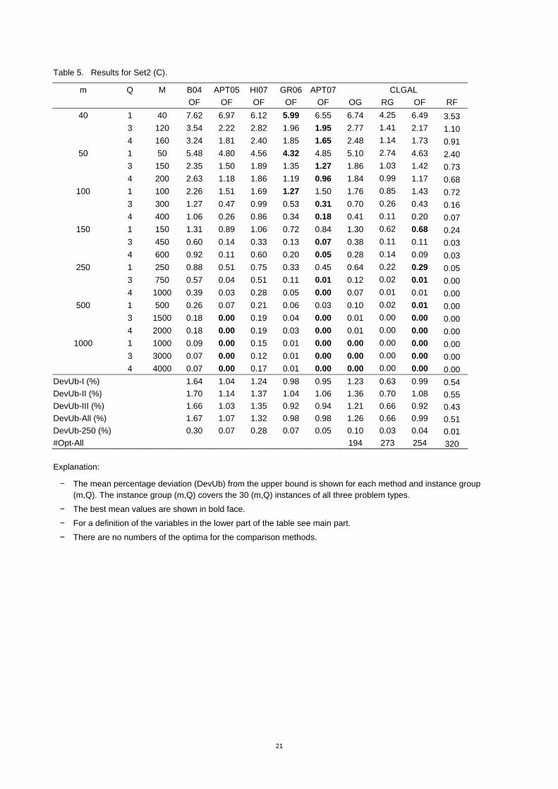
DevUb-I (%) 1.64 1.04 1.24 0.98 0.95 1.23 0.63 0.99 0.54 DevUb-II (%) 1.70 1.14 1.37 1.04 1.06 1.36 0.70 1.08 0.55 DevUb-III (%) 1.66 1.03 1.35 0.92 0.94 1.21 0.66 0.92 0.43 DevUb-All (%) 1.67 1.07 1.32 0.98 0.98 1.26 0.66 0.99 0.51 DevUb-250 (%) 0.30 0.07 0.28 0.07 0.05 0.10 0.03 0.04 0.01 #Opt-All 194 273 254 320

Explanation:

− The mean percentage deviation (DevUb) from the upper bound is shown for each method and instance group (m,Q). The instance group (m,Q) covers the 30 (m,Q) instances of all three problem types.

− The best mean values are shown in bold face.

− For a definition of the variables in the lower part of the table see main part.

− There are no numbers of the optima for the comparison methods.

22

Table 6. Results for Set2, problem type I (C).

m Q M B04 APT05 HI07 GR06 CLGAL OF OF OF OF OG RG OF RF

40 1 40 6.39 6.02 5.35 5.30 5.77 3.42 5.43 3.40 3 120 4.71 2.79 3.36 2.71 3.56 1.76 3.03 1.40 4 160 2.98 1.96 2.20 1.69 2.38 1.32 1.75 1.12

50 1 50 5.19 4.42 4.27 4.22 4.97 2.58 4.37 2.30 3 150 2.54 1.69 2.20 1.50 1.98 1.13 1.51 0.76 4 200 2.68 1.13 1.34 0.95 1.86 0.82 1.16 0.66

100 1 100 1.98 1.47 1.60 1.32 1.69 0.94 1.53 0.95 3 300 1.21 0.51 0.97 0.62 0.60 0.21 0.46 0.17 4 400 1.13 0.28 1.00 0.36 0.43 0.10 0.23 0.09

150 1 150 1.06 0.68 0.86 0.64 0.89 0.53 0.63 0.35 3 450 0.61 0.10 0.32 0.15 0.34 0.10 0.13 0.05 4 600 1.11 0.15 0.60 0.27 0.43 0.10 0.18 0.06

250 1 250 0.83 0.51 0.74 0.33 0.58 0.13 0.31 0.06 3 750 0.69 0.06 0.46 0.19 0.17 0.02 0.02 0.00 4 1000 0.44 0.05 0.14 0.07 0.08 0.01 0.04 0.01

500 1 500 0.22 0.09 0.17 0.10 0.07 0.01 0.03 0.01 3 1500 0.23 0.00 0.18 0.05 0.01 0.00 0.00 0.00 4 2000 0.18 0.00 0.15 0.05 0.00 0.00 0.00 0.00

1000 1 1000 0.09 0.01 0.07 0.01 0.00 0.00 0.00 0.00 3 3000 0.06 0.00 0.05 0.01 0.00 0.00 0.00 0.00 4 4000 0.04 0.00 0.14 0.02 0.00 0.00 0.00 0.00

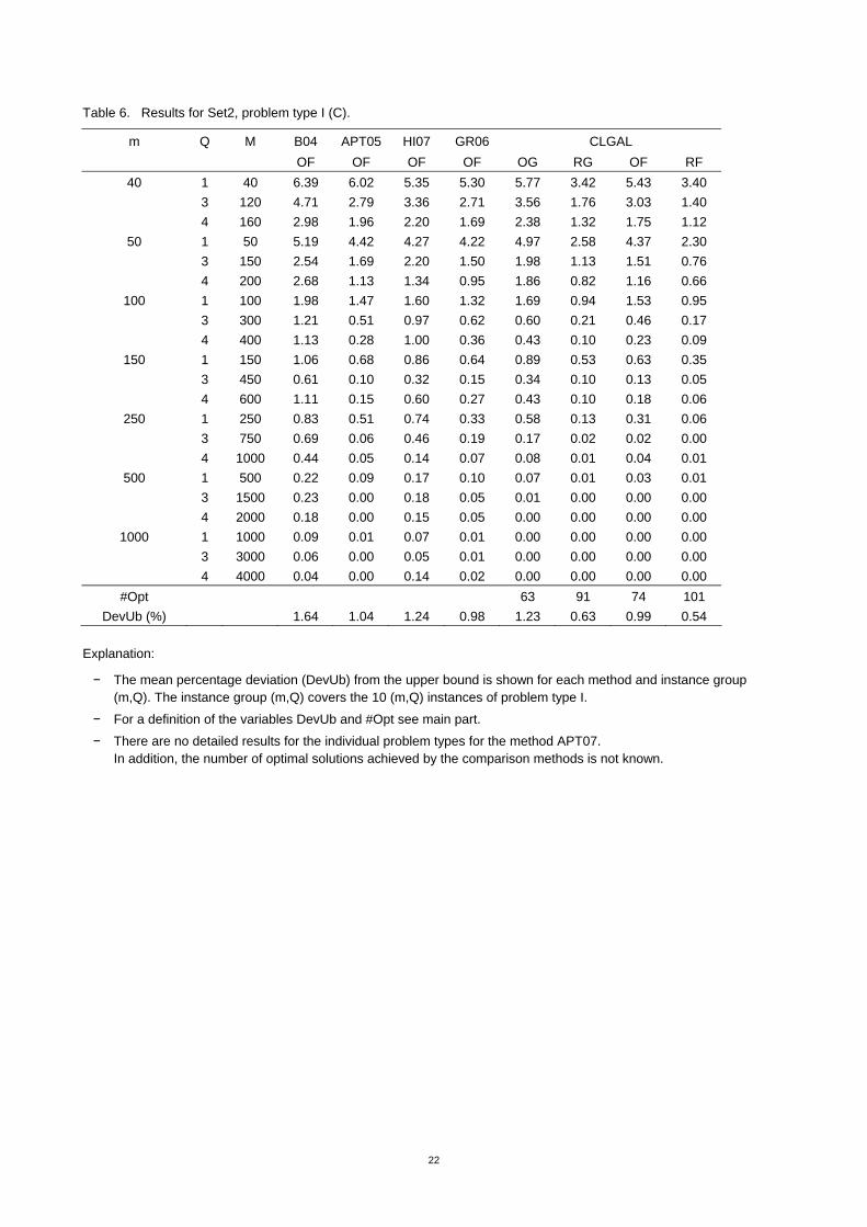
#Opt 63 91 74 101 DevUb (%) 1.64 1.04 1.24 0.98 1.23 0.63 0.99 0.54

Explanation:

− The mean percentage deviation (DevUb) from the upper bound is shown for each method and instance group (m,Q). The instance group (m,Q) covers the 10 (m,Q) instances of problem type I.

− For a definition of the variables DevUb and #Opt see main part.

− There are no detailed results for the individual problem types for the method APT07. In addition, the number of optimal solutions achieved by the comparison methods is not known.

23

Table 7. Results for Set2, problem type II (C).


40 1 40 8.68 8.17 6.91 6.78 8.19 4.64 7.39 3.76 3 120 3.07 2.37 2.93 2.06 2.94 1.41 2.28 1.23 4 160 3.07 2.09 2.77 2.12 2.50 1.26 2.04 0.96

50 1 50 5.97 4.95 4.85 4.40 5.39 3.09 4.89 2.79 3 150 2.12 1.32 1.66 1.29 1.73 0.99 1.43 0.70 4 200 2.78 1.24 2.11 1.34 2.09 1.23 1.31 0.92

100 1 100 2.39 1.48 1.56 1.28 1.78 0.75 1.51 0.69 3 300 1.28 0.42 0.87 0.48 0.82 0.30 0.46 0.16 4 400 1.25 0.35 0.91 0.50 0.64 0.17 0.28 0.07

150 1 150 1.25 0.74 0.86 0.55 1.18 0.39 0.53 0.15 3 450 0.52 0.15 0.34 0.09 0.35 0.10 0.09 0.04 4 600 0.85 0.07 0.57 0.20 0.13 0.12 0.03 0.03

250 1 250 0.95 0.51 0.76 0.37 0.51 0.18 0.32 0.05 3 750 0.44 0.04 0.31 0.09 0.10 0.02 0.01 0.00 4 1000 0.29 0.03 0.38 0.06 0.08 0.01 0.00 0.00

500 1 500 0.28 0.05 0.25 0.07 0.06 0.01 0.00 0.00 3 1500 0.12 0.00 0.11 0.05 0.01 0.01 0.00 0.00 4 2000 0.14 0.00 0.17 0.03 0.02 0.00 0.00 0.00

1000 1 1000 0.09 0.01 0.21 0.01 0.00 0.00 0.00 0.00 3 3000 0.04 0.00 0.08 0.00 0.00 0.00 0.00 0.00 4 4000 0.08 0.00 0.08 0.00 0.00 0.00 0.00 0.00

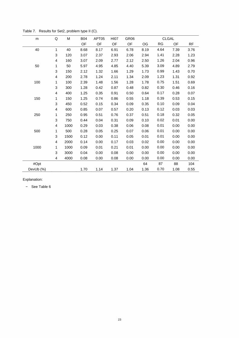
#Opt 64 87 88 104 DevUb (%) 1.70 1.14 1.37 1.04 1.36 0.70 1.08 0.55

Explanation:

− See Table 6

24

Table 8. Results for Set2, problem type III (C).


40 1 40 7.79 6.72 6.11 5.88 6.25 4.68 6.66 3.44 3 120 2.85 1.50 2.17 1.12 1.81 1.06 1.21 0.68 4 160 3.66 1.39 2.22 1.74 2.55 0.85 1.41 0.65

50 1 50 5.28 5.04 4.58 4.35 4.94 2.56 4.64 2.10 3 150 2.39 1.50 1.82 1.26 1.88 0.98 1.28 0.74 4 200 2.42 1.18 2.13 1.29 1.57 0.93 1.05 0.46

100 1 100 2.42 1.58 1.90 1.20 1.81 0.86 1.25 0.51 3 300 1.31 0.49 1.14 0.48 0.69 0.26 0.38 0.14 4 400 0.80 0.16 0.66 0.17 0.16 0.07 0.10 0.04

150 1 150 1.61 1.25 1.45 0.99 1.83 0.94 0.87 0.23 3 450 0.67 0.16 0.32 0.17 0.45 0.13 0.10 0.01 4 600 0.81 0.10 0.62 0.14 0.28 0.20 0.05 0.01

250 1 250 0.86 0.51 0.74 0.31 0.83 0.35 0.23 0.05 3 750 0.59 0.01 0.76 0.05 0.08 0.02 0.00 0.00 4 1000 0.43 0.00 0.33 0.03 0.04 0.01 0.00 0.00

500 1 500 0.29 0.07 0.21 0.02 0.17 0.04 0.00 0.00 3 1500 0.20 0.00 0.28 0.03 0.01 0.00 0.00 0.00 4 2000 0.21 0.00 0.25 0.01 0.00 0.00 0.00 0.00

1000 1 1000 0.09 0.00 0.19 0.01 0.00 0.00 0.00 0.00 3 3000 0.10 0.00 0.22 0.02 0.00 0.00 0.00 0.00 4 4000 0.09 0.00 0.29 0.01 0.00 0.00 0.00 0.00

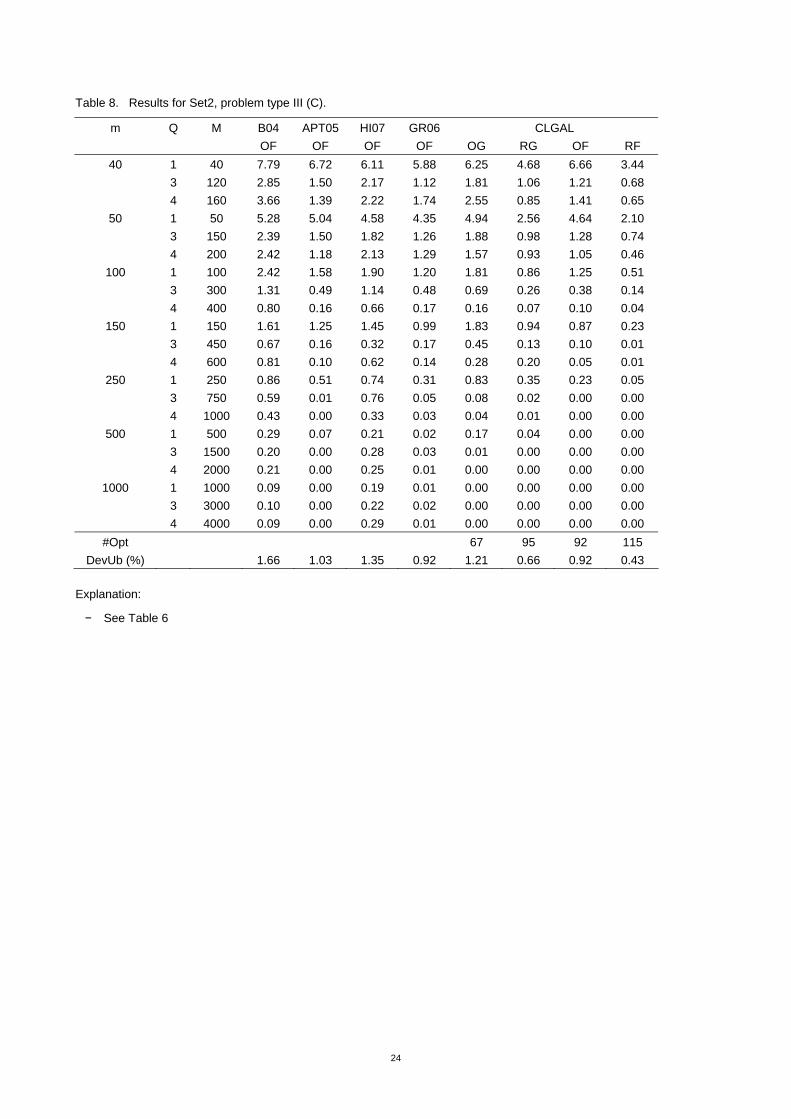
#Opt 67 95 92 115 DevUb (%) 1.66 1.03 1.35 0.92 1.21 0.66 0.92 0.43

Explanation:

− See Table 6

25


Instance Container m M Optimum APT05 GR06 APT07 CLGAL (L,W) OF OF OF OG RG OF RF LC1 (400,200) 9 10 80000 80000 80000 80000 76000 80000 80000 80000 LC2 (400,200) 7 15 79000 79000 79000 79000 79000 79000 79000 79000 LC3 (400,400) 5 20 160000 154600 160000 160000 154600 155200 157300 154600 J1 (70,80) 14 20 5600 5447 5600 5600 5400 5447 5600 5447 J2 (70,80) 16 25 5540 5455 5540 5540 5368 5464 5512 5540 J3 (120,45) 22 25 5400 5328 5400 5400 5400 5400 5400 5400 J4 (90,45) 16 30 4050 3978 4050 4050 3978 4050 4050 4050 J5 (65,45) 18 30 2925 2871 2925 2925 2925 2925 2925 2925 LYT1 (150,110) 40 40 16500 15856 16172 16280 16084 16356 16196 16444 LYT2 (160,120) 50 50 19200 18628 18860 19044 18840 19104 18908 19104 DevOpt (%) 1.95 0.38 0.21 2.12 0.85 0.56 0.69 #Opt 3 8 8 3 5 6 6

Explanation:

− The (best) packed area is shown per method and instance.

− Optimal values are shown in bold face.

− For the variables DevOpt and #Opt see main part.

26


Instance Container m M Optimum APT05 APT07 CLGAL (L,W) OF OF OG RG OF RF

1-1 (20,20) 16 16 400 400 400 400 400 400 400 1-2 (20,20) 17 17 400 386 400 373 396 396 400 1-3 (20,20) 16 16 400 400 400 400 400 400 400 2-1 (40,15) 25 25 600 590 600 600 600 600 600 2-2 (40,15) 25 25 600 597 600 594 600 597 600 2-3 (40,15) 25 25 600 600 600 600 600 600 600 3-1 (60,30) 28 28 1800 1765 1800 1788 1800 1800 1800 3-2 (60,30) 20 20 1800 1755 1800 1756 1796 1781 1800 3-3 (60,30) 28 28 1800 1774 1800 1800 1800 1800 1800 4-1 (60,60) 49 49 3600 3528 3580 3530 3600 3576 3600 4-2 (60,60) 49 49 3600 3524 3564 3551 3596 3582 3600 4-3 (60,60) 49 49 3600 3544 3580 3570 3600 3586 3600 5-1 (60,90) 73 73 5400 5308 5342 5351 5400 5388 5400 5-2 (60,90) 73 73 5400 5313 5361 5326 5400 5386 5400 5-3 (60,90) 73 73 5400 5312 5375 5368 5400 5382 5400 6-1 (80,120) 97 97 9600 9470 9548 9506 9588 9555 9588 6-2 (80,120) 97 97 9600 9453 9448 9521 9600 9575 9600 6-3 (80,120) 97 97 9600 9450 9565 9518 9594 9568 9600 7-1 (160,240) 196 196 38400 37661 38026 38083 38337 38005 38328 7-2 (160,240) 197 197 38400 37939 38145 38171 38394 38157 38385 7-3 (160,240) 196 196 38400 37745 37867 38061 38379 38127 38342

DevOpt (%) 1.50 0.47 1.09 0.08 0.40 0.02 #Opt 3 9 5 13 6 17 #Best 3 10 7 15

Explanation:

− The (best) packed area is shown per method and instance.

− Optimal values are shown in bold face, best values with regard to subtypes OF and OG are shown in italics.

− For the variables DevOpt, #Opt and #Best see main part.

27


Instance Container m Optimum FHZ98 APT02 MP07 CLGAL (L,W) (OG) OG OG OG OG RG

CU1 (100,125) 25 12330 12312 12330 12330 12330 12352 CU2 (150,175) 35 26100 25806 26100 26100 26100 26200 CU3 (134,125) 45 16723 16608 16679 16723 16598 16723 CU4 (285,354) 45 99945 98190 99366 99945 98764 99888 CU5 (456,385) 50 173364 171651 173364 173364 171935 174057 CU6 (356,447) 45 158572 158572 158572 158572 158572 158572 CU7 (563,458) 45 247150 246860 247150 247150 246143 252318 CU8 (587,756) 35 433331 432198 432714 433331 431126 438383 CU9 (856,785) 25 657055 657055 657055 657055 657055 657828 CU10 (794,985) 40 773772 764696 773485 773772 772118 776369 CU11 (977,953) 50 924696 913387 922161 924696 918304 922576 CW1 (125,105) 25 6402 6402 6402 6402 6402 6746 CW2 (145,165) 35 5354 5354 5354 5354 5354 5548 CW3 (267,207) 40 5689 5148 5689 5689 5689 5744 CW4 (465,387) 39 6175 6168 6170 6175 6175 7496 CW5 (524,678) 35 11659 11550 11644 11659 11644 11659 CW6 (781,657) 55 12923 12403 12923 12923 12923 13011 CW7 (376,374) 45 9898 9484 9898 9898 9425 9636 CW8 (305,287) 60 4605 4504 4605 4605 4504 4736 CW9 (405,362) 50 10748 10748 10748 10748 10748 11479 CW10 (992,970) 60 6515 6116 6515 6515 6134 6306 CW11 (982,967) 60 6321 6084 6321 6321 5940 6188

DevOpt (%) 1.74 0.07 0.00 1.07 -1.73 #Opt 5 15 22 10

Explanation:

− The (best) packed area (CU1-CU11) or the (best) packed value (CW1-CW11) is shown per method and instance.



− See the corresponding notes on Table 4 with regard to column CLGAL-RG.

28

Table 12. Results for Set6 (UC).

Instance Container m Optimum FHZ98 CLGAL (L,W) OG OG

UU1 (500,500) 25 242919 241260 232481UU2 (750,800) 30 595288 595288 582342UU3 (1100,1000) 25 1072764 1072764 1056682UU4 (1000,1200) 38 1179050 1178295 1170000UU5 (1450,1300) 50 1868999 1868985 1866789UU6 (2050,1457) 38 2950760 2950760 2883383UU7 (1465,2024) 50 2930654 2930654 2900654UU8 (2000,2000) 55 3959352 3959352 3929352UU9 (2500,2460) 60 6100692 6100692 6027616UU10 (3500,3450) 55 11955852 11955852 11749280UU11 (3500,3765) 25 13157811 13141175 13060336UW1 (500,500) 25 6036 6036 6036UW2 (560,750) 35 8468 8468 8160UW3 (700,650) 35 6302 6226 5964UW4 (1245,1015) 45 8326 8326 7748UW5 (1100,1450) 34 7780 7780 7780UW6 (1750,1542) 47 6615 6615 5976UW7 (2250,1875) 50 10464 10464 10464UW8 (2645,2763) 55 7692 7692 7692UW9 (3000,3250) 45 7038 7038 7038UW10 (3500,3650) 60 7507 7507 7507UW11 (555,632) 25 15747 15747 15747

DevOpt(%) 0.09 1.92#Opt 17 7

Explanation:

− The (best) packed area (UU1-UU11) or the (best) packed value (UW1-UW11) is shown per method and instance.



a genetic algorithm for the two-dimensional knapsack ... · the 2d knapsack problem is np hard (cf....

Documents