A New Asymptotic Theory for Heteroskedasticity-AutocorrelationRobust Tests

Nicholas M. Kiefer and Timothy J. Vogelsang�

Departments of Economics and Statistical Science, Cornell University

April 2002, Revised March 23, 2005

Abstract

A new �rst-order asymptotic theory for heteroskedasticity-autocorrelation (HAC) robusttests based on nonparametric covariance matrix estimators is developed. The bandwidth of thecovariance matrix estimator is modeled as a �xed proportion of the sample size. This leadsto a distribution theory for HAC robust tests that explicitly captures the choice of bandwidthand kernel. This contrasts with the traditional asymptotics (where the bandwidth increasesslower than the sample size) where the asymptotic distributions of HAC robust tests do notdepend on the bandwidth or kernel. Finite sample simulations show that the new approach ismore accurate than the traditional asymptotics. The impact of bandwidth and kernel choiceon size and power of t-tests is analyzed. Smaller bandwidths lead to tests with higher powerbut greater size distortions and large bandwidths lead to tests with lower power but less sizedistortions. Size distortions across bandwidths increase as the serial correlation in the databecomes stronger. Overall, the results clearly indicate that for bandwidth and kernel choicethere is a trade-o¤ between size distortions and power. Finite sample performance using thenew asymptotics is comparable to the bootstrap which suggests the asymptotic theory in thispaper could be useful in understanding the theoretical properties of the bootstrap when appliedto HAC robust tests.

Keywords: Covariance matrix estimator, inference, autocorrelation, truncation lag, prewhiten-ing, generalized method of moments, functional central limit theorem, bootstrap.

�We thank an editor and a referee for constructive comments on a previous version of the paper. Helpful commentsprovided by Cli¤ Hurvich, Andy Levin, Je¤ Simono¤ and seminar participants at NYU (Statistics), U. Texas Austin,Yale, U. Montreal, UCSD, UC Riverside, UC Berkeley, U. of Pittsburgh, SUNY Albany, U. Aarhus, Brown U.,NBER/NSF Time Series Conference and 2003 Winter Meetings of the Econometrics Society are gratefully acknowl-edge. We gratefully acknowledge �nancial support from the National Science Foundation through grant SES-0095211.We thank the Center for Analytic Economics at Cornell University. Corresponding Author: Tim Vogelsang, Depart-ment of Economics, Uris Hall, Cornell University, Ithaca, NY 14853-7601, Phone: 607-255-5108, Fax: 607-255-2818,email: tjv2@cornell.edu

1 Introduction

We provide a new and improved approach to the asymptotics of hypothesis testing in time series

models with �arbitrary,� i.e. unspeci�ed, serial correlation and heteroskedasticity. Our results

are general enough to apply to stationary models estimated by generalized method of moments

(GMM). Heteroskedasticity and autocorrelation consistent (HAC) estimation and testing in these

models involves calculating an estimate of the spectral density at zero frequency of the estimating

equations or moment conditions de�ning the estimator. We focus on the class of nonparametric

spectral density estimators1 which were originally proposed and analyzed in the time series statistics

literature. See Priestley (1981) for the standard textbook treatment. Important contributions

to the development of these estimators for covariance matrix estimation in econometrics include

White (1984), Newey and West (1987), Gallant (1987), Gallant and White (1988), Andrews (1991),

Andrews and Monahan (1992), Hansen (1992), Robinson (1998), de Jong and Davidson (2000) and

Jansson (2002).

We stress at the outset that we are not proposing new estimators or statistics; rather we focus

on improving the asymptotic distribution theory for existing techniques. Our results provide a

framework that can be used assess the impact of the choice of HAC estimator on the resulting test

statistic.

Conventional asymptotic theory for HAC estimators is well established and has proved useful

in providing practical formulas for estimating asymptotic variances. The ingenious �trick� is the

assumption that the variance estimator depends on a fraction of sample autocovariances, with

the number of sample autocovariances going to in�nity, but the fraction going to zero as the

sample size grows. Under this condition it has been shown that well-known HAC estimators of the

asymptotic variance are consistent. Then, the asymptotic distribution of estimated coe¢ cients can

essentially be derived assuming the variance is known. That is, sampling bias and variance of the

variance estimator does not appear in the �rst-order asymptotic distribution theory of test statistics

regarding parameters of interest. While this is an extremely productive simplifying assumption that

leads to standard asymptotic distribution theory for tests, the accuracy of the resulting asymptotic

theory is often less than satisfactory. In particular there is a tendency for HAC robust tests to over

reject (sometimes substantially) under the null hypothesis in �nite samples; see Andrews (1991),

Andrews and Monahan (1992), and the July 1996 special issue of Journal of Business and Economic

Statistics for evidence.

There are two main sources of �nite sample distortions. The �rst source is inaccuracy via the

central limit theorem approximation to the sampling distribution of parameters of interest. This

becomes a serious problem for data that has strong or persistent serial correlation. The second

source is the bias and sampling variability of the HAC estimate of the asymptotic variance. This

1

second source is the focus of this paper. Simply appealing to a consistency result for the asymptotic

variance estimator as is done under the standard approach does not capture these important small

sample properties.

The assumption that the fraction of the sample autocovariances used in calculating the HAC

variance estimator goes to zero as the sample size goes to in�nity is a clever technical assumption

that substantially simpli�es asymptotic calculations. However, in practice there is a given sample

size and some fraction of sample autocovariances is used to estimate the asymptotic variance. Even

if a practitioner chooses the fraction based on a rule such that the fraction goes to zero as the

sample size grows, it does not change the fact that a positive fraction is being used for a particular

data set. The implications of this simple observation have been eloquently summarized by Neave

(1970, p.70) in the context of spectral density estimation:

�When proving results on the asymptotic behavior of estimates of the spectrum of a

stationary time series, it is invariably assumed that as the sample size T tends to in�nity,

so does the truncation point M , but at a slower rate, so that M=T tends to zero. This

is a convenient assumption mathematically in that, in particular, it ensures consistency

of the estimates, but it is unrealistic when such results are used as approximations to

the �nite case where the value of M=T cannot be zero�.

Based on this observation, Neave (1970) derived an asymptotic approximation for the sampling

variance of spectral density estimates under the assumption that M=T is a constant and showed

that his approximation was more accurate than the standard approximation.

In this paper, we e¤ectively generalize the approach of Neave (1970) for zero frequency nonpara-

metric spectral density estimators (HAC estimators). We derive the entire asymptotic distribution

(rather than just the variance) of these estimators under the assumption that M = bT where

b 2 (0; 1] is a constant. We label asymptotics obtained under this nesting of the bandwidth,

��xed-b asymptotics�. In contrast, under the standard asymptotics b goes to zero as T increases.

Therefore, we refer to the standard asymptotics as �small-b asymptotics�. We show that under

�xed-b asymptotics, the HAC robust variance estimators converge to a limiting random matrix that

is proportional to the unknown asymptotic variance and has a limiting distribution that depends

on the kernel and b. Under the �xed-b asymptotics, HAC robust test statistics computed in the

usual way are shown to have limiting distributions that are pivotal but depend on the kernel and

b. This contrasts with small-b asymptotics where the e¤ects of the kernel and bandwidth are not

captured.

Fixed-b asymptotics is a natural generalization of ideas explored by Kiefer, Vogelsang and

Bunzel (2000), Bunzel, Kiefer and Vogelsang (2001), Kiefer and Vogelsang (2002a), Kiefer and

Vogelsang (2002b) and Vogelsang (2003). Those papers analyzed HAC robust tests for the case

2

where the HAC bandwidth is set equal to the sample size, i.e. b = 1. By considering values of b < 1

in this paper, we follow the traditional approach where the bandwidth controls the downweighting

on higher order sample autocovariances. An alternative has been proposed in recent work by

Phillips, Sun and Jin (2003) and Phillips, Sun and Jin (2005) where downweighting is achieved by

exponentiating kernels that use bandwidth equal to the sample size. They show that if the exponent

increases with the sample size at a suitable rate, then consistent and asymptotically normal HAC

variance estimators can be obtained. In an analysis analogous to �xed-b asymptotics, they also

develop an asymptotic theory under the assumption that the exponent is �xed as the sample size

increases. Fixed-exponent asymptotics captures the choice of kernel and exponent in much the

same way that �xed-b asymptotics captures the choice of kernel and bandwidth.

While the �xed-b assumption is a better re�ection of practice in reality, that alone does not

justify the new asymptotic theory. In fact, our asymptotic theory leads to two important innovations

for HAC robust testing.

First, because the �xed-b asymptotics explicitly captures the choice of bandwidth and kernel, a

more accurate �rst-order asymptotic approximation is obtained for HAC robust tests. Finite sample

simulations reported here and in the working paper, Kiefer and Vogelsang (2002c), show that in

many situations the �xed-b asymptotics provide a more accurate approximation than the standard

small-b asymptotics. There is also theoretical evidence by Jansson (2004) showing that �xed-b

asymptotics is more accurate than small-b asymptotics in Gaussian location models for the special

case of the Bartlett kernel with b = 1. Jansson (2004) proves that �xed-b asymptotics delivers an

error in rejection probability that is O(T�1 log(T )). This contrasts with small-b asymptotics where

the error in rejection probability is no smaller than O(T�1=2) (see Velasco and Robinson (2001)).

Again focusing on Gaussian location models, recent work by Phillips, Sun and Jin (2004) has shown

that the error in rejection probability is O(T�1) for exponentiated kernels under �xed-exponent

asymptotics. Phillips et al. (2004) conjecture that this result likely extends to traditional kernels

under �xed-b asymptotics. If this conjecture is true, then �xed-b asymptotics has an error in

rejection probability of smaller order than the standard normal approximation (small-b).

Second, �xed-b asymptotic theory permits a local asymptotic power analysis for HAC robust

tests that depends on the kernel and bandwidth. We can theoretically analyze how the choices of

kernel and bandwidth a¤ect the power of HAC robust tests. Such an analysis is not possible under

the standard small-b asymptotics because local asymptotic power does not depend on the choice of

kernel or bandwidth. Because of this fact, the existing HAC robust testing literature has focused

instead on minimizing the asymptotic truncated MSE of the asymptotic variance estimators when

choosing the kernel and bandwidth. For the analysis of HAC robust tests, this is not a completely

satisfying situation as noted by Andrews (1991, p.828)2.

An obvious alternative to asymptotic approximations is the bootstrap. Recently it has been

3

shown by Hall and Horowitz (1996), Götze and Künsch (1996), Inoue and Shintani (2004) and

others that higher order re�nements to the small-b asymptotics are feasible when bootstrapping

the distribution of HAC robust tests using blocking. Using �nite sample simulations we compare

�xed-b asymptotics with the block bootstrap. Our results suggest some interesting properties of the

bootstrap and indicate that �xed-b asymptotics may be a useful analytical tool for understanding

variation in bootstrap performance across bandwidths. One result is that the bootstrap without

blocking performs almost identically to the �xed-b asymptotics even when the data are dependent

(in contrast the small-b asymptotics performs relatively poorly). When blocking is used, the boot-

strap can perform slightly better or slightly worse than �xed-b asymptotics depending on the choice

of block length. It may be the case that the block bootstrap delivers an asymptotic re�nement over

the �xed-b �rst-order asymptotics if the block length is chosen in a suitable way. A higher order

�xed-b asymptotic theory is required before such a result can be formally established.

The remainder of the paper is organized as follows. Section 2 lays out the GMM framework and

reviews standard results. Section 3 reports some small sample simulation results that illustrate the

inaccuracies that can occur when using the small-b asymptotic approximation. Section 4 introduces

the new �xed-b asymptotic theory. Section 5 analyzes the performance of the new asymptotic theory

in terms of size distortions and local asymptotic power. The impact of the choice of bandwidth

and kernel is analyzed and comparisons are made with the traditional small-b asymptotics and the

block bootstrap. Section 6 gives concluding comments. Proofs are provided in an appendix.

The following notation is used throughout the paper. The symbol) denotes weak convergence,

Bj(r) denotes a j vector of standard Brownian motions (Wiener processes) de�ned on r 2 [0; 1],eBj(r) = Bj(r) � rBj(1) denotes a j vector of standard Brownian bridges, and [rT ] denotes theinteger part of rT for r 2 [0; 1].

2 Inference in GMM Models: The Standard Approach

We present our results in the GMM framework noting that this covers estimating equation methods

(Heyde, 1997). Since the in�uential work of Hansen (1982), GMM is widely used in virtually every

�eld of economics. Heteroskedasticity or autocorrelation of unknown form is often an important

speci�cation issue especially in macroeconomics and �nancial applications. Typically the form of

the correlation structure is not of direct interest (if it is, it should be modeled directly). What

is desired is an inference procedure that is robust to the form of the heteroskedasticity and serial

correlation. HAC covariance matrix estimators were developed for exactly this setting.

Consider the p � 1 vector of parameters, � 2 � � Rp. Let �0 denote the true value of �, andassume �0 is an interior point of �. Let vt denote a vector of observed data and assume that q

4

moment conditions hold that can be written as

E[f(vt; �0)] = 0; t = 1; 2; :::; T; (1)

where f(�) is a q � 1 vector of functions with q � p and rank(E [@f=@�0]) = p. The expectation

is taken over the endogenous variables in vt, and may be conditional on exogenous elements of vt.

There is no need in what follows to make this conditioning explicit in the notation. De�ne

gt(�) = T�1

tXj=1

f(vj ; �);

where gT (�) = T�1PTt=1 f(vt; �) is the sample analog to (1). The GMM estimator is de�ned as

b�T = argmin�2�

gT (�)0WT gT (�) (2)

where WT is a q � q positive de�nite weighting matrix. Alternatively, b�T can also be de�ned as anestimating equations estimator, the solution to the p �rst-order conditions associated with (2)

GT (b�T )0WT gT (b�T ) = 0; (3)

where Gt(�) = T�1Ptj=1 @f(vj ; �)=@�

0. Of course, when the model is exactly identi�ed and q = p,

an exact solution to gT (b�T ) = 0 is attainable and the weighting matrixWT is irrelevant. Application

of the mean-value theorem implies that

gt(b�T ) = gt(�0) +Gt(b�T ; �0; �T )(b�T � �0) (4)

where Gt(b�T ; �0; �T ) denotes the q � p matrix whose ith row is the corresponding row of Gt(�(i)T )where �

(i)T = �i;T �0+(1��i;T )b�T for some 0 � �i;T � 1 and �T is the q� 1 vector with ith element

�i;T .

In order to focus on the new asymptotic theory for tests, we avoid listing primitive assumptions

and make rather high-level assumptions on the GMM estimator b�T . Lists of su¢ cient conditions forthese to hold can be found in Hansen (1982) and Newey and McFadden (1994). Our assumptions

are:

Assumption 1 p lim b�T = �0:Assumption 2 T�1=2

P[rT ]t=1 f(vt; �0) = T 1=2g[rT ](�0) ) �Bq(r) where ��0 = =

P1j=�1 �j ;

�j = E[f(vt; �0)f(vt�j ; �0)0].

Assumption 3 p limG[rT ](b�T ) = rG0 and p limG[rT ](b�T ; �0; �T ) = rG0 uniformly in r 2 [0; 1]

where G0 = E[@f(vt; �0)=@�0].

5

Assumption 4 WT is positive semi-de�nite and p limWT = W1 where W1 is a matrix of con-

stants and G00W1G0 is positive de�nite.

These assumptions hold for many models in economics, and with the exception of Assumption

2 they are fairly standard. Assumption 2 requires that a functional central limit theorem hold

for T 1=2gt(�0). This is stronger than the central limit theorem for T 1=2gT (�0) that is required

for asymptotic normality of b�T . However, consistent estimation of the asymptotic variance of b�Trequires an estimate of . Conditions for consistent estimation of are typically stronger than

Assumption 2 and often imply Assumption 2. For example, Andrews (1991) requires that f(vt; �0)

is a mean zero fourth order stationary process that is � � mixing. Phillips and Durlauf (1986)show that Assumption 2 holds under the weaker assumption that f(vt; �0) is a mean zero, 2 + �

order stationary process (for some � > 0) that is � �mixing: Thus our assumptions are slightlyweaker than those usually given for asymptotic testing in HAC-estimated GMM models.

Under our assumptions b�T is asymptotically normally distributed, as recorded in the followinglemma which is proved in the appendix.

Lemma 1 Under Assumptions 1 - 4, as T !1,

T 1=2(b�T � �0)) �(G00W1G0)�1��Bp(1) � N(0; V );

where ����0 = G00W1��0W1G0 and V = (G00W1G0)�1����0(G00W1G0)�1:

Under the standard approach, a consistent estimator of V is required for inference. Let b denotean estimator of . Then V can be estimated by

bV = [GT (b�T )0WTGT (b�T )]�1GT (b�T )0WTbWTGT (b�T )[GT (b�T )0WTGT (b�T )]�1: (5)

The HAC literature builds on the spectral density estimation literature to suggest feasible

estimators of and to �nd conditions under which such estimators are consistent. The widely used

class of nonparametric estimators of take the form

b = T�1Xj=�(T�1)

k(j=M)b�j (6)

with b�j = T�1 TXt=j+1

f(vt; b�T )f(vt�j ; b�T )0 for j � 0; b�j = b�0�j for j < 0;where k(x) is a kernel function k : R ! R satisfying k(x) = k(�x), k(0) = 1, jk(x)j � 1, k(x)

continuous at x = 0 andR1�1 k

2(x)dx < 1. Often k(x) = 0 for jxj > 1 so M �trims�the sample

autocovariances and acts as a truncation lag. Some popular kernel functions do not truncate, and

6

M is often called a bandwidth parameter in those cases. For kernels that truncate, the cuto¤

at jxj = 1 is arbitrary and is essentially a normalization. For kernels that do not truncate, a

normalization must be made since the weights generated by the kernel k(x) and bandwidth, M are

the same as those generated by kernel k(ax) with bandwidth aM . Therefore, there is an interaction

between bandwidth and kernel choice. We focus on kernels that yield positive de�nite b for theobvious practical reasons although many of our theoretical results hold without this restriction.

Standard asymptotic analysis proceeds under the assumption that M ! 1 and M=T ! 0

as T ! 1 in which case b is a consistent estimator. Thus, b ! 0 as T ! 1 and hence the

label, small-b asymptotics. Because in practical settings b is strictly positive, the assumption that

b shrinks to zero has little to do with econometric practice; rather it is an ingenious technical

assumption allowing an estimable asymptotic approximation to the asymptotic distribution of b�Tto be calculated. The di¢ culty in practice is that any choice ofM for a given sample size, T , can be

made consistent with the above rate requirement. Although the rate requirement can been re�ned

if one is interested in minimizing the MSE of b (e.g. M must increase at rate T 1=3 for the Bartlett

kernel), these re�nements do not deliver speci�c choices for M . This fact has long been recognized

in the spectral density and HAC literatures and data dependent methods for choosing M have

been proposed. See Andrews (1991) and Newey and West (1994). These papers suggest choosing

M to minimize the truncated MSE of b. However, because the MSE of b depends on the serialcorrelation structure of f(vt; �0); the practitioner must estimate the serial correlation structure

of f(vt; �0) either nonparametrically or with an �approximate� parametric model. While data

dependent methods are a signi�cant improvement over the basic case for empirical implementation,

the practitioner is still faced with either a choice of approximating parametric model or the choice

of bandwidth in a preliminary nonparametric estimation problem. Even these bandwidth rules do

not yield unique bandwidth choices in practice because, for example, if a bandwidth, MA satis�es

the optimality criterion of Andrews (1991), then the bandwidth,MA+d where d is a �nite constant

is also optimal. See den Haan and Levin (1997) for details and additional practical challenges.

As the previous discussion makes clear, the standard approach addresses the choice of bandwidth

by determining the rate by which M must grow to deliver a consistent variance estimator so that

the usual standard normal approximation can be justi�ed. In contrast, for a given data set and

sample size, we take the choice of M as given and provide an asymptotic theory that re�ects to

some extent how that choice of M a¤ects the sampling distribution of the HAC robust test.

3 Motivation: Finite Sample Performance of Standard Asymptotics

While the poor �nite sample performance of HAC robust test in the presence of strong serial

correlation is well documented, it will be useful for later comparisons to illustrate some of these

problems brie�y in a simple environment. Consider the most basic univariate time series model

7

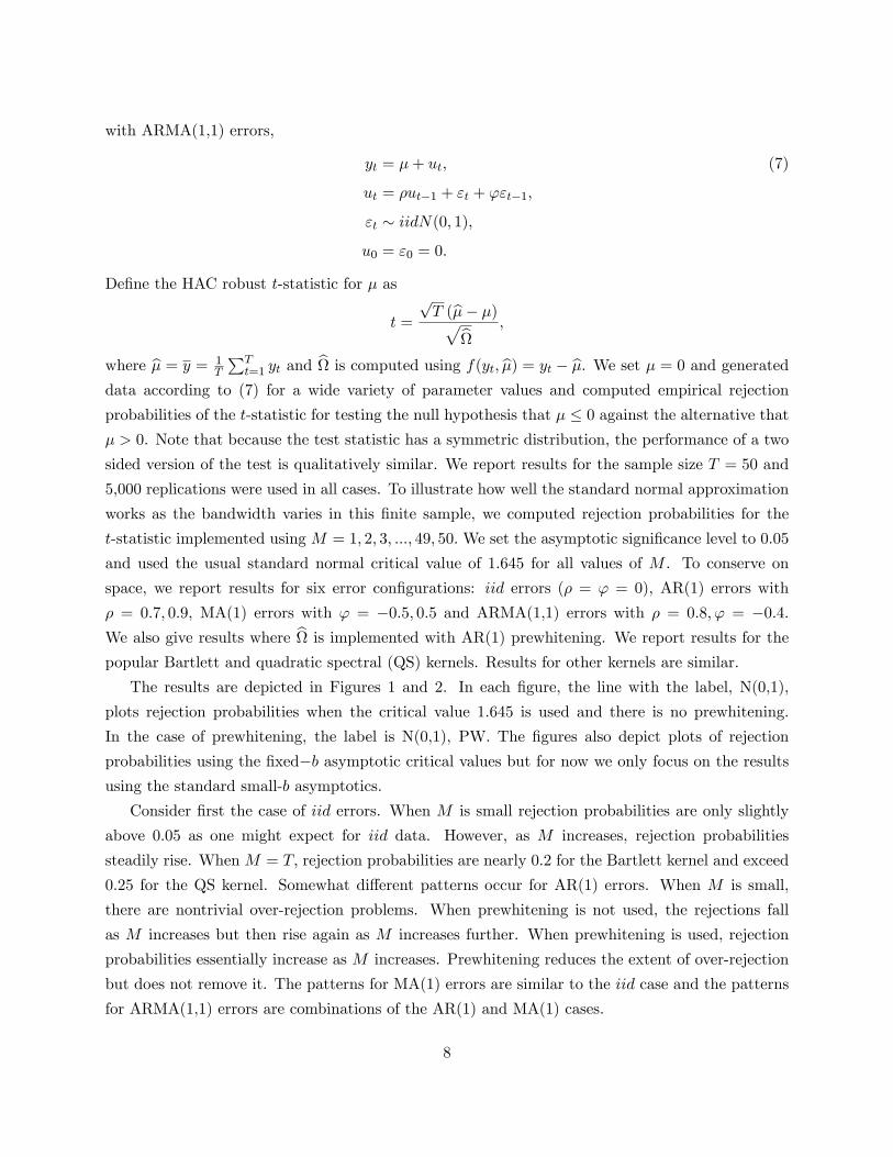
with ARMA(1,1) errors,

yt = �+ ut; (7)

ut = �ut�1 + "t + '"t�1;

"t � iidN(0; 1);

u0 = "0 = 0:

De�ne the HAC robust t-statistic for � as

t =

pT (b�� �)pb ;

where b� = y = 1T

PTt=1 yt and b is computed using f(yt; b�) = yt � b�. We set � = 0 and generated

data according to (7) for a wide variety of parameter values and computed empirical rejection

probabilities of the t-statistic for testing the null hypothesis that � � 0 against the alternative that� > 0. Note that because the test statistic has a symmetric distribution, the performance of a two

sided version of the test is qualitatively similar. We report results for the sample size T = 50 and

5,000 replications were used in all cases. To illustrate how well the standard normal approximation

works as the bandwidth varies in this �nite sample, we computed rejection probabilities for the

t-statistic implemented using M = 1; 2; 3; :::; 49; 50:We set the asymptotic signi�cance level to 0.05

and used the usual standard normal critical value of 1.645 for all values of M . To conserve on

space, we report results for six error con�gurations: iid errors (� = ' = 0), AR(1) errors with

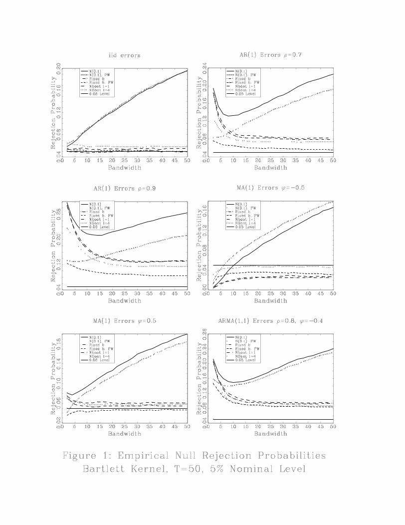
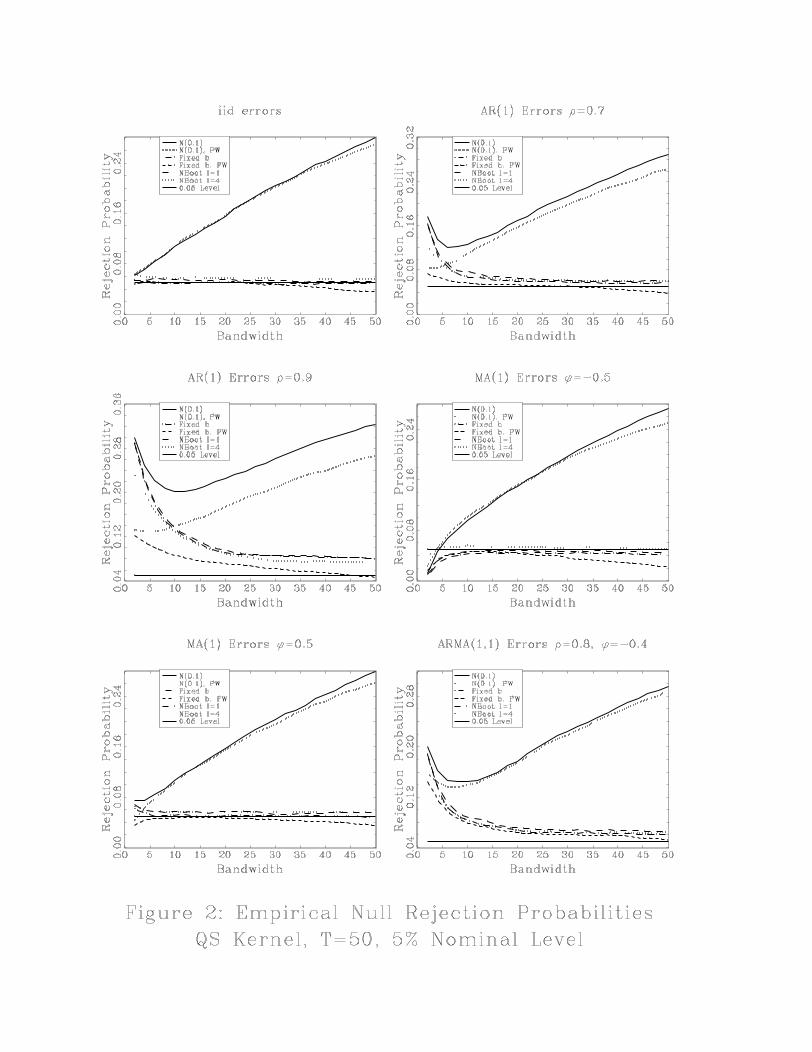
� = 0:7; 0:9, MA(1) errors with ' = �0:5; 0:5 and ARMA(1,1) errors with � = 0:8; ' = �0:4.We also give results where b is implemented with AR(1) prewhitening. We report results for thepopular Bartlett and quadratic spectral (QS) kernels. Results for other kernels are similar.

The results are depicted in Figures 1 and 2. In each �gure, the line with the label, N(0,1),

plots rejection probabilities when the critical value 1.645 is used and there is no prewhitening.

In the case of prewhitening, the label is N(0,1), PW. The �gures also depict plots of rejection

probabilities using the �xed�b asymptotic critical values but for now we only focus on the resultsusing the standard small-b asymptotics.

Consider �rst the case of iid errors. When M is small rejection probabilities are only slightly

above 0.05 as one might expect for iid data. However, as M increases, rejection probabilities

steadily rise. WhenM = T; rejection probabilities are nearly 0.2 for the Bartlett kernel and exceed

0.25 for the QS kernel. Somewhat di¤erent patterns occur for AR(1) errors. When M is small,

there are nontrivial over-rejection problems. When prewhitening is not used, the rejections fall

as M increases but then rise again as M increases further. When prewhitening is used, rejection

probabilities essentially increase as M increases. Prewhitening reduces the extent of over-rejection

but does not remove it. The patterns for MA(1) errors are similar to the iid case and the patterns

for ARMA(1,1) errors are combinations of the AR(1) and MA(1) cases.

8

These plots clearly illustrate a fundamental �nite sample property of HAC robust tests: the

choice ofM in a given sample matters and can greatly a¤ect the extent of size distortion depending

on the serial correlation structure of the data. And, when M is not very small, the choice of

kernel also matters for the over-rejection problem. Given that the sampling distribution of the

test depends on the bandwidth and kernel, it would seem to be a minimal requirement that the

asymptotic approximation re�ect this dependence. Whereas the standard small-b asymptotics is too

crude for this purpose, our results in the next section show that the �xed-b asymptotics naturally

captures the dependence on the bandwidth and kernel and captures the dependence in a simple

and elegant manner3.

Before moving on, it is useful to discuss in some detail the reason that rejection probabilities have

the non-monotonic pattern for AR(1) errors. WhenM is small, b is biased but has relatively smallvariance. Because the bias is downward, that leads to over-rejection. As M initially increases, bias

falls and variance rises. The bias e¤ect is more important for over-rejection (see Simono¤ (1993))

and the extent of over-rejection decreases. According to the conventional, but wrong, wisdom, the

story would be that as M increases further bias continues to fall but variance increases so much

that over-rejections become worse4. This is not what is happening. In fact, as M increases further,

bias eventually increases and variance falls. It is the increase in bias that leads to the large over-

rejections when M is large. The reason that bias increases and variance shrinks as M gets large is

easy to explain. When M is large, high weights are placed on high order sample autocovariances.

In the extreme case where full weight is placed on all of the sample autocovariances, it is well known

that b = 0, and this occurs because b is computed using residuals that have a sample average ofzero. Obviously, b = 0 it is an estimator with large bias and zero variance. Thus, as M increases,b is pushed closer to the full weight case.4 A New Asymptotic Theory

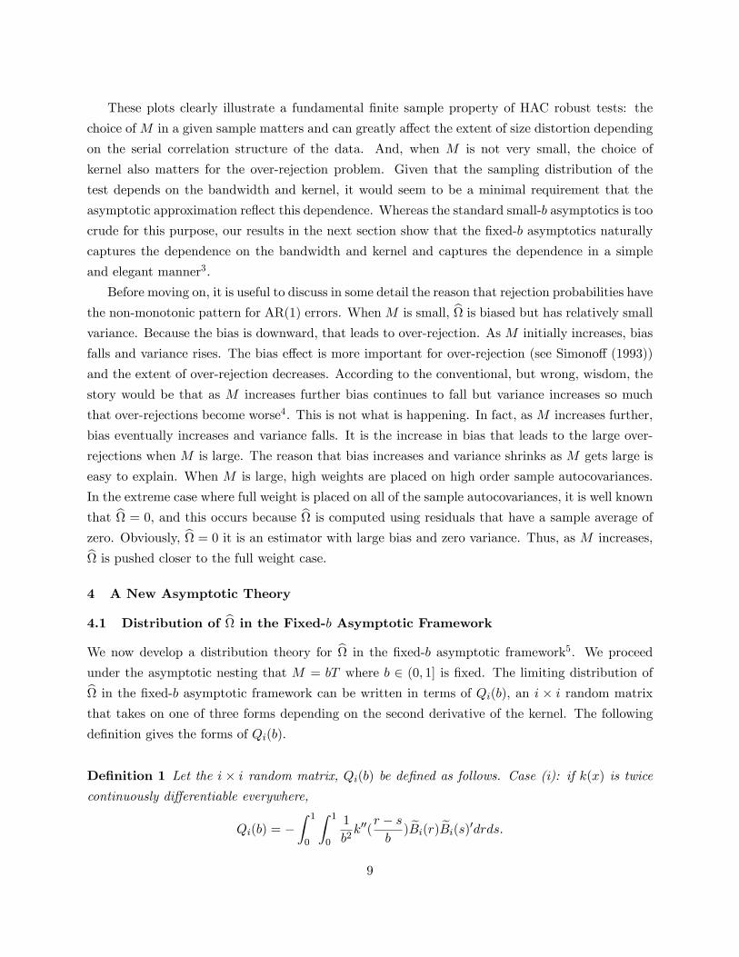
4.1 Distribution of b in the Fixed-b Asymptotic FrameworkWe now develop a distribution theory for b in the �xed-b asymptotic framework5. We proceed

under the asymptotic nesting that M = bT where b 2 (0; 1] is �xed. The limiting distribution ofb in the �xed-b asymptotic framework can be written in terms of Qi(b), an i � i random matrix

that takes on one of three forms depending on the second derivative of the kernel. The following

de�nition gives the forms of Qi(b):

De�nition 1 Let the i � i random matrix, Qi(b) be de�ned as follows. Case (i): if k(x) is twice

continuously di¤erentiable everywhere,

Qi(b) = �Z 1

0

Z 1

0

1

b2k00(

r � sb) eBi(r) eBi(s)0drds:

9

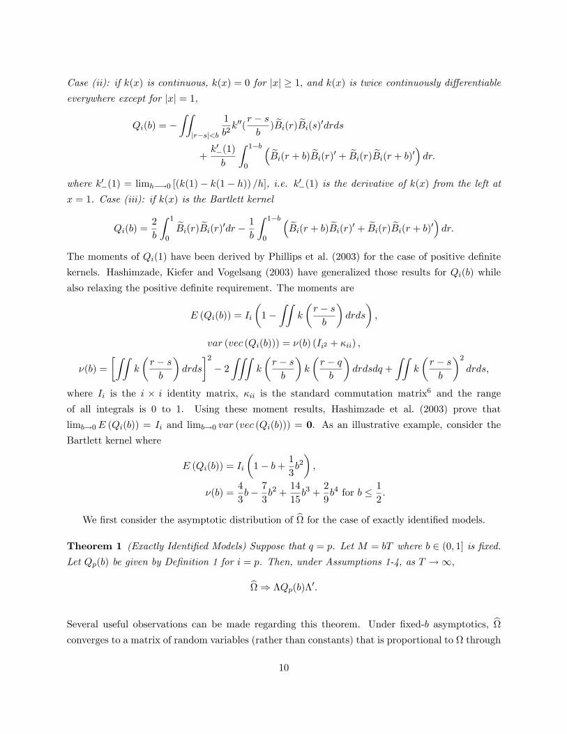
Case (ii): if k(x) is continuous, k(x) = 0 for jxj � 1; and k(x) is twice continuously di¤erentiableeverywhere except for jxj = 1,

Qi(b) = �ZZ

jr�sj<b

1

b2k00(

r � sb) eBi(r) eBi(s)0drds

+k0�(1)

b

Z 1�b

0

� eBi(r + b) eBi(r)0 + eBi(r) eBi(r + b)0� dr:where k0�(1) = limh�!0 [(k(1)� k(1� h)) =h], i.e. k0�(1) is the derivative of k(x) from the left at

x = 1. Case (iii): if k(x) is the Bartlett kernel

Qi(b) =2

b

Z 1

0

eBi(r) eBi(r)0dr � 1b

Z 1�b

0

� eBi(r + b) eBi(r)0 + eBi(r) eBi(r + b)0� dr:The moments of Qi(1) have been derived by Phillips et al. (2003) for the case of positive de�nite

kernels. Hashimzade, Kiefer and Vogelsang (2003) have generalized those results for Qi(b) while

also relaxing the positive de�nite requirement. The moments are

E (Qi(b)) = Ii

�1�

ZZk

�r � sb

�drds

�;

var (vec (Qi(b))) = �(b) (Ii2 + �ii) ;

�(b) =

�ZZk

�r � sb

�drds

�2� 2

ZZZk

�r � sb

�k

�r � qb

�drdsdq +

ZZk

�r � sb

�2drds;

where Ii is the i � i identity matrix, �ii is the standard commutation matrix6 and the rangeof all integrals is 0 to 1. Using these moment results, Hashimzade et al. (2003) prove that

limb!0E (Qi(b)) = Ii and limb!0 var (vec (Qi(b))) = 0. As an illustrative example, consider the

Bartlett kernel where

E (Qi(b)) = Ii

�1� b+ 1

3b2�;

�(b) =4

3b� 7

3b2 +

14

15b3 +

2

9b4 for b � 1

2:

We �rst consider the asymptotic distribution of b for the case of exactly identi�ed models.Theorem 1 (Exactly Identi�ed Models) Suppose that q = p. Let M = bT where b 2 (0; 1] is �xed.Let Qp(b) be given by De�nition 1 for i = p. Then, under Assumptions 1-4, as T !1;

b) �Qp(b)�0:

Several useful observations can be made regarding this theorem. Under �xed-b asymptotics, bconverges to a matrix of random variables (rather than constants) that is proportional to through

10

� and �0. This contrasts with the small-b asymptotic approximation where b is approximated bythe constant . As b! 0; it follows from Lemma 1 that p limb!0 �Qp(b)�0 = . Thus, the �xed-b

asymptotics coincides with the standard small-b asymptotics as b goes to zero. The advantage of

the �xed-b asymptotic result is that limit of b depends on the kernel through k00(x) and k0�(1) andon the bandwidth through b but are otherwise nuisance parameter free. Therefore, it is possible to

obtain a �rst-order asymptotic distribution theory that explicitly captures the choice of kernel and

bandwidth. Under �xed-b asymptotics, any choice of bandwidth leads to asymptotically pivotal

tests of hypotheses regarding �0 when using b to construct standard errors (details are given below).Note that Theorem 1 generalizes results obtained by Vogelsang (2003) where the focus was b = 1.

When q > p and the model is overidenti�ed, the limiting expressions for b are more complicatedand asymptotic proportionality to no longer holds. This was established for the special case of

b = 1 by Vogelsang (2003). This does not imply, however, that valid testing is not possible

when using b in overidenti�ed models because the required asymptotic proportionality does holdfor GT (b�T )0WT

bWTGT (b�T ), the middle term in bV . The following theorem provides the relevant

result.

Theorem 2 (Over-identi�ed Models) Suppose that q > p. Let M = bT where b 2 (0; 1] is �xed.Let Qp(b) be given by De�nition 1 for i = p. De�ne �� = G00W1�. Under Assumptions 1-4, as

T !1;GT (b�T )0WT

bWTGT (b�T )) ��Qp(b)��0:

This theorem shows that GT (b�T )0WTbWTGT (b�T ) is asymptotically proportional to ����0 and

otherwise only depends on the random matrix Qp(b). It directly follows that bV is asymptotically

proportional to V , and asymptotically pivotal tests can be obtained.

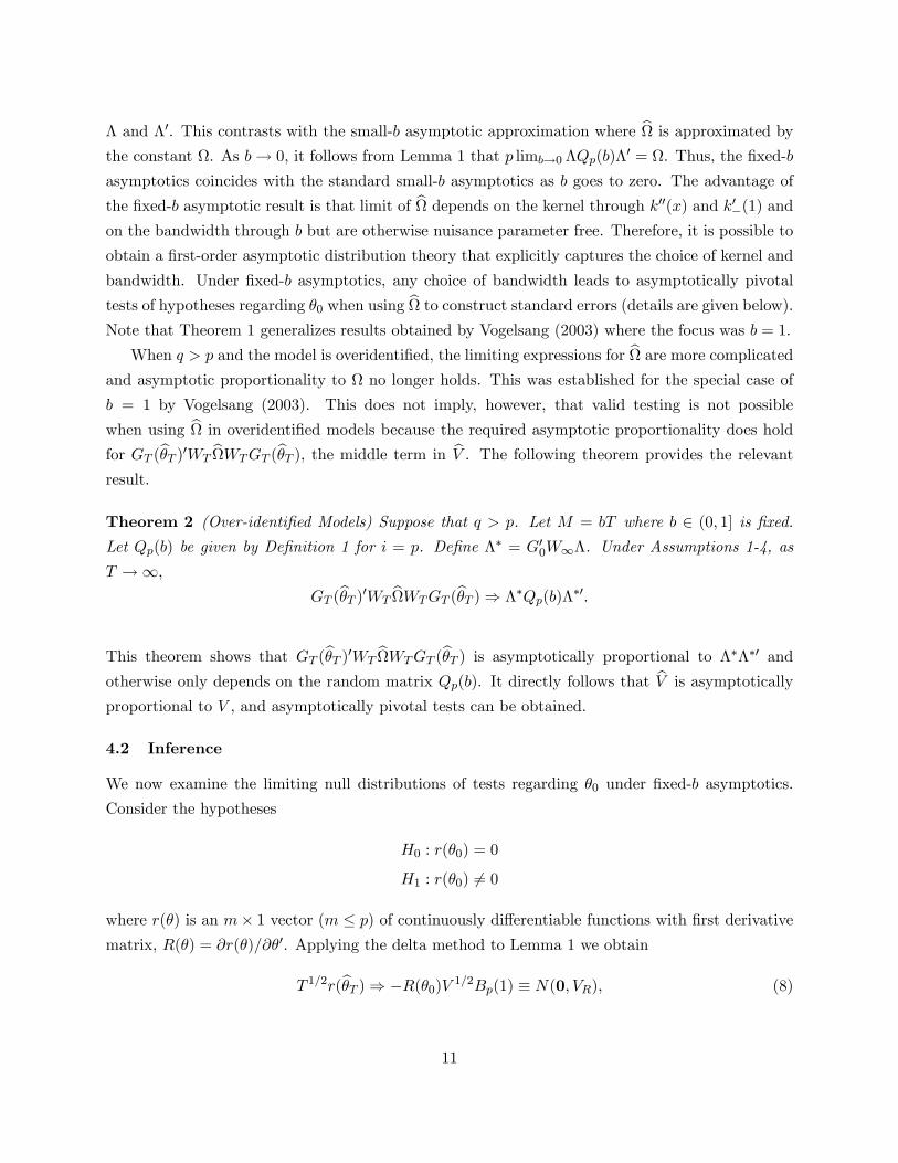
4.2 Inference

We now examine the limiting null distributions of tests regarding �0 under �xed-b asymptotics.

Consider the hypotheses

H0 : r(�0) = 0

H1 : r(�0) 6= 0

where r(�) is an m� 1 vector (m � p) of continuously di¤erentiable functions with �rst derivativematrix, R(�) = @r(�)=@�0. Applying the delta method to Lemma 1 we obtain

T 1=2r(b�T )) �R(�0)V 1=2Bp(1) � N(0; VR); (8)

11

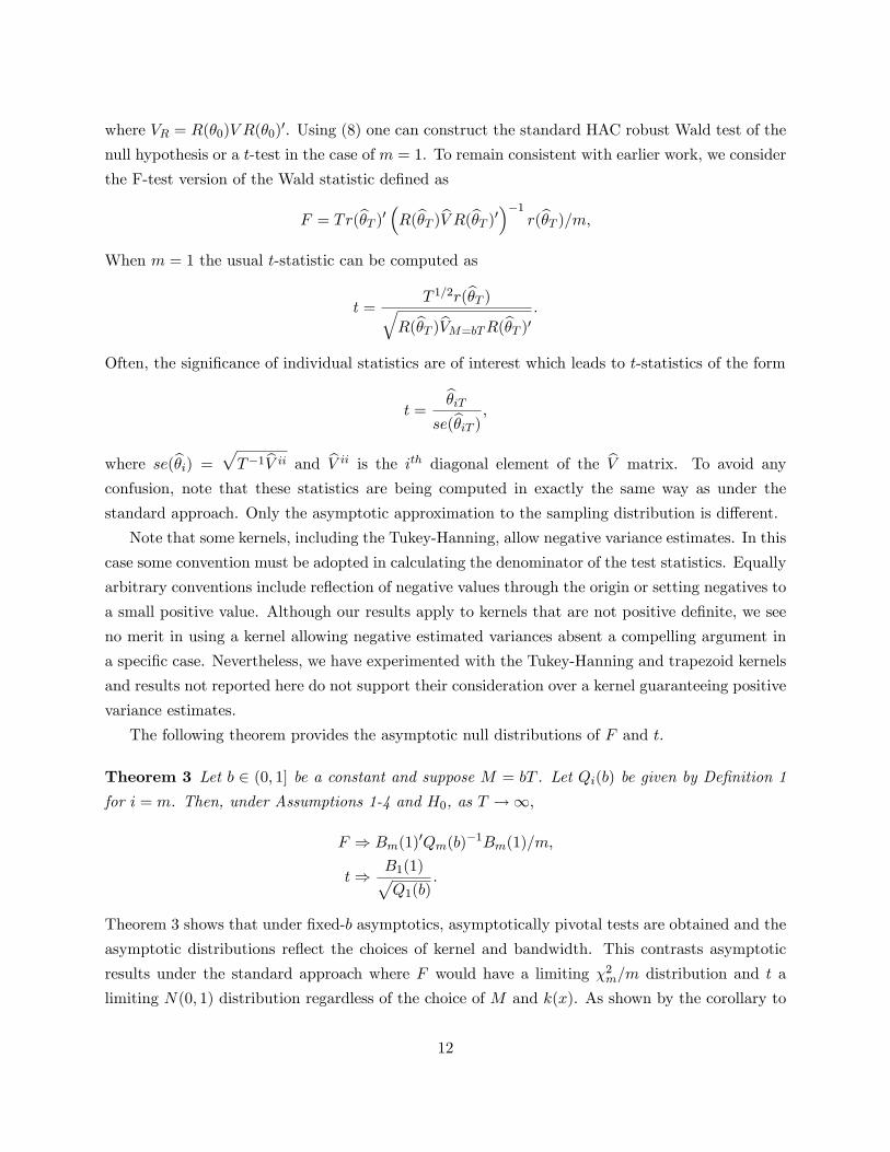
where VR = R(�0)V R(�0)0. Using (8) one can construct the standard HAC robust Wald test of the

null hypothesis or a t-test in the case of m = 1. To remain consistent with earlier work, we consider

the F-test version of the Wald statistic de�ned as

F = Tr(b�T )0 �R(b�T )bV R(b�T )0��1 r(b�T )=m;When m = 1 the usual t-statistic can be computed as

t =T 1=2r(b�T )q

R(b�T )bVM=bTR(b�T )0 :Often, the signi�cance of individual statistics are of interest which leads to t-statistics of the form

t =b�iT

se(b�iT ) ;where se(b�i) = p

T�1 bV ii and bV ii is the ith diagonal element of the bV matrix. To avoid any

confusion, note that these statistics are being computed in exactly the same way as under the

standard approach. Only the asymptotic approximation to the sampling distribution is di¤erent.

Note that some kernels, including the Tukey-Hanning, allow negative variance estimates. In this

case some convention must be adopted in calculating the denominator of the test statistics. Equally

arbitrary conventions include re�ection of negative values through the origin or setting negatives to

a small positive value. Although our results apply to kernels that are not positive de�nite, we see

no merit in using a kernel allowing negative estimated variances absent a compelling argument in

a speci�c case. Nevertheless, we have experimented with the Tukey-Hanning and trapezoid kernels

and results not reported here do not support their consideration over a kernel guaranteeing positive

variance estimates.

The following theorem provides the asymptotic null distributions of F and t.

Theorem 3 Let b 2 (0; 1] be a constant and suppose M = bT . Let Qi(b) be given by De�nition 1

for i = m. Then, under Assumptions 1-4 and H0, as T !1;

F ) Bm(1)0Qm(b)

�1Bm(1)=m;

t) B1(1)pQ1(b)

:

Theorem 3 shows that under �xed-b asymptotics, asymptotically pivotal tests are obtained and the

asymptotic distributions re�ect the choices of kernel and bandwidth. This contrasts asymptotic

results under the standard approach where F would have a limiting �2m=m distribution and t a

limiting N(0; 1) distribution regardless of the choice of M and k(x). As shown by the corollary to

12

Theorem 2, as b! 0, p limQm(b) = Im and the �xed-b asymptotics reduces to the standard small-

b asymptotics. Therefore, if a traditional bandwidth rule is used in conjunction with the �xed-b

asymptotics, in large samples the two asymptotic theories will coincide. However, because the value

of b is strictly greater than zero in practice, it is natural to expect �xed-b asymptotics to deliver

a more accurate approximation. The simulations results reported in Section 5 and in the working

paper, Kiefer and Vogelsang (2002c), indicate that this is true in some Gaussian models. Finite

sample results reported by Ravikumar, Ray and Savin (2004) indicate that the �xed-b asymptotic

approximation can substantially reduce size distortions in tests of joint hypotheses especially when

the number of hypotheses being tested is large.

A theoretical comparison of the accuracy of the �xed-b asymptotics with the small-b asymp-

totics is not currently available because existing methods in higher order asymptotic expansions,

such as Edgeworth expansions, do not directly apply to the �xed-b asymptotic nesting given the

nonstandard nature of the distribution theory. Obtaining such theoretical results appears di¢ cult

although for the Gaussian local model and the special case of the Bartlett kernel with b = 1,

Jansson (2004) has shown that the error in rejection probability of F is O(T�1 log(T )). Phillips

et al. (2004) conjecture that this result can be strengthened to O(T�1) and can be generalized to

include b < 1 and other kernels besides the Bartlett kernel.

4.3 Asymptotic Critical Values

The limiting distributions given by Theorem 3 are nonstandard. Analytical forms of the densities

are not available with the exception of t for the case of the Bartlett kernel with b = 1 (see Abadir and

Paruolo, 2002 and Kiefer and Vogelsang, 2002b). However, because the limiting distributions are

simple functions of standard Brownian motions, critical values are easily obtained using simulations.

In the working paper we provide critical values for the t statistic for a selection of popular kernels

(see the formula appendix for formulas for the kernels). Additional critical values for the F test

will be made available in a follow-up paper.

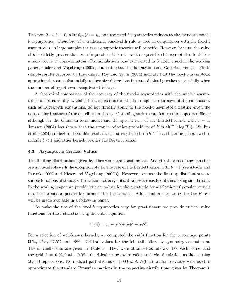
To make the use of the �xed-b asymptotics easy for practitioners we provide critical value

functions for the t statistic using the cubic equation

cv(b) = a0 + a1b+ a2b2 + a3b

3:

For a selection of well-known kernels, we computed the cv(b) function for the percentage points

90%, 95%, 97.5% and 99%. Critical values for the left tail follow by symmetry around zero.

The ai coe¢ cients are given in Table 1. They were obtained as follows. For each kernel and

the grid b = 0:02; 0:04; :::0:98; 1:0 critical values were calculated via simulation methods using

50,000 replications. Normalized partial sums of 1,000 i:i:d: N(0; 1) random deviates were used to

approximate the standard Brownian motions in the respective distributions given by Theorem 3.

13

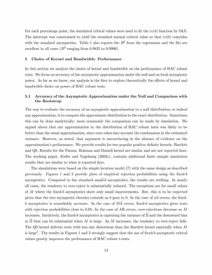
For each percentage point, the simulated critical values were used to �t the cv(b) function by OLS.

The intercept was constrained to yield the standard normal critical value so that cv(0) coincides

with the standard asymptotics. Table 1 also reports the R2 from the regressions and the �ts are

excellent in all cases (R2 ranging from 0.9825 to 0.9996).

5 Choice of Kernel and Bandwidth: Performance

In this section we analyze the choice of kernel and bandwidth on the performance of HAC robust

tests. We focus on accuracy of the asymptotic approximation under the null and on local asymptotic

power. As far as we know, our analysis is the �rst to explore theoretically the e¤ects of kernel and

bandwidth choice on power of HAC robust tests.

5.1 Accuracy of the Asymptotic Approximation under the Null and Comparison withthe Bootstrap

The way to evaluate the accuracy of an asymptotic approximation to a null distribution, or indeed

any approximation, is to compare the approximate distribution to the exact distribution. Sometimes

this can be done analytically; more commonly the comparison can be made by simulation. We

argued above that our approximation to the distribution of HAC robust tests was likely to be

better than the usual approximation, since ours takes into account the randomness in the estimated

variance. However, as noted, that argument is unconvincing in the absence of evidence on the

approximation�s performance. We provide results for two popular positive de�nite kernels: Bartlett

and QS. Results for the Parzen, Bohman and Daniell kernel are similar and are not reported here.

The working paper, Kiefer and Vogelsang (2002c), contains additional �nite sample simulation

results that are similar to what is reported here.

The simulations were based on the simple location model (7) with the same design as described

previously. Figures 1 and 2 provide plots of empirical rejection probabilities using the �xed-b

asymptotics. Compared to the standard small-b asymptotics, the results are striking. In nearly

all cases, the tendency to over-reject is substantially reduced. The exceptions are for small values

of M where the �xed-b asymptotics show only small improvements. But, this is to be expected

given that the two asymptotic theories coincide as b goes to 0. In the case of iid errors, the �xed-

b asymptotics is remarkably accurate. In the case of MA errors, �xed-b asymptotics gives tests

with rejection probabilities close to 0.05. In the case of AR errors, over-rejections decrease as M

increases. Intuitively, the �xed-b asymptotics is capturing the variance of b and the downward biasin b that can be substantial when M is large. As M increases, the tendency to over-reject falls.

The QS kernel delivers tests with less size distortions than the Bartlett kernel especially when M

is large7. The results in Figures 1 and 2 strongly suggest that the use of �xed-b asymptotic critical

values greatly improves the performance of HAC robust t-tests.

14

Note however, that as serial correlation in the errors becomes stronger, the tendency to over-

reject increases even when �xed-b critical values are used. The reason is that the functional central

limit theorem approximation begins to erode. Therefore, there may be potential for the bootstrap

to provide further re�nements in accuracy. The �xed-b asymptotics suggests that the bootstrap

could work because the HAC robust tests are asymptotically pivotal for any kernel and bandwidth.

Ideally, one would like to establish theoretically whether or not the bootstrap provides an asymptotic

re�nement. Such a theoretical exercise is well beyond the scope of this paper because higher order

expansions for �xed-b asymptotics have not been developed. Obtaining such expansions is an

important topic that deserves attention.

To show the potential of the bootstrap for HAC robust tests, we expanded our simulation study

to include the block bootstrap. We implemented the block bootstrap resampling scheme following

Götze and Künsch (1996) as follows. The original data, y1; y2; :::; yT is divided into T � l + 1overlapping blocks of length, l. For simplicity, we report results for l = 1; 4 both of which factor

into T = 50. T=l blocks are drawn randomly with replacement to form a bootstrap sample labeled

y�1; y�2; :::; y

�T . The bootstrap t statistic is computed as

t�Naive =

pT (b�� � y)pb� ;

where b�� = y� = T�1PTt=1 y

�t and b� is computed using formula (6) with f(y�t ; b��) = bu�t = y�t � b��.

We use the label "naive" because the bootstrap t-statistic is computed using the same formula forb as was used for the original data8.Empirical rejection probabilities using the naive bootstrap critical values are reported in Figures

1 and 2 and are labelled NBoot. There are some compelling patterns in the �gures. Contrary to

theoretical results by Davison and Hall (1993) and Götze and Künsch (1996) suggesting otherwise,

the naive bootstrap performs quite well; it dominates the standard normal approximation and has

rejection probabilities that are very similar to the �xed-b asymptotics. This is true even for the iid

(l = 1) bootstrap when the data is not iid. In addition, the fact that the naive bootstrap works

well when using the Bartlett kernel contrasts with conventional wisdom that claims bootstrapping

Bartlett kernel tests is not more accurate than the standard normal approximation.

It is quite striking how closely the naive bootstrap with l = 1 (the iid bootstrap) follows the

�xed-b approximation regardless of the error structure. Recent work by Goncalves and Vogelsang

(2004) has shown that this pattern is systematic. Goncalves and Vogelsang (2004) prove that the

naive bootstrap has the same �rst-order asymptotic distribution as the t-statistic under �xed-b

asymptotics including the case when l = 1. The simulations also suggest that the naive bootstrap

could be more accurate than �xed-b asymptotics with suitable choice of the block length. Focusing

on the cases of AR(1) errors with l = 4, notice that the naive bootstrap often has rejection

probabilities closer to 0.05 than �xed-b. While the naive bootstrap may provide a re�nement

15

over the �xed-b asymptotics, such a re�nement has not been formally established. Higher order

properties of the naive bootstrap under �xed-b asymptotics is a very interesting, but potentially

di¢ cult, area where more work is needed.

5.2 Local Asymptotic Power

Whereas the existing HAC literature has almost exclusively focused on the MSE of the HAC

estimator to guide the choice of kernel and bandwidth, a more relevant metric is to focus on the

power of the resulting tests. In this section we compare power of HAC robust t-tests using a

local asymptotic power analysis within the �xed-b asymptotic framework. Our analysis permits

comparison of power across bandwidths and across kernels. Such a comparison is not possible

using the traditional �rst-order small-b asymptotics because local asymptotic power is the same for

all bandwidths and kernels.

For clarity, we restrict attention to linear regression models. Given the results in Theorem 1,

the derivations in this section are very simple extensions of results given by Kiefer and Vogelsang

(2002b). Therefore, details are kept to a minimum. Consider the regression model

yt = x0t�0 + ut (9)

with �0 and xt p � 1 vectors. In terms of the general model we have f(vt; �0) = xt (yt � x0t�0).Without loss of generality, we focus on �i0, one element of �; and consider null and alternative

hypotheses

H0 : �i0 � 0

H1 : �i0 = cT�1=2

where c > 0 is a constant. If the regression model satis�es Assumptions 1 through 4, then we can

use the results of Theorem 1 and results from Kiefer and Vogelsang (2002b) to easily establish that

under the local alternative, H1, as T !1;

t) � +B1(1)pQ1(b)

; (10)

where � = c=pV ii.

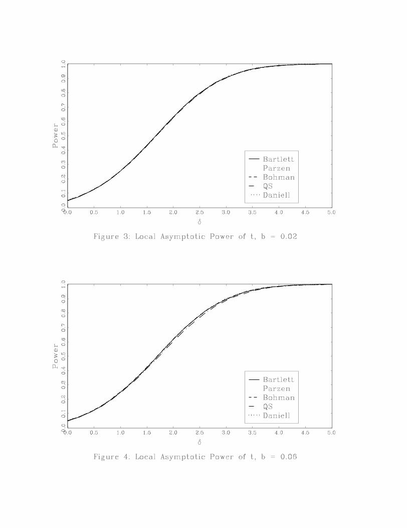
Asymptotic power curves can be computed for given bandwidths and kernels by simulating

the asymptotic distribution of t based on (10) for a range of values for � and computing rejection

probabilities with respect to the relevant null critical value. Using the same simulation methods as

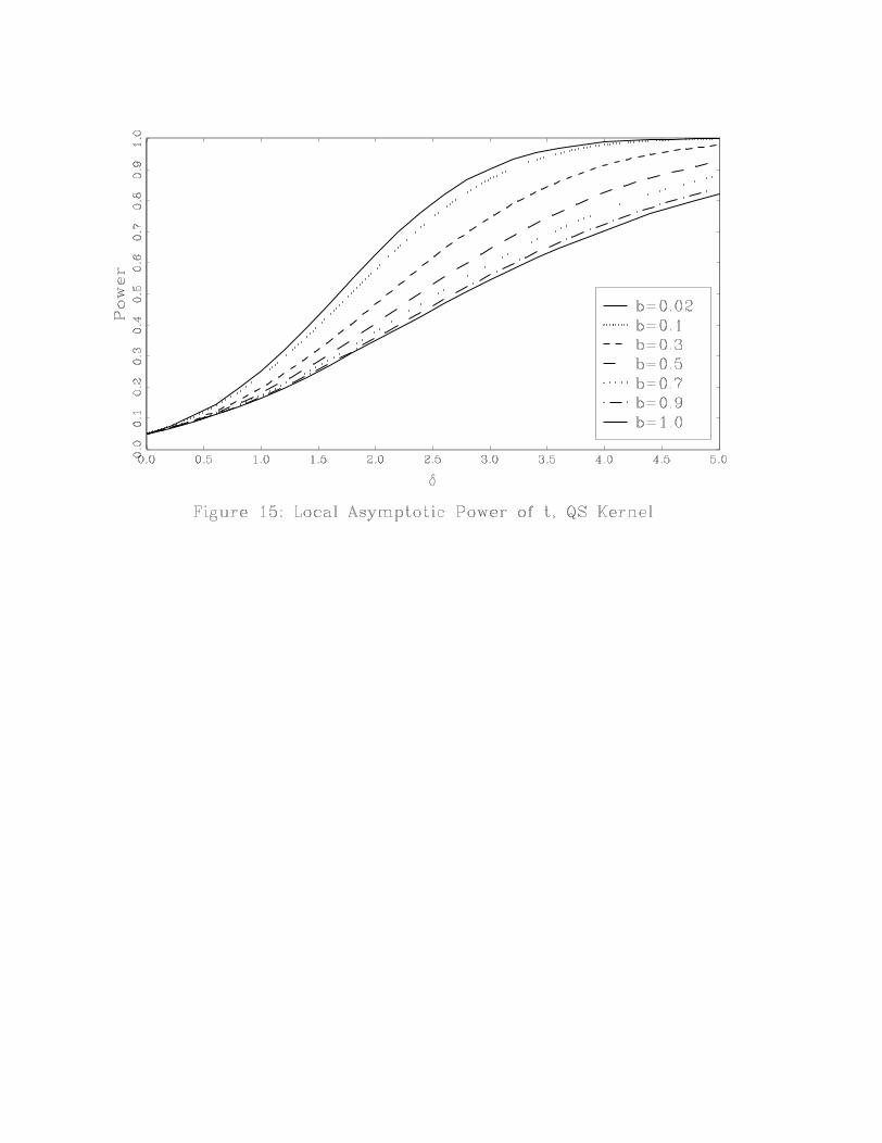
for the asymptotic critical values, local asymptotic power was computed for � = 0; 0:2; 0:4; :::; 4:8; 5:0

using 5% asymptotic null critical values.

16

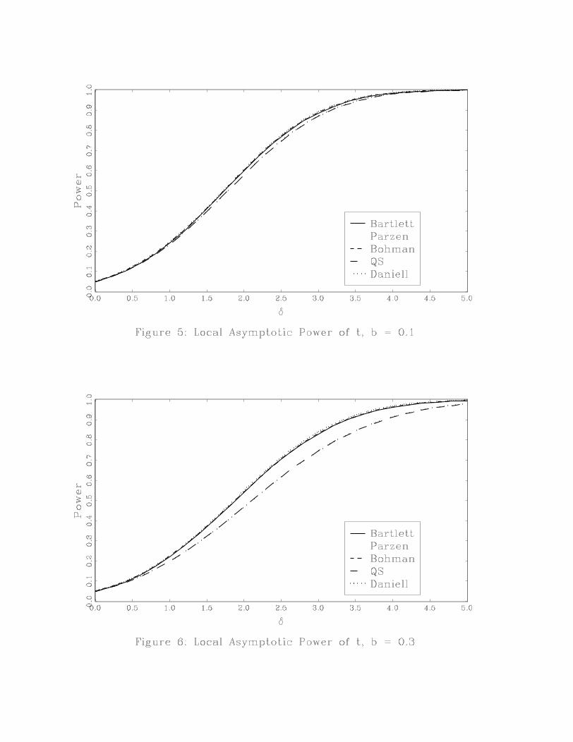
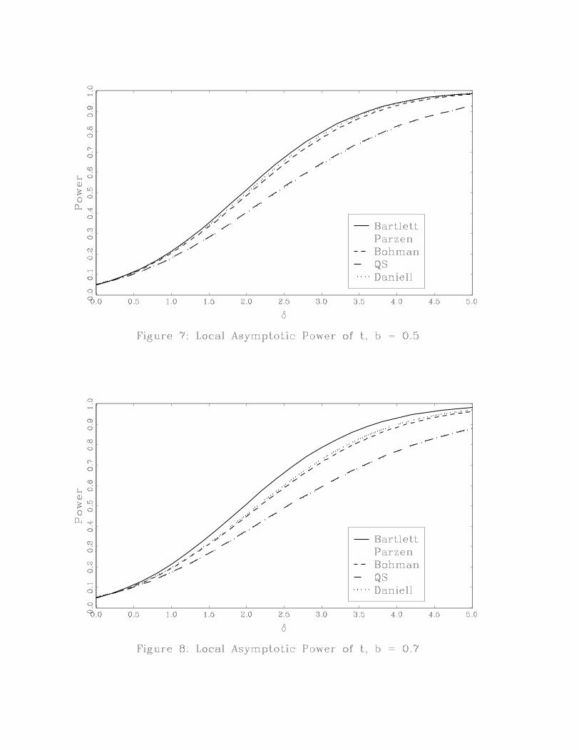
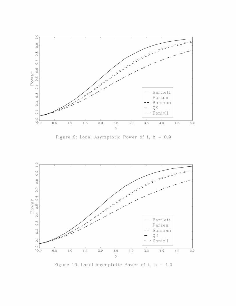
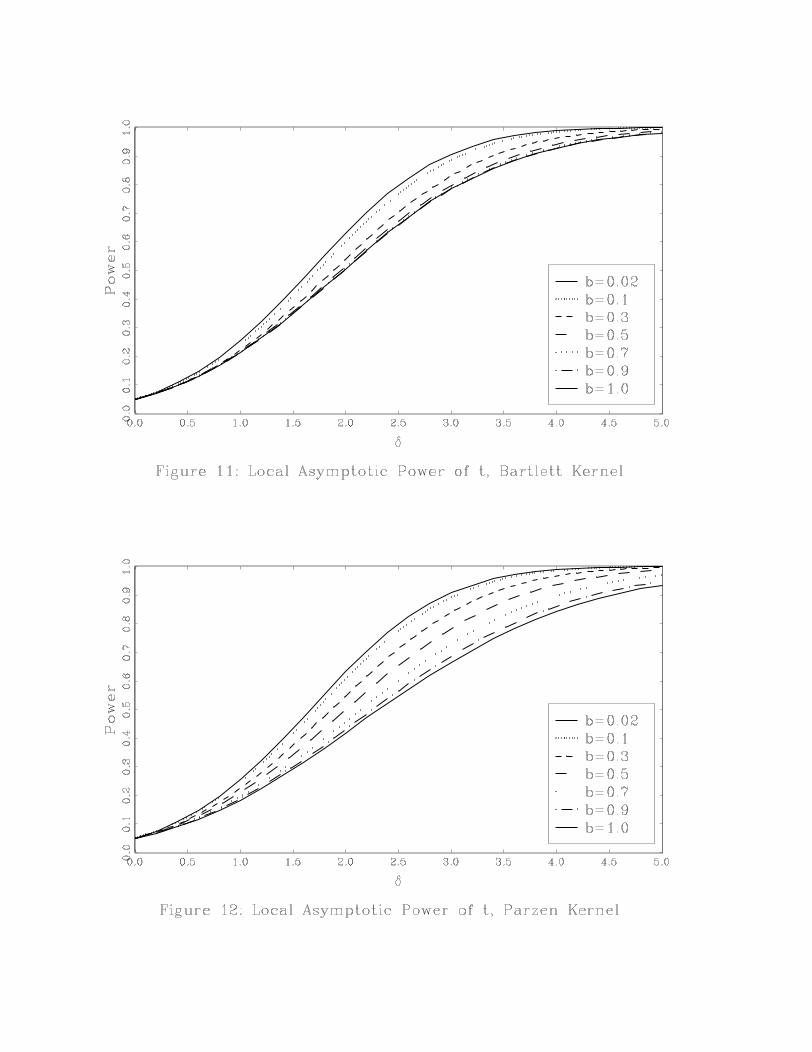
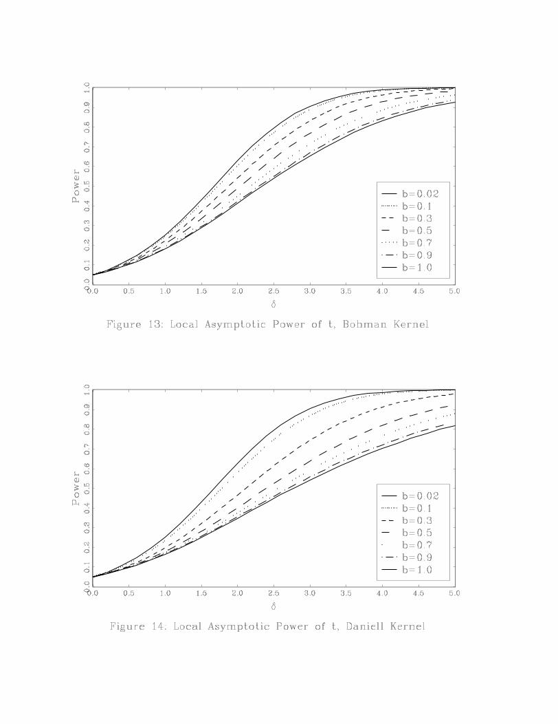
The power results are reported in two ways. Figures 3-10 plot power across the kernels for a

given value of b. Figures 11-15 plot power across values of b for a given kernel. Figures 3-10 show

that for small bandwidths, power is essentially the same across kernels. As b increases, it becomes

clear that the Bartlett kernel has the highest power while the QS and Daniell kernels have the

lowest power. If power is the criterion used to choose a test, then the Bartlett kernel is the best

choice within this set of �ve kernels. If we compare the Bartlett and QS kernels, we see that the

power ranking of these kernels is the reverse of their ranking based on accuracy of the asymptotic

approximation under the null.

Figures 11-15 show how the choice of bandwidth a¤ects power. Regardless of the kernel, power

is highest for small bandwidths and lowest for large bandwidths and power is decreasing in b: These

�gures also show that power of the Bartlett kernel is least sensitive to b whereas power of the

QS and Daniell kernels is the most sensitive to b. Again, power rankings of b are the opposite of

rankings of b based on accuracy of the asymptotic approximation under the null.

5.3 Size-Power Trade-o¤

The �nite sample simulations and local asymptotic power calculations clearly indicate a trade-o¤

between size distortions and power with regard to choice of kernel and bandwidth when using �xed-

b critical values. Smaller bandwidths lead to tests with higher power but at the cost of greater

size distortions whereas larger bandwidths lead to tests with less size distortions but lower power.

Similar trade-o¤s occur across kernels9. Balancing the size-power trade-o¤ in some systematic

way could lead to the development of useful bandwidth rules that deliver tests with desirable

properties10. Indeed, for the exponentiated Bartlett kernel, Phillips et al. (2004) propose a data

dependent rule for the choice of exponent that minimizes a loss function that is a weighted sum

of type I and type II errors. They develop higher-order expansions within the �xed-exponent

asymptotic framework and use these expansions to analytically quantify their loss function. The

authors conjecture that their results can be extended to traditional kernels via �xed-b asymptotics.

Thus it seems promising that �xed-b asymptotics can be used to develop data dependent bandwidth

rules that balance size distortion and power.

6 Conclusions

We have provided a new approach to the asymptotic theory of HAC robust testing. We consider

tests based on the popular nonparametric kernel estimates of the standard errors. We are not

proposing new tests but rather we propose a new asymptotic theory for these well-known tests.

Our results are general enough to apply to stationary models estimated by GMM. In our approach,

b, the ratio of bandwidth to sample size is held constant when deriving the asymptotic behavior

of the relevant covariance matrix estimator (i.e. zero frequency spectral density estimator). Thus

17

we label our asymptotic framework ��xed-b�asymptotics. In standard asymptotics, b is sent to

zero and can be viewed as a �small-b�asymptotic framework. Fixed-b asymptotics improves upon

two well-known problems with the standard approach. First, as has been well documented in

the literature, the standard asymptotic approximation of the sampling behavior of tests is often

poor. Second, the kernel and bandwidth choice do not appear in the approximate distribution,

leaving the standard theory silent on the choice of kernel and bandwidth with respect to properties

of the tests. Our theory leads to approximate distributions that explicitly depend on the kernel

and bandwidth. The new approximation performs much better and gives insight into the choice

of kernel and bandwidth with respect to test behavior. Once the higher-order results of Phillips

et al. (2004) have been extended to the �xed-b framework, data dependent bandwidth rules that

balance size distortion and power can be developed. In addition, �xed-b asymptotics should be

useful in explaining the performance of the naive bootstrap when applied to HAC robust tests.

The new approximations should be used for HAC robust test statistics for any choice of kernel

and bandwidth. The �xed-b approximation is an unambiguous improvement over the standard

normal approximation in most cases considered. We show that size distortions are reduced when

large bandwidths are used, but so is asymptotic power. Generally there is a trade-o¤ in bandwidth

and kernel choice between size (the accuracy of the approximation) and power. Among a group of

popular kernels, the QS kernel leads to the least size distortion, while the Bartlett kernel leads to

tests with highest power (and generally acceptable size distortion when large bandwidths are used).

7 Appendix: Proofs

We �rst de�ne some relevant functions and derive preliminary results before proving the lemma

and theorems. De�ne the functions

k� (x) = k�xb

�;

Kij = k

�i� jbT

�= k�

�i� jT

�;

�2Kij = (Kij �Ki;j+1)� (Ki+1;j �Ki+1;j+1) ;

D�T (r) = T2

��k��[rT ] + 1

T

�� k�

�[rT ]

T

����k��[rT ]

T

�� k�

�[rT ]� 1T

���:

Notice that

T 2�2Kij = �D�T�i� jT

�:

Because k(r) is an even function around r = 0,D�T (�r) = D�T (r). If k�00(r) exists then limT!1D�T (r) =k�00(r) by the de�nition of the second derivative. If k�00(r) is continuous, then D�T (r) converges to

k�00(r) uniformly in r. De�ne the stochastic process

XT (r) = GT (b�T )0WTT1=2g[rT ](�0)

18

for 1T � r � 1 and XT (r) = 0 for 0 � r < 1

T (i.e. set g0(�0) = 0). It directly follows from

Assumptions 2, 3 and 4 that

XT (r)) G00W1�Bq(r) � ��Bp(r): (11)

Proof of Lemma 1: Setting t = T , multiplying both sides of (4) by GT (b�T )0WT , and using the

�rst-order condition GT (b�T )0WT gT (b�T ) = 0 gives0 = GT (b�T )0WT gT (�0) +GT (b�T )0WTGT (b�T ; �0; �T )(b�T � �0): (12)

Solving (12) for (b�T � �0) and scaling by T 1=2 givesT 1=2(b�T � �0) = �[G0T (b�T )WTGT (b�T ; �0; �T )]�1G0T (b�T )WTT

1=2gT (�0)

= �[GT (b�T )0WTGT (b�T ; �0; �T )]�1XT (1): (13)

Because p limGT (b�T )0WTGT (b�T ; �0; �T ) = G00W1G0 by Assumptions 3 and 4, it follows from (11)

that

T 1=2(b�T � �0)) ��G00W1G0

��1��Bp(1):

We now prove Theorem 2. The proof of Theorem 1 follows using similar arguments and is

omitted.

Proof of Theorem 2: De�ne the random process eXT (r) = GT (b�T )0WTT1=2g[rT ](b�T ) for 1T � r � 1

and eXT (r) = 0 for 0 � r < 1T . Plugging in for g[rT ](

b�T ) using (4) giveseXT (r) = XT (r) +GT (b�T )0WTG[rT ](b�T ; �0; �T )T 1=2(b�T � �0)

= XT (r)�GT (b�T )0WTG[rT ](b�T ; �0; �T ) hGT (b�T )0WTGT (b�T ; �0; �T )i�1XT (1);using (13). It directly follows from Assumptions 3 and 4 and (11) that

eXT (r)) ��Bp(r)� rG00W1G0�G00W1G0

��1��Bp(1)

= �� (Bp(r)� rBp(1)) � �� eBp(r): (14)

Straightforward algebra gives

b = T�1Xj=�(T�1)

k

�j

bT

� b�j = T�1 TXi=1

TXj=1

f(vi; b�T )Kijf(vj ; b�T )0:

19

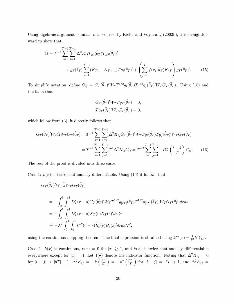
Using algebraic arguments similar to those used by Kiefer and Vogelsang (2002b), it is straightfor-

ward to show that

b = T�1 T�1Xi=1

T�1Xj=1

�2KijTgi(b�T )Tgj(b�T )0+ gT (b�T ) T�1X

i=1

(KTi �KT;i+1)Tgi(b�T )0 +0@ TXj=1

f(vj ; b�T )KjT1A gT (b�T )0: (15)

To simplify notation, de�ne Cij = GT (b�T )0WTT1=2gi(b�T )T 1=2gj(b�T )0WTGT (b�T ). Using (15) and

the facts that

GT (b�T )0WTTgT (b�T ) = 0;T gT (b�T )0WTGT (b�T ) = 0;

which follow from (3), it directly follows that

GT (b�T )0WTbWTGT (b�T ) = T�1 T�1X

i=1

T�1Xj=1

�2KijGT (b�T )0WTTgi(b�T )Tgj(b�T )0WTGT (b�T )= T�2

T�1Xi=1

T�1Xj=1

T 2�2KijCij = T�2

T�1Xi=1

T�1Xj=1

�D�T�i� jT

�Cij : (16)

The rest of the proof is divided into three cases.

Case 1: k(x) is twice continuously di¤erentiable. Using (16) it follows that

GT (b�T )0WTbWTGT (b�T )

= �Z 1

0

Z 1

0D�T (r � s)GT (b�T )0WTT

1=2g[rT ](b�T )T 1=2g[sT ](b�T )0WTGT (b�T )drds= �

Z 1

0

Z 1

0D�T (r � s) eXT (r) eXT (s)0drds

) ���Z 1

0

Z 1

0k�00(r � s) eBp(r) eBp(s)0drds��0;

using the continuous mapping theorem. The �nal expression is obtained using k�00(x) = 1b2k00(xb ).

Case 2: k(x) is continuous, k(x) = 0 for jxj � 1; and k(x) is twice continuously di¤erentiable

everywhere except for jxj = 1: Let 1(�) denote the indicator function. Noting that �2Kij = 0

for ji � jj > [bT ] + 1, �2Kij = �k�[bT ]bT

�= �k�

�[bT ]T

�for ji � jj = [bT ] + 1; and �2Kij =

20

hk�[bT ]bT

�� k

�[bT ]bT � 1

bT

�i+ k

�[bT ]bT

�=hk��[bT ]T

�� k�

�[bT ]T � 1

T

�i+ k�

�[bT ]T

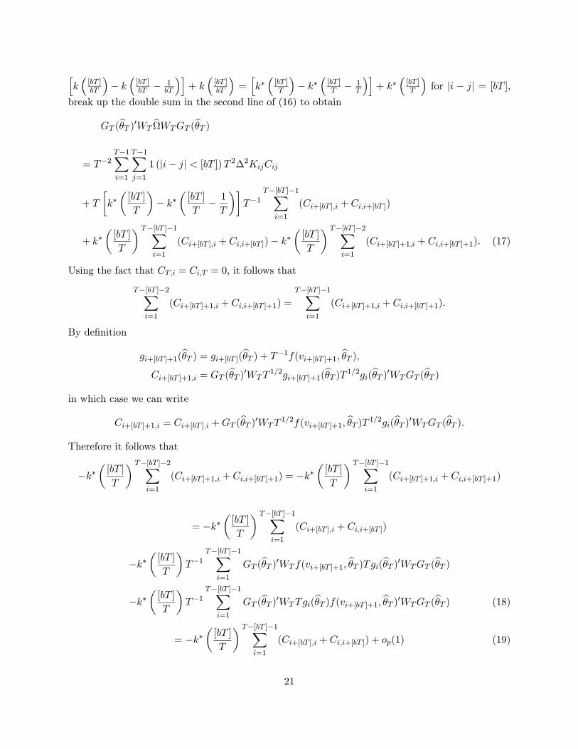
�for ji � jj = [bT ];

break up the double sum in the second line of (16) to obtain

GT (b�T )0WTbWTGT (b�T )

= T�2T�1Xi=1

T�1Xj=1

1 (ji� jj < [bT ])T 2�2KijCij

+ T

�k��[bT ]

T

�� k�

�[bT ]

T� 1

T

��T�1

T�[bT ]�1Xi=1

(Ci+[bT ];i + Ci;i+[bT ])

+ k��[bT ]

T

� T�[bT ]�1Xi=1

(Ci+[bT ];i + Ci;i+[bT ])� k��[bT ]

T

� T�[bT ]�2Xi=1

(Ci+[bT ]+1;i + Ci;i+[bT ]+1): (17)

Using the fact that CT;i = Ci;T = 0, it follows that

T�[bT ]�2Xi=1

(Ci+[bT ]+1;i + Ci;i+[bT ]+1) =

T�[bT ]�1Xi=1

(Ci+[bT ]+1;i + Ci;i+[bT ]+1):

By de�nition

gi+[bT ]+1(b�T ) = gi+[bT ](b�T ) + T�1f(vi+[bT ]+1; b�T );Ci+[bT ]+1;i = GT (b�T )0WTT

1=2gi+[bT ]+1(b�T )T 1=2gi(b�T )0WTGT (b�T )in which case we can write

Ci+[bT ]+1;i = Ci+[bT ];i +GT (b�T )0WTT1=2f(vi+[bT ]+1; b�T )T 1=2gi(b�T )0WTGT (b�T ):

Therefore it follows that

�k��[bT ]

T

� T�[bT ]�2Xi=1

(Ci+[bT ]+1;i + Ci;i+[bT ]+1) = �k��[bT ]

T

� T�[bT ]�1Xi=1

(Ci+[bT ]+1;i + Ci;i+[bT ]+1)

= �k��[bT ]

T

� T�[bT ]�1Xi=1

(Ci+[bT ];i + Ci;i+[bT ])

�k��[bT ]

T

�T�1

T�[bT ]�1Xi=1

GT (b�T )0WT f(vi+[bT ]+1; b�T )Tgi(b�T )0WTGT (b�T )�k�

�[bT ]

T

�T�1

T�[bT ]�1Xi=1

GT (b�T )0WTTgi(b�T )f(vi+[bT ]+1; b�T )0WTGT (b�T ) (18)

= �k��[bT ]

T

� T�[bT ]�1Xi=1

(Ci+[bT ];i + Ci;i+[bT ]) + op(1) (19)

21

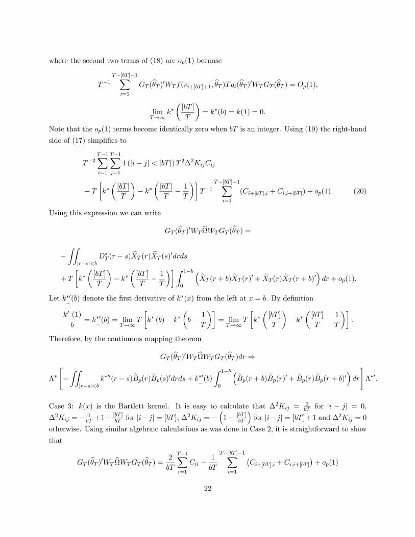
where the second two terms of (18) are op(1) because

T�1T�[bT ]�1X

i=1

GT (b�T )0WT f(vi+[bT ]+1; b�T )Tgi(b�T )0WTGT (b�T ) = Op(1);limT!1

k��[bT ]

T

�= k�(b) = k(1) = 0:

Note that the op(1) terms become identically zero when bT is an integer. Using (19) the right-hand

side of (17) simpli�es to

T�2T�1Xi=1

T�1Xj=1

1 (ji� jj < [bT ])T 2�2KijCij

+ T

�k��[bT ]

T

�� k�

�[bT ]

T� 1

T

��T�1

T�[bT ]�1Xi=1

(Ci+[bT ];i + Ci;i+[bT ]) + op(1): (20)

Using this expression we can write

GT (b�T )0WTbWTGT (b�T ) =

�ZZ

jr�sj<bD�T (r � s) eXT (r) eXT (s)0drds

+ T

�k��[bT ]

T

�� k�

�[bT ]

T� 1

T

��Z 1�b

0

� eXT (r + b) eXT (r)0 + eXT (r) eXT (r + b)0� dr + op(1):Let k�0_(b) denote the �rst derivative of k

�(x) from the left at x = b. By de�nition

k0�(1)

b= k�0_(b) = lim

T!1T

�k� (b)� k�

�b� 1

T

��= limT!1

T

�k��[bT ]

T

�� k�

�[bT ]

T� 1

T

��:

Therefore, by the continuous mapping theorem

GT (b�T )0WTbWTGT (b�T )dr )

��

"�ZZ

jr�sj<bk�00(r � s) eBp(r) eBp(s)0drds+ k�0_(b)Z 1�b

0

� eBp(r + b) eBp(r)0 + eBp(r) eBp(r + b)0� dr#��0:Case 3: k(x) is the Bartlett kernel. It is easy to calculate that �2Kij = 2

bT for ji � jj = 0,

�2Kij = � 1bT +1�

[bT ]bT for ji�jj = [bT ], �2Kij = �

�1� [bT ]

bT

�for ji�jj = [bT ]+1 and �2Kij = 0

otherwise. Using similar algebraic calculations as was done in Case 2, it is straightforward to show

that

GT (b�T )0WTbWTGT (b�T ) = 2

bT

T�1Xi=1

Cii �1

bT

T�[bT ]�1Xi=1

�Ci+[bT ];i + Ci;i+[bT ]

�+ op(1)

22

=2

b

Z 1

0

eXT (r) eXT (r)0dr � 1b

Z 1�b

0

� eXT (r + b) eXT (r)0 + eXT (r) eXT (r + b)0� dr + op(1)) ��

�2

b

Z 1

0

eBp(r) eBp(r)0dr � 1b

Z 1�b

0

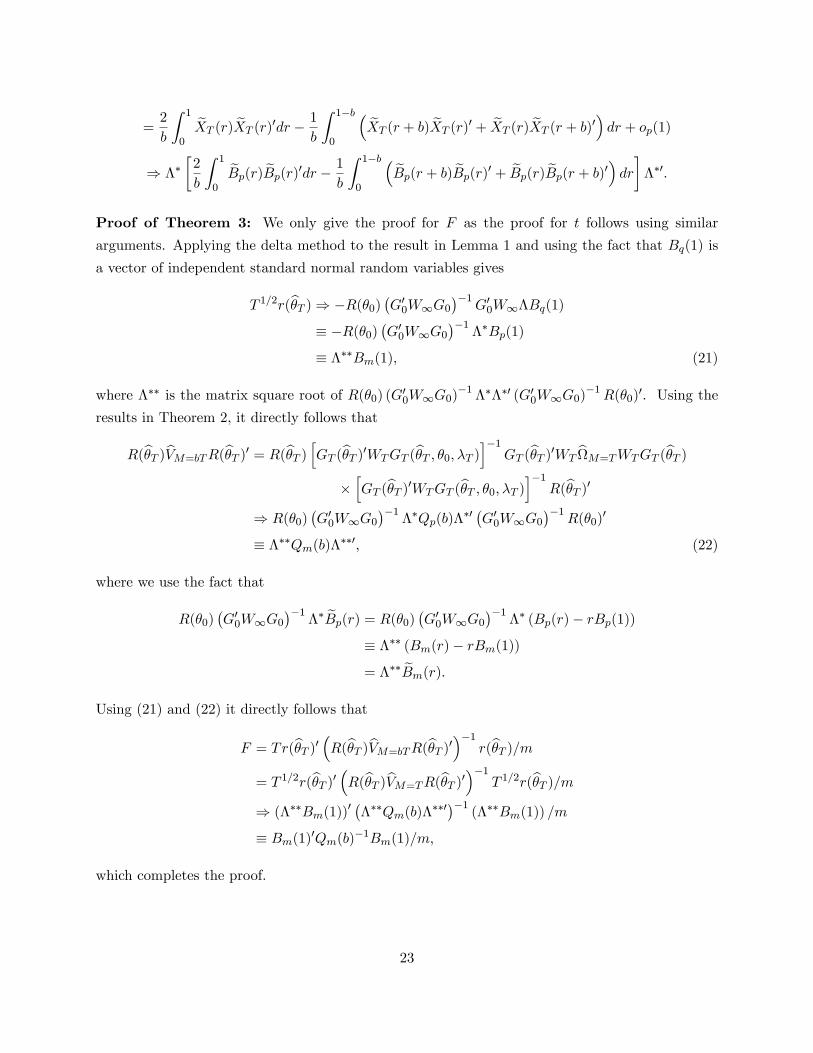
� eBp(r + b) eBp(r)0 + eBp(r) eBp(r + b)0� dr���0:Proof of Theorem 3: We only give the proof for F as the proof for t follows using similar

arguments. Applying the delta method to the result in Lemma 1 and using the fact that Bq(1) is

a vector of independent standard normal random variables gives

T 1=2r(b�T )) �R(�0)�G00W1G0

��1G00W1�Bq(1)

� �R(�0)�G00W1G0

��1��Bp(1)

� ���Bm(1); (21)

where ��� is the matrix square root of R(�0) (G00W1G0)�1 ����0 (G00W1G0)

�1R(�0)0: Using the

results in Theorem 2, it directly follows that

R(b�T )bVM=bTR(b�T )0 = R(b�T ) hGT (b�T )0WTGT (b�T ; �0; �T )i�1GT (b�T )0WTbM=TWTGT (b�T )

�hGT (b�T )0WTGT (b�T ; �0; �T )i�1R(b�T )0

) R(�0)�G00W1G0

��1��Qp(b)�

�0 �G00W1G0��1

R(�0)0

� ���Qm(b)���0; (22)

where we use the fact that

R(�0)�G00W1G0

��1�� eBp(r) = R(�0) �G00W1G0

��1�� (Bp(r)� rBp(1))

� ��� (Bm(r)� rBm(1))

= ��� eBm(r):Using (21) and (22) it directly follows that

F = Tr(b�T )0 �R(b�T )bVM=bTR(b�T )0��1 r(b�T )=m= T 1=2r(b�T )0 �R(b�T )bVM=TR(b�T )0��1 T 1=2r(b�T )=m) (���Bm(1))

0 ����Qm(b)���0��1 (���Bm(1)) =m� Bm(1)0Qm(b)�1Bm(1)=m;

which completes the proof.

23

Notes

1An alternative to the nonparametric approach has been advocated by den Haan and Levin(1997,1998). Following Berk (1974) and others in the time-series statistics literature, they proposeestimating the zero frequency spectral density parametrically using vector autoregression (VAR)models. They show that this parametric approach can achieve essentially the same generality asthe nonparametric approach if the VAR lag length increases with the sample size at a suitable rate.

2Additional discussion of this point is given by Cushing and McGarvey (1999, p. 80).

3An alternative approach to the �xed-b asymptotics is to consider higher order asymptotic ap-proximations in the small-b framework. For example, one could take the Edgeworth expansionsfrom the recent work by Velasco and Robinson (2001) and obtain a second order asymptotic ap-proximation for HAC robust tests that depends on the bandwidth and kernels. While this is apotentially fruitful approach, it is complicated by the need to estimate the second derivative of thespectral density.

4This common misperception is an unfortunate result of a folk-lore in the econometrics literaturethat states that �as M increases, bias in b decreases but variance increases.� This folk-lore isquite misleading although the source is easy to pinpoint. A careful reader of Priestley (1981) willrepeatedly see the phrase �asM increases, bias in b decreases but variance increases�. This phraseis completely correct if, as in Priestley (1981), one is discussing the properties of spectral densityestimators at non-zero frequencies or, in the case of known mean zero data, at the zero frequency.However, this phrase does not apply to zero frequency estimators computed using demeaned dataas is the case in GMM models. This fact is well known and has been nicely illustrated by Figure2 in Ng and Perron (1996) where plots of the exact bias and variance of b are given for AR(1)processes.

5The results in this section are a �xed-b asymptotic analysis of nonparametric zero-frequencyspectral density estimators. Fixed-b asymptotic results for spectral density estimators at non-zerofrequencies have been obtained by Hashimzade and Vogelsang (2003).

6The standard notation for the commutation matrix is usually Kii (see Magnus and Neudecker(1999, p.46). We are using alternative notation because Kij is used for a di¤erent matrix in ourproofs.

7A recent paper by Müller (2004) provides a novel way of theoretically quantifying the sizerobustness properties of HAC robust tests as a function of the kernel and b. The robustness measureproposed by Müller (2004) closely matches the patterns seen in the �nite sample simulations.

8We considered implementing the recentered and rescaled version of the bootstrap as proposedby Götze and Künsch (1996). Because Götze and Künsch (1996) recommend using the block length,l, equal to the HAC bandwidth, M , it is di¢ cult to implement this bootstrap for the full range ofM values given in Figures 1 and 2. The problem is that for large values of M , l is so large that theresampling is based on a very small number of blocks and it breaks down. We leave a comparisonof the naive bootstrap and the Götze and Künsch (1996) bootstrap to future research.

24

9Simulations reported by Phillips et al. (2003) and Phillips et al. (2005) found a similar trade-o¤between size distortion and power with respect to the exponent of exponentiated kernels.

10In the context of trend function inference analyzed using �xed-b asymptotics, Bunzel andVogelsang (2005) propose a data dependent bandwidth rule that maximizes integrated power.They focus only on power because the class of tests they consider are very robust in terms of sizedistortions. Their approach does not naturally apply to the models in this paper because their sizecorrection technique does not easily apply to models with stochastic regressors.

25

References

Abadir, K. M. and Paruolo, P. (2002), Simple Robust Testing of Regression Hypotheses: a Com-

ment, Econometrica 70, 2097�2099.

Andrews, D. W. K. (1991), Heteroskedasticity and Autocorrelation Consistent Covariance Matrix

Estimation, Econometrica 59, 817�854.

Andrews, D. W. K. and Monahan, J. C. (1992), An Improved Heteroskedasticity and Autocorrela-

tion Consistent Covariance Matrix Estimator, Econometrica 60, 953�966.

Berk, K. N. (1974), Consistent Autoregressive Spectral Estimates, The Annals of Statistics 2, 489�

502.

Bunzel, H. and Vogelsang, T. J. (2005), Powerful Trend Function Tests That are Robust to Strong

Serial Correlation with an Application to the Prebisch-Singer Hypothesis, Journal of Business

and Economic Statistics, forthcoming.

Bunzel, H., Kiefer, N. M. and Vogelsang, T. J. (2001), Simple Robust Testing of Hypotheses in

Non-linear Models, Journal of American Statistical Association 96, 1088�1098.

Cushing, M. J. and McGarvey, M. G. (1999), Covariance Matrix Estimation, in L. Matyas (ed.),

Generalized Method of Moments Estimation, Cambridge University Press, New York.

Davison, A. C. and Hall, P. (1993), On Studentizing and Blocking Methods for Implementing the

Bootstrap with Dependent Data, Australian Journal of Statistics 35, 215�224.

de Jong, R. M. and Davidson, J. (2000), Consistency of Kernel Estimators of Heteroskedastic and

Autocorrelated Covariance Matrices, Econometrica 68, 407�424.

den Haan, W. J. and Levin, A. (1997), A Practictioner�s Guide to Robust Covariance Matrix

Estimation, in G. Maddala and C. Rao (eds), Handbook of Statistics: Robust Inference, Volume

15, Elsevier, New York, pp. 291�341.

den Haan, W. J. and Levin, A. (1998), Vector Autoregressive Covariance Matrix Estimation, work-

ing paper, International Finance Division, FED Board of Governors.

Gallant, A. (1987), Nonlinear Statistical Models, Wiley, New York.

Gallant, A. and White, H. (1988), A Uni�ed Theory of Estimation and Inference for Nonlinear

Dynamic Models, Basil Blackwell, New York.

26

Goncalves, S. and Vogelsang, T. J. (2004), Block Bootstrap Puzzles in HAC Robust Testing: The

Sophistication of the Naive Bootstrap, Working Paper, Department of Economics, Cornell

University.

Götze, F. and Künsch, H. R. (1996), Second-Order Correctness of the Blockwise Bootstrap for

Stationary Observations, Annals of Statistics 24, 1914�1933.

Hall, P. and Horowitz, J. L. (1996), Bootstrap Critical Values for Tests Based on Generalized

Method of Moments Estimators, Econometrica 64, 891�916.

Hansen, B. E. (1992), Consistent Covariance Matrix Estimation for Dependent Heterogenous

Processes, Econometrica 60, 967�972.

Hansen, L. P. (1982), Large Sample Properties of Generalized Method of Moments Estimators,

Econometrica 50, 1029�1054.

Hashimzade, N. and Vogelsang, T. J. (2003), A New Asymptotic Approximation for the Sampling

Behavior of Spectral Density Estimators, Working Paper, Department of Economics, Cornell

University.

Hashimzade, N., Kiefer, N. M. and Vogelsang, T. J. (2003), Moments of HAC Robust Covariance

Matrix Estimators Under Fixed-b Asymptotics, Working Paper, Department of Economics,

Cornell University.

Heyde, C. (1997), Quasi-Likelihood and its Application. A General Approach to Optimal Parameter

Estimation, Springer, New York.

Inoue, A. and Shintani, M. (2004), Bootstrapping GMM Estimators for Time Series, Journal of

Econometrics. forthcoming.

Jansson, M. (2002), Consistent Covariance Estimation for Linear Processes, Econometric Theory

18, 1449�1459.

Jansson, M. (2004), The Error Rejection Probability of Simple Autocorrelation Robust Tests,

Econometrica 72, 937�946.

Kiefer, N. M. and Vogelsang, T. J. (2002)a, Heteroskedasticity-Autocorrelation Robust Standard

Errors Using the Bartlett Kernel Without Truncation, Econometrica 70, 2093�2095.

Kiefer, N. M. and Vogelsang, T. J. (2002)b, Heteroskedasticity-Autocorrelation Robust Testing

Using Bandwidth Equal to Sample Size, Econometric Theory 18, 1350�1366.

27

Kiefer, N. M. and Vogelsang, T. J. (2005), A New Asymptotic Theory for Heteroskedasiticy-

Autocorrelation Robust Tests, Econometric Theory, forthcoming.

Kiefer, N. M., Vogelsang, T. J. and Bunzel, H. (2000), Simple Robust Testing of Regression Hy-

potheses, Econometrica 68, 695�714.

Magnus, J. R. and Neudecker, H. (1999),Matrix Di¤erential Calculus with Applications in Statistics

and Econometrics, Wiley, New York.

Müller, U. K. (2004), A Theory of Robust Long-Run Variance Estimation, mimeo, Department of

Economics, Princeton University.

Neave, H. R. (1970), An Improved Formula for the Asymptotic Variance of Spectrum Estimates,

Annals of Mathematical Statistics 41, 70�77.

Newey, W. K. and McFadden, D. L. (1994), Large Sample Estimation and Hypothesis Testing,

in R. Engle and D. L. McFadden (eds), Handbook of Econometrics, Vol. 4, Elsevier Science

Publishers, Amseterdam, The Netherlands, pp. 2113�2247.

Newey, W. K. and West, K. D. (1987), A Simple, Positive Semi-De�nite, Heteroskedasticity and

Autocorrelation Consistent Covariance Matrix, Econometrica 55, 703�708.

Newey, W. K. and West, K. D. (1994), Automatic Lag Selection in Covariance Estimation, Review

of Economic Studies 61, 631�654.

Ng, S. and Perron, P. (1996), The Exact Error in Estimating the Spectral Density at the Origin,

Journal of Time Series Analysis 17, 379�408.

Phillips, P. C. B. and Durlauf, S. N. (1986), Multiple Regression with Integrated Processes, Review

of Economic Studies 53, 473�496.

Phillips, P. C. B., Sun, Y. and Jin, S. (2003), Consistent HAC Estimation and Robust Regres-

sion Testing Using Sharp Origin Kernels with No Truncation, Working Paper, Department of

Economics, Yale University.

Phillips, P. C. B., Sun, Y. and Jin, S. (2004), Improved HAR Inference Using Power Kernels without

Truncation, Working Paper, Department of Economics, Yale University.

Phillips, P. C. B., Sun, Y. and Jin, S. (2005), Spectral Density Estimation and Robust Hypoth-

esis Testing using Steep Origin Kernels without Truncation, International Economic Review,

forthcoming.

Priestley, M. B. (1981), Spectral Analysis and Time Series, Vol. 1, Academic Press, New York.

28

Ravikumar, B., Ray, S. and Savin, N. E. (2004), Robust Wald Tests and the Curse of Dimensionality,

Working paper, Department of Economics, University of Iowa.

Robinson, P. (1998), Inference-Without Smoothing in the Presence of Nonparametric Autocorrela-

tion, Econometrica 66, 1163�1182.

Simono¤, J. (1993), The Relative Importance of Bias and Variability in the Estimation of the

Variance of a Statistic, The Statistician 42, 3�7.

Velasco, C. and Robinson, P. M. (2001), Edgeworth Expansions for Spectral Density Estimates and

Studentized Sample Mean, Econometric Theory 17, 497�539.

Vogelsang, T. J. (2003), Testing in GMM Models Without Truncation, Advances in Econometrics,

Maximum Likelihood Estimation of Misspeci�ed Models: Twenty Years Later, Vol. 17, pp. 199�

233.

White, H. (1984), Asymptotic Theory for Econometricians, Academic Press, New York.

29

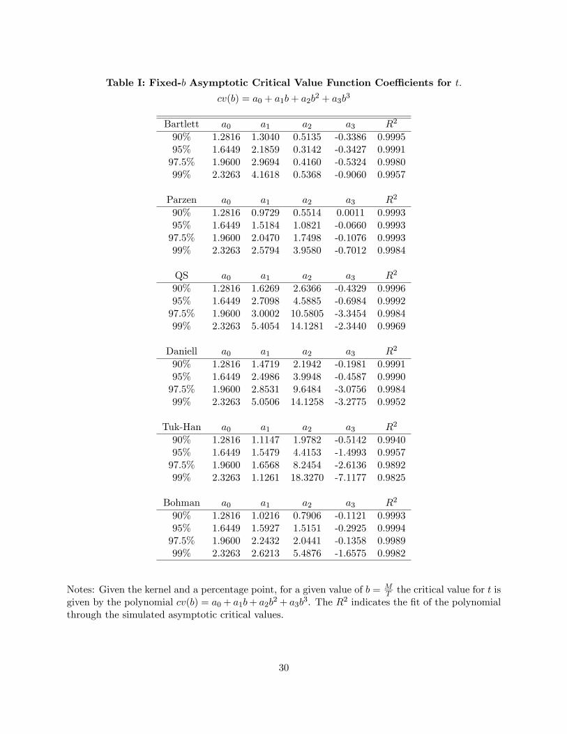
Table I: Fixed-b Asymptotic Critical Value Function Coe¢ cients for t.

cv(b) = a0 + a1b+ a2b2 + a3b

3

Bartlett a0 a1 a2 a3 R2

90% 1.2816 1.3040 0.5135 -0.3386 0.999595% 1.6449 2.1859 0.3142 -0.3427 0.999197.5% 1.9600 2.9694 0.4160 -0.5324 0.998099% 2.3263 4.1618 0.5368 -0.9060 0.9957

Parzen a0 a1 a2 a3 R2

90% 1.2816 0.9729 0.5514 0.0011 0.999395% 1.6449 1.5184 1.0821 -0.0660 0.999397.5% 1.9600 2.0470 1.7498 -0.1076 0.999399% 2.3263 2.5794 3.9580 -0.7012 0.9984

QS a0 a1 a2 a3 R2

90% 1.2816 1.6269 2.6366 -0.4329 0.999695% 1.6449 2.7098 4.5885 -0.6984 0.999297.5% 1.9600 3.0002 10.5805 -3.3454 0.998499% 2.3263 5.4054 14.1281 -2.3440 0.9969

Daniell a0 a1 a2 a3 R2

90% 1.2816 1.4719 2.1942 -0.1981 0.999195% 1.6449 2.4986 3.9948 -0.4587 0.999097.5% 1.9600 2.8531 9.6484 -3.0756 0.998499% 2.3263 5.0506 14.1258 -3.2775 0.9952

Tuk-Han a0 a1 a2 a3 R2

90% 1.2816 1.1147 1.9782 -0.5142 0.994095% 1.6449 1.5479 4.4153 -1.4993 0.995797.5% 1.9600 1.6568 8.2454 -2.6136 0.989299% 2.3263 1.1261 18.3270 -7.1177 0.9825

Bohman a0 a1 a2 a3 R2

90% 1.2816 1.0216 0.7906 -0.1121 0.999395% 1.6449 1.5927 1.5151 -0.2925 0.999497.5% 1.9600 2.2432 2.0441 -0.1358 0.998999% 2.3263 2.6213 5.4876 -1.6575 0.9982

Notes: Given the kernel and a percentage point, for a given value of b = MT the critical value for t is

given by the polynomial cv(b) = a0 + a1b+ a2b2 + a3b3. The R2 indicates the �t of the polynomialthrough the simulated asymptotic critical values.

30