A Tabu Search algorithm for the optimisation of telecommunication networks

蔣雅慈

Introduction

A single exchange (or single hub) network may lead to inefficiencies. [Luby & Dziatkjewicz, 1989], [Moondra, 1989]

The exchange can be duplicated.

Introduction (con.)

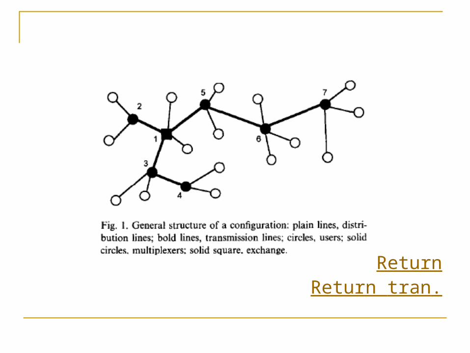
A suitable model of the overall structure will be provided by connecting a single exchange and a number of multiplexing centers and connecting to it all the users.

The major planning problem is to connect all the users to the exchange through a tree multiplexer network having an optimised overall cost.

ReturnReturn tran.

Introduction (con.)

Many combinatorial optimisation problems fall into the class of the NP-complete problems. [Garey & Johnson 1979]

Optimisation techniques based on linear programming. (Linear does not accurately represent the effective cost of the actual network).

Heuristic algorithms yield satisfactory results.

Introduction (con.) “add and drop” techniques. [Boorstin & Frank, 1977],

[Gerla & Kleinrock, 1977], [McGregor & Shen, 1977], [Costamagna, 1997], in this paper we refer to it as HAD.

HAD algorithm was compared with branch and bound technique. [Costamagna et al., 1990]

Recently, natural algorithms (GA [Celli et al., 1995], SA [Costamagna et al., 1995]) have been implemented.

In this paper a TS algorithm is discussed.

Problem definition and formulation

The function to be minimised represents the overall cost of the network, the sum of four components:

1. the cost of the distribution network. 2. the cost of the multiplexing centers. 3. the cost of the transport network. 4. the cost of multiplexer/demultiplexer equipment

located in the exchange.

graph

The cost of the distribution network

The sum of the costs of the links which connect all the users to the closest multiplexing center, and of the costs of the users’ terminals.

notation

N number of users

NN number of feasible locations of multiplexing centers

CF10 cost of the fiber-optic cable

D N*N matrix, dij, shortest path between ith and jth nodes

Y N*NN incidence matrix of the distribution network, yij = 1 if the ith user is connected to the jth multiplexing center

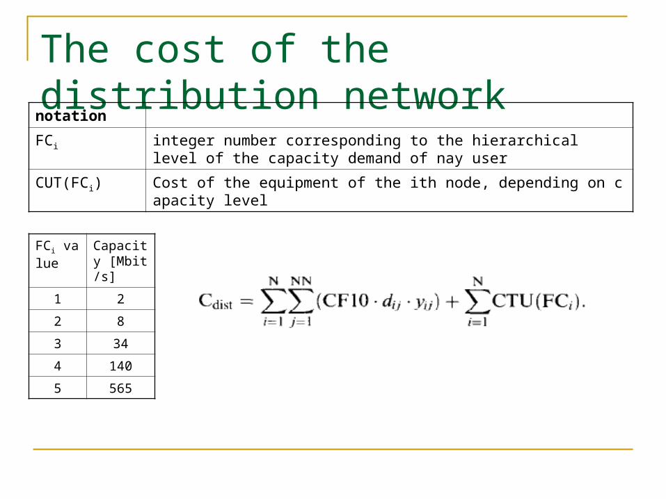
The cost of the distribution network

notation

FCi integer number corresponding to the hierarchical level of the capacity demand of nay user

CUT(FCi) Cost of the equipment of the ith node, depending on capacity level

FCi value

Capacity [Mbit/s]

1 2

2 8

3 34

4 140

5 565

The cost of multiplexing centers

notation

k capacity hierarchy index

CM(k) cost of the multiplexer with input capacity at hierarchy level k

S(k) integer variable used to compute the number of multiplexers needed, at input hierarchy level k: S(k) = 16 if k = 1 and S(k) = 4 if k = 2, 3, 4

Nkj Number of connections at input hierarchy level k connected to the jth multiplexing center

xj Activation index, showing if the jth multiplexing center has been activated (xj = 1 ) not ( xj = 0 )

The cost of multiplexing centers (con.)

The overall cost of the jth multiplexing center CMPj :

The cost of the transport network

The sum of the costs of the cables connecting the multiplexing centers to the exchange.

notation

CF50 cost of the fiber optic cable used to build the transport network

Z NN*NN incidence matrix representing the transport network: z ij = 1 if he ith multiplexing center is connected to the jth one

CTL(k) cost of the line terminal of hierarchy k

FTj capacity hierarchy level of output flow of the jth multiplexing center

The cost of demultiplexers

notation

CDMPXk Cost of multiplexing /demultiplexing equipment with hierarchy level equal to k in the exchange

Nkj Number of fibers at hierarchy level k connecting the jth multiplexing center and the exchange

Problem and constraints

Tabu Search A configuration of the network is a binary string,

whose size equals the number of feasible locations of multiplexing centers.

In TS methods (the problem is the binary string), a simple move: the change of one bit at a time.

This allows speeding up the execution of each iteration of the TS algorithm.

The variation of the network

The initial solution is a star configuration: all the users are directly connected to the exchange with a minimum spanning tree.

The binary string has zeroes everywhere, except in the bit corresponding to the location of the exchange, which equals 1.

At each step, add or drop one multiplexing center to the previous configuration.

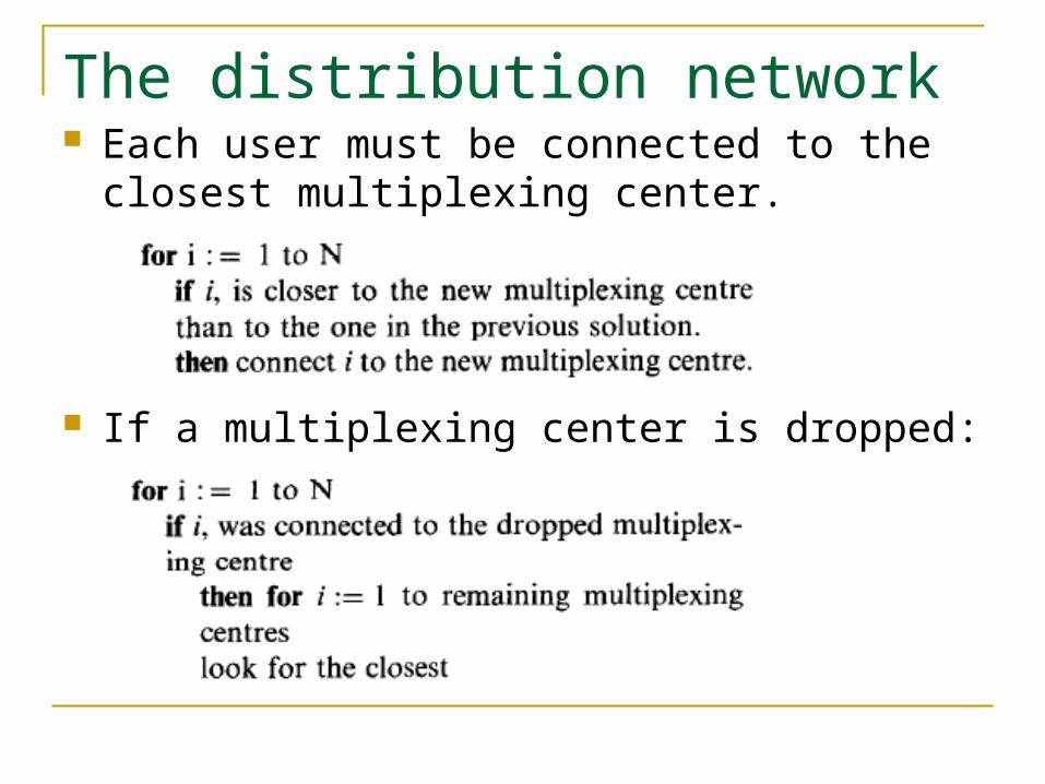
The distribution network Each user must be connected to the closest

multiplexing center.

If a multiplexing center is dropped:

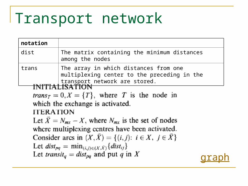
Transport network

notation

dist The matrix containing the minimum distances among the nodes

trans The array in which distances from one multiplexing center to the preceding in the transport network are stored.

graph

Multiplation/demultiplation

The equipment in each center is different from that used in the previous solution and must be re-designed.

For each activated center, the record of the cost, the number and type of the equipment, the input flows and the number of fiber-optic cables in output are needed.

Cost variation

The variation of the cost of the distribution network The variation of the cost of the transport network The variation of multiplexing and demultiplexing cost The saving in computational time increases according

to the growth in size of the network.

TS algorithm

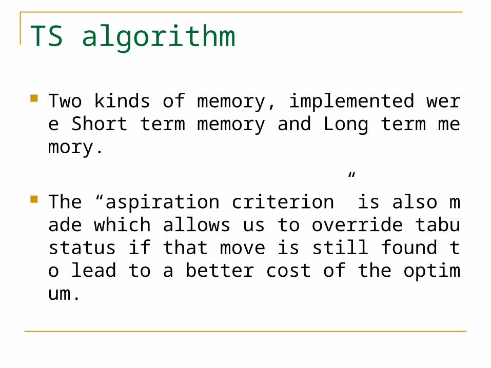
Two kinds of memory, implemented were Short term memory and Long term memory.

The “aspiration criterion” is also made which allows us to override tabu status if that move is still found to lead to a better cost of the optimum.

The choice of parameters

An extensive testing involving some networks of different sizes.

The implementation of the described algorithm has been proven to be very fast. [Celli & Costamagna, 1995], [Costamagna, 1997], [Costamagna et al., 1995]

The algorithm run 10000 iterations for each trial.

Short term memory

Smaller values of tabu_tenure cannot prevent cycling.

Larger values could forbid useful moves. Using a dynamically varying tabu_tenure has b

een tried. [Glover et al., 1993]

Long term memory

Transition frequencies and residence frequencies has been implemented. [Glover, 1994]

Many tests showed a better performance of the algorithm when absolute value of the transition frequencies has been used.

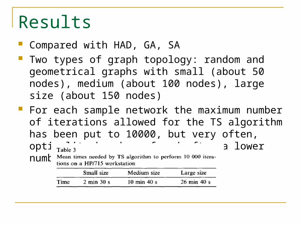
Results Compared with HAD, GA, SA Two types of graph topology: random and geometrical graphs

with small (about 50 nodes), medium (about 100 nodes), large size (about 150 nodes)

For each sample network the maximum number of iterations allowed for the TS algorithm has been put to 10000, but very often, optimality has been found after a lower number of iterations.

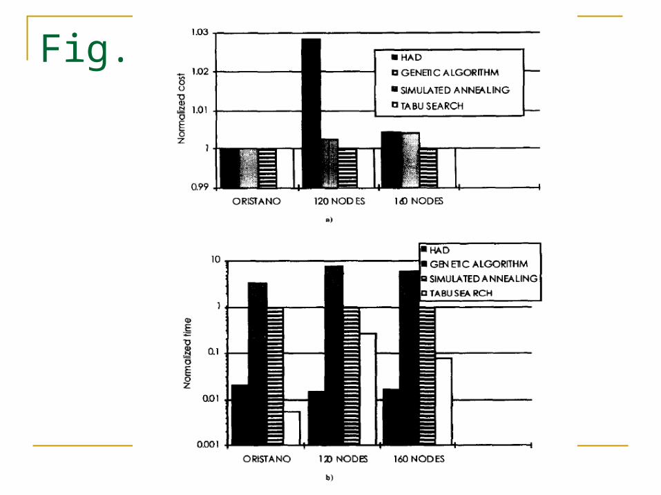
Fig. 2

Considerations on sample networks If the TS algorithm was forced to use only the

computational time needed by HAD, the configuration found by TS was better than the HAD one.

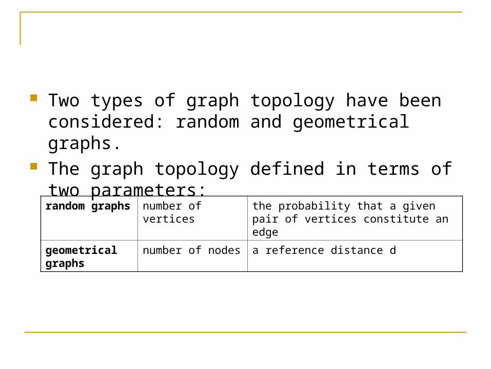
Two types of graph topology have been considered: random and geometrical graphs.

The graph topology defined in terms of two parameters:

random graphs number of vertices the probability that a given pair of vertices constitute an edge

geometrical graphs

number of nodes a reference distance d

Fig. 3(random) Fig. 4(geometrical)

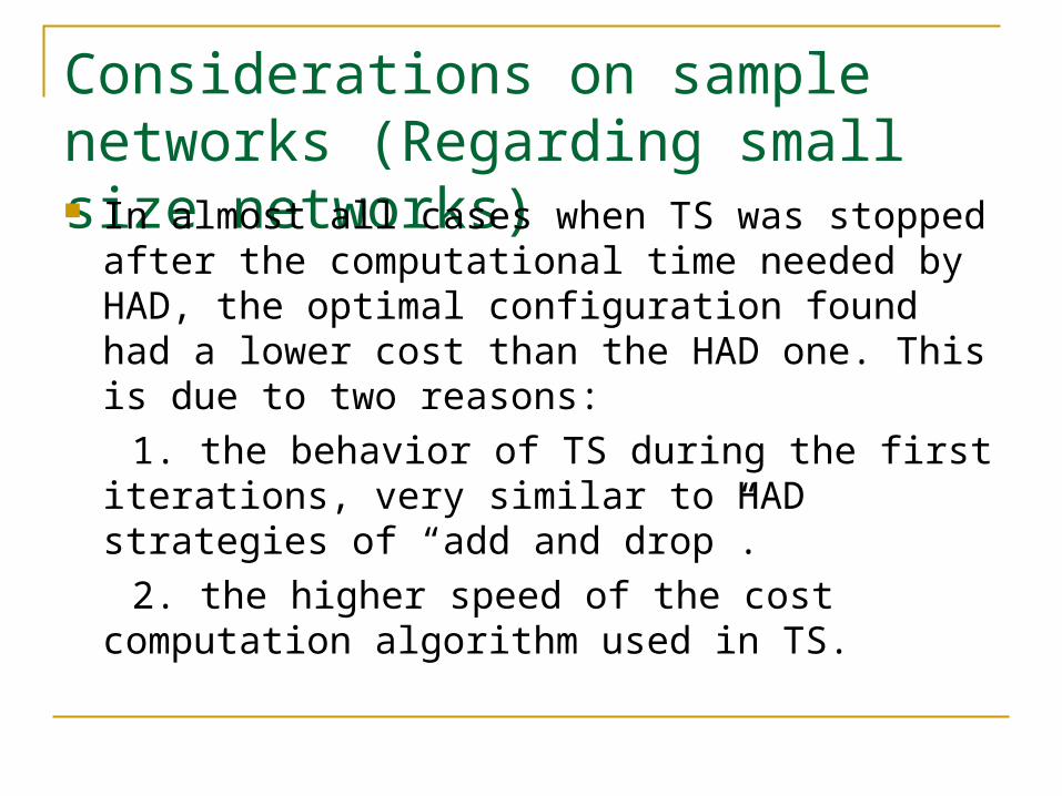
Considerations on sample networks (Regarding small size networks) In almost all cases when TS was stopped after the

computational time needed by HAD, the optimal configuration found had a lower cost than the HAD one. This is due to two reasons:

1. the behavior of TS during the first iterations, very similar to HAD strategies of “add and drop”.

2. the higher speed of the cost computation algorithm used in TS.

Considerations on sample networks (Regarding medium and large size random graphs) Medium size:

For a net work with 96 nodes the configuration found by TS has a cost 0.51% lower than SA’s, and 0.06% lower for a 100 node network.

Large size:

1. The random graphs TS performed better.

2. Very often TS was able to find better configurations than HAD and SA when stopped after their computational time.

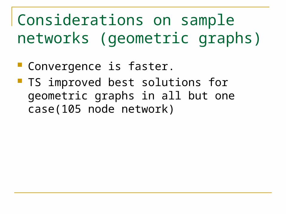
Considerations on sample networks (geometric graphs)

Convergence is faster. TS improved best solutions for geometric graphs in

all but one case(105 node network)

Conclusion

Computation times required by the TS method developed are on the average somewhat less than those required by the SA.

GA and SA methods required a large number of trials on a single problem with the same parameters setting.