approximating the minimum degree spanning tree to within one from the optimal degree r96922115...
TRANSCRIPT
Approximating the Minimum Degree Spanning Tree to within One from the Optimal Degree
R96922115 陳建霖R96922055 宋彥朋B93902023 楊鈞羽R96922074 郭慶徵R96922142 林佳慶

Authors
• Martin Furer Department of Computer Science and Engineering
The Pennsylvania State University
• Balaji Raghavachari Computer Science Department, EC 3.1
University of Texas at Dallas

Application
• Distribution of mail and news on the Internet
• Designing power grids

Similar approximation properties
• Edge coloring problem
• 3-colorability of planer graphs
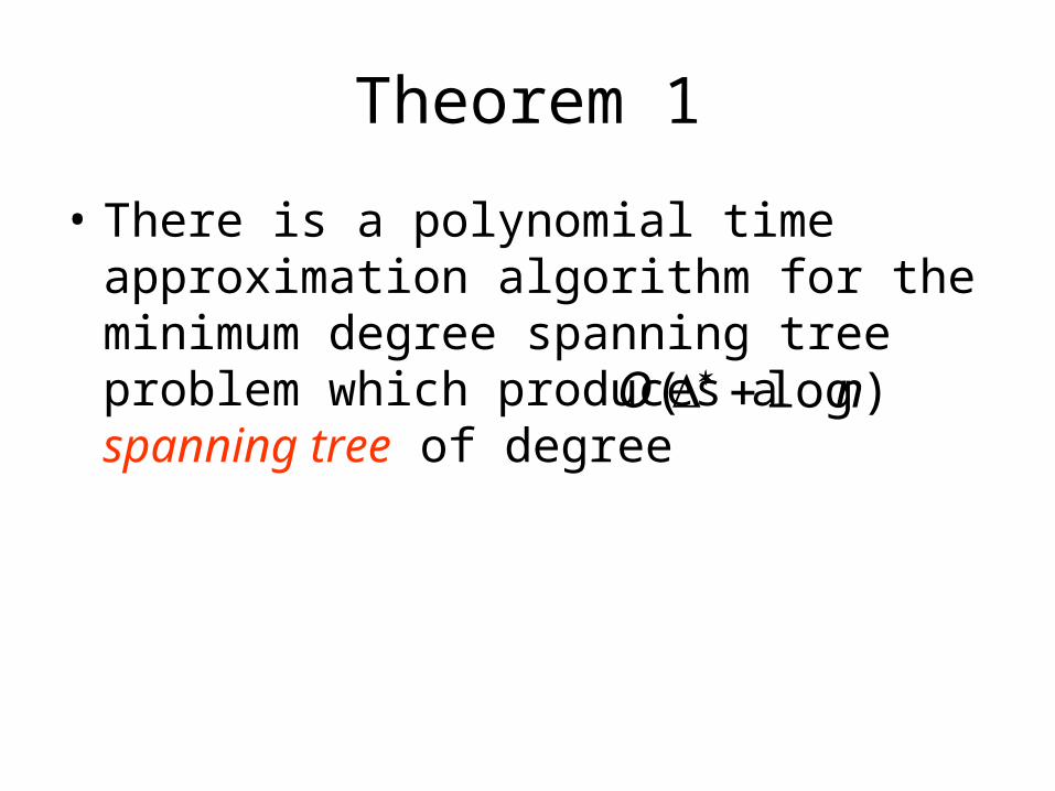
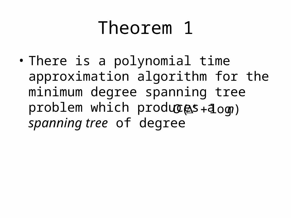
Theorem 1
• There is a polynomial time approximation algorithm for the minimum degree spanning tree problem which produces a spanning tree of degree )log( nO
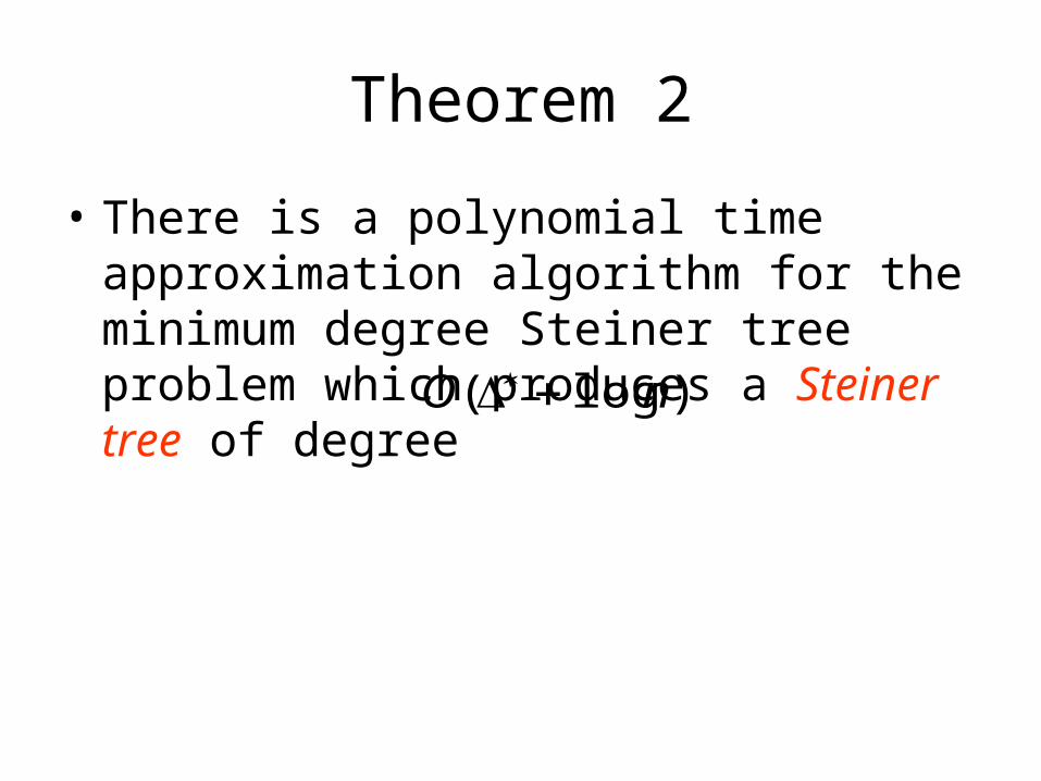
Theorem 2
• There is a polynomial time approximation algorithm for the minimum degree Steiner tree problem which produces a Steiner tree of degree )log( nO
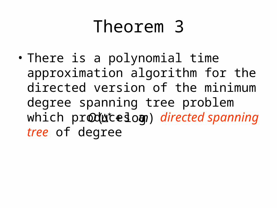
Theorem 3
• There is a polynomial time approximation algorithm for the directed version of the minimum degree spanning tree problem which produces a directed spanning tree of degree )log( nO
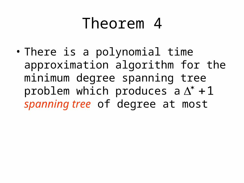
Theorem 4
• There is a polynomial time approximation algorithm for the minimum degree spanning tree problem which produces a spanning tree of degree at most 1

A Simple Approximation Algorithm

Improvement
• :the degree of vertex u in T
• If
we now introduce an “improvement” in T by adding the edge and deleting one of the edge in C incident to
)(u
2))(),(max()( vuw
),( vuw

Example
3
<=211
2
<=2
G T
Locally Optimal Tree
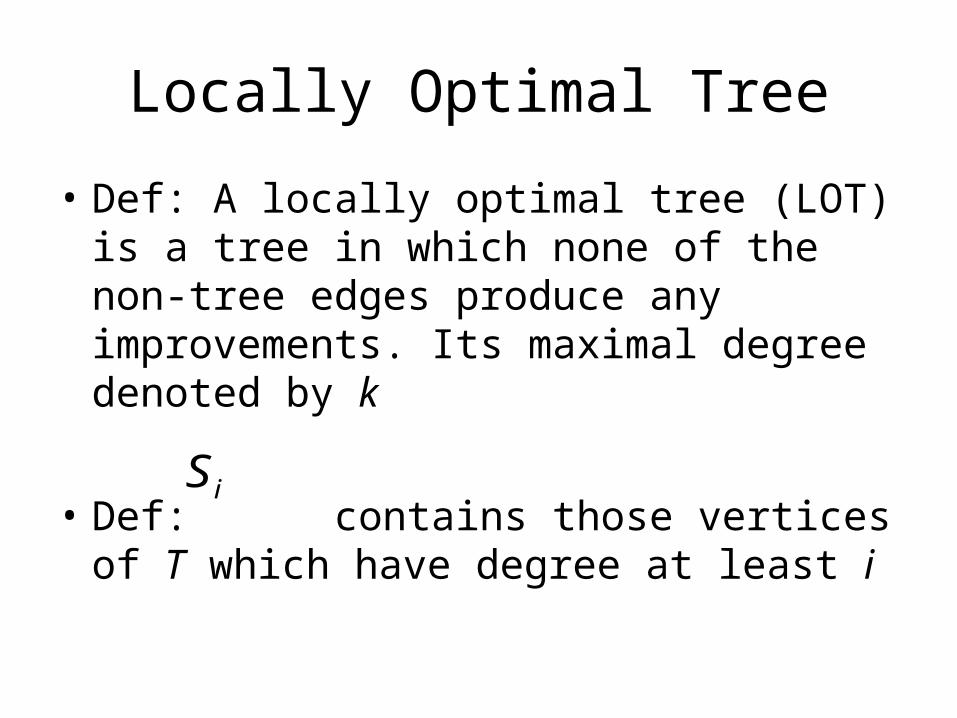
• Def: A locally optimal tree (LOT) is a tree in which none of the non-tree edges produce any improvements. Its maximal degree denoted by k
• Def: contains those vertices of T which have degree at least i
iS

Theorem
• For any b>1, the maximal degree k of a locally optimal tree T is less than
Hence, k = nb blog
)log( nO
Proof
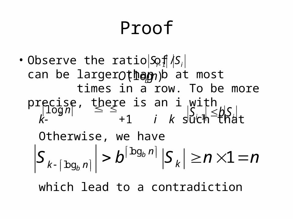
• Observe the ratio of can be larger than b at most times in a row. To be more precise, there is an i with
k- +1 i k such that
Otherwise, we have
which lead to a contradiction
ii SS /1
)(log nO b
nblog ii SbS 1
log
log 1b
b
nkk nS b S n n
Proof
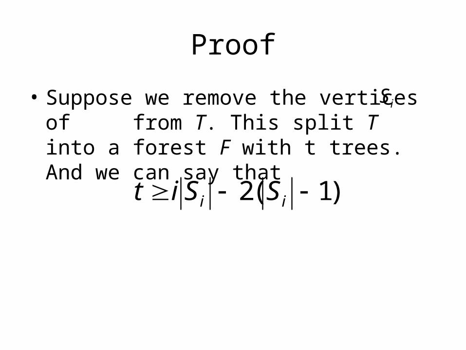
• Suppose we remove the vertices of from T. This split T into a forest F with t trees. And we can say that
iS
)1(2 ii SSit

Proof
• Now, we can say the average degree of vertices in in any spanning tree of G is at least
1iS
1
1
i
i
S
St
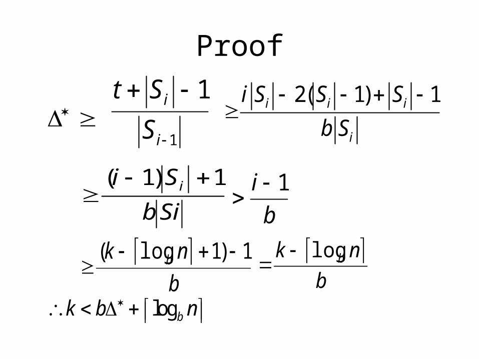
Proof
1
1
i
i
S
St
Sib
Si i 1)1(
2( 1) 1 i i i
i
i S S S
b S
b
i 1
b
nk b 1)1log(
b
nk blog
logbk b n
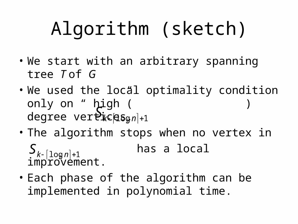
Algorithm (sketch)
• We start with an arbitrary spanning tree T of G
• We used the local optimality condition only on “ high”( ) degree vertices.
• The algorithm stops when no vertex in
has a local improvement.
• Each phase of the algorithm can be implemented in polynomial time.
1log nk bS
1log nk bS
Theorem 1
• There is a polynomial time approximation algorithm for the minimum degree spanning tree problem which produces a spanning tree of degree )log( nO

Idea
• We just need to show that the number of phases is bounded by a polynomial in n.
Proof
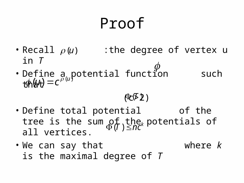
• Recall :the degree of vertex u in T
• Define a potential function such that
(c>2)
• Define total potential of the tree is the sum of the potentials of all vertices.
• We can say that where k is the maximal degree of T
)(u
)()( ucu
)(T
kncT )(

Proof
1 1 1
1 1
1
1 2 2
1
1 2, 2
i i a i b i i a i b
i i a i b i i a i b
i i a i b
i i i
c c c c c c
c c c c c c c
c c c c
c c c c a b
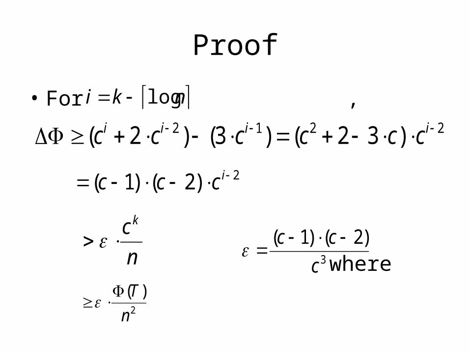
Proof
• For ,
where
2 1 2 2( 2 ) (3 ) ( 2 3 )i i i ic c c c c c nki log
2)2()1( iccc
n
c k
3
)2()1(
c
cc
2
)(
n
T

Proof
• Observe we need phases,the potential reduces by a constant factor.
• On the other hand, k cannot decrease more than n times.
• Hence, bound on the number of phases.
)( 2nO
)( 3nO

The Steiner tree version
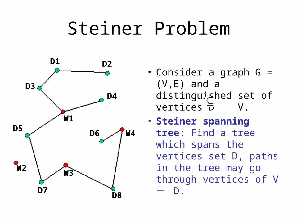
Steiner Problem
• Consider a graph G = (V,E) and a distinguished set of vertices D V.
• Steiner spanning tree: Find a tree which spans the vertices set D, paths in the tree may go through vertices of V - D.
W1
W2W3
W4
D1 D2
D3D4
D5D6
D7D8

Steiner Problem (cont.)
• Minimum Degree Steiner (spanning) Tree– To find a tree of minimum degree, which
spans the set D.– This is a generalization of the [Minimum
Degree Spanning Tree] problem.
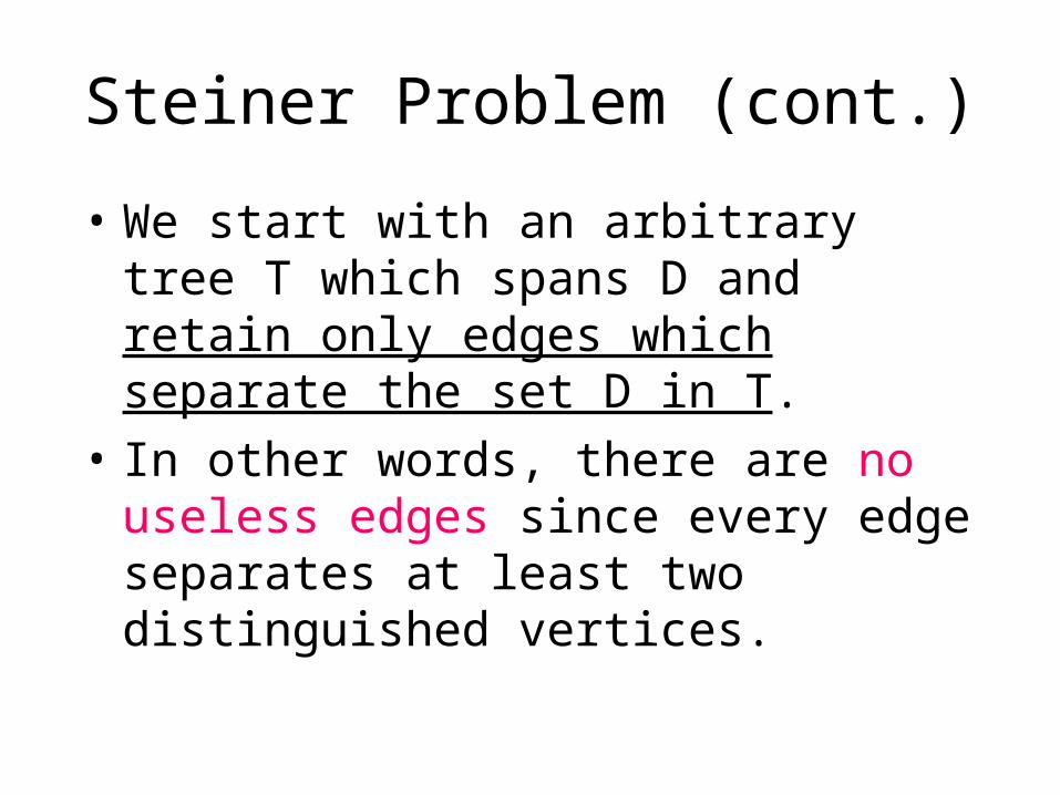
Steiner Problem (cont.)
• We start with an arbitrary tree T which spans D and retain only edges which separate the set D in T.
• In other words, there are no useless edges since every edge separates at least two distinguished vertices.
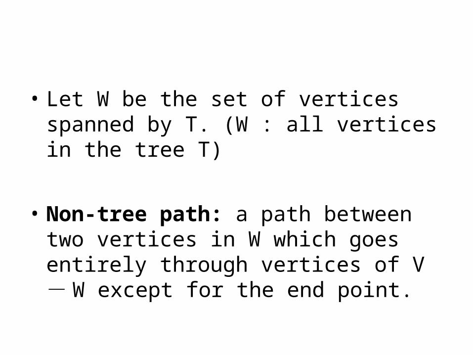
• Let W be the set of vertices spanned by T. (W : all vertices in the tree T)
• Non-tree path: a path between two vertices in W which goes entirely through vertices of V - W except for the end point.
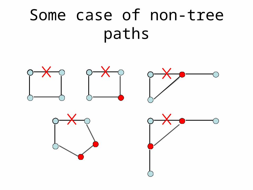
Some case of non-tree paths

Steiner Problem (cont.)
• Pseudo optimal Steiner tree (POST): – Every edge in the tree separates at least two
distinguished vertices.– None of the non-tree paths produce any
improvement for any vertex in Si for i = k- log n⌈ ⌉ , where k denotes the maximal degree of the tree.
– If this property is true for all i, then we call it locally optimal Steiner tree (LOST).
Steiner Problem (cont.)
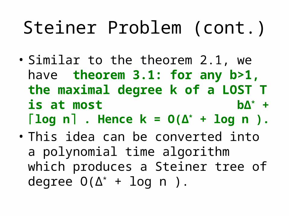
• Similar to the theorem 2.1, we have theorem 3.1: for any b>1, the maximal degree k of a LOST T is at most bΔ* + log n⌈ ⌉ . Hence k = O(Δ* + log n ).
• This idea can be converted into a polynomial time algorithm which produces a Steiner tree of degree O(Δ* + log n ).

Steiner Problem (cont.)
• Theorem 1.2. There is a polynomial time approximation algorithm for the minimum degree Steiner tree problem which produces a Steiner tree of degree O(Δ* + log n ).
Directed spanning trees version
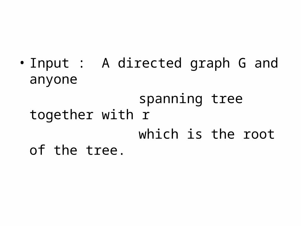
• Input : A directed graph G and anyone
spanning tree together with r
which is the root of the tree.

What is a directed spanning tree ?
• Def : A rooted spanning tree T of G is a
subgraph of G with the following
properties:–T does not contain any cycles.–The outdegree of every vertex except r
is exactly one.–There is a path in T from every vertex to
the root r.
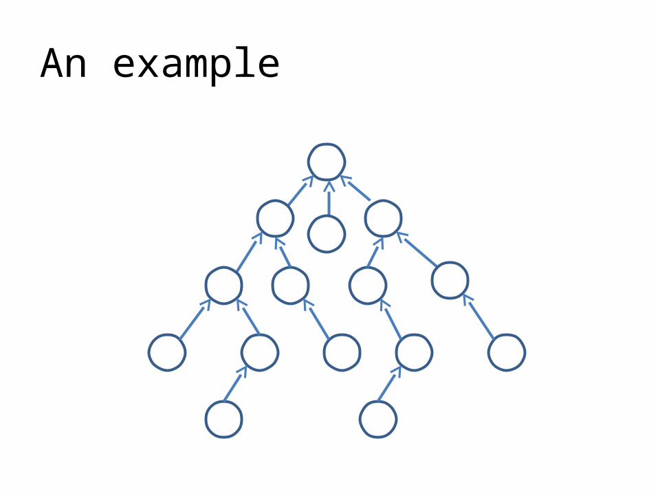
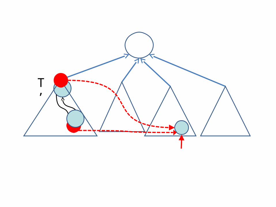
An example
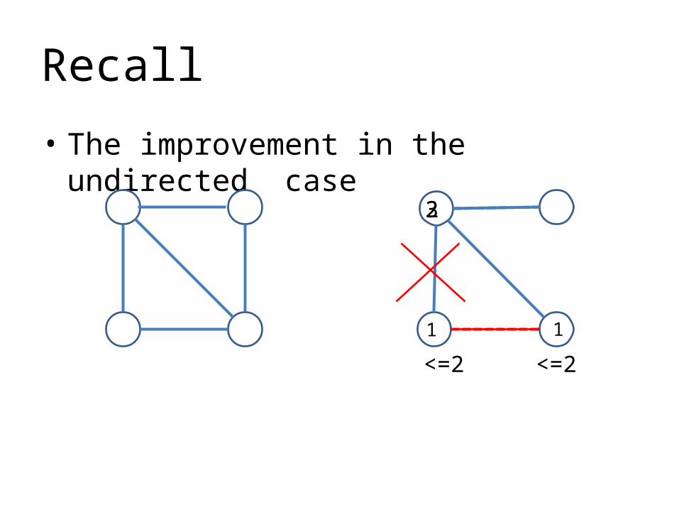
Recall
• The improvement in the undirected case
3
<=2
11
2
<=2
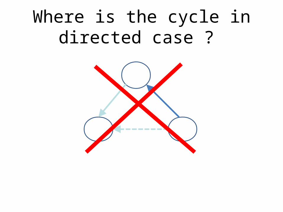
Where is the cycle in directed case ?

New “improvement”
Idea : Consider a vertex v of indegree i.
Try to reduce the indegree of the
vertex by attaching one of the i
subtrees of v to another vertex of
smaller degree.
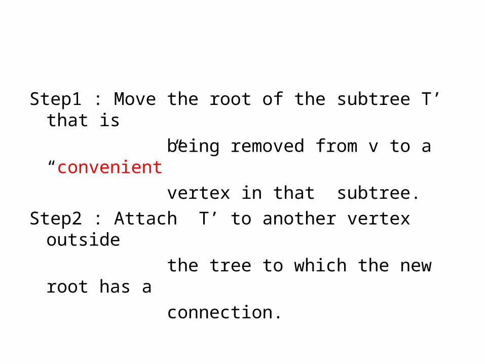
Step1 : Move the root of the subtree T’ that is
being removed from v to a “convenient”
vertex in that subtree.
Step2 : Attach T’ to another vertex outside
the tree to which the new root has a
connection.

What is a convient vertex ?
• The set of convenient vertices are those in the
strongly connected part of the root of T’ in
the graph induced by the vertices of T’ with all
non-tree edges removed from vertices of
degree i – 1 or greater.• We pick a convenient vertex from convenient
set
T’
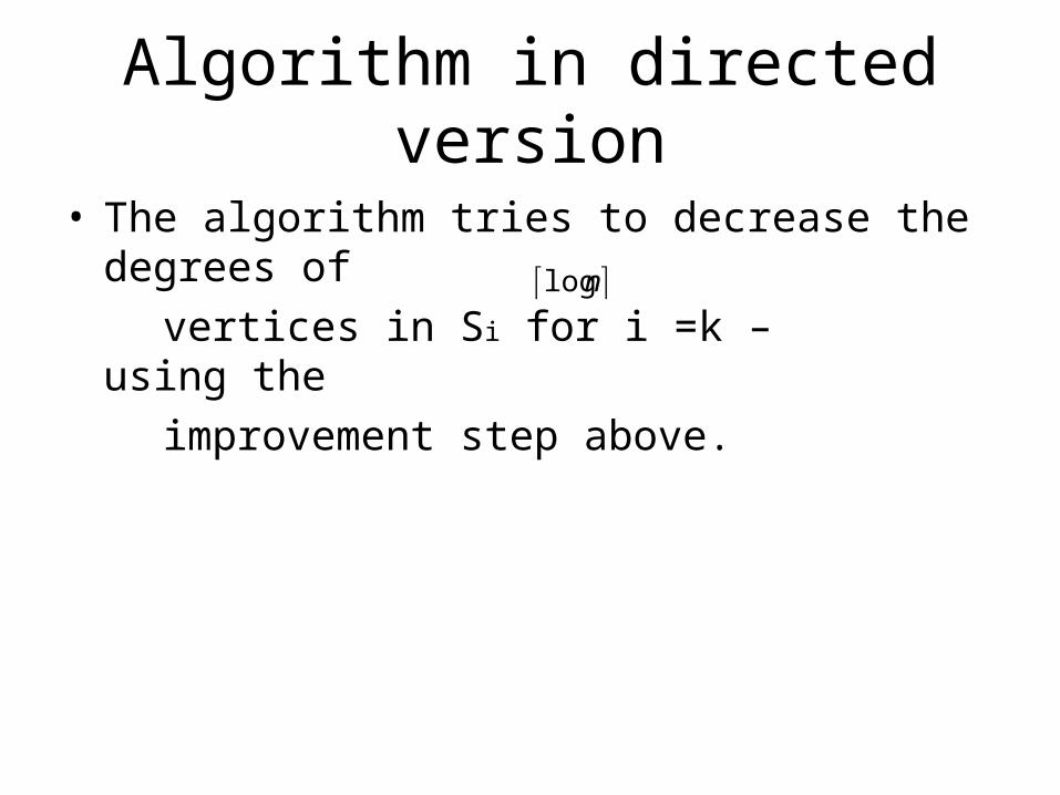
Algorithm in directed version
• The algorithm tries to decrease the degrees of
vertices in Si for i =k – using the
improvement step above. nlog
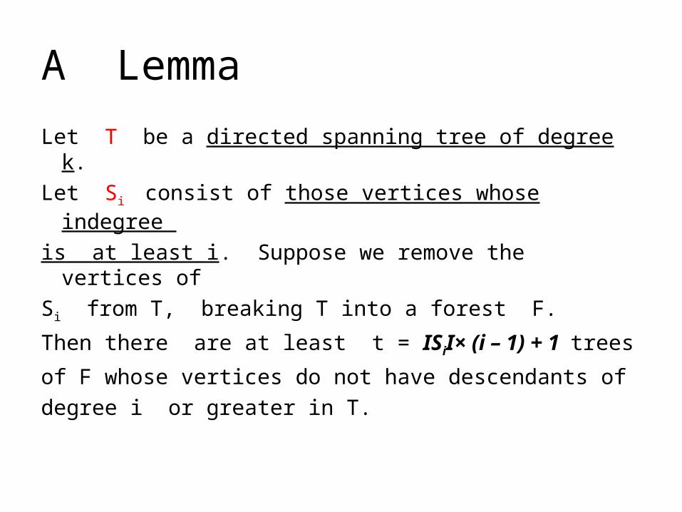
A Lemma
Let T be a directed spanning tree of degree k.
Let Si consist of those vertices whose indegree
is at least i. Suppose we remove the vertices of
Si from T, breaking T into a forest F.
Then there are at least t = ISiI× (i – 1) + 1 trees
of F whose vertices do not have descendants of
degree i or greater in T.
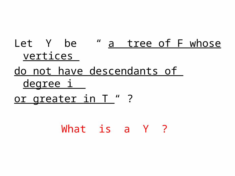
Let Y be “ a tree of F whose vertices
do not have descendants of degree i
or greater in T “ ?
What is a Y ?
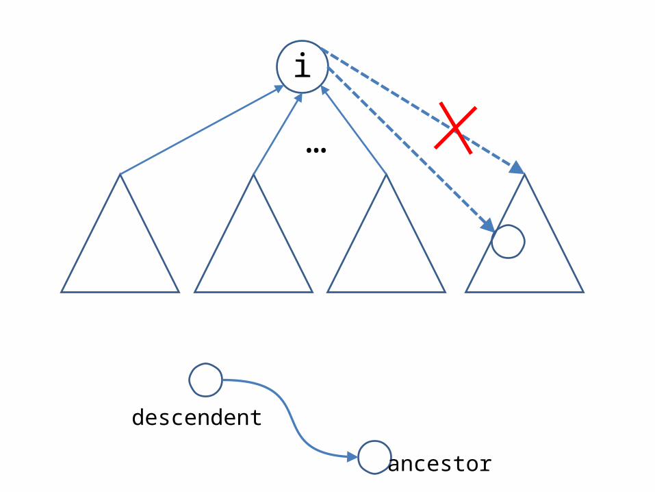
i
descendent
ancestor
…

Why ISiI× (i – 1) + 1 ?
• We use induction on the size of |Si|
– Basis : if |Si| =1, then there are (i-1) +1 = i subtrees like Y (o.k)
Note : Each addition of a vertex to the set S i
can remove at most one tree from the
set of candidate trees, but adds at
least i more.
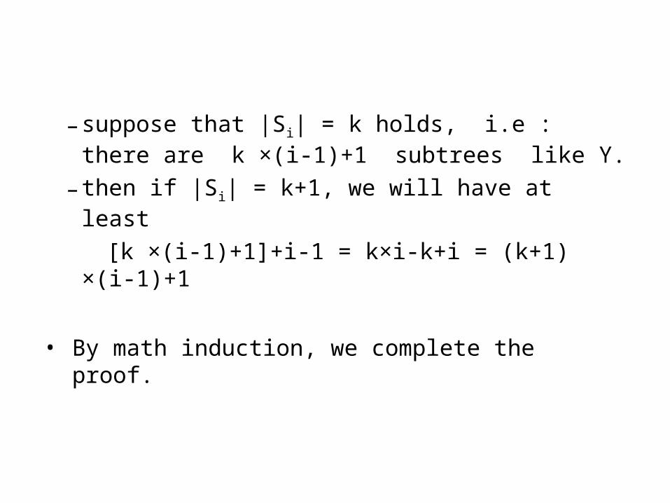
– suppose that |Si| = k holds, i.e : there are k ×(i-1)+1 subtrees like Y.
– then if |Si| = k+1, we will have at least
[k ×(i-1)+1]+i-1 = k×i-k+i = (k+1) ×(i-1)+1
• By math induction, we complete the proof.
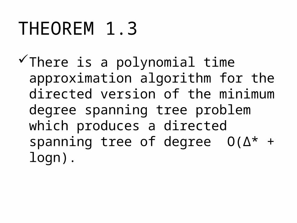
THEOREM 1.3
There is a polynomial time approximation algorithm for the directed version of the minimum degree spanning tree problem which produces a directed spanning tree of degree O(∆* + logn).
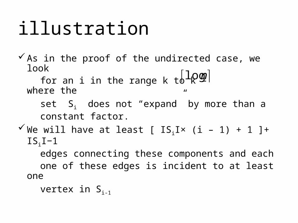
illustration
As in the proof of the undirected case, we look for an i in the range k to k – where the
set Si does not “expand” by more than a constant factor.We will have at least [ ISiI× (i – 1) + 1 ]+ ISiI−1 edges connecting these components and each one of these edges is incident to at least one
vertex in Si-1
nlog

illustration
Hence the average degree of vertices in Si-1 in
any spanning tree of G is at least
The maximal degree ∆* is at least the average
degree of these vertices.
1
1]1)1(|[|
i
ii
S
SiS
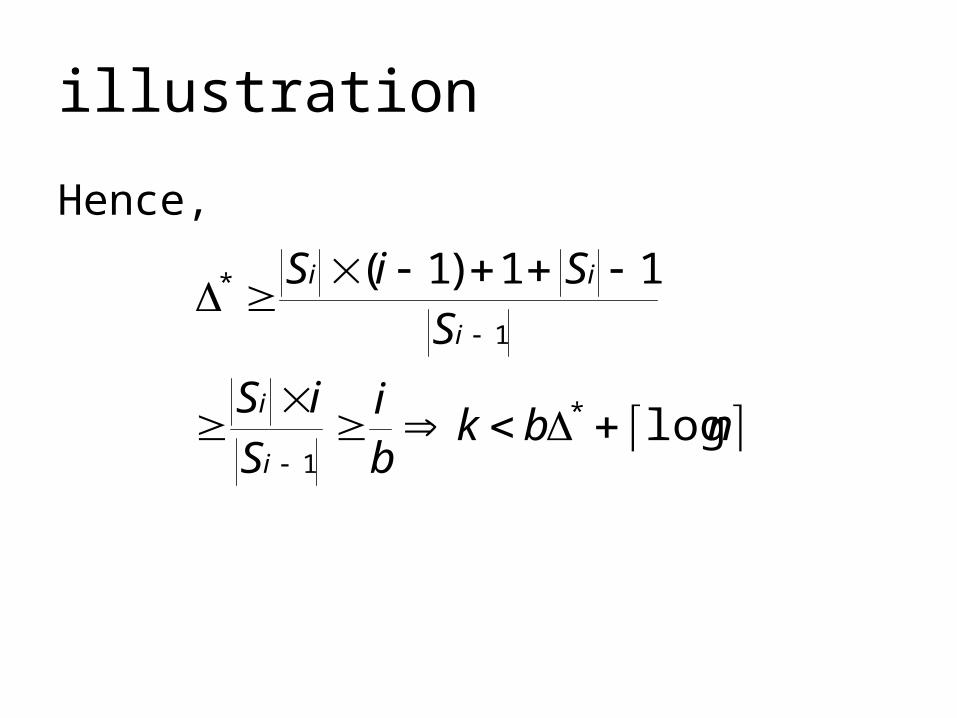
illustration
Hence,
nbkbi
S
iS
S
SiS
i
i
i
ii
log
11)1(
*
1
1
*

The △*+1 algorithm

Definition
k-1k
kk-1
≦k-2
u v
w
≦k-2
k
k-1 k-1
k-1
w
u v
If ρ(u) k – 1, we say that u ≧ blocks w from (u, v).
If neither u nor v blocks w, then w benefits from (u, v).
T
T
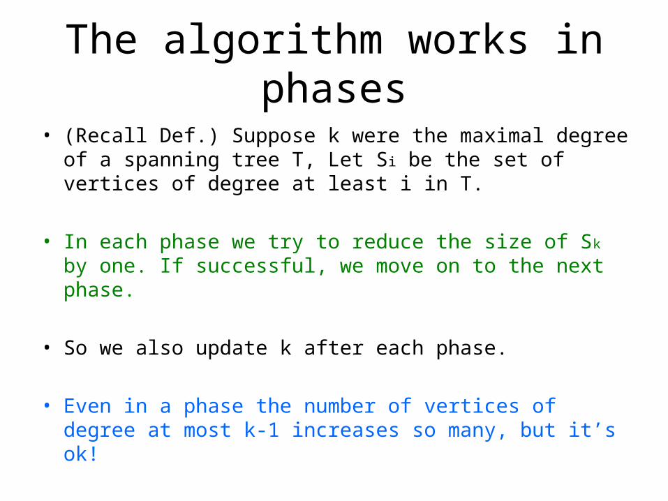
The algorithm works in phases
• (Recall Def.) Suppose k were the maximal degree of a spanning tree T, Let Si be the set of vertices of degree at least i in T.
• In each phase we try to reduce the size of Sk by one. If successful, we move on to the next phase.
• So we also update k after each phase.
• Even in a phase the number of vertices of degree at most k-1 increases so many, but it’s ok!
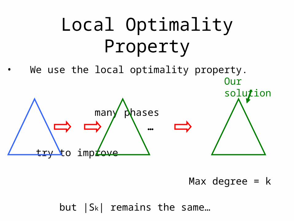
• We use the local optimality property.
many phases
…
try to improve
Max degree = k
but |Sk| remains the same…
Local Optimality Property
Our solution
How many phases?
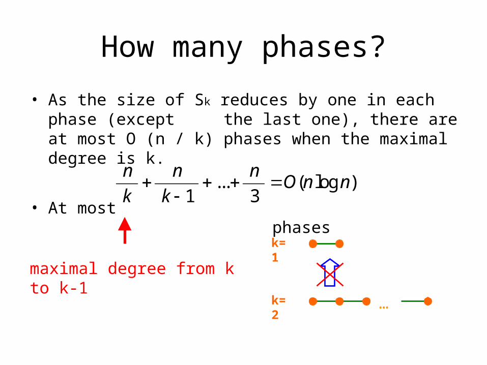
• As the size of Sk reduces by one in each phase (except the last one), there are at most O (n / k) phases when the maximal degree is k.
• At most phases... ( log )1 3
n n nO n n
k k
k=1
k=2
maximal degree from k to k-1
…
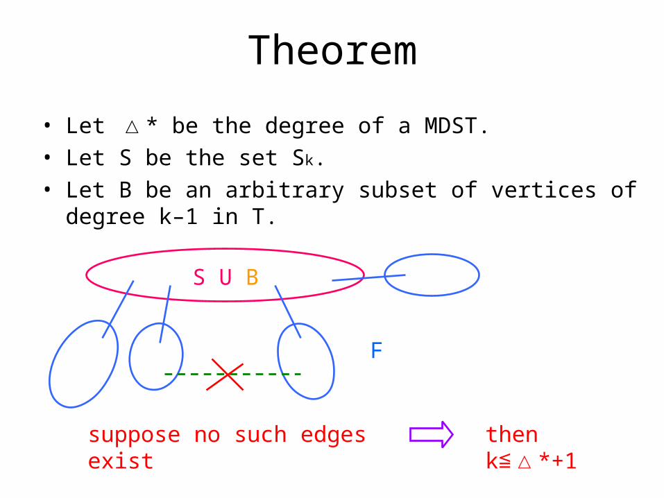
Theorem
• Let * be the degree of a MDST. △• Let S be the set Sk.• Let B be an arbitrary subset of vertices of degree k–1 in T.
S U B
suppose no such edges exist then k *+1≦△
F
Try to prove * something△ ≧
1
1
1
| | 1*
| |
| | 2(| | 1) | | 1
| |
( 1) | | 1
| |
k
k
k k k
k
k
k
t S
S
k S S S
S
k S
S
△
△* ≧ average degree of any subset
we want the vertices of high degree
take Sk
Sk
|F| = t
take S U BS U B
S U B may be either connected or disconnected (Case 1) (Case 2)
( 1) | | 1
| |
k
k
k S
b S
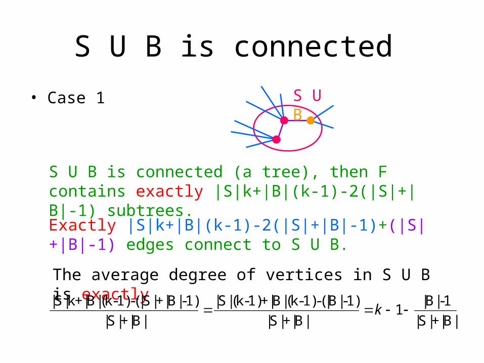
S U B is connected
• Case 1
S U B is connected (a tree), then F contains exactly |S|k+|B|(k-1)-2(|S|+|B|-1) subtrees.
Exactly |S|k+|B|(k-1)-2(|S|+|B|-1)+(|S|+|B|-1) edges connect to S U B.
The average degree of vertices in S U B is exactly
|S|k+|B|(k-1)-(|S|+|B|-1) |S|(k-1)+|B|(k-1)-(|B|-1) |B|-11
|S|+|B| |S|+|B| |S|+|B|k
S U B
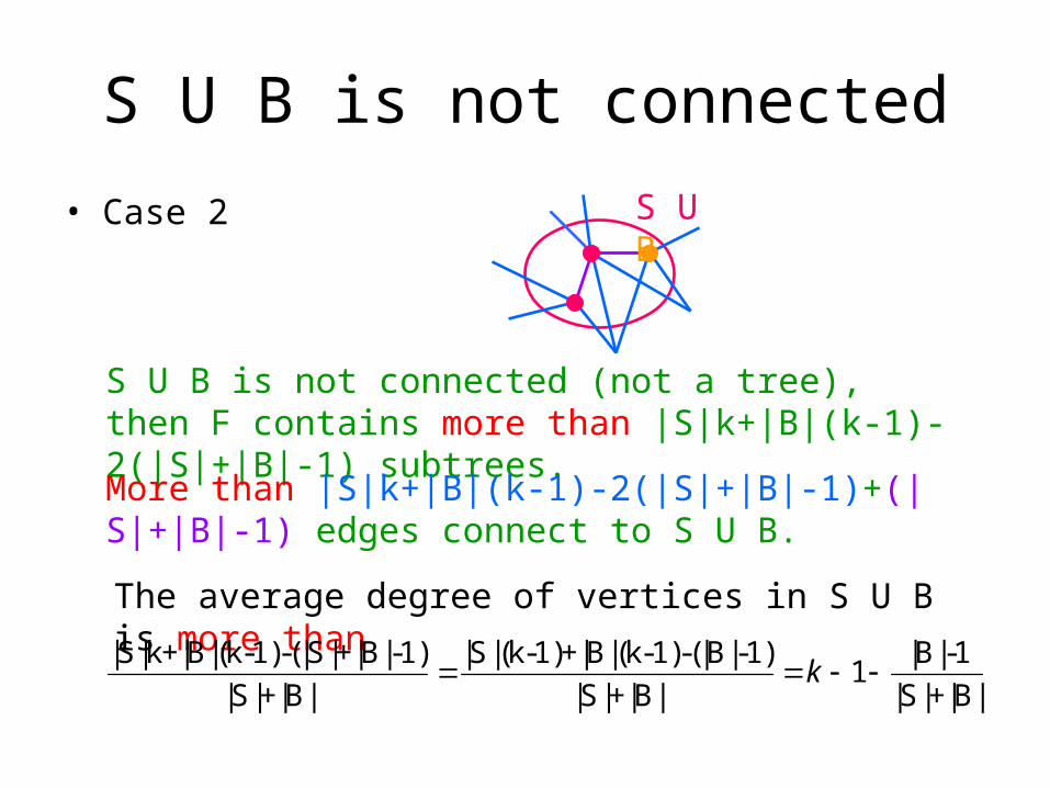
S U B is not connected
• Case 2
S U B is not connected (not a tree), then F contains more than |S|k+|B|(k-1)-2(|S|+|B|-1) subtrees.
More than |S|k+|B|(k-1)-2(|S|+|B|-1)+(|S|+|B|-1) edges connect to S U B.
S U B
The average degree of vertices in S U B is more than
|S|k+|B|(k-1)-(|S|+|B|-1) |S|(k-1)+|B|(k-1)-(|B|-1) |B|-11
|S|+|B| |S|+|B| |S|+|B|k

Finally we proved * k-1△ ≧
• △* ≧ average degree of S U B =
• Therefore * k-1 △ ≧ k *+1≦ △
| | 11
| | | |
Bk
S B
0 1 1* 1 1
|S| 0 |S|
*
k k
k
△
△
• Note : what if |B|=0?
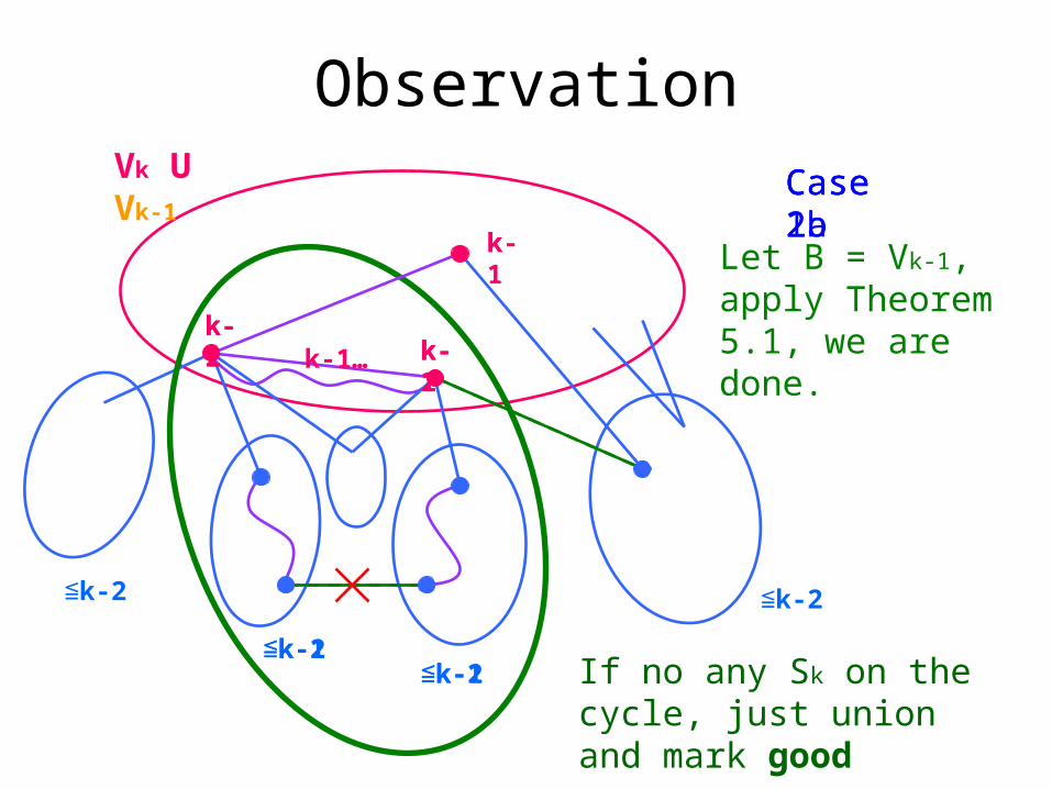
Observation
Let B = Vk-1, apply Theorem 5.1, we are done.
Vk U Vk-1
≦k-2
≦k-2
≦k-2
≦k-2
If no any Sk on the cycle, just union and mark good
kk
k-1k-1k-2
kk-1
Case 1Case 2aCase 2b
k-2k-1…
≦k-1≦k-1

Algorithm• Step 1. Given a SPT (the degree of all vertices is known),
remove Vk U Vk-1 (marked as bad) from T and mark all the connected components as good.
Vk U Vk-1
F
≦k-2≦k-2 ≦k-2
good
bad
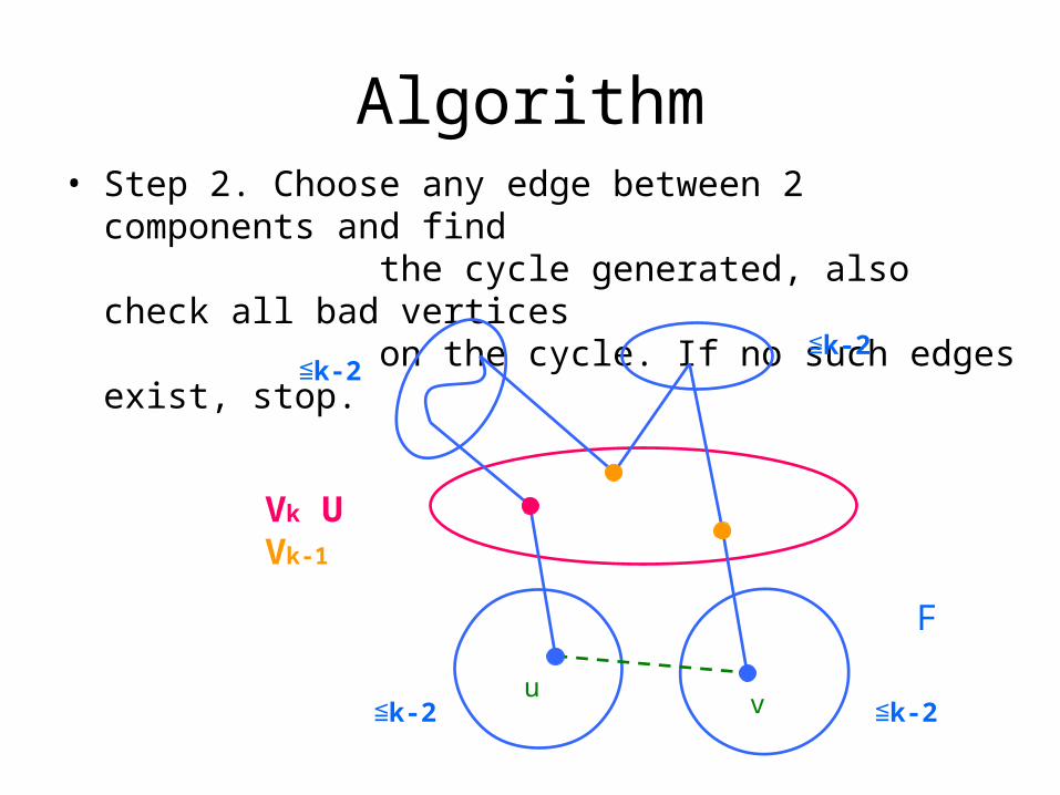
Algorithm• Step 2. Choose any edge between 2 components and find
the cycle generated, also check all bad vertices on the cycle. If no such edges exist, stop.
Vk U Vk-1
F
uv≦k-2
≦k-2
≦k-2
≦k-2
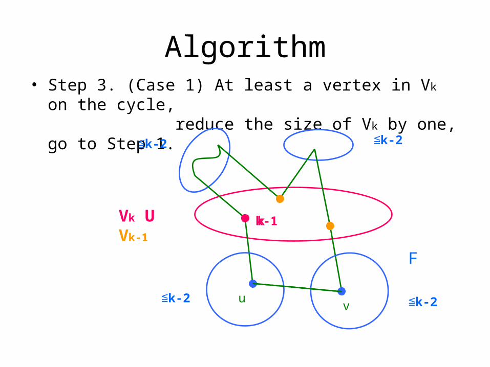
Algorithm• Step 3. (Case 1) At least a vertex in Vk on the cycle,
reduce the size of Vk by one, go to Step 1.
Vk U Vk-1
F
uv
≦k-2
≦k-2 ≦k-2
≦k-2
kk-1
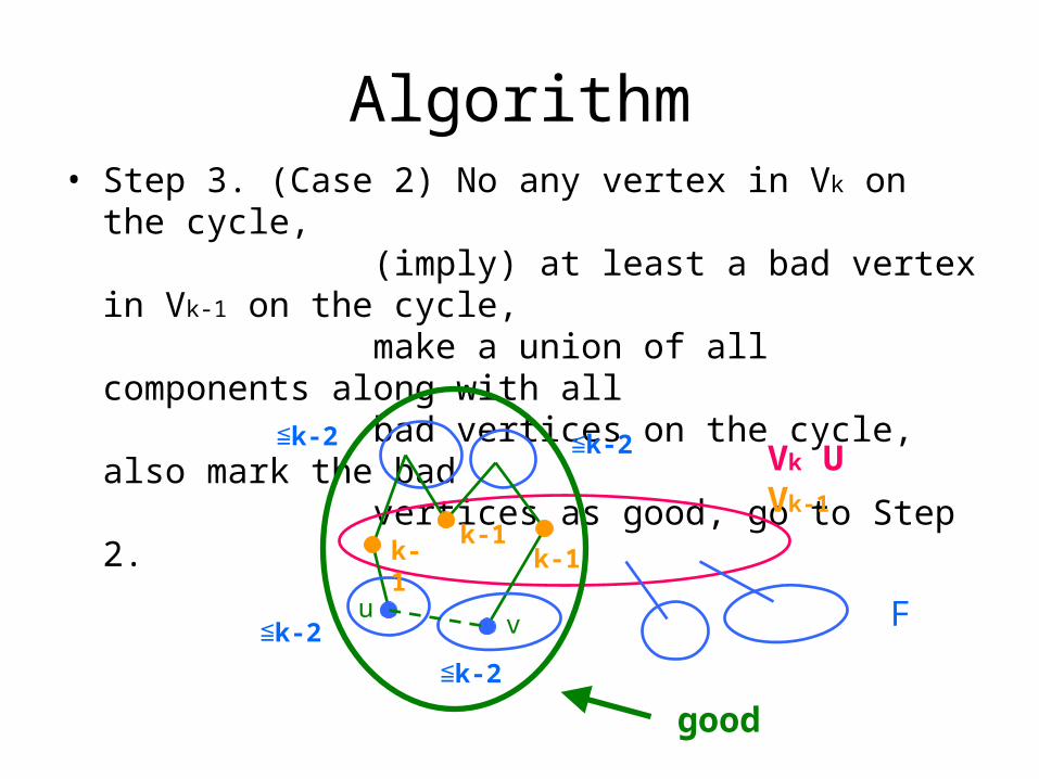
Algorithm• Step 3. (Case 2) No any vertex in Vk on the cycle,
(imply) at least a bad vertex in Vk-1 on the cycle, make a union of all components along with all bad vertices on the cycle, also mark the bad vertices as good, go to Step 2.
Vk U Vk-1
Fuv≦k-2
≦k-2 ≦k-2
≦k-2
k-1k-1 k-1
good
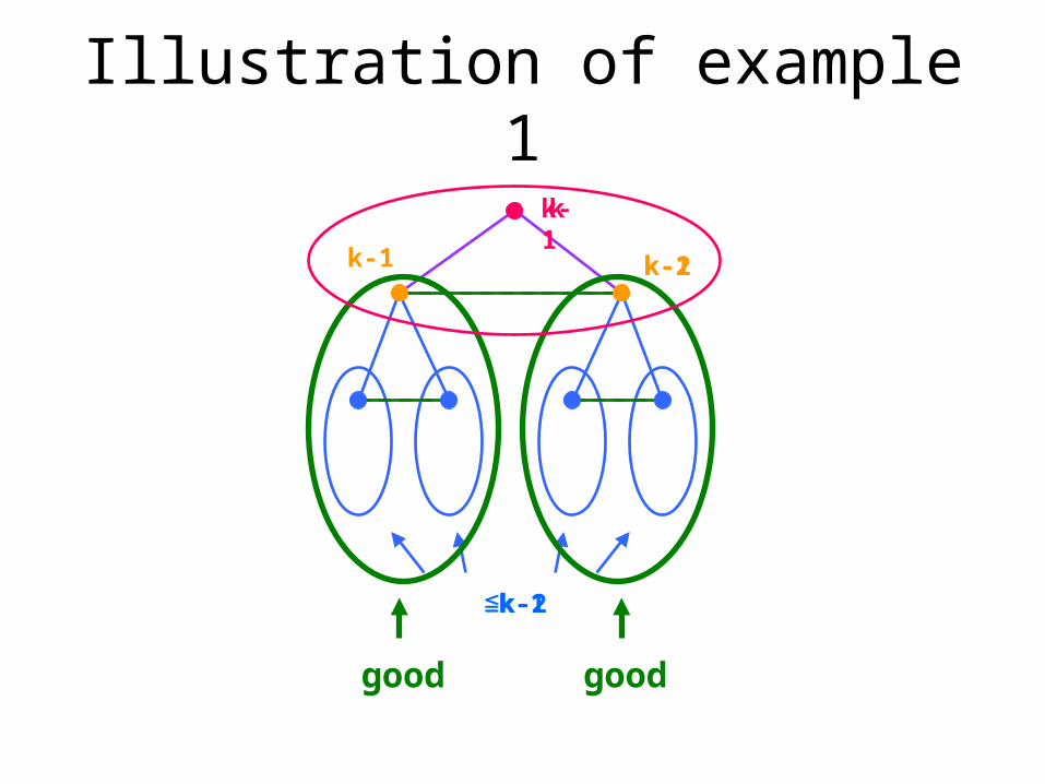
Illustration of example 1
≦k-2
k
k-1k-1
good good
k-2
≦k-1
k-1
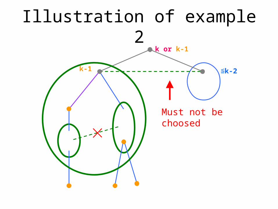
Illustration of example 2
k or k-1
k-1 ≦k-2
Must not be choosed
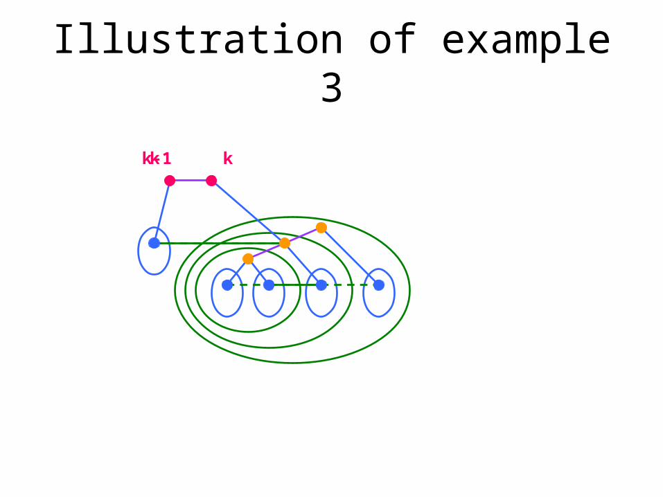
Illustration of example 3
k-1k k
Time analysis
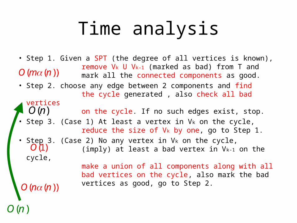
• Step 1. Given a SPT (the degree of all vertices is known), remove Vk U Vk-1 (marked as bad) from T and mark all the connected components as good.
• Step 2. choose any edge between 2 components and find
the cycle generated , also check all bad vertices on the cycle. If no such edges exist, stop.
• Step 3. (Case 1) At least a vertex in Vk on the cycle, reduce the size of Vk by one, go to Step 1.
• Step 3. (Case 2) No any vertex in Vk on the cycle, (imply) at least a bad vertex in Vk-1 on the cycle, make a union of all components along with all bad vertices on the cycle, also mark the bad vertices as good, go to Step 2.
( ( ))O m n
(1)O
( ( ))O n n
)(nO
( )O n