approximation ii
DESCRIPTION
Approximation AlgorithmTRANSCRIPT
LP-Based Algorithms
Introduction
A large fraction of the theory of approximation algorithms is built
around linear programming (LP).
We will review some key concepts from this theory.
We will introduce the two fundamental algorithm design techniques of
rounding and the primal-dual schema, as well as the method of dual
fitting.
3
Linear programming
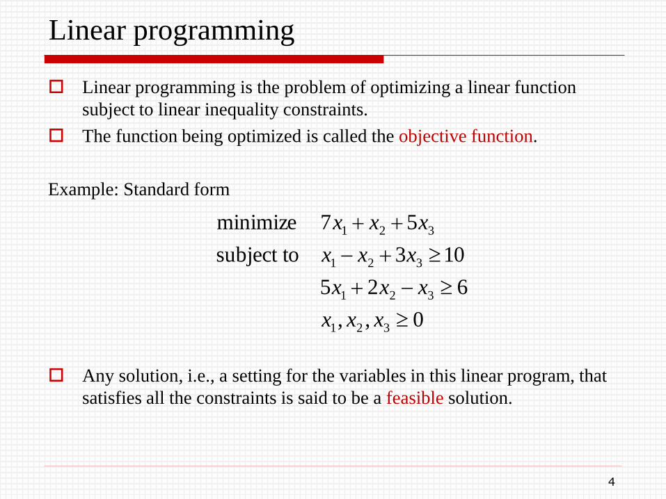
Linear programming is the problem of optimizing a linear function
subject to linear inequality constraints.
The function being optimized is called the objective function.
Example: Standard form
Any solution, i.e., a setting for the variables in this linear program, that
satisfies all the constraints is said to be a feasible solution.
0,,
625
103subject to
57minimize
321
321
321
321
xxx
xxx
xxx
xxx
4
Upper bound
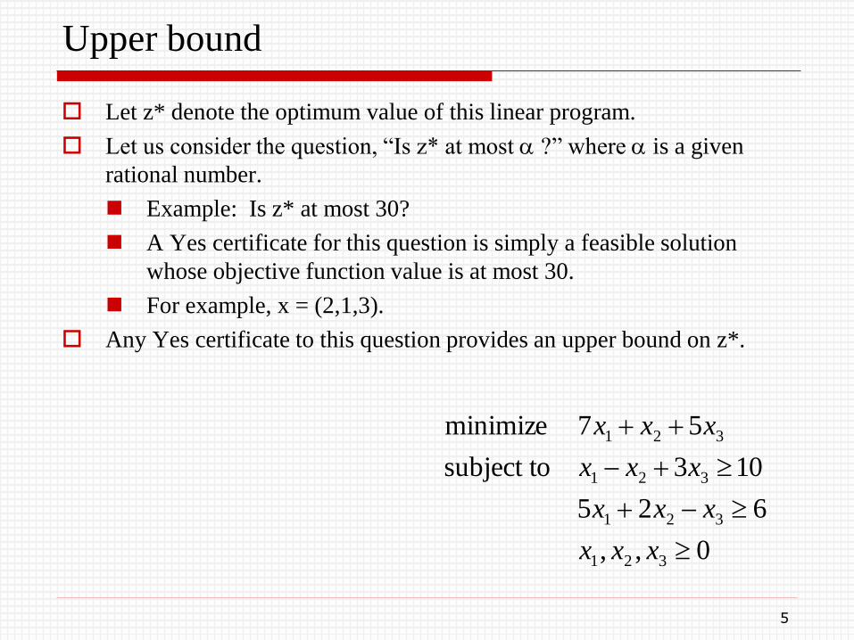
Let z* denote the optimum value of this linear program.
Let us consider the question, “Is z* at most ?” where is a given
rational number.
Example: Is z* at most 30?
A Yes certificate for this question is simply a feasible solution
whose objective function value is at most 30.
For example, x = (2,1,3).
Any Yes certificate to this question provides an upper bound on z*.
0,,
625
103subject to
57minimize
321
321
321
321
xxx
xxx
xxx
xxx
5
Lower bound
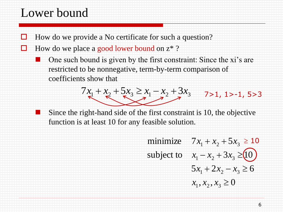
How do we provide a No certificate for such a question?
How do we place a good lower bound on z* ?
One such bound is given by the first constraint: Since the xi’s are
restricted to be nonnegative, term-by-term comparison of
coefficients show that
Since the right-hand side of the first constraint is 10, the objective
function is at least 10 for any feasible solution.
0,,
625
103subject to
57minimize
321
321
321
321
xxx
xxx
xxx
xxx
321321 357 xxxxxx
6
7>1, 1>-1, 5>3
10
Better lower bound
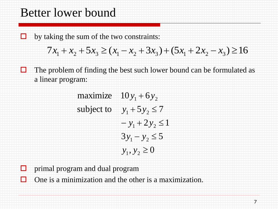
by taking the sum of the two constraints:
The problem of finding the best such lower bound can be formulated as
a linear program:
primal program and dual program
One is a minimization and the other is a maximization.
16)25()3(57 321321321 xxxxxxxxx
0,
53
12
75subject to
610maximize
21
21
21
21
21
yy
yy
yy
yy
yy
7
Primal and Dual
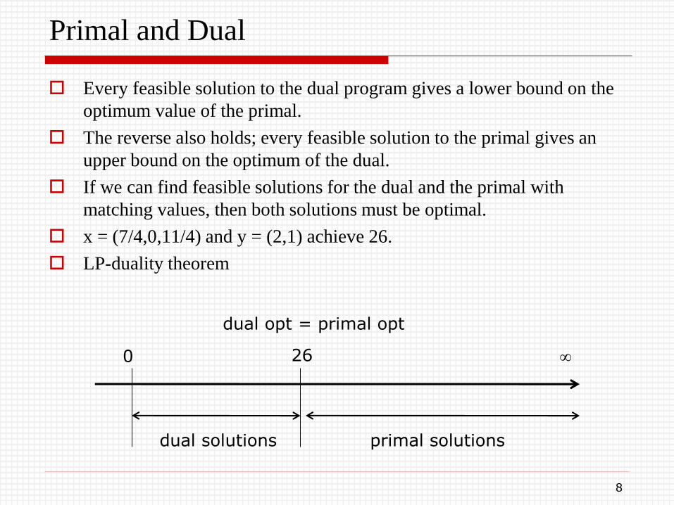
Every feasible solution to the dual program gives a lower bound on the
optimum value of the primal.
The reverse also holds; every feasible solution to the primal gives an
upper bound on the optimum of the dual.
If we can find feasible solutions for the dual and the primal with
matching values, then both solutions must be optimal.
x = (7/4,0,11/4) and y = (2,1) achieve 26.
LP-duality theorem
0 26
dual opt = primal opt
dual solutions primal solutions
8

Primal program
Minimization problem
njx
mibxa
xc
j
n
j
ijij
n
j
jj
,...,10
,...,1subject to
minimize
1
1
9
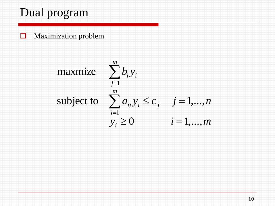
Dual program
Maximization problem
miy
njcya
yb
i
m
i
jiij
m
j
ii
,...,10
,...,1subject to
maxmize
1
1
10
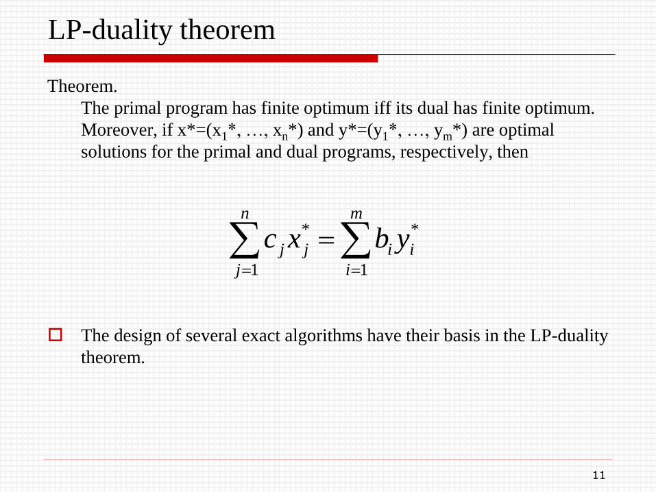
LP-duality theorem
Theorem.
The primal program has finite optimum iff its dual has finite optimum.
Moreover, if x*=(x1*, …, xn*) and y*=(y1*, …, ym*) are optimal
solutions for the primal and dual programs, respectively, then
The design of several exact algorithms have their basis in the LP-duality
theorem.
m
i
ii
n
j
jj ybxc1
*
1
*
11
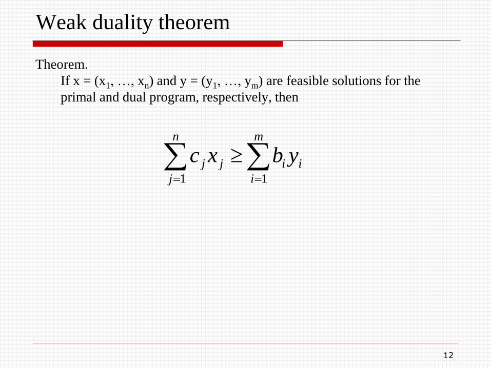
Weak duality theorem
Theorem.
If x = (x1, …, xn) and y = (y1, …, ym) are feasible solutions for the
primal and dual program, respectively, then
m
i
ii
n
j
jj ybxc11
12
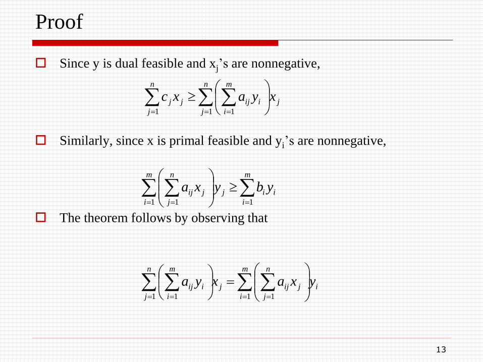
Proof
Since y is dual feasible and xj’s are nonnegative,
Similarly, since x is primal feasible and yi’s are nonnegative,
The theorem follows by observing that
i
m
i
n
j
jijj
n
j
m
i
iij yxaxya
1 11 1
m
i
ii
m
i
j
n
j
jij ybyxa11 1
n
j
j
m
i
iij
n
j
jj xyaxc1 11
13
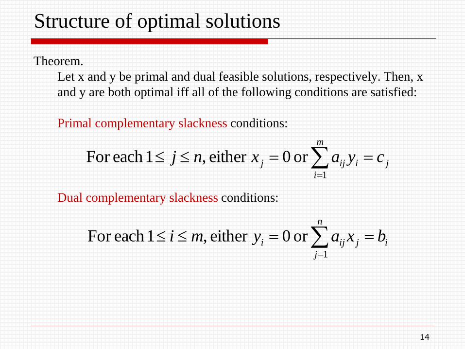
Structure of optimal solutions
Theorem.
Let x and y be primal and dual feasible solutions, respectively. Then, x
and y are both optimal iff all of the following conditions are satisfied:
Primal complementary slackness conditions:
Dual complementary slackness conditions:
j
m
i
iijj cyaxnj 1
or 0either ,1each For
i
n
j
jiji bxaymi 1
or 0either ,1each For
14
Usefulness of LP
Many combinatorial optimization problems can be stated as integer
programs.
Once this is done, the linear relaxation of this program provides a
natural way of lower bounding the cost of the optimal solution.
This is a key step in the design of an approximation algorithm.
Also, in analyzing combinatorially obtained approximation algorithms,
LP-duality theory has been useful, using the method of dual fitting.
15
Two fundamental algorithm design techniques
1. Rounding
Solve the LP and then convert the fractional solution obtained into
an integral solution, trying to ensure that in the process the cost
does not increase much.
The approximation guarantee is established by comparing the cost
of integral and fractional solutions.
2. Primal-dual schema
Use the dual of the LP-relaxation.
Let us call the LP-relaxation the primal program.
Under this schema, an integral solution to the primal program and a
feasible solution to the dual program are constructed iteratively.
The approximation guarantee is established by comparing the two
solutions.
16
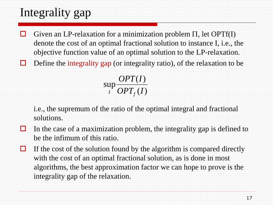
Integrality gap
Given an LP-relaxation for a minimization problem , let OPTf(I)
denote the cost of an optimal fractional solution to instance I, i.e., the
objective function value of an optimal solution to the LP-relaxation.
Define the integrality gap (or integrality ratio), of the relaxation to be
i.e., the supremum of the ratio of the optimal integral and fractional
solutions.
In the case of a maximization problem, the integrality gap is defined to
be the infimum of this ratio.
If the cost of the solution found by the algorithm is compared directly
with the cost of an optimal fractional solution, as is done in most
algorithms, the best approximation factor we can hope to prove is the
integrality gap of the relaxation.
17
)(
)(sup
IOPT
IOPT
fI
A comparison of the two techniques
LP-rounding vs Primal-dual schema
For many problems, both techniques have been successful in yielding
algorithms having guarantees essentially equal to the integrality gap of
the relaxation.
The main difference lies in the running times.
An LP-rounding algorithm needs to find an optimal solution to the LP
relaxation. The running time is high.
The primal-dual schema leaves enough room to exploit the special
combinatorial structure of individual problems and is thereby able to
yield algorithms having good running times.
From a practical standpoint, a combinatorial algorithm is more useful,
since it is easier to adapt it to specific applications and fine tune its
performance for specific types of inputs.
18

Set Cover via Dual Fitting
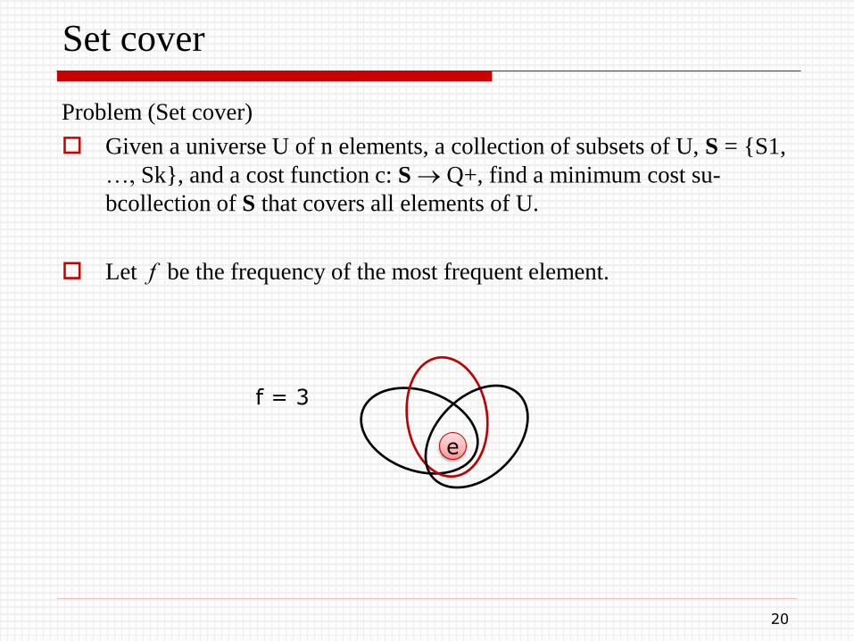
Set cover
Problem (Set cover)
Given a universe U of n elements, a collection of subsets of U, S = {S1,
…, Sk}, and a cost function c: S Q+, find a minimum cost su-
bcollection of S that covers all elements of U.
Let f be the frequency of the most frequent element.
20
e
f = 3
Dual fitting
Outline, assuming a minimization problem:
The basic algorithm is combinatorial.
Using the LP-relaxation of the problem and its dual, one shows that the
primal integral solution found by the algorithm is fully paid for by the
dual computed; however, the dual is infeasible.
By fully paid we mean that the objective function value of the primal
solution found is at most the objective function value of the dual
computed.
The main step in the analysis consists of dividing the dual by a suitable
factor and showing that the shrunk dual is feasible, i.e., it fits into the
given instance.
The shrunk dual is then a lower bound of OPT, and the factor is the
approximation guarantee of the algorithm.
21
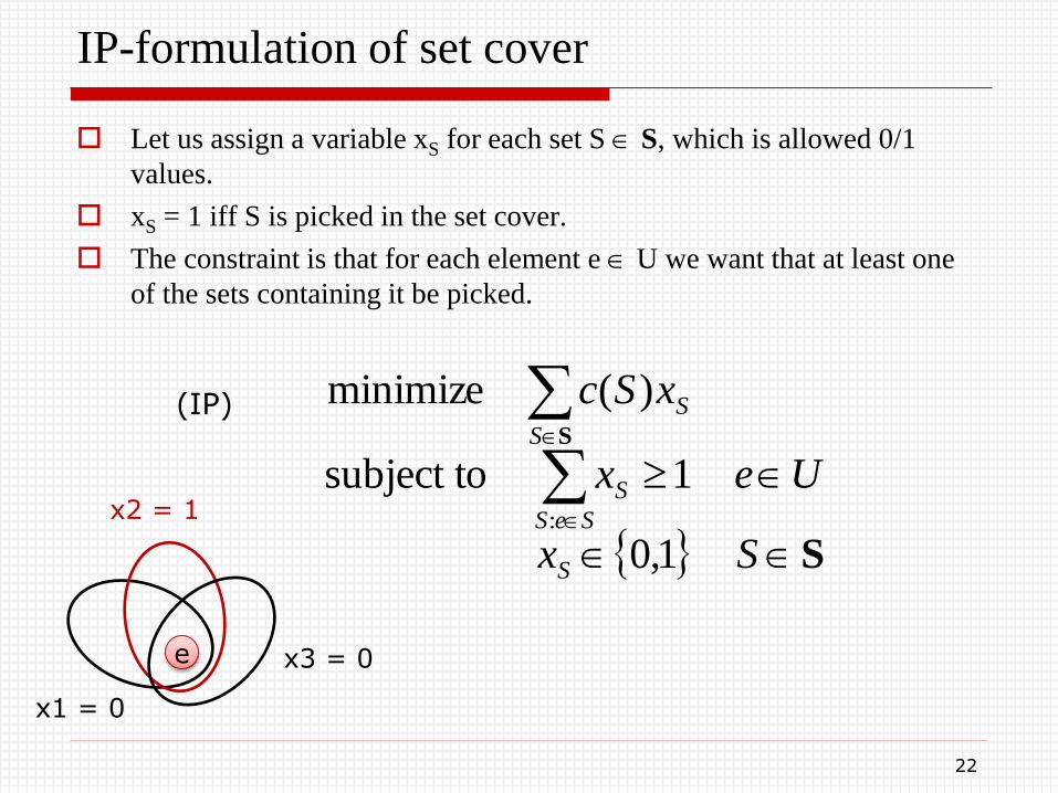
IP-formulation of set cover
Let us assign a variable xS for each set S S, which is allowed 0/1
values.
xS = 1 iff S is picked in the set cover.
The constraint is that for each element e U we want that at least one
of the sets containing it be picked.
S
S
Sx
Uex
xSc
S
SeS
S
S
S
1,0
1subject to
)(minimize
:
e
x1 = 0
x3 = 0
x2 = 1
22
(IP)
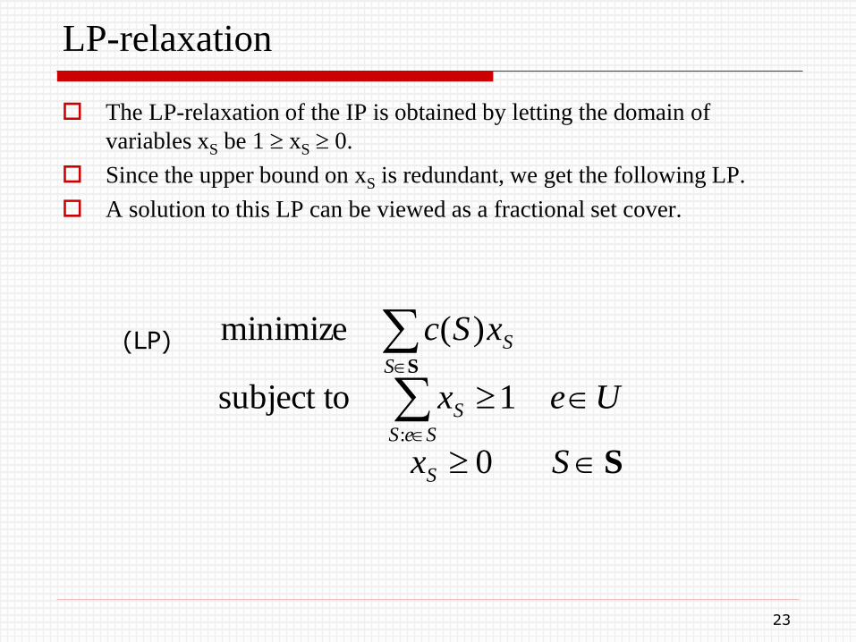
LP-relaxation
The LP-relaxation of the IP is obtained by letting the domain of
variables xS be 1 xS 0.
Since the upper bound on xS is redundant, we get the following LP.
A solution to this LP can be viewed as a fractional set cover.
S
S
Sx
Uex
xSc
S
SeS
S
S
S
0
1subject to
)(minimize
:
23
(LP)
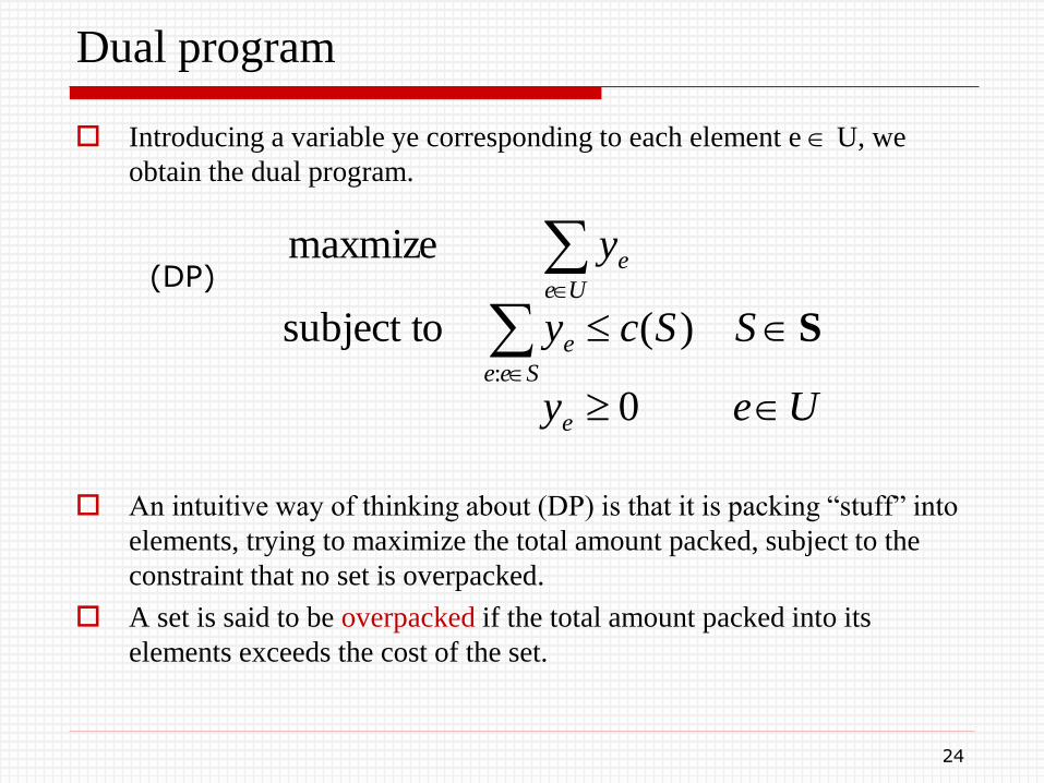
Dual program
Introducing a variable ye corresponding to each element e U, we
obtain the dual program.
An intuitive way of thinking about (DP) is that it is packing “stuff” into
elements, trying to maximize the total amount packed, subject to the
constraint that no set is overpacked.
A set is said to be overpacked if the total amount packed into its
elements exceeds the cost of the set.
Uey
SScy
y
e
See
e
Ue
e
0
)(subject to
maxmize
:
S
24
(DP)
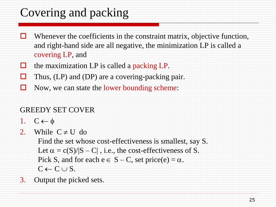
Covering and packing
Whenever the coefficients in the constraint matrix, objective function,
and right-hand side are all negative, the minimization LP is called a
covering LP, and
the maximization LP is called a packing LP.
Thus, (LP) and (DP) are a covering-packing pair.
Now, we can state the lower bounding scheme:
GREEDY SET COVER
1. C
2. While C U do
Find the set whose cost-effectiveness is smallest, say S.
Let = c(S)/|S – C| , i.e., the cost-effectiveness of S.
Pick S, and for each e S – C, set price(e) = .
C C S.
3. Output the picked sets.
25
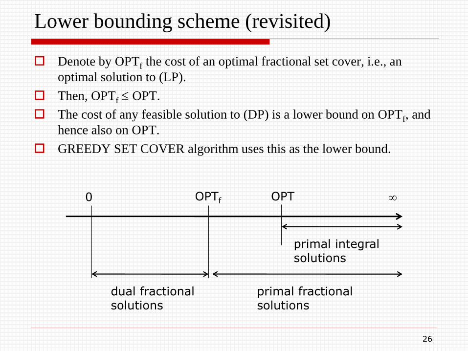
Lower bounding scheme (revisited)
Denote by OPTf the cost of an optimal fractional set cover, i.e., an
optimal solution to (LP).
Then, OPTf OPT.
The cost of any feasible solution to (DP) is a lower bound on OPTf, and
hence also on OPT.
GREEDY SET COVER algorithm uses this as the lower bound.
26
0 OPTf
dual fractionalsolutions
primal fractionalsolutions
OPT
primal integralsolutions
Lower bounding scheme (revisited)
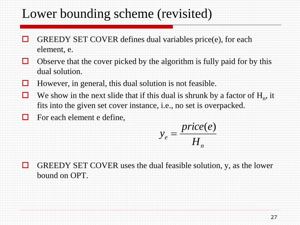
GREEDY SET COVER defines dual variables price(e), for each
element, e.
Observe that the cover picked by the algorithm is fully paid for by this
dual solution.
However, in general, this dual solution is not feasible.
We show in the next slide that if this dual is shrunk by a factor of Hn, it
fits into the given set cover instance, i.e., no set is overpacked.
For each element e define,
GREEDY SET COVER uses the dual feasible solution, y, as the lower
bound on OPT.
27
n
eH
epricey
)(
Lower bounding scheme (revisited)
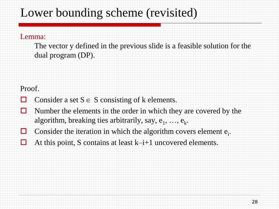
Lemma:
The vector y defined in the previous slide is a feasible solution for the
dual program (DP).
Proof.
Consider a set S S consisting of k elements.
Number the elements in the order in which they are covered by the
algorithm, breaking ties arbitrarily, say, e1, …, ek.
Consider the iteration in which the algorithm covers element ei.
At this point, S contains at least k–i+1 uncovered elements.
28
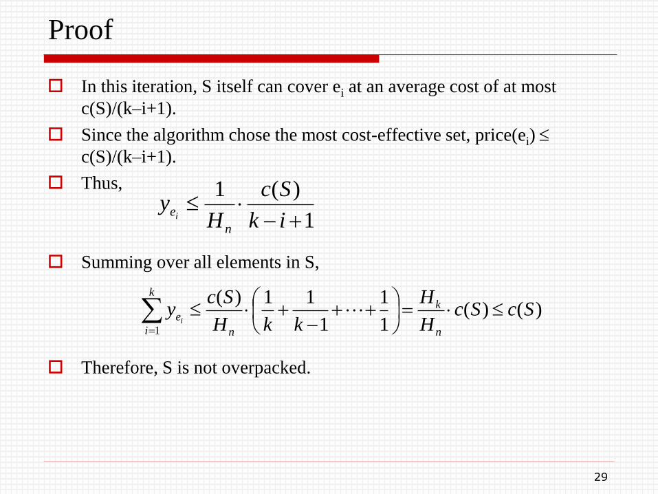
Proof
In this iteration, S itself can cover ei at an average cost of at most
c(S)/(k–i+1).
Since the algorithm chose the most cost-effective set, price(ei)
c(S)/(k–i+1).
Thus,
Summing over all elements in S,
Therefore, S is not overpacked.
29
1
)(1
ik
Sc
Hy
n
ei
)()(1
1
1
11)(
1
ScScH
H
kkH
Scy
n
k
n
k
i
ei
Approximation ratio
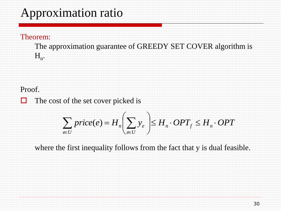
Theorem:
The approximation guarantee of GREEDY SET COVER algorithm is
Hn.
Proof.
The cost of the set cover picked is
where the first inequality follows from the fact that y is dual feasible.
30
OPTHOPTHyHeprice nfn
Ue
en
Ue
)(

Rounding Applied to Set Cover
A simple rounding algorithm
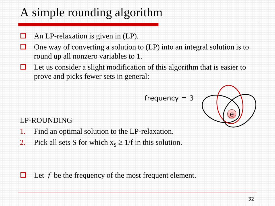
An LP-relaxation is given in (LP).
One way of converting a solution to (LP) into an integral solution is to
round up all nonzero variables to 1.
Let us consider a slight modification of this algorithm that is easier to
prove and picks fewer sets in general:
LP-ROUNDING
1. Find an optimal solution to the LP-relaxation.
2. Pick all sets S for which xS 1/f in this solution.
Let f be the frequency of the most frequent element.
32
e
frequency = 3
Approximation ratio of LP-ROUNDING
Theorem:
LP-ROUNDING algorithm achieves an approximation factor of f for
the set cover problem.
Proof.
Let C be the collection of picked sets.
Consider an arbitrary element e.
Since e is in at most f sets, one of these sets must be picked to the extent
of at least 1/f in the fractional cover.
Thus, e is covered by C, and hence C is a valid set cover.
The rounding process increase xS, for each set S C, by a factor of at
most f.
Therefore, the cost of C is at most f times the cost of the fractional
cover, thereby proving the desired approximation guarantee.
33

Set Cover via the Primal-dual Schema
Overview of the schema
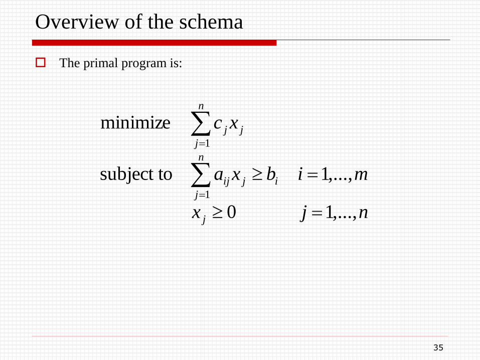
The primal program is:
35
njx
mibxa
xc
j
n
j
ijij
n
j
jj
,...,10
,...,1subject to
minimize
1
1
Overview of the schema
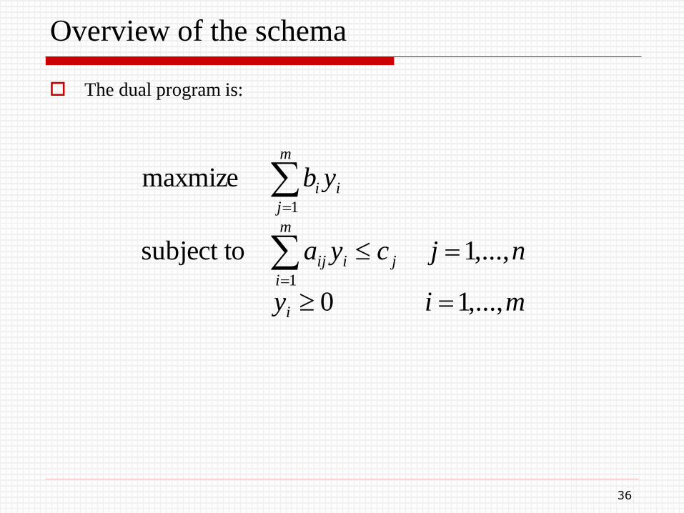
The dual program is:
36
miy
njcya
yb
i
m
i
jiij
m
j
ii
,...,10
,...,1subject to
maxmize
1
1
Overview of the schema
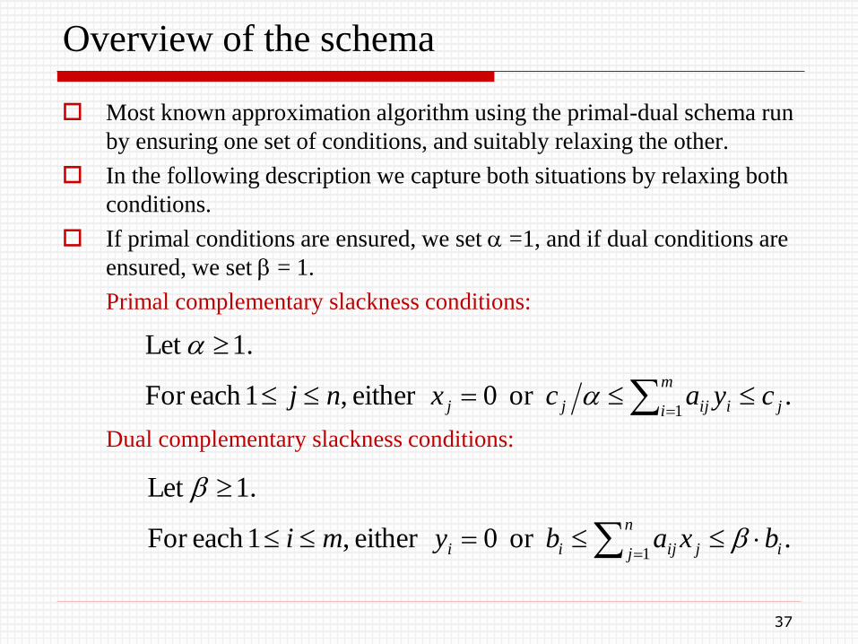
Most known approximation algorithm using the primal-dual schema run
by ensuring one set of conditions, and suitably relaxing the other.
In the following description we capture both situations by relaxing both
conditions.
If primal conditions are ensured, we set =1, and if dual conditions are
ensured, we set = 1.
Primal complementary slackness conditions:
Dual complementary slackness conditions:
37
.or 0either ,1each For
.1Let
1 j
m
i iijjj cyacxnj
.or 0either ,1each For
.1Let
1 i
n
j jijii bxabymi
Overview of the schema
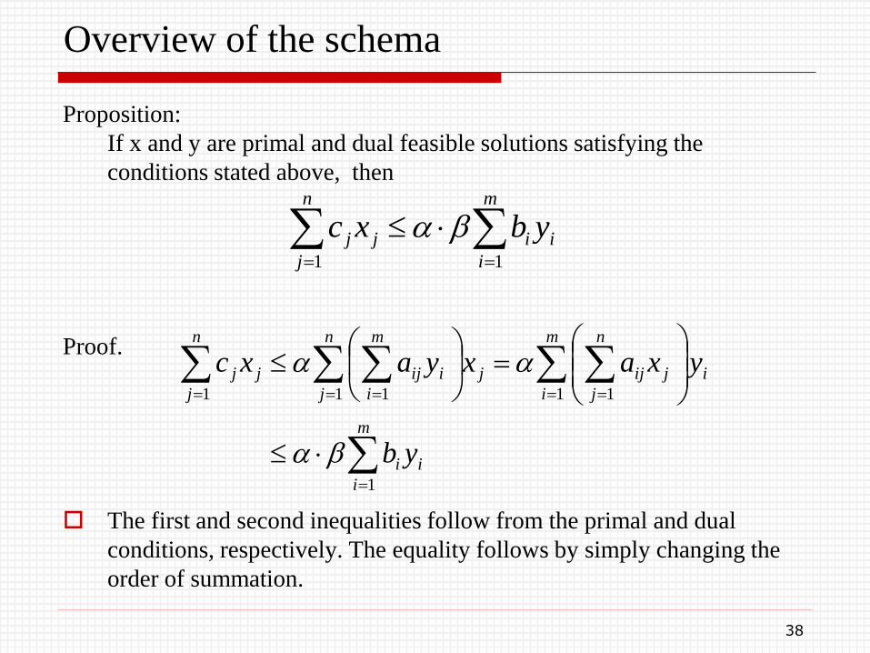
Proposition:
If x and y are primal and dual feasible solutions satisfying the
conditions stated above, then
Proof.
The first and second inequalities follow from the primal and dual
conditions, respectively. The equality follows by simply changing the
order of summation.
38
m
i
ii
n
j
jj ybxc11
m
i
ii
m
i
i
n
j
jij
n
j
j
m
i
iij
n
j
jj
yb
yxaxyaxc
1
1 11 11
Overview of the schema
The algorithm starts with a primal infeasible solution and a dual feasible
solution; these are usually the trivial solutions x = 0 and y = 0.
It iteratively improves the feasibility of the primal solution, and the
optimality of the dual solution, ensuring that in the end a primal feasible
solution is obtained and all conditions are satisfied with a suitable
choice of and .
The primal solution is always extended integrally, thus ensuring that the
final solution is integral.
The current primal solution is used to determine the improvement to the
dual, and vice versa.
Finally, the cost of the dual solution is used as a lower bound on OPT.
By the proposition, the approximation guarantee of the algorithm is .
39
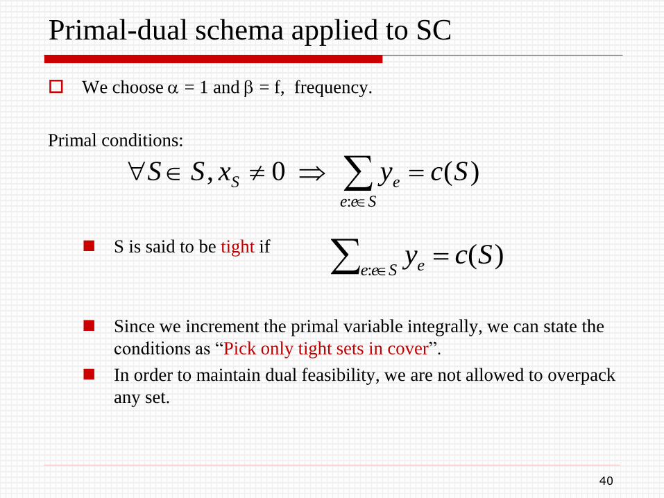
Primal-dual schema applied to SC
We choose = 1 and = f, frequency.
Primal conditions:
S is said to be tight if
Since we increment the primal variable integrally, we can state the
conditions as “Pick only tight sets in cover”.
In order to maintain dual feasibility, we are not allowed to overpack
any set.
40
)(0,:
ScyxSSSee
eS
)(:
ScySee e
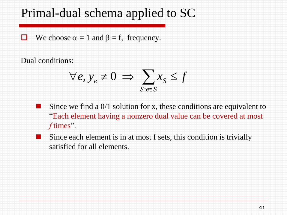
Primal-dual schema applied to SC
We choose = 1 and = f, frequency.
Dual conditions:
Since we find a 0/1 solution for x, these conditions are equivalent to
“Each element having a nonzero dual value can be covered at most
f times”.
Since each element is in at most f sets, this condition is trivially
satisfied for all elements.
41
fxyeSeS
Se :
0,
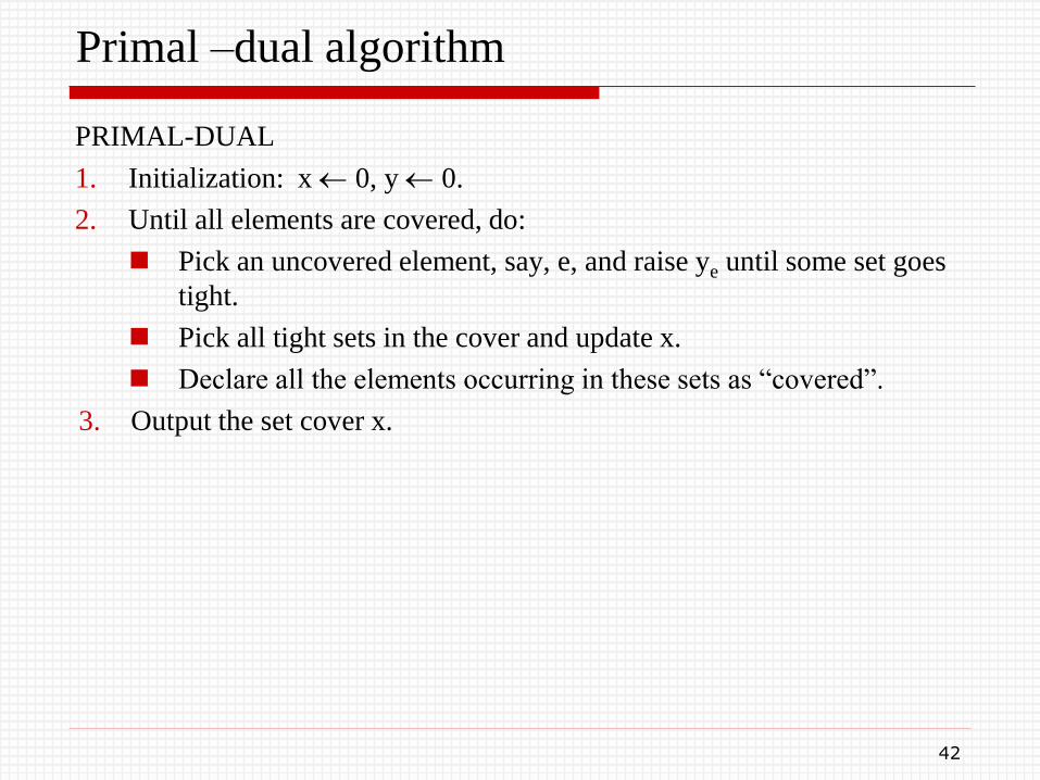
Primal –dual algorithm
PRIMAL-DUAL
1. Initialization: x 0, y 0.
2. Until all elements are covered, do:
Pick an uncovered element, say, e, and raise ye until some set goes
tight.
Pick all tight sets in the cover and update x.
Declare all the elements occurring in these sets as “covered”.
3. Output the set cover x.
42
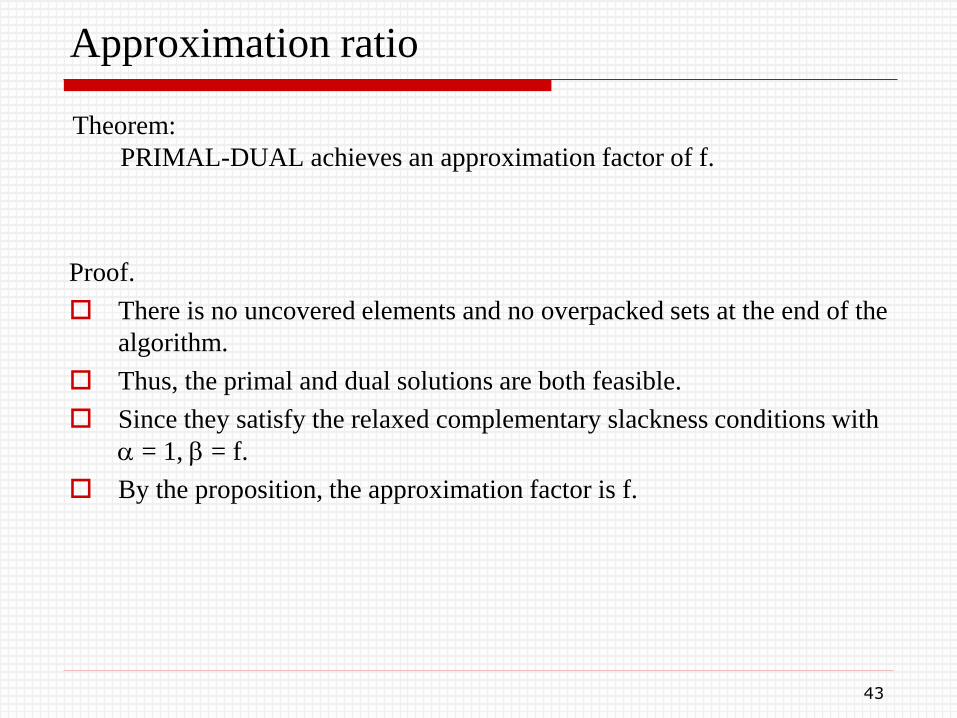
Approximation ratio
Theorem:
PRIMAL-DUAL achieves an approximation factor of f.
Proof.
There is no uncovered elements and no overpacked sets at the end of the
algorithm.
Thus, the primal and dual solutions are both feasible.
Since they satisfy the relaxed complementary slackness conditions with
= 1, = f.
By the proposition, the approximation factor is f.
43
Appeindix:Random Variables and TheirExpectations
Terminologies
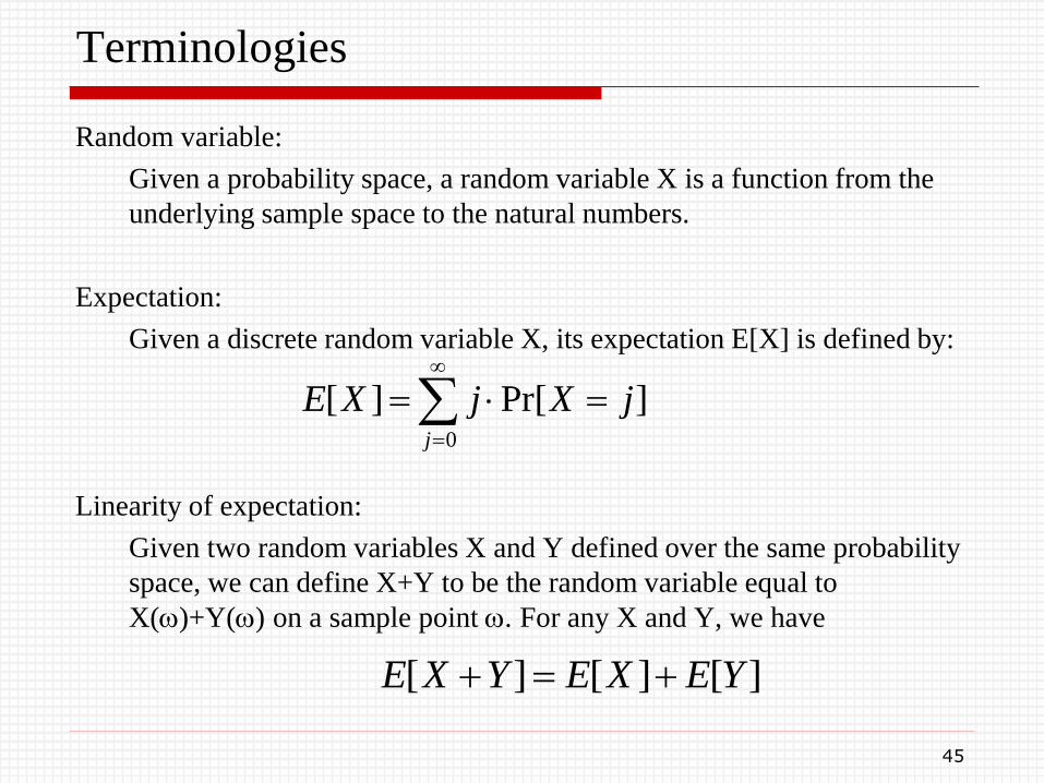
Random variable:
Given a probability space, a random variable X is a function from the
underlying sample space to the natural numbers.
Expectation:
Given a discrete random variable X, its expectation E[X] is defined by:
Linearity of expectation:
Given two random variables X and Y defined over the same probability
space, we can define X+Y to be the random variable equal to
X()+Y() on a sample point . For any X and Y, we have
45
0
]Pr[][j
jXjXE
][][][ YEXEYXE
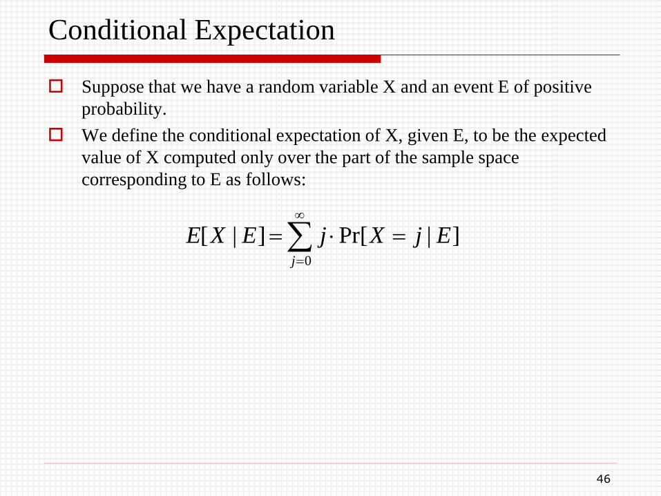
Conditional Expectation
Suppose that we have a random variable X and an event E of positive
probability.
We define the conditional expectation of X, given E, to be the expected
value of X computed only over the part of the sample space
corresponding to E as follows:
46
0
]|Pr[]|[j
EjXjEXE

Maximum Satisfiability
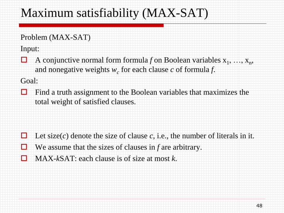
Maximum satisfiability (MAX-SAT)
Problem (MAX-SAT)
Input:
A conjunctive normal form formula f on Boolean variables x1, …, xn,
and nonegative weights wc for each clause c of formula f.
Goal:
Find a truth assignment to the Boolean variables that maximizes the
total weight of satisfied clauses.
Let size(c) denote the size of clause c, i.e., the number of literals in it.
We assume that the sizes of clauses in f are arbitrary.
MAX-kSAT: each clause is of size at most k.
48
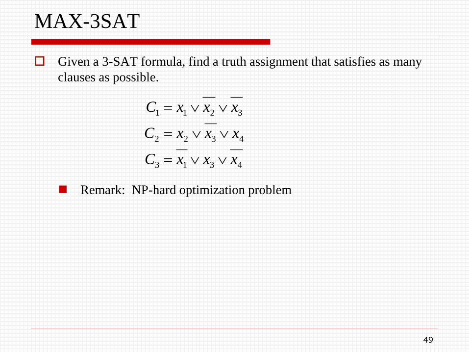
MAX-3SAT
Given a 3-SAT formula, find a truth assignment that satisfies as many
clauses as possible.
Remark: NP-hard optimization problem
49
4313
4322
3211
xxxC
xxxC
xxxC
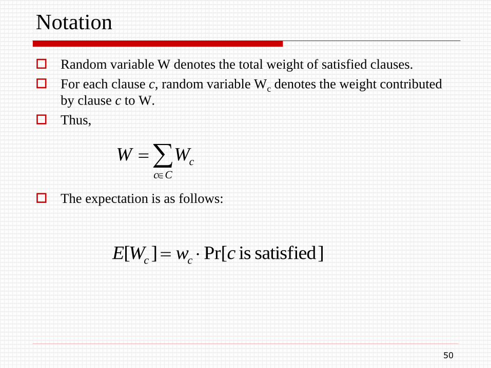
Notation
Random variable W denotes the total weight of satisfied clauses.
For each clause c, random variable Wc denotes the weight contributed
by clause c to W.
Thus,
The expectation is as follows:
50
Cc
cWW
]satisfied is Pr[][ cwWE cc
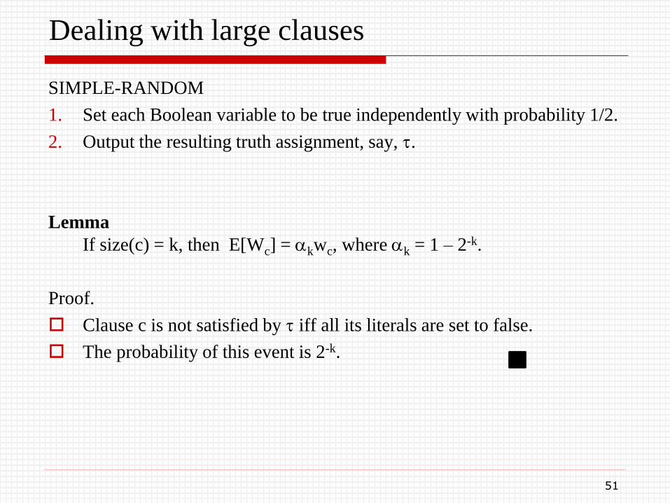
Dealing with large clauses
SIMPLE-RANDOM
1. Set each Boolean variable to be true independently with probability 1/2.
2. Output the resulting truth assignment, say, .
Lemma
If size(c) = k, then E[Wc] = kwc, where k = 1 – 2-k.
Proof.
Clause c is not satisfied by iff all its literals are set to false.
The probability of this event is 2-k.
51
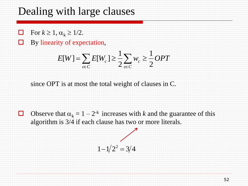
Dealing with large clauses
For k 1, k 1/2.
By linearity of expectation,
since OPT is at most the total weight of clauses in C.
Observe that k = 1 – 2-k increases with k and the guarantee of this
algorithm is 3/4 if each clause has two or more literals.
52
OPTwWEWECc
c
Cc
c2
1
2
1][][
43211 2
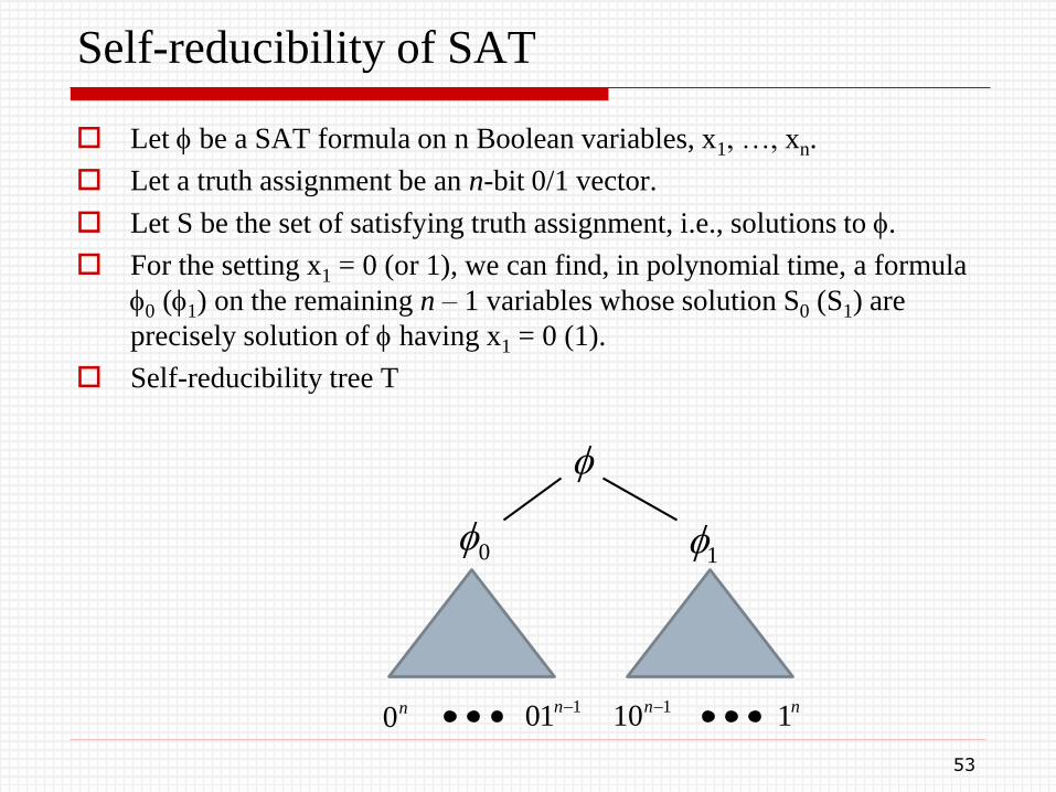
Self-reducibility of SAT
Let be a SAT formula on n Boolean variables, x1, …, xn.
Let a truth assignment be an n-bit 0/1 vector.
Let S be the set of satisfying truth assignment, i.e., solutions to .
For the setting x1 = 0 (or 1), we can find, in polynomial time, a formula
0 (1) on the remaining n – 1 variables whose solution S0 (S1) are
precisely solution of having x1 = 0 (1).
Self-reducibility tree T
53
0 1
n0110 n101 n n1
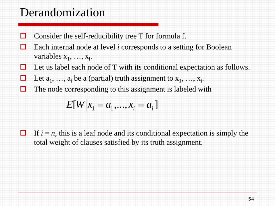
Derandomization
Consider the self-reducibility tree T for formula f.
Each internal node at level i corresponds to a setting for Boolean
variables x1, …, xi.
Let us label each node of T with its conditional expectation as follows.
Let a1, …, ai be a (partial) truth assignment to x1, …, xi.
The node corresponding to this assignment is labeled with
If i = n, this is a leaf node and its conditional expectation is simply the
total weight of clauses satisfied by its truth assignment.
54
],...,[ 11 ii axaxWE
Derandomizing via conditional expectation
Lemma
The conditional expectation of any node in T can be computed in
polynomial time.
Proof
Consider a node x1 = a1, …, xi = ai.
Let be the formula on variables xi+1, …, xn.
The expected weight of satisfied clauses of under a random truth
assignment to the variables xi+1, …, xn can be computed in polynomial
time.
Adding to this, the total weight of clauses of f already satisfied by the
partial assignment x1 = a1, …, xi = ai gives the answer.
55
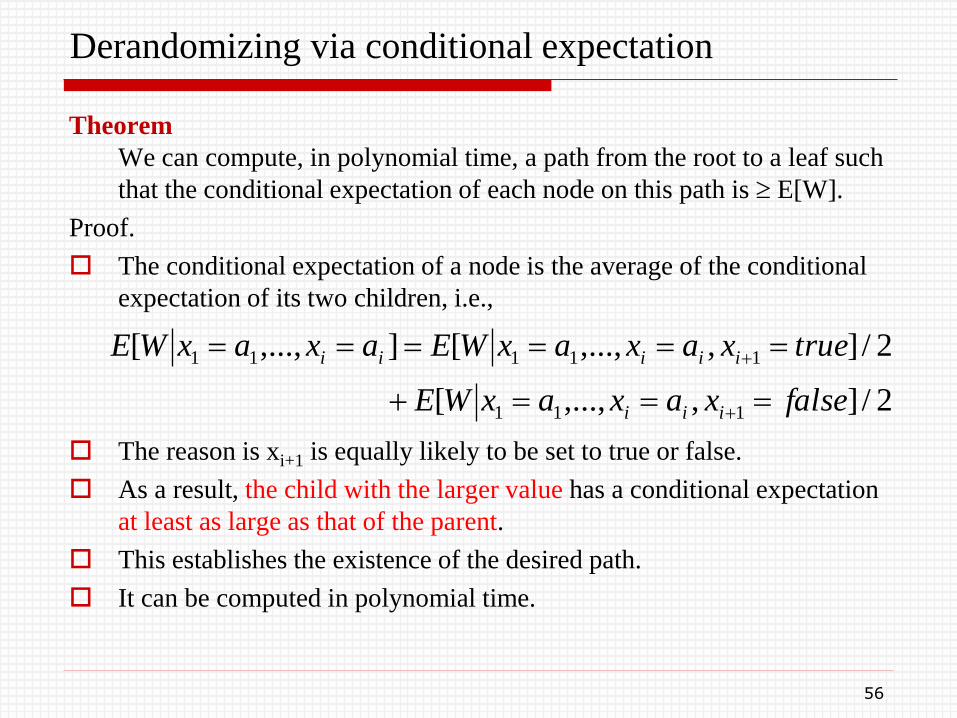
Derandomizing via conditional expectation
Theorem
We can compute, in polynomial time, a path from the root to a leaf such
that the conditional expectation of each node on this path is E[W].
Proof.
The conditional expectation of a node is the average of the conditional
expectation of its two children, i.e.,
The reason is xi+1 is equally likely to be set to true or false.
As a result, the child with the larger value has a conditional expectation
at least as large as that of the parent.
This establishes the existence of the desired path.
It can be computed in polynomial time.
56
2/],,...,[
2/],,...,[],...,[
111
11111
falsexaxaxWE
truexaxaxWEaxaxWE
iii
iiiii
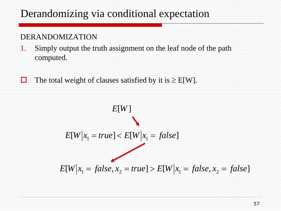
Derandomizing via conditional expectation
DERANDOMIZATION
1. Simply output the truth assignment on the leaf node of the path
computed.
The total weight of clauses satisfied by it is E[W].
57
][WE
][][ 11 falsexWEtruexWE
],[],[ 2121 falsexfalsexWEtruexfalsexWE
General method
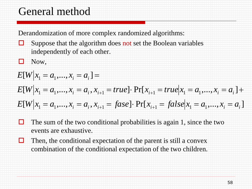
Derandomization of more complex randomized algorithms:
Suppose that the algorithm does not set the Boolean variables
independently of each other.
Now,
The sum of the two conditional probabilities is again 1, since the two
events are exhaustive.
Then, the conditional expectation of the parent is still a convex
combination of the conditional expectation of the two children.
58
],...,Pr[],,...,[
],...,Pr[],,...,[
],...,[
111111
111111
11
iiiiii
iiiiii
ii
axaxfalsexfasexaxaxWE
axaxtruextruexaxaxWE
axaxWE
General method
If we can determine, in polynomial time, which of the two children has
a larger value, we can again derandomize the algorithm.
(However, computing the conditional expectations may not be easy.)
In general, a randomized algorithm may pick from a larger set of
choices and not necessarily with equal probability.
But, given by the probabilities of picking them, a convex combination
of the conditional expectations of these choices equals the conditional
expectation of the parent.
Hence, there must be a choice that has at least as large as a conditional
expectation as the parent.
59
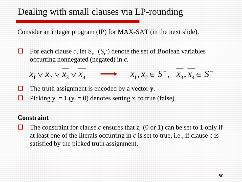
Dealing with small clauses via LP-rounding
Consider an integer program (IP) for MAX-SAT (in the next slide).
For each clause c, let Sc+ (Sc
-) denote the set of Boolean variables
occurring nonnegated (negated) in c.
The truth assignment is encoded by a vector y.
Picking yi = 1 (yi = 0) denotes setting xi to true (false).
Constraint
The constraint for clause c ensures that zc (0 or 1) can be set to 1 only if
at least one of the literals occurring in c is set to true, i.e., if clause c is
satisfied by the picked truth assignment.
60
4321 xxxx SxxSxx 4321 ,,,
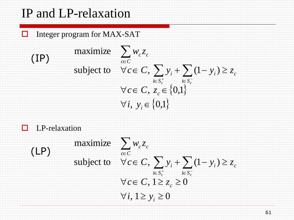
IP and LP-relaxation
Integer program for MAX-SAT
LP-relaxation
61
1,0,
1,0,
)1(,subject to
maximize
i
c
c
Si
i
Si
i
Cc
cc
yi
zCc
zyyCc
zw
cc
01,
01,
)1(,subject to
maximize
i
c
c
Si
i
Si
i
Cc
cc
yi
zCc
zyyCc
zw
cc
(IP)
(LP)
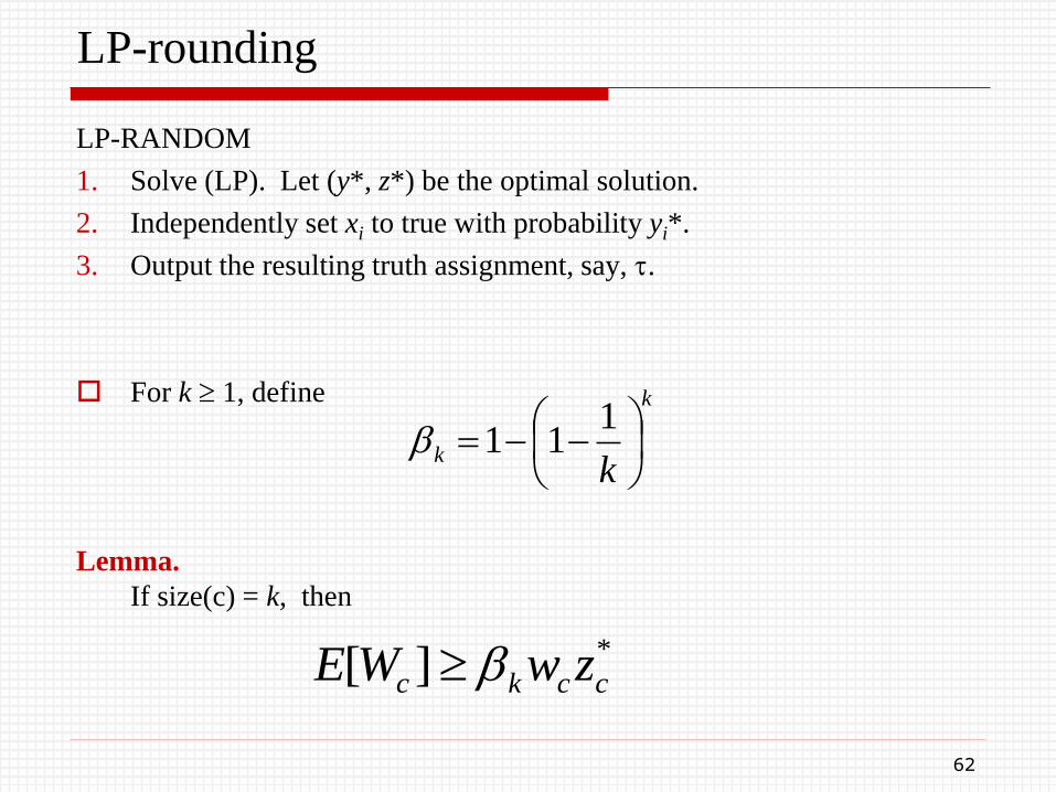
LP-rounding
LP-RANDOM
1. Solve (LP). Let (y*, z*) be the optimal solution.
2. Independently set xi to true with probability yi*.
3. Output the resulting truth assignment, say, .
For k 1, define
Lemma.
If size(c) = k, then
62
k
kk
111
*][ cckc zwWE
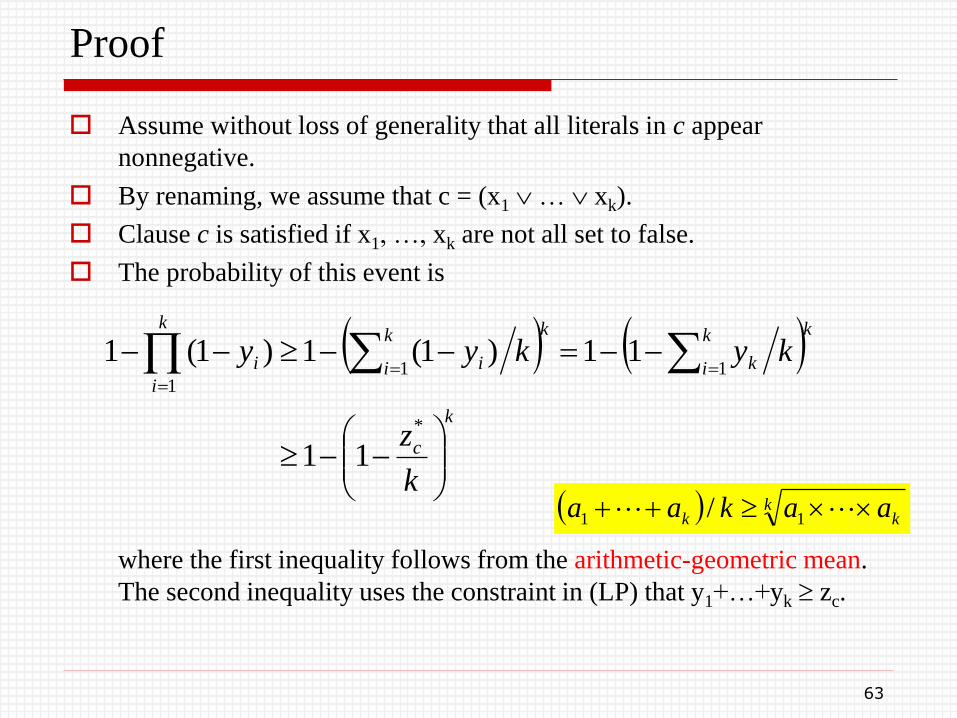
Proof
Assume without loss of generality that all literals in c appear
nonnegative.
By renaming, we assume that c = (x1 … xk).
Clause c is satisfied if x1, …, xk are not all set to false.
The probability of this event is
where the first inequality follows from the arithmetic-geometric mean.
The second inequality uses the constraint in (LP) that y1+…+yk zc.
63
k
c
kk
i k
kk
i i
k
i
i
k
z
kykyy
*
111
11
11)1(1)1(1
kkk aakaa 11 /
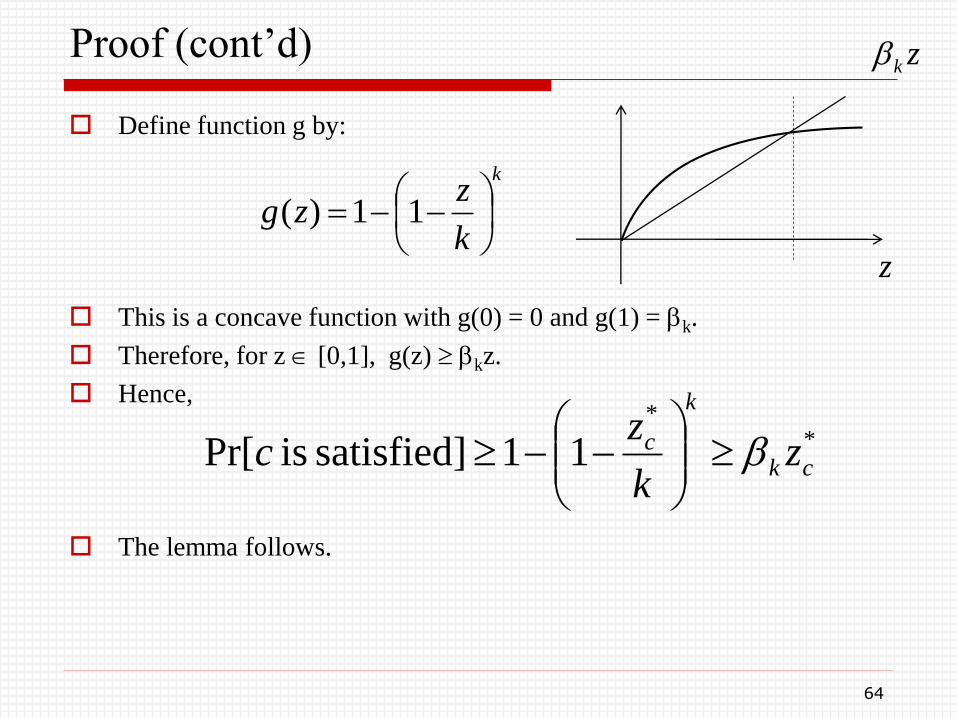
Proof (cont’d)
Define function g by:
This is a concave function with g(0) = 0 and g(1) = k.
Therefore, for z [0,1], g(z) kz.
Hence,
The lemma follows.
64
k
k
zzg
11)(
**
11]satisfied is Pr[ ck
k
c zk
zc
zk
z
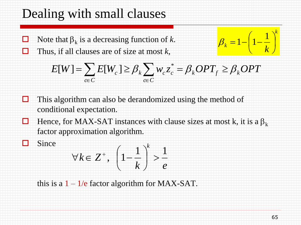
Dealing with small clauses
Note that k is a decreasing function of k.
Thus, if all clauses are of size at most k,
This algorithm can also be derandomized using the method of
conditional expectation.
Hence, for MAX-SAT instances with clause sizes at most k, it is a k
factor approximation algorithm.
Since
this is a 1 – 1/e factor algorithm for MAX-SAT.
65
OPTOPTzwWEWE kfk
Cc
cck
Cc
c
*][][
ekZk
k11
1,
k
kk
111
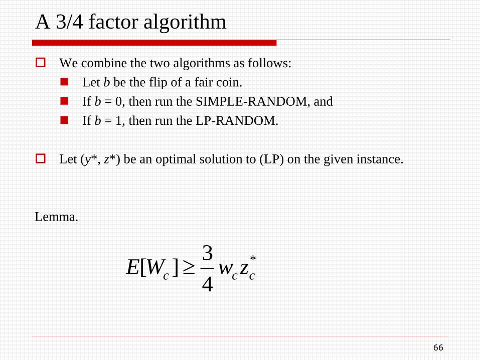
A 3/4 factor algorithm
We combine the two algorithms as follows:
Let b be the flip of a fair coin.
If b = 0, then run the SIMPLE-RANDOM, and
If b = 1, then run the LP-RANDOM.
Let (y*, z*) be an optimal solution to (LP) on the given instance.
Lemma.
66
*
4
3][ ccc zwWE
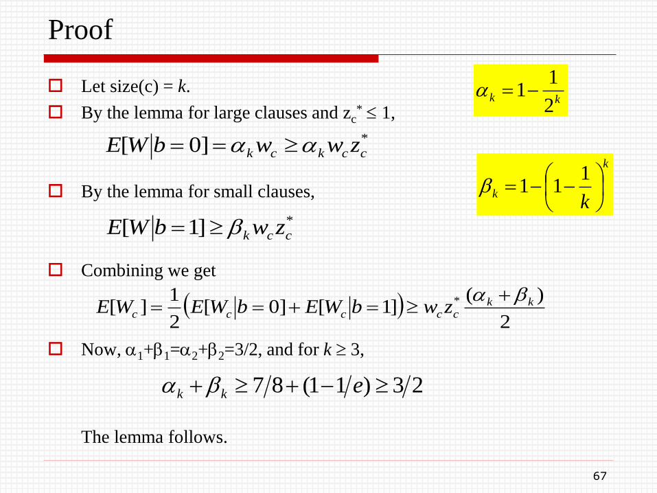
Proof
Let size(c) = k.
By the lemma for large clauses and zc* 1,
By the lemma for small clauses,
Combining we get
Now, 1+1=2+2=3/2, and for k 3,
The lemma follows.
67
*]0[ cckck zwwbWE
*]1[ cck zwbWE
2
)(]1[]0[
2
1][ * kk
ccccc zwbWEbWEWE
23)11(87 ekk
kk2
11
k
kk
111
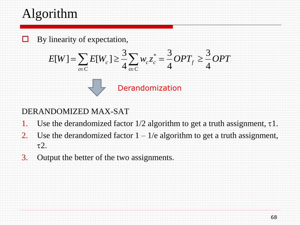
Algorithm
By linearity of expectation,
DERANDOMIZED MAX-SAT
1. Use the derandomized factor 1/2 algorithm to get a truth assignment, 1.
2. Use the derandomized factor 1 – 1/e algorithm to get a truth assignment,
2.
3. Output the better of the two assignments.
68
OPTOPTzwWEWE f
Cc
cc
Cc
c4
3
4
3
4
3][][ *
Derandomization
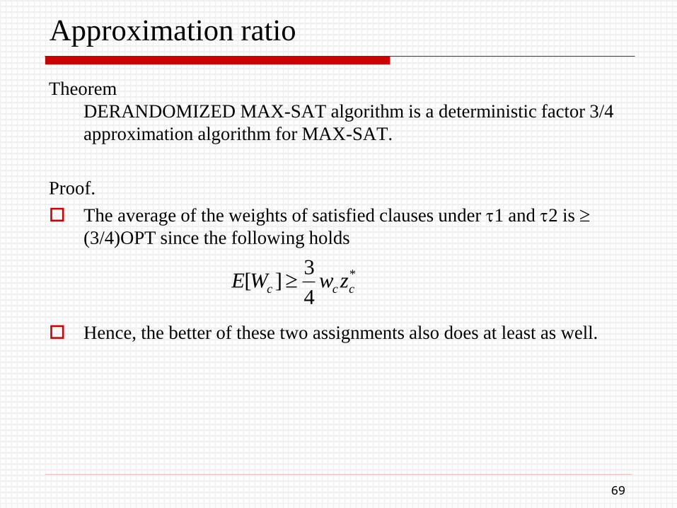
Approximation ratio
Theorem
DERANDOMIZED MAX-SAT algorithm is a deterministic factor 3/4
approximation algorithm for MAX-SAT.
Proof.
The average of the weights of satisfied clauses under 1 and 2 is
(3/4)OPT since the following holds
Hence, the better of these two assignments also does at least as well.
69
*
4
3][ ccc zwWE
Semidefinite Programming (SDP)
Outline
We provide a class of relaxations, called vector programs.
These serve as relaxation for several NP-hard problems, in particular,
for problems that can be expressed as strict quadratic programs.
Vector programs are equivalent to a powerful and well-studied
generalization of linear programs, called semidefinite programs.
Semidefinite programs (and vector programs) can be solved within an
additive error of , for any >0, in time polynomial in n and log(1/),
using the ellipsoid algorithm.
We see the use of vector programs by deriving a 0.87856 factor
approximation algorithm for MAX-CUT.
71
Maximum cut
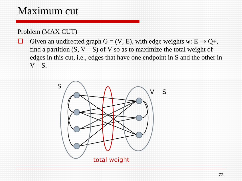
Problem (MAX CUT)
Given an undirected graph G = (V, E), with edge weights w: E Q+,
find a partition (S, V – S) of V so as to maximize the total weight of
edges in this cut, i.e., edges that have one endpoint in S and the other in
V – S.
72
SV – S
total weight
Strict quadratic programs
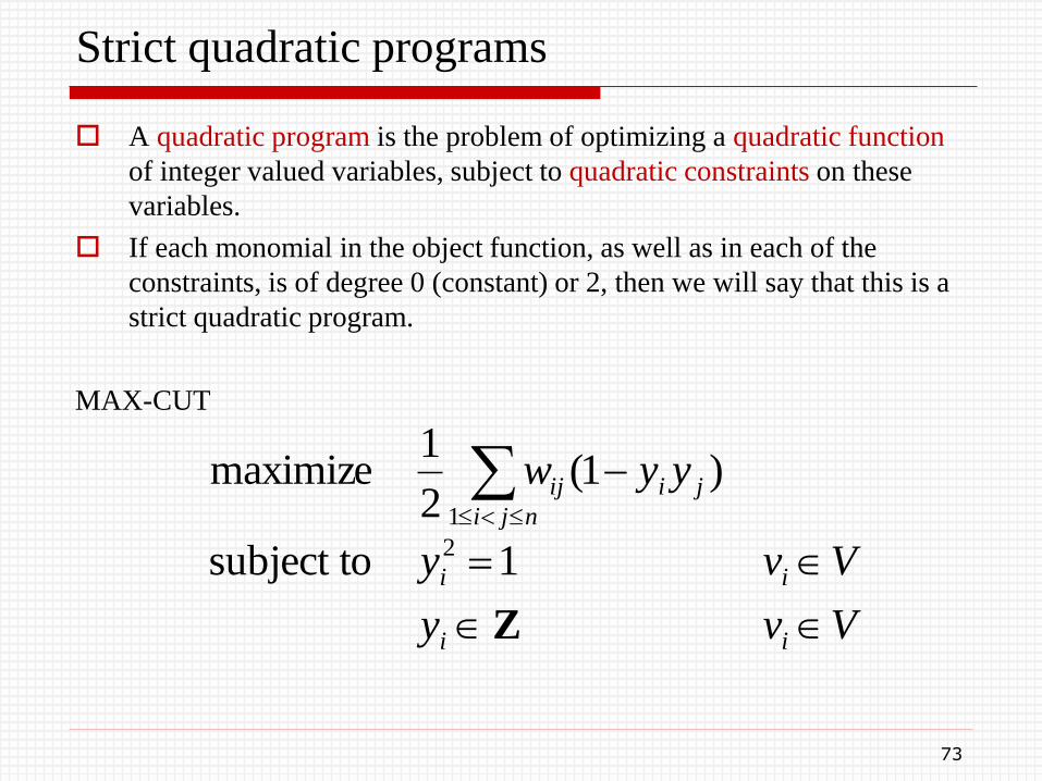
A quadratic program is the problem of optimizing a quadratic function
of integer valued variables, subject to quadratic constraints on these
variables.
If each monomial in the object function, as well as in each of the
constraints, is of degree 0 (constant) or 2, then we will say that this is a
strict quadratic program.
MAX-CUT
Vvy
Vvy
yyw
ii
ii
nji
jiij
Z
1subject to
)1(2
1maximize
2
1
73
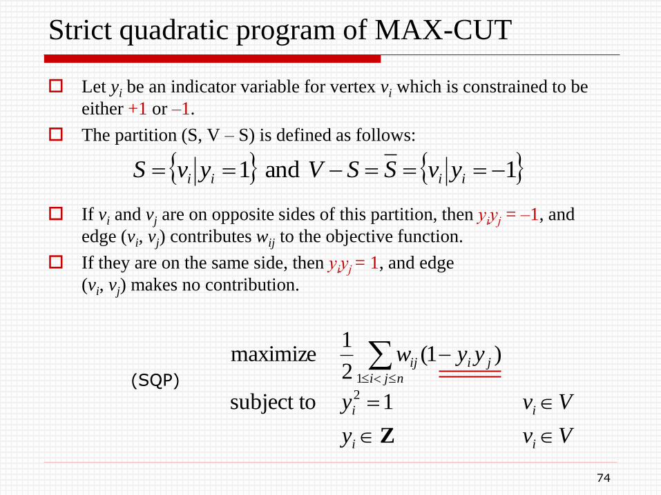
Strict quadratic program of MAX-CUT
Let yi be an indicator variable for vertex vi which is constrained to be
either +1 or –1.
The partition (S, V – S) is defined as follows:
If vi and vj are on opposite sides of this partition, then yiyj = –1, and
edge (vi, vj) contributes wij to the objective function.
If they are on the same side, then yiyj = 1, and edge
(vi, vj) makes no contribution.
1 and 1 iiii yvSSVyvS
Vvy
Vvy
yyw
ii
ii
nji
jiij
Z
1subject to
)1(2
1maximize
2
1(SQP)
74
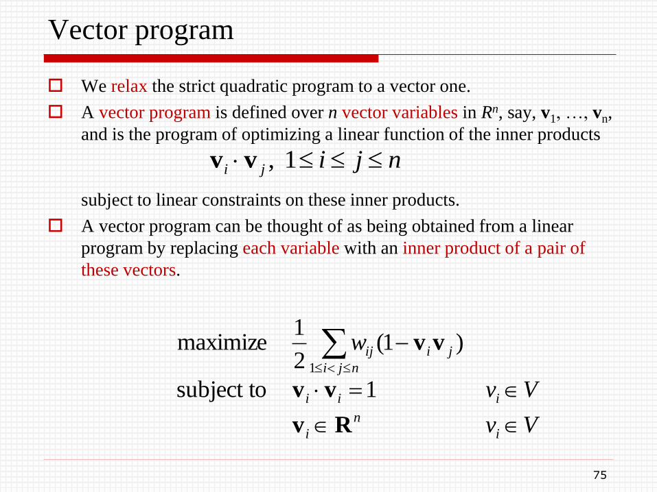
Vector program
We relax the strict quadratic program to a vector one.
A vector program is defined over n vector variables in Rn, say, v1, …, vn,
and is the program of optimizing a linear function of the inner products
subject to linear constraints on these inner products.
A vector program can be thought of as being obtained from a linear
program by replacing each variable with an inner product of a pair of
these vectors.
njiji 1,vv
Vv
Vv
w
i
n
i
iii
nji
jiij
Rv
vv
vv
1subject to
)1(2
1maximize
1
75
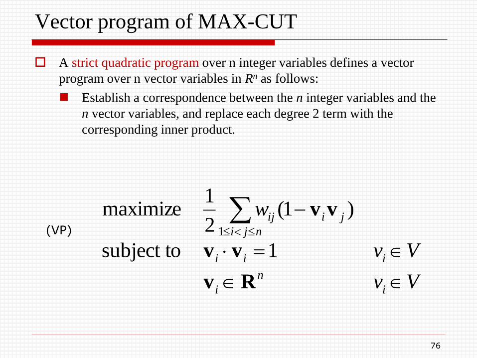
Vector program of MAX-CUT
A strict quadratic program over n integer variables defines a vector
program over n vector variables in Rn as follows:
Establish a correspondence between the n integer variables and the
n vector variables, and replace each degree 2 term with the
corresponding inner product.
Vv
Vv
w
i
n
i
iii
nji
jiij
Rv
vv
vv
1subject to
)1(2
1maximize
1(VP)
76
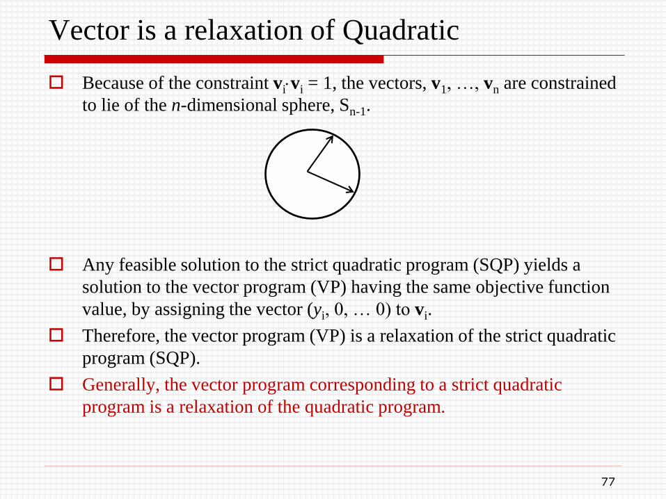
Vector is a relaxation of Quadratic
Because of the constraint vivi = 1, the vectors, v1, …, vn are constrained
to lie of the n-dimensional sphere, Sn-1.
Any feasible solution to the strict quadratic program (SQP) yields a
solution to the vector program (VP) having the same objective function
value, by assigning the vector (yi, 0, … 0) to vi.
Therefore, the vector program (VP) is a relaxation of the strict quadratic
program (SQP).
Generally, the vector program corresponding to a strict quadratic
program is a relaxation of the quadratic program.
77
Approximability of vector programs
Vector programs are approximable to any desired degree of accuracy in
polynomial time, and thus the relaxation (VP) provides an upper bound
on OPT for MAX-CUT.
To show the above, we need to recall some interesting and powerful
properties of positive semidefinite matrices.
78
Properties of positive semidefinite matrices
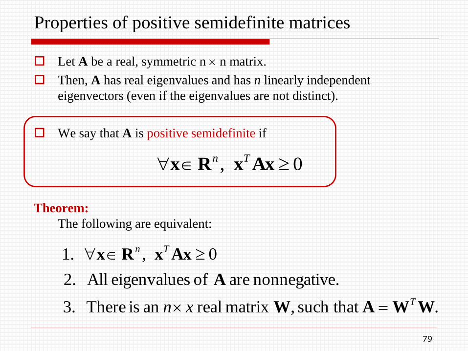
Let A be a real, symmetric n n matrix.
Then, A has real eigenvalues and has n linearly independent
eigenvectors (even if the eigenvalues are not distinct).
We say that A is positive semidefinite if
Theorem:
The following are equivalent:
0, AxxRx Tn
.such that ,matrix real an is There.3
e.nonnegativ are of seigenvalue All.2
0,.1
WWAW
A
AxxRx
T
Tn
xn
79
Proof
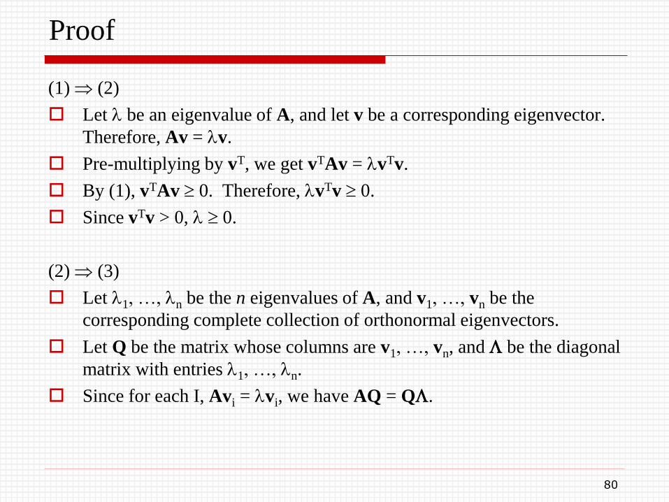
(1) (2)
Let be an eigenvalue of A, and let v be a corresponding eigenvector.
Therefore, Av = v.
Pre-multiplying by vT, we get vTAv = vTv.
By (1), vTAv 0. Therefore, vTv 0.
Since vTv > 0, 0.
(2) (3)
Let 1, …, n be the n eigenvalues of A, and v1, …, vn be the
corresponding complete collection of orthonormal eigenvectors.
Let Q be the matrix whose columns are v1, …, vn, and be the diagonal
matrix with entries 1, …, n.
Since for each I, Avi = vi, we have AQ = Q.
80
Proof (cont’d)
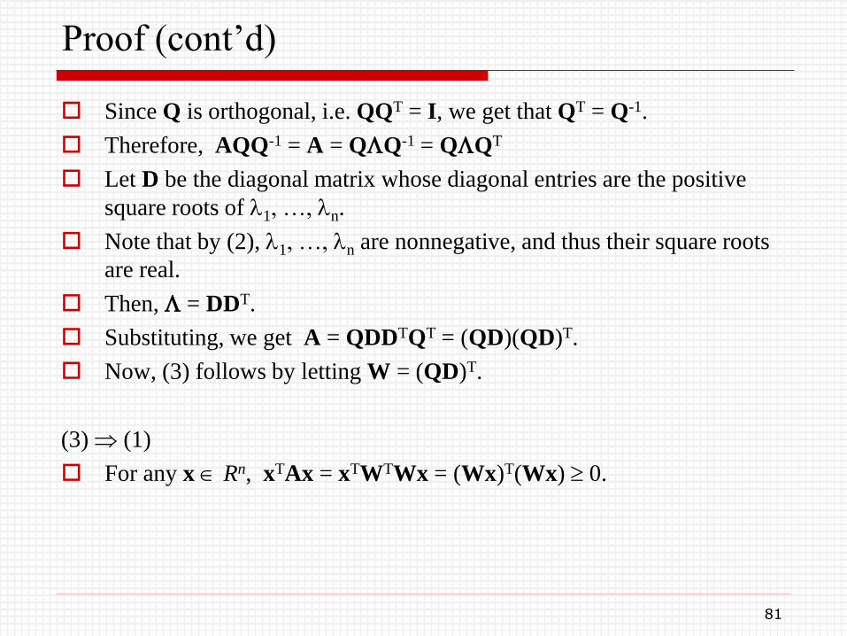
Since Q is orthogonal, i.e. QQT = I, we get that QT = Q-1.
Therefore, AQQ-1 = A = QQ-1 = QQT
Let D be the diagonal matrix whose diagonal entries are the positive
square roots of 1, …, n.
Note that by (2), 1, …, n are nonnegative, and thus their square roots
are real.
Then, = DDT.
Substituting, we get A = QDDTQT = (QD)(QD)T.
Now, (3) follows by letting W = (QD)T.
(3) (1)
For any x Rn, xTAx = xTWTWx = (Wx)T(Wx) 0.
81
Semidefinite programming problem
Let Y be an n n matrix of real variables.
The problem of maximizing a linear function of yij’s, subject to linear
constraints on them, and the additional constraint that Y be symmetric
and positive semidefinite, is called the semidefinite programming
problem (SDP).
82
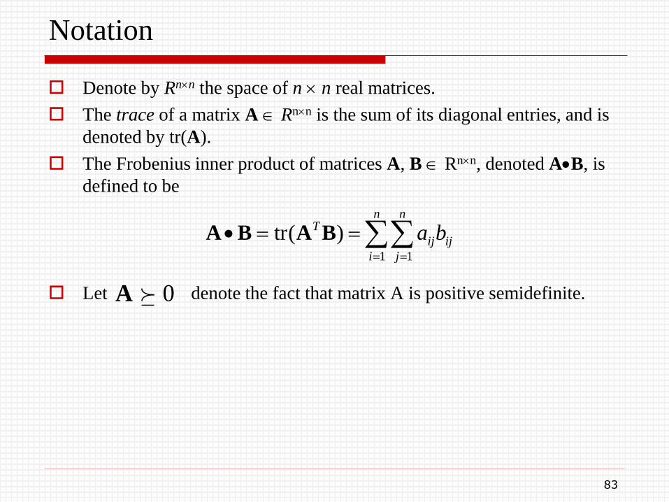
Notation
Denote by Rnn the space of n n real matrices.
The trace of a matrix A Rnn is the sum of its diagonal entries, and is
denoted by tr(A).
The Frobenius inner product of matrices A, B Rnn, denoted AB, is
defined to be
Let denote the fact that matrix A is positive semidefinite.
n
i
n
j
ijij
T ba1 1
)(tr BABA
0A
83
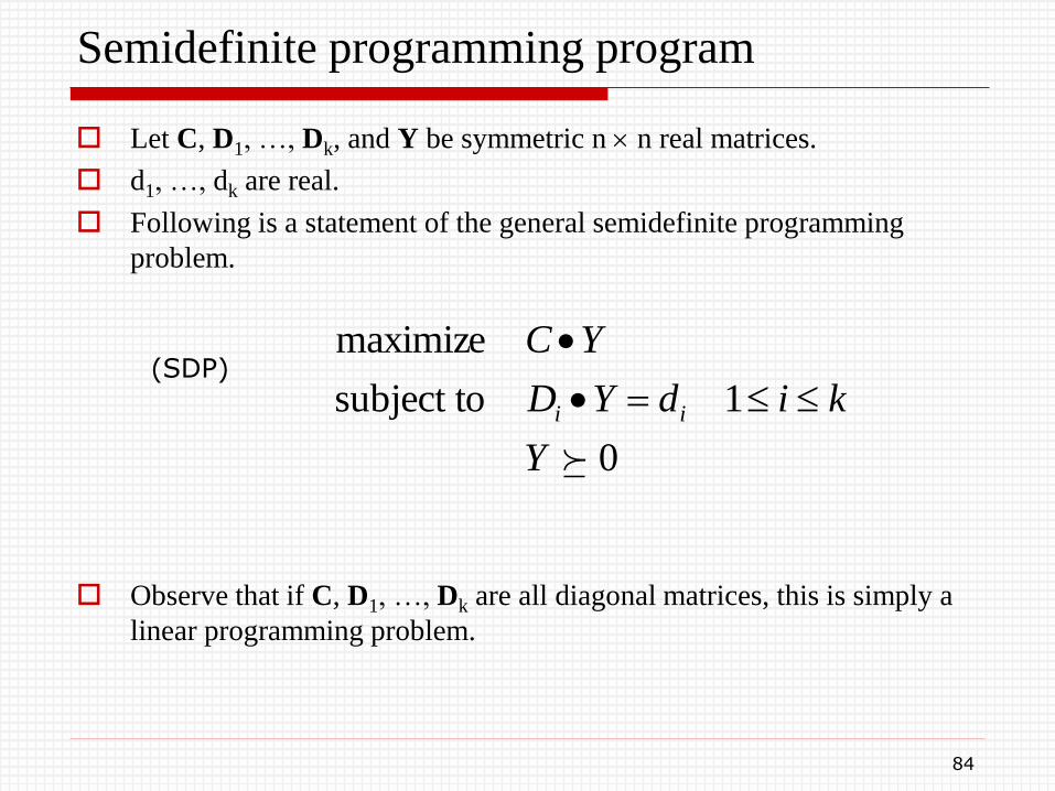
Semidefinite programming program
Let C, D1, …, Dk, and Y be symmetric n n real matrices.
d1, …, dk are real.
Following is a statement of the general semidefinite programming
problem.
Observe that if C, D1, …, Dk are all diagonal matrices, this is simply a
linear programming problem.
0
1subject to
maximize
Y
kidYD
YC
ii
(SDP)
84
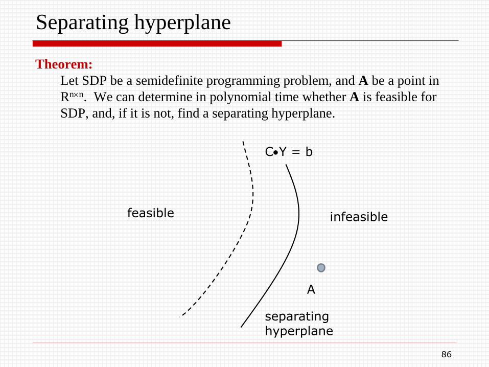
Separating hyperplane
Let us call a matrix satisfying all the constraints of (SDP) a feasible
solution.
Since a convex combination of positive semidefinite matrices is positive
semidefinite, it is easy to see that the set of feasible solutions is convex.
I.e., if A and B are feasible solutions, then so is any convex
combination of these solutions.
Let A be an infeasible point.
A hyperplane CY b is called a separating hyperplane for A if all
feasible points satisfy it and point A does not satisfy it.
In the next slide, we show how to find a separating hyperplane in
polynomial time.
As a consequence, for any > 0, semidefinite programs can be solved
within an additive error of , in time polynomial in n and log(1/), using
the ellipsoid algorithm.
85
Separating hyperplane
Theorem:
Let SDP be a semidefinite programming problem, and A be a point in
Rnn. We can determine in polynomial time whether A is feasible for
SDP, and, if it is not, find a separating hyperplane.
feasible infeasible
A
CY = b
separatinghyperplane
86
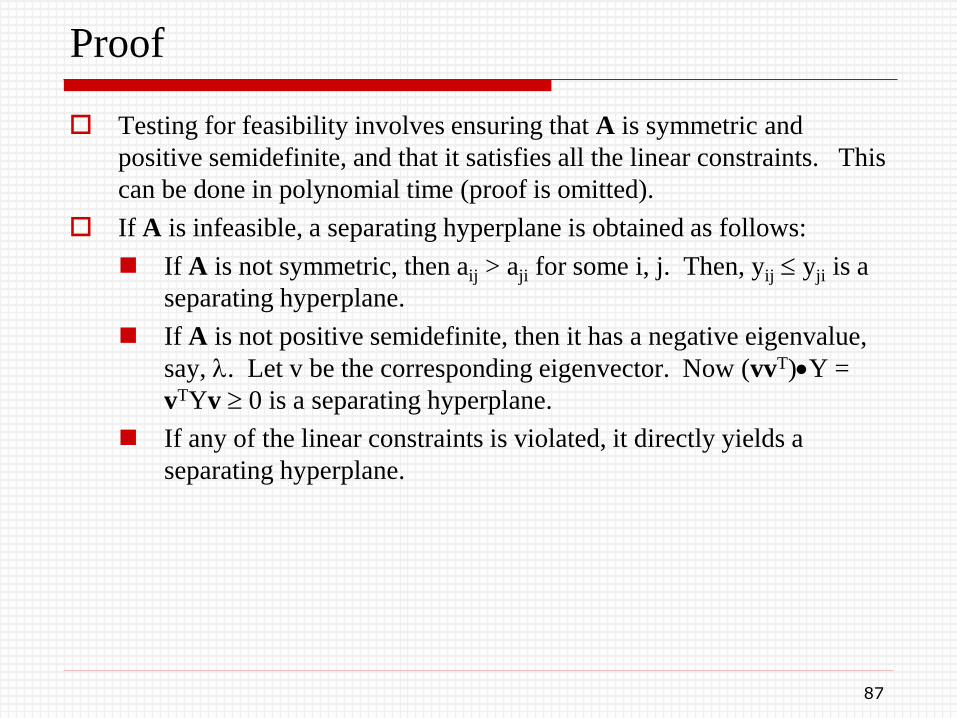
Proof
Testing for feasibility involves ensuring that A is symmetric and
positive semidefinite, and that it satisfies all the linear constraints. This
can be done in polynomial time (proof is omitted).
If A is infeasible, a separating hyperplane is obtained as follows:
If A is not symmetric, then aij > aji for some i, j. Then, yij yji is a
separating hyperplane.
If A is not positive semidefinite, then it has a negative eigenvalue,
say, . Let v be the corresponding eigenvector. Now (vvT)Y =
vTYv 0 is a separating hyperplane.
If any of the linear constraints is violated, it directly yields a
separating hyperplane.
87
Equivalency
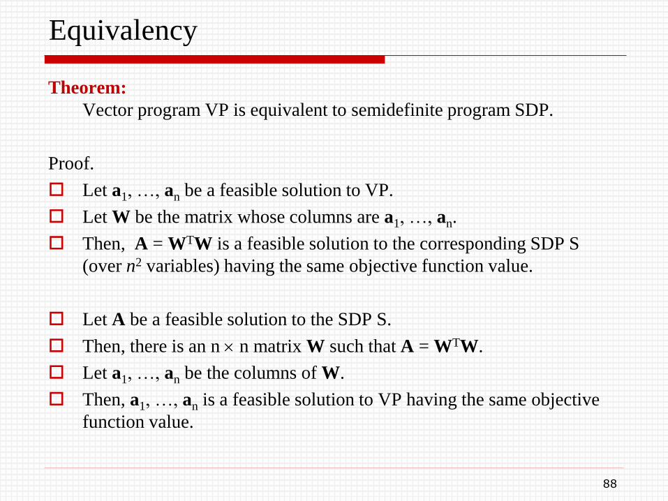
Theorem:
Vector program VP is equivalent to semidefinite program SDP.
Proof.
Let a1, …, an be a feasible solution to VP.
Let W be the matrix whose columns are a1, …, an.
Then, A = WTW is a feasible solution to the corresponding SDP S
(over n2 variables) having the same objective function value.
Let A be a feasible solution to the SDP S.
Then, there is an n n matrix W such that A = WTW.
Let a1, …, an be the columns of W.
Then, a1, …, an is a feasible solution to VP having the same objective
function value.
88
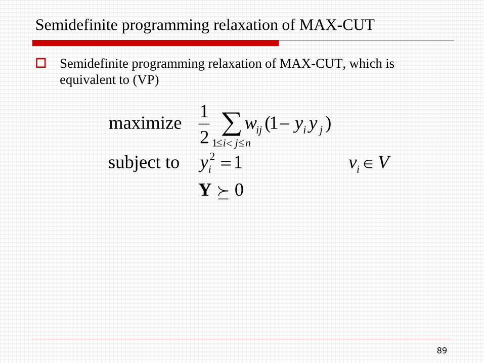
Semidefinite programming relaxation of MAX-CUT
Semidefinite programming relaxation of MAX-CUT, which is
equivalent to (VP)
0
1subject to
)1(2
1maximize
2
1
Y
Vvy
yyw
ii
nji
jiij
89
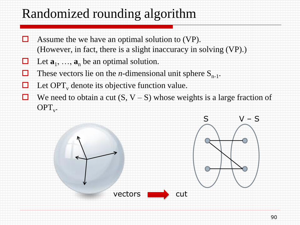
Randomized rounding algorithm
Assume the we have an optimal solution to (VP).
(However, in fact, there is a slight inaccuracy in solving (VP).)
Let a1, …, an be an optimal solution.
These vectors lie on the n-dimensional unit sphere Sn-1.
Let OPTv denote its objective function value.
We need to obtain a cut (S, V – S) whose weights is a large fraction of
OPTv.
90
S V – S
vectors cut
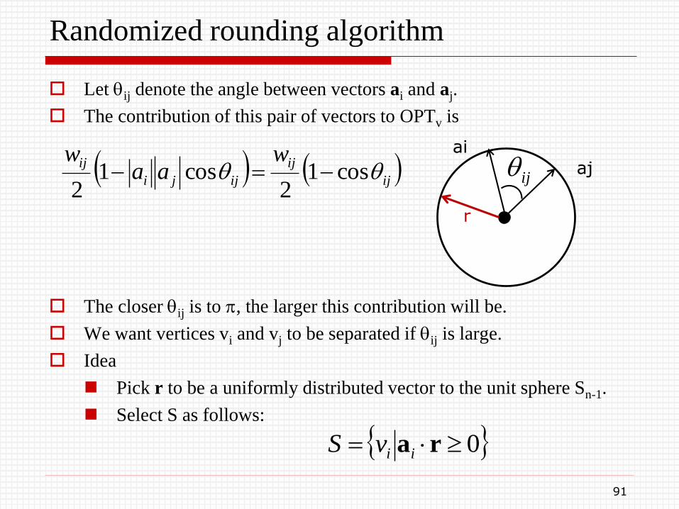
Randomized rounding algorithm
Let ij denote the angle between vectors ai and aj.
The contribution of this pair of vectors to OPTv is
The closer ij is to , the larger this contribution will be.
We want vertices vi and vj to be separated if ij is large.
Idea
Pick r to be a uniformly distributed vector to the unit sphere Sn-1.
Select S as follows:
91
ai
ajij ij
ij
ijji
ij waa
w cos1
2cos1
2
0 raiivS
r
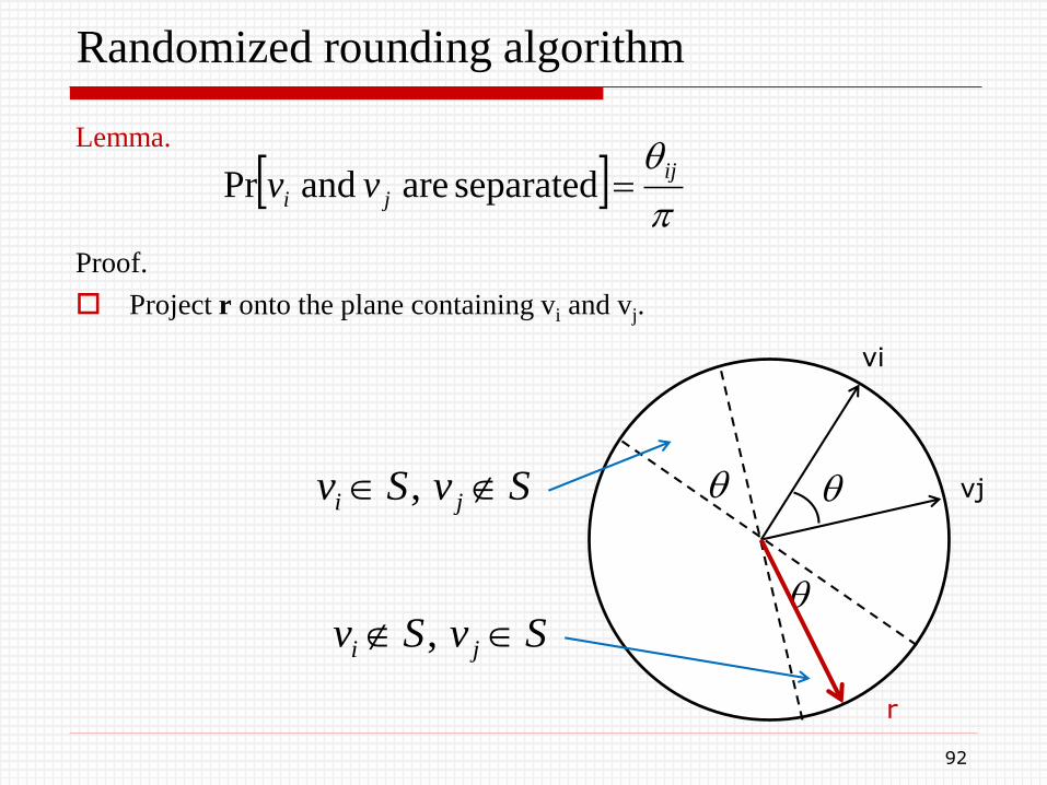
Randomized rounding algorithm
Lemma.
Proof.
Project r onto the plane containing vi and vj.
92
ij
ji vv separated are and Pr
vi
vj
SvSv ji ,
SvSv ji ,
r
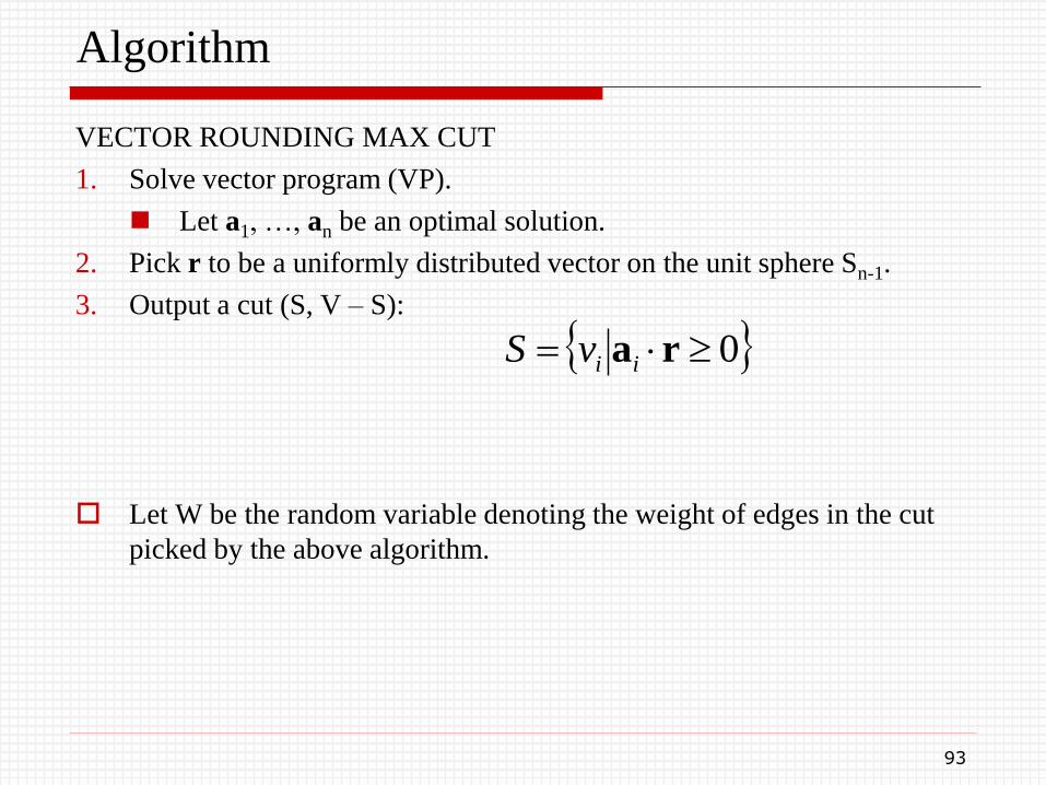
Algorithm
VECTOR ROUNDING MAX CUT
1. Solve vector program (VP).
Let a1, …, an be an optimal solution.
2. Pick r to be a uniformly distributed vector on the unit sphere Sn-1.
3. Output a cut (S, V – S):
Let W be the random variable denoting the weight of edges in the cut
picked by the above algorithm.
93
0 raiivS
Approximation ratio
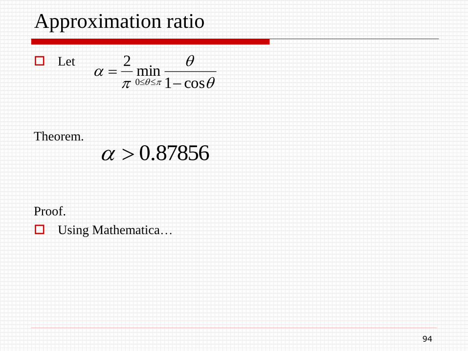
Let
Theorem.
Proof.
Using Mathematica…
94
cos1min
2
0
87856.0
Approximation ratio
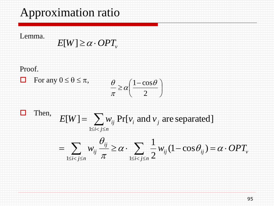
Lemma.
Proof.
For any 0 ,
Then,
95
vOPTWE ][
2
cos1
v
nji
ijij
nji
ij
ij
nji
jiij
OPTww
vvwWE
11
1
)cos1(2
1
]separated are and Pr[][
Approximation ratio
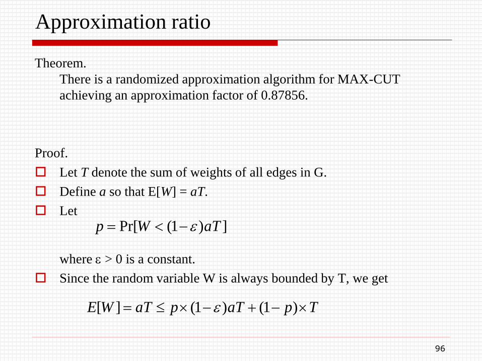
Theorem.
There is a randomized approximation algorithm for MAX-CUT
achieving an approximation factor of 0.87856.
Proof.
Let T denote the sum of weights of all edges in G.
Define a so that E[W] = aT.
Let
where > 0 is a constant.
Since the random variable W is always bounded by T, we get
96
])1(Pr[ aTWp
TpaTpaTWE )1()1(][

Proof (cont’d)
Therefore,
Now,
where the last inequality follows from the fact that OPT T/2.
Therefore,
Using this upper and lower bound on a, we get
97
aa
ap
1
1
2][
TOPTOPTaTWET v
21
a
.2/1
2/where,1
2/1
2/1
ccp
Proof (cont’d)
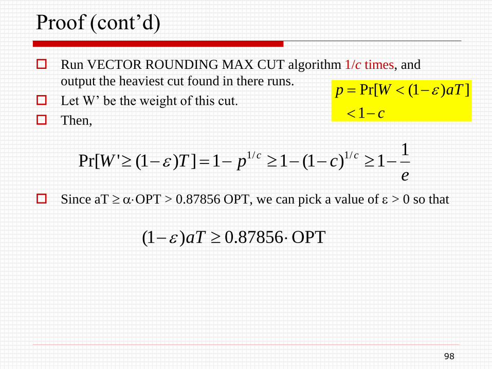
Run VECTOR ROUNDING MAX CUT algorithm 1/c times, and
output the heaviest cut found in there runs.
Let W’ be the weight of this cut.
Then,
Since aT OPT > 0.87856 OPT, we can pick a value of > 0 so that
98
ecpTW cc 1
1)1(11])1('Pr[ /1/1
c
aTWp
1
])1(Pr[
OPT87856.0)1( aT