arti–cial states - weatherhead center for international …€“cial states alberto alesina,...

Arti�cial States�

Alberto Alesina, William Easterly and Janina MatuszeskiHarvard University, New York University and Harvard University

February 2006Revised: May 2006

Abstract

Arti�cial states are those in which political borders do not coincidewith a division of nationalities desired by the people on the ground. Wepropose and compute for all countries in the world two new measures howarti�cial states are. One is based on measuring how borders split ethnicgroups into two separate adjacent countries. The other one measures howstraight land borders are, under the assumption the straight land bordersare more likely to be arti�cial. We then show that these two measures seemto be highly correlated with several measures of political and economicsuccess.

1 Introduction

Arti�cial states are those in which political borders do not coincide with a divi-sion of nationalities desired by the people on the ground. Former colonizers orpost war agreement amongst winners regarding borders have often created mon-strosities in which ethnic or religious or linguistic groups were thrown togetheror separated without any respect for peoples�aspirations. Eighty per cent ofAfrican borders follow latitudinal and longitudinal lines and many scholars be-lieve that such arti�cial (unnatural) borders which create ethnically fragmentedcountries or, conversely, separate into bordering countries the same people, areat the roots of Africa�s economic tragedy.1 Not only in Africa but everywhere

�We thank Jean Marie Baland, Alberto Bravo-Biosca, Ernesto dal Bo, Ashley Lester, andparticipants at conferences at Brown, NBER and a seminar at Harvard for useful comments.For much needed help with maps we thank Patrick Florance, Kimberly Karish and MichaelOltmans. Alesina gratefully acknowledges �nancial support from the NSF with a grant troughNBER.

1See Easterly and Levine (1997) for early econometric work on this point. Herbs (2000) andespecially Englebert Tarango and Carter (2002) focus on the arbitrariness of African bordersas an explanation of politico economic failures in this region. At the time of decolonization,new rulers in Africa made the decision to keep the borders drawn by former colonizers to avoiddisruptive con�icts amongst themselves.

2

around the globe from Iraq to the Middle East failed states, con�ict and eco-nomic misery often are very visible around borders left over by former colonizers,borders that had little resemblance to natural division of peoples.

There are three ways in which those who drew borders created problems.First they gave territories to one group ignoring the fact that another group hadalready claimed the same territory. Second, they drew boundaries lines splittingethnic (or religious or linguistic) groups into di¤erent countries, frustrating na-tional ambitions of various groups and creating unrest in the countries formed.Third they combined into a single country groups that wanted independence.The results can be disastrous. Arti�cial borders increase the motivation to safe-guard or advance nationalist agendas at the expense of economic and politicaldevelopment. As George Bernard Shaw eloquently put it "A healthy nation isas unconscious of its nationality as a healthy man is unconscious of his health.But if you break a nation�s nationality it will think of nothing else but gettingis set again."While the nature of borders has been mentioned in the political science (es-

pecially) and economic literature, we are not aware of systematic work relatingthe nature of country borders to the economic success of countries. Our goal isto provide measures that proxy for how natural or arti�cial of borders and relatethem to economic and political development. By arti�cial we mean a politicalborder drawn by individuals not living in the areas divided by these borders,normally former colonizers. All the other borders call them natural, are drawnby people on the ground. Needless to say often borders start as arti�cial andthen get modi�ed by people on the ground. Not only, but adjustments on theground may or may not re�ect the desire of a majority of the people living thereespecially if dictatorial regimes make such adjustments.We provide two measures never before used in econometric analysis of com-

parative development. One is relatively simple and captures whether or not anethnic group is "cut" by a political border line. That is, we measure situationsin which the same ethnic group is present in two bordering countries. Thismeasure accounts fairly precisely for one of the ways in which borders may be"wrong", that is when they cut through groups left in separate countries. Butit does not capture other ways in which borders may be undesirable; for in-stance situations in which two ethnic groups are forced into the same country.We then provide a second measure, based upon the assumption that if a landborder is close to a straight line it is more likely to be drawn arti�cially i.e. byformer colonizers; if it is relatively squiggly it is more likely to represent eithergeographic features (rivers, mountains etc.) and/or represent divisions carvedout in time to separate di¤erent people. This second measure probably comecloser to capturing instances in which lines drawn at former colonizers�tableshave stuck to the ground. The �rst measure may also capture adjustments ofborders on the ground that do not re�ect an appropriate division of people onthe ground. Needless to say the measure is not perfect but much of our paperis about precisely discussing this measure and alternatives. It turns out thatthese two measures are in fact not highly correlated at all, implying that theydo capture di¤erent features. For brevity of exposition we de�ne arti�cial states

3

those that have straight borders and/or have a large fraction of their populationis represented by a group split with a neighboring country.In many ways the main contribution of the paper is to provide new measures

of borders and divisions of people that can be used for many other purposes,Here we use then for what may be a �rst pass at examining whether they arecorrelated with something important to understand politico economic success.Therefore after we have constructed our measures we explore how they arecorrelated with various standard measures of economic development, such asper capita GDP, institutional success such as freedom, corruption etc., andmeasures of quality of life and public services, such as infant mortality, educationetc. Both measures of "arti�ciality" are correlated with several variables thatmeasure politico-economic development. Arti�cial states measured by the twoproxies described above, function much less well than non arti�cial states. Thecorrelation of our measures with measures of politico economic success of variouscountries are fairly robust to controlling for climate, colonial past and the othertraditional measures of ethnolinguistic fractionalization.We also checked our measures�relationship to the occurrence of wars, do-

mestic or international. Our results are just a �rst step for further research. Ameasure of political instability and violence is indeed correlated with our mea-sure of arti�cial states; however we do not �nd evidence of correlations betweenthe number and intensity for wars fought by one country with our measures ofarti�cial borders.2Future research needs to address these question using data onbilateral con�icts around various types of borders.Because borders can be changed, as Alesina and Spolaore (1997) emphasized,

citizens can rearrange the borders of arti�cial states. Indeed this happens; justlook at the breakdown of the Soviet Union. In fact it is quite possible that astime goes by many currently straight borders will become squiggly as they arerearranged. Relatively newly independent countries have had "less time" thancountries which have been never colonized to carve their borders as a resultof some sort of equilibrium of re�ecting how di¤erent people want to organizethemselves. With speci�c reference to Africa, Englebert, Trango and Carter(2002) document several instances of border instability in Africa due to thearti�cial original borders. Even amongst never colonized countries, tensionsremain, think for instance of the Basque independentist movement in Spain.We are not aware of other papers that have attempted to consider formally

(as opposed to narratively) the shape of countries to economic development,however our paper is related to three strands of the literature. One strand is therecent work on the size of countries and its relationship with economic growth,as in Alesina and Spolaore (2003), Alesina Spolaore and Wacziarg (2000), andAlcala and Ciccone (2004), amongst others. Second, our work builds on theliterature concerning the relationship between ethno-linguistic fractionalizationand economic growth, as in Easterly and Levine (1997) , Alesina et. al. (2003),and several others. Our paper discusses one historical phenomenon that may

2Other authors as well have not identi�ed a simple way of relating ethnic con�icts and civilwars, see for instance Easterly and Levine (1997) and Fearon and Laitin (2003).

4

have led to excess ethnic fractionalization. 3 Third, the role of former colonizershas also been widely studied (see La Porta et al (1999), Acemoglu, Johnson andRobinson (2001) Glaeser et al(2004)) but not speci�cally with regards to theimportance of borders. Our paper speci�es a new mechanism by which colonizersa¤ected subsequent development. In many ways we bridge these three strandsbecause we focus on how colonizers have created fragmented societies by drawingarti�cial borders.The paper is organized as follows. In Section 2 we provide historical exam-

ples of the arti�cial border-drawing. Section 3 describes our basic hypothesis,presents our measures of arti�cial borders, and discusses the properties of thesemeasures. Section 4 investigates whether arti�cial states indeed perform lesswell than other states, by relating our measures of borders to various indicatorsof economic and political development. The last section concludes.

2 Examples of problematic borders

Examples of problematic borders abound. Mc Millan (2003) in her analysis ofthe post First War meeting at Versailles describes how the redrawing of bordersaround the world was decided based on compromises between the winning pow-ers often with little regards for preserving nationalities. American PresidentWoodrow Wilson spoke often and eloquently in favor of a nationality principle,namely that political borders had to respect ethnic boundaries and respect na-tionality, but that principle was often ignored, including by Woodrow Wilsonhimself. The book by Mc Millan clearly documents, sometimes even in an hi-larious ways, how borders were drawn on maps with strikes of a pencil by theleaders of England, France and the US, ignoring the leg work of their expertsand without even knowing the names of the ethnicities involved. Historiansagree that the Treaty of Versailles created many problematic borders that setthe seeds for a very large number of future con�icts.The past and current trouble in the Middle East at least in part originated

from this kind of agreement between Western powers. Under the Skyles-Picotagreement between British and French during WWI, Northern Palestine wouldgo to the French, Southern Palestine to the British, and Central Palestine in-cluding Jerusalem would be an allied Condominium shared by the two. Afterthe war, the French agreed to give up any claims to Palestine in return forcontrol over Syria. The British abandoned their protegee (Faisal) in Syria ando¤ered him Iraq, cobbling together three di¤erent Ottoman provinces containingKurds, Shiites and Sunnis. This set the stage for instability and the militarycoups that lead to Saddam Hussein. In Lebanon, the French added Tripoli,Beirut and Sidon to the traditional Moronite area around Mount Lebanon, giv-ing their Maronite Christian allies control to what were originally Muslim areas.The partition of India and Pakistan is another famous example of arti�cial

borders. The burning issue in the partition of 1947 was whether and how toaward separate rights of national self-determination to Hindus and Muslims

3For a recent survey of this literature see Alesina and La Ferrara (2005).

5

(the British ignored the national aspirations of smaller groups like the Sikhs,which would bring its own bitter consequences). The Congress Party of Gandhiand Nehru campaigned for independence for one unitary Indian state, includingHindus, Muslims, and Sikhs from Peshawar to Dhaka. Mohammed Ali Jinnahfounded the Muslim League, which called for a separate state for Muslims:Pakistan. But since Hindus and Muslims were mixed together all over thesubcontinent, how could you come up with a plan to carve a Muslim nation outof India?This intermixing was the result of a complex history that included the Mus-

lim Mughal dynasty that the British Raj replaced. Until the last days of theRaj, there were Muslim princes ruling over majority Hindu princedoms andHindu princes ruling over majority Muslim princedoms. The only areas with aMuslim majority were in the extreme northwest and the extreme northeast, sep-arated by a thousand miles, and still containing large minority Sikh and Hinducommunities.In the Muslim Northwest Frontier Province (NWFP), ethnic Pathans were

separated from their fellow Pathans in Afghanistan by the Durand Line, anarbitrary boundary between Afghanistan and British India laid down by a pre-vious British bureaucrat. Peshawar, the capital of NWFP, was the traditionalwinter home of the Afghan kings. The Pathans preferred either an independentPukhtoonwa uniting all Pathans or a Pathan-led Greater Afghanistan. At thetime of Partition, NWFP had a Congress-allied government led by a charismaticadvocate of nonviolence, Khan Abdul Gha¤ar Khan (the �Frontier Gandhi).�Back in British India, two other provinces of the future Pakistan were Sindh

and Balochistan. Sindhi feudal landowners initially opposed the Pakistan ideaand only later gave their grudging support under the naïve hope that Sindhwould be largely autonomous. Balochi tribesmen (also divided from ethnic com-patriots by a colonial boundary with Iran) preferred an independent Balochis-tan, which would lead to a secessionist attempt in the 1970s, met with murder-ous repression by the Pakistani state. As far as Punjab and Bengal, Congressleaders would not consent to hand them over to the Muslims. This meant thatthe British would partition the mosaic of Hindus and Moslems in each state(and Sikhs in the Punjab, which was a Sikh state at one point). The Unionistgovernment in Punjab prior to partition backed neither the Muslim League norCongress.The unhappiest heir of the partition of 1947 is Pakistan. Jinnah complained

that he got a �moth-eaten�Pakistan, with missing halves of Bengal and Pun-jab, little of Kashmir, some frontier territory, and two disjointed areas of Westand East Pakistan. As late as 1981, only 7 percent of the Pakistani populationwere primary speakers of the supposed national language, Urdu. So to sum up,Pakistan wound up as a collection of Balochistan, NWFP, Sindh (all of whomentertained secession at various times), East Bengal (which successfully secededin 1971 to become Bangladesh, although only after a genocidal repression byWest Pakistani troops), mohajir migrants from India (many of whom regret-ted the whole thing), and West Punjab (which had its own micro-secessionist

6

movement by the Seraiki linguistic minority).4

Besides the examples above, arti�cial borders were drawn during the colonialperiod and few borders changed after decolonization. Africa is the region mostnotorious for arbitrary borders. Historian Roel Van Der Veen (2004) points outthat prior to the era of decolonization, states had to prove their control of aterritory before being recognized by the international system. Virtually all newAfrican states would have failed this test. With decolonization in Africa (and tosome extent in other regions), the leading international powers changed this ruleto recognize nations that existed principally on paper as the heir to a formercolonial demarcation. As Van Der Veen put its, �letterbox sovereignty� wasconferred upon whatever capital and whichever ruler the letters from the UN,the IMF, and the World Bank were addressed to. This left the new rulers moreaccountable to international organizations and leading industrial powers thanto their purported citizens.5 States consisted of little more than a few formerindependence agitators, the indigenous remnant of the colonial army, and aforeign aid budget. The new rulers of African states had no incentive to changea system of which they were the main bene�ciaries, and hence the Organizationof African Unity adopted a convention in the 1960s to treat colonial boundariesas sacrosanct (only rarely violated since). We refer to Englebert Tarango andCarter (2002) for have many more examples of problematic borders in Africathat lead to disputes, political instability and economic failures.Latin America is a lesser known (and much earlier) example of arti�cial

borders drawn by a colonial power, in this case Spain. The Spanish created ad-ministrative units (vice royalties, captaincies, audiencias, etc.) in the Americasthat had virtually nothing to do with indigenous groups on the ground. Forexample, the various Mayan groups in southern Mexico, Guatemala, and whatbecame other Central American states were split between units. The provinceof Upper Peru, which later became Bolivia, split the Quechuas between Boliviaand Peru, and combined the Quechuas with Aymaras in Bolivia. When inde-pendence arrived in the early 19th century, the new states were controlled by theEuropean elites who formed states based on these colonial demarcations. In thewords of one historian, �the new �sovereign�states were often little more thana loose collection of courts, custom houses, and military units.�(Winn 1992, p.83). Although there were some wars that altered a few borders, today�s LatinAmerican states still correspond closely to Spanish colonial divisions.

3 Arti�cial states: hypotheses and measures

Our main hypothesis is that arti�cial states perform less well than non-arti�cialones. Measure of performance may include indicators of economic and politicaldevelopment, education, health, public goods delivery, political instability andviolence. Basically our goal is to provide some statistical content to the widely

4These examples are from Easterly (2006).5Van De Veen (2004), p29

7

held view that countries that do not match nationalities well and are a mix ofethnic or religious group thrown together (or separated) arti�cially by formercolonizers do not perform well.The main di¢ culty is of course, to provide a measure of arti�cial states which

is as much as possible based upon objective criteria rather than judgement calls.We will use two measures. The �rst measures the degree to which ethnic groupswere split by borders, based upon a calculation for each pair of adjacent nationsusing detailed data of ethnic groups within nations from Alesina et al. (2003).The second measure is completely new, and the construction of this measureper se is, we hope, a signi�cant contribution in itself; this is the fractal measuredescribed below.

3.1 The fractal measure

The basic idea is to compare the borders of a country to a geometric �gure.If a country looks like a perfect square with borders drawn with straight lines,the chances are these borders were drawn arti�cially. On the contrary, borderswhich are coast lines or squiggly lines (perhaps meant to capture geographicfeatures and/or ethnicities) are less likely to be arti�cial. Squiggly geographiclines (like mountains) are likely to separate ethnic groups, for obvious reasonsof patterns of communication and migration.But how can we measure squiggliness? We �rst present the measure and

then we discuss its properties and alternatives.Fractal dimension is analogous to the typical concept of the dimension of an

object, although, unlike the simple de�nition of dimension, the fractal dimensioncan be a fractional number. A point has a fractal dimension of zero, a straightline a fractal dimension of one, and a plane a fractal dimension of two. However,unlike with the traditional de�nition of dimension, as a line stops being perfectlystraight and begins to meanders more and more, i.e. to become more and moresquiggly, the fractal dimension increases. In the limit that a curve meanders somuch that it essentially �lls a whole page, then the fractal dimension becomesmuch closer to 2 than to 1. This is because the "line" is behaving more like a"plane".Our measure is meant to capture how close a border is to a straight line

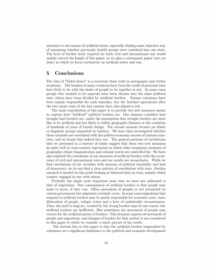
which would have a fractal dimension of 1, versus a line so squiggly that �lls aplane and has a fractal dimension of 2. In practice the fractal measure of actualborders is much closer to 1 than to 2 but there is variation. Figure 1 shows twocountries, Sudan and France. Visually, they are quite di¤erent, as the bordersof Sudan are very straight and those of France are quite squiggly. It will turnout that the fractal dimension for France is 1.0429 and that of Sudan is 1.0245,re�ecting the fact that Sudan�s borders are much closer to being straight lines(dimension 1.0000) than France�s borders.The fractal dimension can be calculated in several ways. We use the box-

count method which is the most straightforward; (Peitgen, Jurgens and Saupe

8

(1992), p 218-219). For this method, a grid of a certain size/scale is projectedonto the border and the number of boxes which the border crosses is tallied.The scale of this grid is also recorded, as measured by the length of a side ofone of the boxes in the grid. This gives a pair of numbers: box-count and box-size. The process is then repeated using grids with di¤erent box-sizes, each timerecording both the box-size and the number of boxes that the border crosses.Given the pairs of data, box-size and box-count, the log-log plot of this datagives the fractal dimension as follows, where the negative of the slope B is thefractal dimension of the line:

ln (box count) = a + b * ln (box size)

Some intuition for this method can be gained by considering two extremecases, a perfectly straight line and a line so wiggly that it covers a whole page(Figure 2a-2d). Figures2a and 2b show two di¤erent grids projected onto aperfectly straight line. The length of the side of a box or the "box size" inFigure 2a is twice that of Figure 2b and we can normalize the box sizes to 2and 1, respectively. Counting the number of squares that the line crosses ineach case, we get a box count of 24 for Figure 2a when the box size is 2, anda box count of 48 for Figure 2b when the box size is 1. Thus, for the straightline, the box count doubles (or increases by a factor of 21) when the box size ishalved (or "increases" by a factor of 2�1). Plotting ln(box count) versus ln(boxsize) yields a downward-sloping line with a slope of �1 (Figure 1g and Table 1). Thus the fractal dimension for the straight line depicted in Figures 2a and2b is determined to be 1. This makes sense because the fractal dimension isidentical to our normal notion of dimension for perfectly straight lines, planesand other simple shapes.Next consider Figures 2c and 2d, which show a line so squiggly that it covers

the whole page. Here the box count is 176 when the box size is 2 (Figure 2c)and the box count is 704 when the box size is 1 (Figure 2d). Thus the box countquadruples (increases by a factor of 22) when the box size is halved ("increases"by a factor of 2�1). In this case, the plot of ln(box count) versus ln(box size)yields a downward-sloping line with a slope of 2 / �1 = �2 (Figure 2g and Table1). Consequently, for this line, which is so squiggly that it �lls the whole page,the fractal dimension is 2. This is also in agreement with the standard notionof dimension in which a plane or a page has two dimensions.The borders of countries will be in between these two extremes of a perfectly

straight line with fractal dimension 1 and a very squiggly line which �lls a wholepage and has a fractal dimension of 2. Consider the somewhat less squiggly linein Figures 2e and 2f. Here, when we calculate the fractal dimension using thebox counting method, we �nd that the box count increases from 54 (Figure2e) to 130 (Figure 2f) when the box size is reduced from 2 to 1, respectively.Thus the box count is more than doubling when the box size is halved. But yetthe box count is not quadrupling, as was the case with the very squiggly line(Figures 2c and 2d). We would thus expect that a plot of ln(box count) versusln(box size) would have a slope that is steeper than -1 but not quite a steep

9

as -2. In fact, when we do the calculation for this example, the slope is -1.267(Figure 2g and Table 1). Based on this result, we would a sign a fractal numberof 1.267 to this squiggly line. In practice the fractal dimension of most countryborders is between 1.000 and 1.100. Squiggly borders have fractal dimensionscloser to 1.100, while straighter borders have fractal dimensions closer to 1.000.These examples use only two data points to determine the fractal dimension

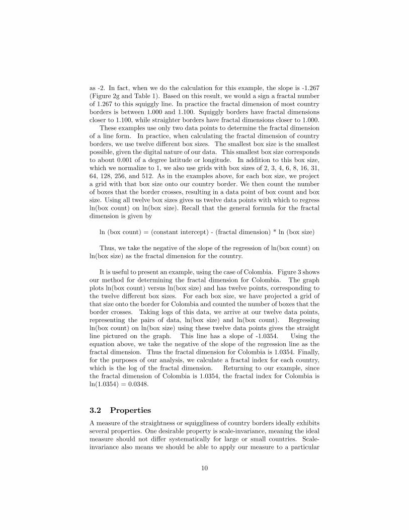
of a line form. In practice, when calculating the fractal dimension of countryborders, we use twelve di¤erent box sizes. The smallest box size is the smallestpossible, given the digital nature of our data. This smallest box size correspondsto about 0.001 of a degree latitude or longitude. In addition to this box size,which we normalize to 1, we also use grids with box sizes of 2, 3, 4, 6, 8, 16, 31,64, 128, 256, and 512. As in the examples above, for each box size, we projecta grid with that box size onto our country border. We then count the numberof boxes that the border crosses, resulting in a data point of box count and boxsize. Using all twelve box sizes gives us twelve data points with which to regressln(box count) on ln(box size). Recall that the general formula for the fractaldimension is given by

ln (box count) = (constant intercept) - (fractal dimension) * ln (box size)

Thus, we take the negative of the slope of the regression of ln(box count) onln(box size) as the fractal dimension for the country.

It is useful to present an example, using the case of Colombia. Figure 3 showsour method for determining the fractal dimension for Colombia. The graphplots ln(box count) versus ln(box size) and has twelve points, corresponding tothe twelve di¤erent box sizes. For each box size, we have projected a grid ofthat size onto the border for Colombia and counted the number of boxes that theborder crosses. Taking logs of this data, we arrive at our twelve data points,representing the pairs of data, ln(box size) and ln(box count). Regressingln(box count) on ln(box size) using these twelve data points gives the straightline pictured on the graph. This line has a slope of -1.0354. Using theequation above, we take the negative of the slope of the regression line as thefractal dimension. Thus the fractal dimension for Colombia is 1.0354. Finally,for the purposes of our analysis, we calculate a fractal index for each country,which is the log of the fractal dimension. Returning to our example, sincethe fractal dimension of Colombia is 1.0354, the fractal index for Colombia isln(1.0354) = 0.0348.

3.2 Properties

A measure of the straightness or squiggliness of country borders ideally exhibitsseveral properties. One desirable property is scale-invariance, meaning the idealmeasure should not di¤er systematically for large or small countries. Scale-invariance also means we should be able to apply our measure to a particular

10

country and get consistent results regardless of the scale of the analysis for thatcountry. Our measure is indeed scale invariant.6

A second desirable property of a �squiggliness� measure is the degree towhich it measures larger-scale irregularities as opposed to smaller-scale irreg-ularities. Small-scale deviations from a smooth curve or line may well be theresult of how ethnic considerations or other local politics determined whether aparticular parcel of land should be on one side of a border or another. Since weare interested in comparing borders where local and ethnic considerations weretaken into account, with more "arti�cial" borders, we prefer our measure to fo-cus on these small-scale irregularities, rather than measuring the overall shapeof a country. Unlike measures such as this circumscribed/inscribed circle ratio,the fractal measure emphasizes the small-scale variation that we are interestedin measuring.We also prefer a measure that treats straight lines and very smooth but

slowly curving lines as similar. Most arbitrarily-drawn borders are straight lines,but we are also interested in a continuum of less-to-more-meandering borders,none of which are perfectly straight lines. Given this, it would be good to avoida discontinuous change in our measure when moving from a rectangular shapeto a smoothly curved shape. As it turns out, there is no discontinuity in thefractal measure, when moving from a perfectly straight line to a smooth curve.Finally, and most importantly, we would like a measure which allows us to

consider only part of the border at a time. In particular, we will disregardcoastlines, since they are determined by nature and not by politics, and may behighly non-compact. The fractal measure can be applied to selected portionsof the border, such as just the political boundaries. Most other measures ofcompactness must use the entire boundary, including coastlines. For instanceother common compactness measures include: the ratio of the longest axis tothe maximum perpendicular length; the ratio of the minimum shape diameterto the maximum diameter; various ratios among the area of the shape, the areaof an inscribing circle and the area of a circumscribing circle; the moment ofinertia of the shape; and the ratio of the area of the shape to the area of a circlewith the same perimeter.7 All of these measures require a closed shape in orderto be calculated.

6To be precise our measure is not 100 percent scale invariant, but it is close to scaleinvarient. Analyzing a country when at di¤ering degrees of being �zoomed in� or �zoomedout�may yield slightly di¤erent values for the fractal dimension. However, these numbers donot vary greatly for each county and the relative rankings of countries are maintained. Moreimportantly, our measure allows us to consistently compare large and small countries. Byusing the same set of 12 box-sizes (as measured in degrees latitude and longitude) for eachcountry, our analysis for each country is on the same �human�scale as for the other countries.By contrast other measures of compactness, such as the ratio of the area of a circumscribedand an inscribed circle for the country border, may di¤er systematically for large and smallcountries.

7For more on this, see Niemi, Grofman, Carlucci, and Hofeller. (1990) and Flaherty, andCrumplin. (1992).

11

3.3 Partitioned groups and other measures

Our second new measure focus on the speci�c issue of borders cutting across anethnic group and dividing it into two adjacent countries. This variable is de�nedas the percent of the population of a country that belongs to a partitioned group.In turn, a partitioned group is one that appear in two or more adjacent countries.One possible objection to this variable is mobility of people. If members ofthe same ethnic groups wanted to be together they could move into the samecountry. However mobility of people is often not free and many countries mayprevent entry (or in some cases exit). We calculate the fractal variable for 144non-island countries. Islands have no political boundaries, so they cannot havea political boundary fractal dimension. The partitioned variable is calculatedfor 131 countries, including 117 countries for which both indices are available.The literature of ethno linguistic fractionalization has normally focused on

one index of fractionalization, the Her�ndhal index which captures the proba-bility that two randomly drawn individuals from the population of the countrybelong to di¤erent groups.8 The original index was based on a linguistic classi-�cation of groups from a Soviet source (Atlas Narodv Mira). It was originallyused in the economic development literature by Mauro (1995) Easterly andLevine (1997) and it is if often referred to as Elf (Ethnolinguistic fractionaliza-tion) index. Alesina and al. (2003) proposed another index that in additionto linguistic di¤erences includes di¤erences based on other characteristic suchas skin color. They label it Frcat but to avoid confusion we label is in thepresent paper Elfn1(See Alesina and al. (2003) for more discussion about theconstruction of this variable)How do our new measures, FRACTAL and PARTITIONED, relate to each

other and to the previously used index of fractionalization? Our fractal measureis meant to capture a much broader idea than ethnic fractionalization. However,arti�cial states as proxied by our measure may end up including di¤erent ethnicgroups within the same political borders, and therefore there should be somecorrelation between the Her�ndhal index of fractionalization and our fractalmeasure. Similar consideration apply for the portioned variable.Table 2 displays the correlation coe¢ cients between the two measures of

arti�cial borders and the more traditional measure of ethnolinguistic fraction-alization. Several comments are in order. First note how the partition variableis positively correlated with the index of ethnic fractionalization, but the corre-lation is in the order of 0.5 so clearly these are "di¤erent variables". Given theway the two variables are constructed it is not surprising that they are positivelycorrelated but they indeed capture di¤erent things. Second the fractal variableis correlated with the Elf and Elf1 measures (with the appropriate negative sign,less curvy borders is associated with more fractionalization), but the correla-tion is not very high especially with Elf, while it is -0.22 with Elf1. Third thecorrelation between our partitioned variable and our fractal variable is basicallyzero. This was frankly a surprise to us. It suggests arti�cial states are noteasy to summarize with one measure. (For example, the partitioned variable

8Another index frequenlty used is a polarization index suggested by RRRR

12

captures only one of the problematic features of arti�cial states mentioned inthe introduction.) We use both measures as providing independent informa-tion on "arti�ciality." Finally, Elf and Elf1 are highly correlated but are notstatistically identical. In summary are two new measure are di¤erent from eachother and are not very highly correlated with other measures previously used inthe literature of ethnic fractionalization.

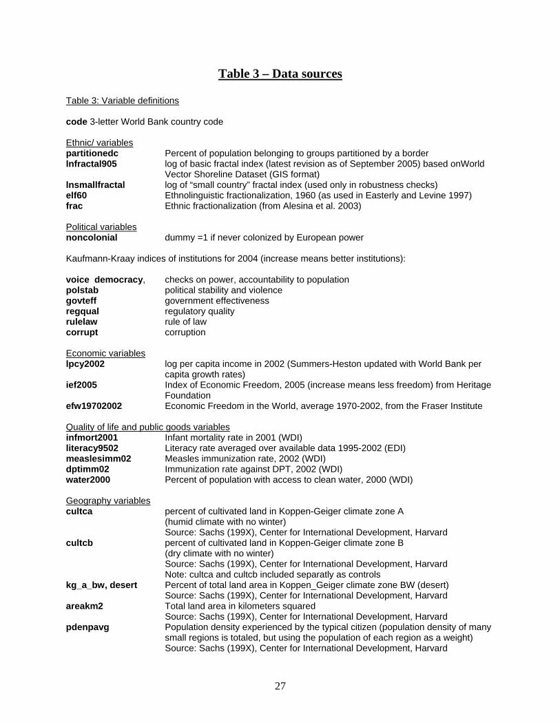
3.4 Data and sources

Data for determining the fractal dimension for each country�s political boundarycomes from the GIS (Geographic Information Systems) format data set WorldVector Shoreline. This data set is the largest scale digital data set of politicalboundaries available today. The data is based on work done by the U.S. mili-tary in the early 1990�s. The non-coastline borders for each country are isolatedusing ArcGIS software9 . This data is then changed to a raster (digitized) for-mat and then to a �tif� format. With a few minor modi�cations, the softwareprogram ImageJ 10 calculates the box-count/ box-size data for twelve di¤erentbox-sizes; the smallest box-size corresponds to the smallest scale of the rasterdata exported from GIS (approximately 0.001 degrees latitude or longitude). Afractal dimension is calculated for each country using this data, ranging from1.000 to 1.100. Finally, we take logs of the fractal dimension to achieve a fractalindex, which ranges from 0 to 0.10.

4 Empirical results

4.1 Which states are "arti�cial"?

Table 3 lists our measures for all the countries in our sample. To illustrate whichstates are most arti�cial according to both measures, we took countries thatwere in the top third of PARTITIONED and in the bottom third of FRACTAL(the straightest borders). Given the weak correlation between the two measures,there were not that many countries in both �13 to be exact. These �most arti�-cial�states are Chad, Ecuador, Equatorial Guinea, Eritrea, Guatemala, Jordan,Mali, Morocco, Namibia, Niger, Pakistan, Sudan, and Zimbabwe. These exam-ples accord with what we know of the historical process that led to formationof these states (some of it described above).What about the US and Canada? Their border is a straight line most of the

way, are they arti�cial states ? According to our measures yes they do scorerelatively in terms of how arti�cial they are, which is certainly not consistentwith a view of arti�cial as failed states, One may notice that this a case inwhich borders were drawn before many pole actually moved in. In many ways

9ArcGIS 9.0 Desktop software from ESRI; www.esri.com10Available online at http://rsb.info.nih.gov/ij/download.html and at

http://rsb.info.nih.gov/ij/developer/index.html

13

the same applies to US states: in the west, their borders drawn when they wereclose to deserted are often straight lines. On the contrary borders of East coaststates, drawn earlier with more population are less straight.11

4.2 Economic and Political Success

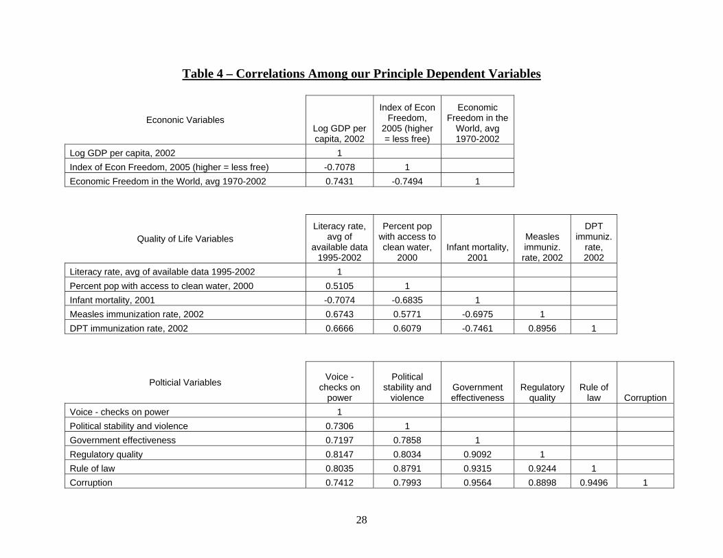
We now turn to verifying whether these new measures of arti�cial states arecorrelated with economic and institutional success. We consider three groupsof variables as left hand side variables. (See Table 3 for variable de�nitionsand sources). First, the variables that measures economic or economic policysuccess: (log of) per capita income in 2002; an index of economic freedom in 2005that measures adherence to a free market economic system; and an alternativeindex of economic freedom averaged over 1970-2002.12 Second, we look atpoltico-institutional variables: voice and accountability (which measure checkson power), political stability and violence, government e¤ectiveness, regulatoryquality, rule of law, and corruption. Third, we use quality of life and publicgoods delivery-related measures: infant mortality in 2001, literacy rate averagedover the period 1995 2002; measles immunization rate in 2002; immunizationrate against DPT in 2002, percent of population with access to clean water, in2000. 13 We choose these variables as representative of state performance inthe core public goods areas of health, education, and infrastructure, selectingparticular measures based on which ones have data available for a large sample ofcountries. All of these variable are clearly correlated with each other. Obviouslyrich country have lower infant mortality, more clean water etc. Table 4 reportsa correlation chart between all of these variables: the correlations are not allvery close to 1 (or -1 depending on the variable de�nition). That is, this set ofvariables do capture di¤erent aspects of politico-economic development that aredi¤erent from each other, so there is information provided by considering all ofthem.Table 5 presents the basic univariate regressions of our measures of arti�cial

states. Consider line one: the left hand side variable is the log of per capita GDPin 2002, and we report only the coe¢ cient and the p value of the single righthand side variable. (Obviously we include also a constant in the regression).Each line represents the same regressions with a di¤erent left hand side variablewhich is listed in the �rst column. We use all the observations available, andtheir number varies (from 84 to 144) in di¤erent regressions because of data

11Needless to say US and Canada are included in our regressions below.12We use the second measure as a robustness check on the �rst measure of economic freedom,

since each is based on a complicated mix of indicators and may re�ect some subjectivity. Giventhe uncertainty surrounding this measure, we also check robustness with respect to using along period average of the second measure rather than just a single year, which may averageout data errors and noise (while sacri�cing our preferred approach of using the most recentdatapoint available).13Data on literacy is spotty, with di¤erent countries reporting di¤erent years over 1995-

2002, so we average all available data over this period. Otherwise, the year given is the mostrecent for which data are widely available.

14

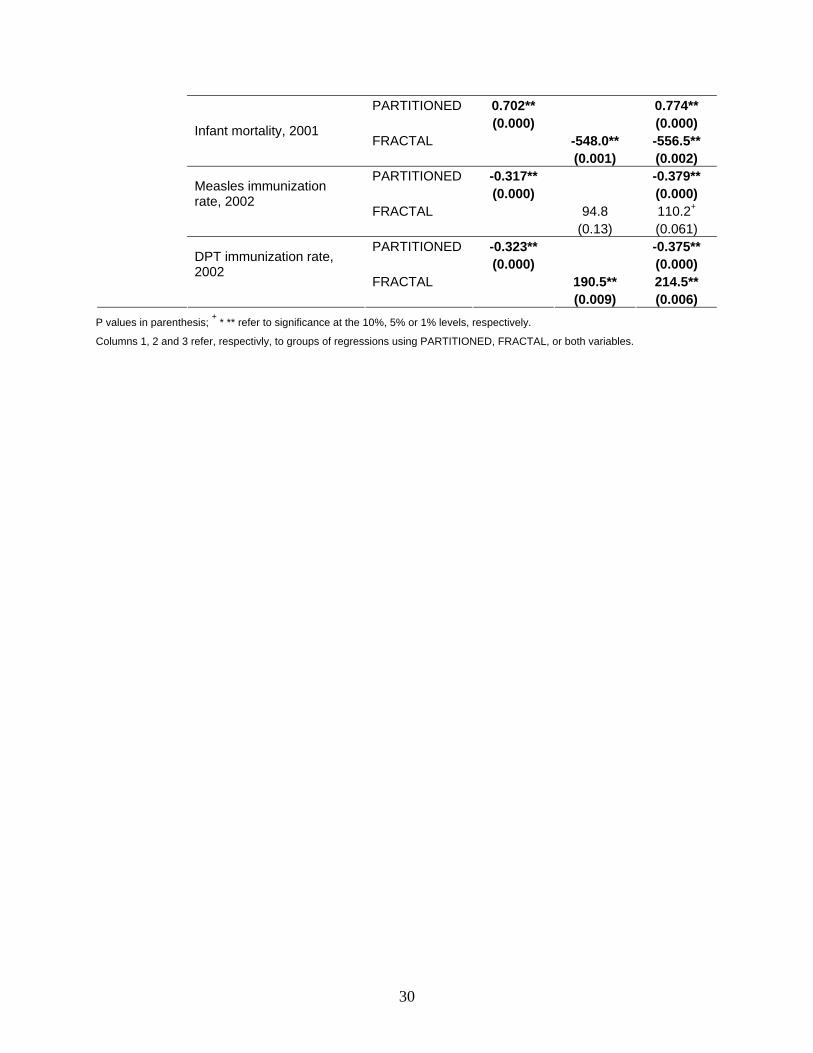
availability on the left hand side variable. The dependent variables are divided inthree blocs: economic variables, institutional variables and quality of life/publicgoods variables. Notice that because of how the right hand side variables areconstructed, we expect the opposite sign in the �rst and second column. So forinstance in the �rst line we expect a negative correlation of economic successmeasured as income per capita in countries where the partition variable assumesa lower value, and in countries where the measure of how straight borders areassumes a higher value. The coe¢ cient in bold represents all the cases in whichstatistical signi�cance (with the expected sign of course) is 5 per cent or better;marginally signi�cant coe¢ cient at the 10 per cent level or better are indicatedwith a "+" sign . Of the 28 coe¢ cients in the �rst two columns, 20 arestatistically signi�cant (5 per cent or better) and there are borderline (p value0.10 or better). Our two measures are not highly correlated with each otherand in fact as discussed above, they capture di¤erent aspects of the nature ofborders. For this reason there is no reason why they could not be used in thesame regressions. In the third column, we use them both. IN all regressionsat least one is signi�cant at the 5 per cent level or better and in almost allregressions they are either both statistically signi�cant at the �ve per cent levelor one is and the other is borderline.Table 6 displays information on the size of the impact of these measures of

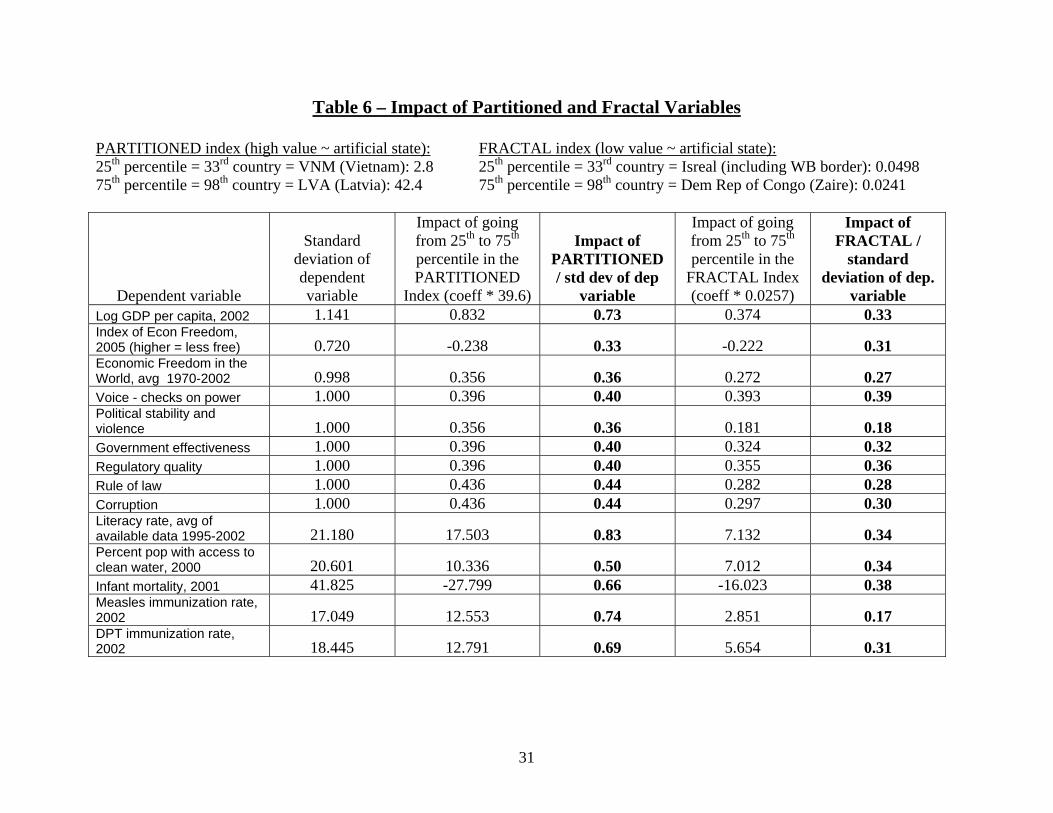
arti�cial states, which is considerable. For the partitioned variable, going fromthe 75th most partitioned country to the 25th most partititioned country isassociated with an increase of 83% in GDP per capita (0.832 log-points; Table6, Column 2). Many of the other variables are also strongly a¤ected, by aroundhalf of a standard deviation (Column 3). The impact of the fractal variable issmaller but still signi�cant in size. Moving from the 75th most squiggly borderto the 25th most squiggly border is associated with a 37% increase in GDP percapita. The other dependent variables are also a¤ected by about a third of astandard deviation.We now check whether these strong univariate correlations survive adding

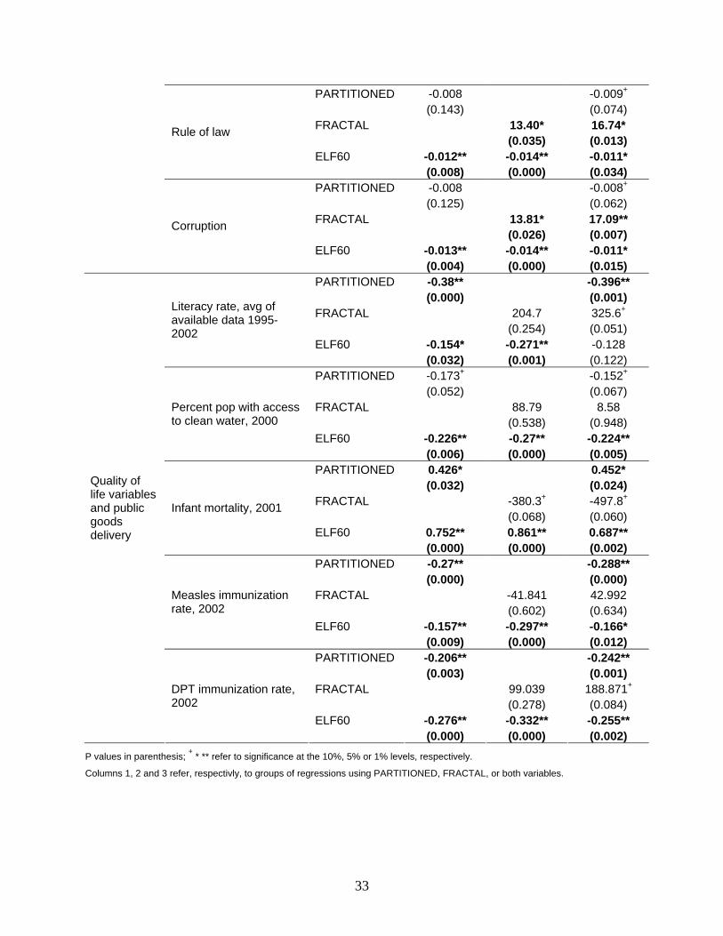
other exogenous variables to the right hand side. We begin with ethnic frac-tionalization to see whether our new measure add anything to traditional andalready used measures of ethic fractionalization. In Table 9 we add as a con-trol in the right hand side the variable ELF, the "traditional" ethnolinguisticfractionalization variable used by Easterly and Levine (1997) and by many afterthem. In the case of our FRACTAL measure, the result suggests that in abouthalf the regressions (6 out of 14) both variables are statistically signi�cant, inanother one FRAXCTAL is marginal at the 10 per cent level . In particular, forthe institutional regressions, FRACTAL remains signi�cant when controllingfor ELF. For the other regressions, ELF is signi�cant but FRACTAL is not.Consider now column 1. Here the variable PARTITIONED remains signi�cantin 7 out of 14 regressions. For GDP per capita, PARTITIONED remains sig-ni�cant when controlling for ELF. Column 3 shows our results when we includeboth variables and control for ELF. Of the 28 coe¢ cients on our arti�cial statesvariables (from the 14 regressions), 16 are signi�cant at a the 5 per cent levelor greater and 9 are borderline at the 10 per cent level.

15

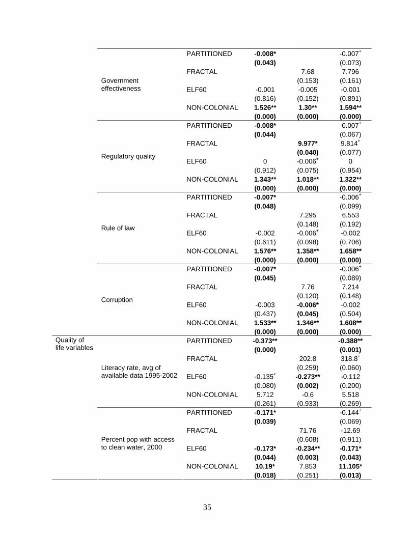
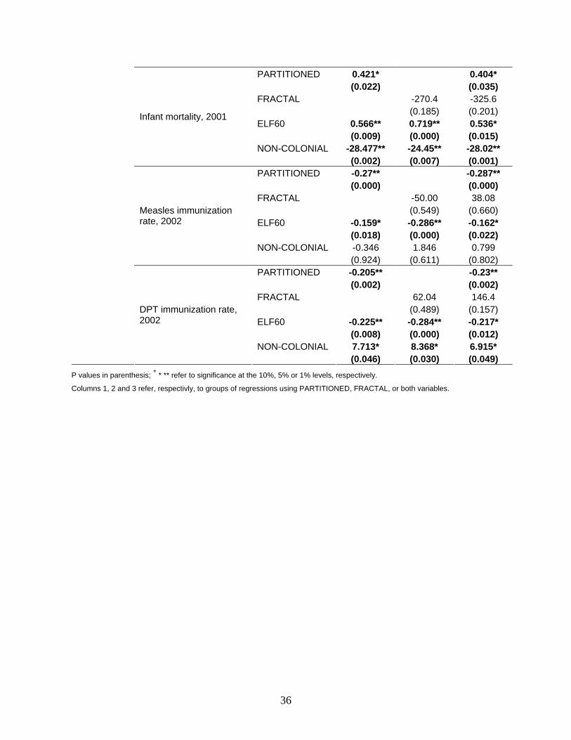
The next experiment is about former colonial status. As we discussed insection 2 above, much of the problem of arti�cial states has to do with colo-nizers drawing borders which did not respect indigenous divisions. In fact, theFRACTAL index for former colonies is lower than for non-former colonies, withthe index averages equal to 0.0335 and 0.0435 for these two groups respectively.This di¤erence is signi�cant at the 1% level. The overall standard deviationfor the fractal index is about 0.02, so this is an important di¤erence of abouthalf a standard deviation between former colonies and non-colonies. Likewise,for the PARTITION variable, former colonies and non-colonies di¤er by 13.6out of the 100 point scale; former colonies have higher proportions citizens from"partitioned" ethnic groups. This di¤erence is also signi�cant at the 1% level.But having been a colony or not may in�uence political and economic outcomesin many di¤erent ways, so it is important to check that controlling for colonialstatus does not change all the signi�cance of our variables of interest. We dothat in Table 8 where we add a dummy variable that assumes the value of 1 ifthe country has never been a colony. In column 1 note how 11 out of the 14coe¢ cients on the partition variable are now signi�cant at the 5 per cent leveland all the others except one are borderline. For the fractal measure, however,only 1 out of 14 is and one is borderline. This show that it is di¢ cult to iden-tify separately the e¤ect of colonial status and straight-line borders, since oneled to the other. For the regressions with both variables, about half of the 28coe¢ cients are signi�cant.Another important exogenous factor that can explain economic and polit-

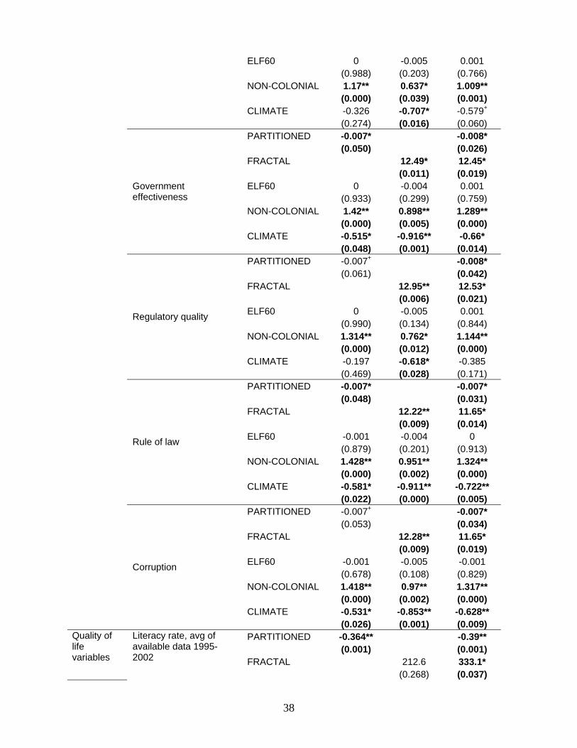
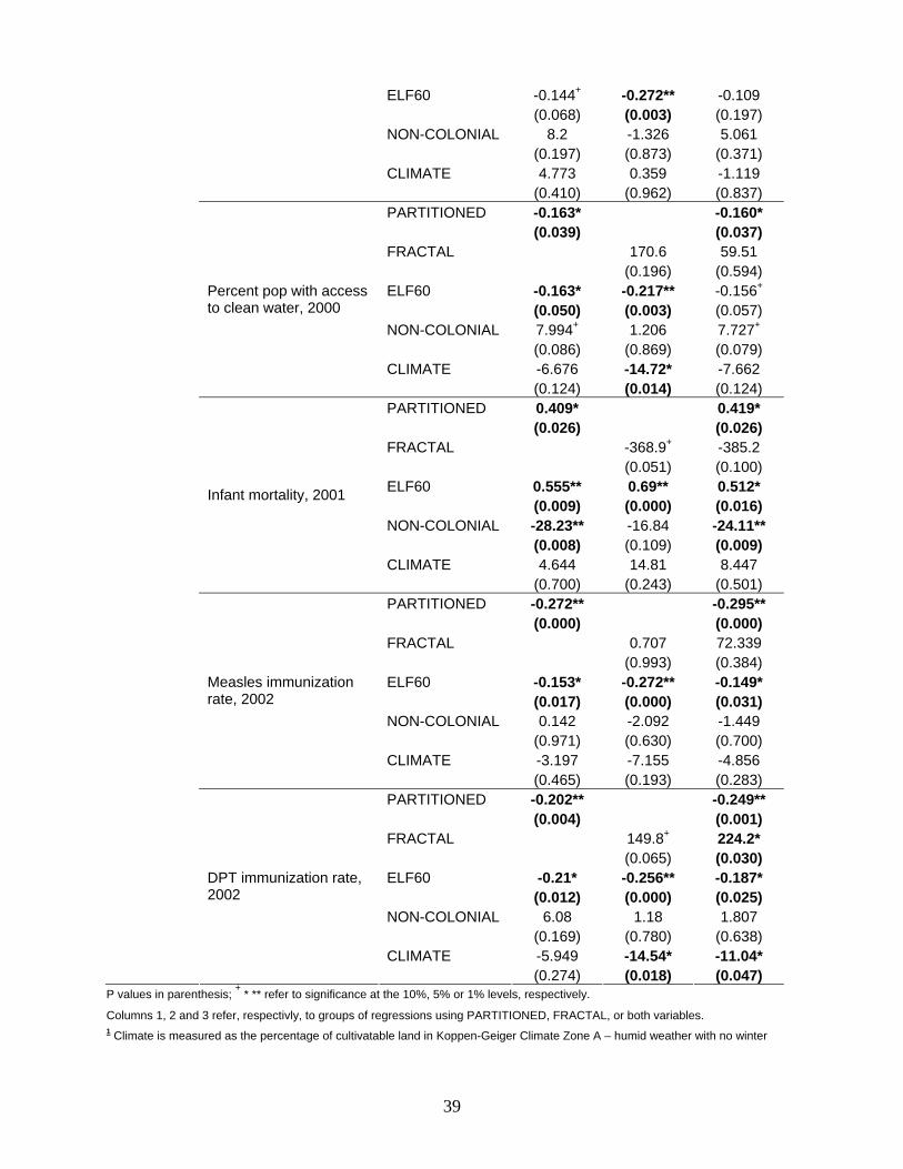
ical success is geography and climate. Many geographic variables have beensuggested in the literature. One of the most precise in capturing weather pat-tern is the variable climate de�ned as the percentage of a country�s cultivatableland that is in the Koppen-Geiger Climate Zone A, which is a humid climatewith no winter. This is a classical de�nition of what constitutes a tropical area.In Table 9 we add this variable to our regression. Our variables are generallyquite robust much more so than the ELF variable.

4.3 Other robustness checks

We consider a number of other possible explanations for our results, addingfurther controls that might otherwise have introduced a spurious correlationwith our measures of arti�ciality of states. In order to keep the length of thispaper manageable, we simply summarize the results here in the text. A separateappendix with the full results will be available on our web sites.

First, we include the index of ethnic fractionalization ELF1, from Alesinaet al. (2003), in place of the control variable ELF. The results are slightly lessstrong, especially for the fractal measure, but the results for GDP and severalhealth indicators remain strong. We then control for the percent of a country�sland area that is desert. Borders may be more likely to be straight in deserts,and desert itself might in�uence our dependent variables of interest. However,controlling for desert leaves our results basically una¤ected.Another possible concern is to what extent our results re�ect outcomes

16

mainly in Africa. We have mixed feelings about introducing an African dummyvariable into our regressions. On one hand, we are concerned that the Africadummy is not truly exogenous because the decision to introduce an Africandummy is in�uenced by the knowledge of poor outcomes in the endogenousvariables in Africa (even the conventional de�nition of Africa as being countriesbelow the Sahara has likely been in�uenced by the di¤ering outcomes in NorthAfrica and sub-Saharan Africa). On the other hand, it is clearly of interestto see whether our results are heavily in�uenced by the sub-Saharan Africanobservations of very arti�cial borders and very poor outcomes. The results arede�nitely weakened by including the Africa dummy, which is always signi�cant.The only result to survive with FRACTAL is for democracy (still signi�cantat the 5 percent level). More of the results on PARTITIONED survive, withthe result on per capita income level, literacy, measles immunization, and DPTimmunization still signi�cant at the 5 percent level, and corruption, clean water,and infant mortality still signi�cant at the 10 percent level.Finally, we control for two other important characteristics of countries that

might be related to the nature of the borders (and thus possibly causing a spu-rious correlation with arti�cial borders): population density and the land areaof the country. Population density is sometimes signi�cant in our regressions,but leaves the results on PARTITIONED and FRACTAL basically unchanged.Land area is often signi�cant and has some e¤ect on the FRACTAL results, butlittle e¤ect on the PARTITIONED results.

4.3.1 Borders and Wars

One type of variable is conspicuously missing in our analysis: wars, both inter-national and civil. Our reason for not discussing it at length is that we foundno e¤ects of arti�cial borders on war. We did �nd an e¤ect of arti�cial borderson a subjective measure of political instability and violence, as described above,but clearly it would be desirable to study the objective outbreaks of wars inaddition to this variable.The lack of an immediate and strong evidence of a correlation between bor-

ders and wars surprised us (although it echoes similar non-results in the liter-ature on ethnic diversity and war). We are not ready to conclude that ethnicrivalries and border disputes are unrelated to wars: we believe that more workis needed. For international war, there is �rst of all the international system(mentioned for Africa in the introduction) that has tended to support existingborders no matter how arti�cial. These international conventions are more bind-ing in some regions than others. Second, to study international wars properly,we need to study pairs of countries and to study to what extent the probabilityof war between them depends on whether the border dividing adjacent ones isarti�cial. There are clearly some examples of border wars arising from partition,such as Israel and its neighbors, India and Pakistan, and Eritrea and Ethiopia.To what extent these examples are validated by a systematic association requiresa study that uses pairwise data on war outbreaks that is beyond the scope ofthis paper. For civil wars, a more detailed analysis would also require some

17

attention to the nature of arti�cial states, especially �nding some objective wayof measuring whether previously hostile groups were combined into one state.The level of further work required for both civil and international war wouldunduly extend the length of this paper, so we plan a subsequent paper (not yetdone) in which we focus exclusively on arti�cial states and war.

5 Conclusions

The idea of "failed states" is a recurrent them both in newspapers and withinacademia. The borders of many countries have been the result of processes thathave little to do with the desire of people to be together or not. In some casesgroups who wanted to be separate have been thrown into the same politicalunit; others have been divided by arti�cial borders. Former colonizers havebeen mainly responsible for such mistakes, but the botched agreements afterthe two major wars of the last century have also played a role.The main contribution of this paper is to provide two new measures meant

to capture how "arti�cial" political borders are. One measure considers howstraight land borders are, under the assumption that straight borders are morelike to be arti�cial and less likely to follow geographic features or the evolutionof hundreds of years of border design. The second measure focuses on ethnicor linguistic groups separated by borders. We have then investigated whetherthese variables are correlated with the politico-economic success of various coun-tries, and we found that indeed they are. The general patterns of correlationsthat we presented in a battery of tables suggest that these two new measuresdo quite well in cross-country regressions in which other exogenous measures ofgeography, ethnic fragmentation and colonial status are controlled for. We havealso explored the correlation of our measures of arti�cial borders with the occur-rence of civil and international wars and our results are inconclusive. While we�nd correlations of our variables with measure of political instability and lackof democracy, we do not �nd a clear pattern of correlations with wars. Furtherresearch is needed on this point looking at bilateral data on wars, namely whichcountry engaged in war with whom.Probably the single most important issue that we have not addressed is

that of migrations. One consequences of arti�cial borders is that people maywant to move, if they can. Often movement of peoples is not permitted byvarious government but migration certainly occur. In some cases migrations thatrespond to arti�cial borders may be partly responsible for economic costs, wars,dislocation of people, refugee crises and a hots of undesirable circumstances.Thus, the need to migrate, created by the wrong borders may be one reason whyarti�cial borders are ine¢ cient. But sometimes the movement of people maycorrect for the arti�cial nature of borders. This dynamic aspects of movement ofpeople and migrations, and changes of borders for that matter is not consideredin this paper in which we consider a static picture of the world.

The bottom line in this paper is that the arti�cial borders bequeathed bycolonizers are a signi�cant hindrance to the political and economic development

18

of the independent states that followed the colonies.

6 References

References

[1] Acemoglu Daron, Simon Johnson and James Robinson (2001) " The Colo-nial Origin of Comparative Development: An Empirical Investigation."American Economic Review. v91, p1369-401.

[2] Alcala, Francisco and Antonio Ciccone (2004) "Trade and Productivity."Quarterly Journal of Economics. v119:2, p613-46

[3] Alesina, Alberto, Arnaud Devleeschauwer, William Easterly, Sergio Kurlat,and Romain Wacziarg (2003) "Fractionalization." Journal of EconomicGrowth, 8, 155-94.

[4] Alesina, Alberto and Enrico Spolaore (1997) "On the Number and Size ofNations." Quarterly Journal of Economics. v112, p1027-56

[5] Alesina, Alberto and Enrico Spolaore (2003) The Size of Nations. Cam-bridge MA: MIT Press.

[6] Alesina, Alberto, Enrico Spolaore and Romain Wacziarg(2000) "EconomicIntegration and Political Disintegration." American Economic Review. v90,p1276-96

[7] Bourke, P. (1993) Fractal Dimension Cal-culator User Manual, Online. Available:http://astronomy.swin.edu.au/~pbourke/fractals/fracdim/fdc_orig/

[8] Bruk, S. I., and V.S. Apenchenko (eds.) (1964) Atlas Narodov Mira.Moscow: Glavnoe Upravlenie Geodezii i Kartogra�i.

[9] ATLAS NARODOV MIRA [ATLAS OF THE PEOPLES OF THEWORLD]. Moscow: Glavnoe Upravlenie Geodezii i Kartogra�i, 1964.

[10] Easterly, William. (2006) The White Man�s Burden: Why the West�s Ef-forts to Aid the Rest Did So Much Harm and So Little Good. New York:The Penguin Press.

[11] Easterly, William and Ross Levine (1997) "Africa�s Growth Tragedy: Poli-cies and Ethnic Divisions." Quarterly Journal of Economics. v112:4, p1203-50

[12] Englebert, Peter, Stacy Tarango and Matther Carter (2002) "Dismember-ment and Su¤ocation: A Contribution to the Debate on African Bound-aries." Comparative Political Studies. v35:10, p1093-1118

19

[13] Flaherty, Mark S. and William W. Crumplin. (1992) "Compactness andElectoral Boundary Adjustment: An Assessment of Alternative Measures."The Canadian Geographer v36:2, p159-171

[14] Glaeser Edward Rafael La Porta, Florencio Lopez de Silanes and An-drei Shleifer (2004)"Do Institutions Cause Growth?" Jornal of EconomicGrowth, 271-303.

[15] La Porta Rafael , Florencio Lopez de Silanes, Andrei Shleifer and RobertVishny (1999) "The Quality of Government" Journal of Law Economicsand Organization, 315 388.

[16] Mandelbrot, Beniot. (1967) "How Long is the Coast of Britain? StatisticalSelf-Similarity and Fractional Dimension." Science. New Series v156, p636-638.

[17] Mauro, Paolo (1995) "Corruption and Growth." Quarterly Journal of Eco-nomics. v110:3, p681-712.

[18] Mc Millan Margaret (2003) "Paris 1919"

[19] Herbst Je¤rey (2002) State and Power in Africa. Princeton, NJ: PrincetonUniversity Press.

[20] Niemi, Richard G., Bernard Grofman, Carl Carlucci, and Thomas Hofeller.(1990) "Measuring Compactness and the Role of a Compactness Standardin a Test for Partisan and Racial Gerrymandering." Journal of Politics.v52:4, p1155-1181

[21] Peitgen, Heinz-Otto, Hartmut Jurgens and Dietmar Saupe (1992). Chaosand Fractals; New Frontiers of Science. New York: Springer-Verlag.

[22] Van Der Veen, Roel. (2004) What Went Wrong With Africa: A Contem-porary History. Amsterdam: KIT Publishers.

[23] Winn, Peter. (1992) Americas: The Changing Face of Latin America andthe Caribbean. New York: Pantheon Books.

20

Figure 1 – Artificial versus Organic boundaries – Sudan and France

Figure 1a – France, with poltical boundaries highlighted at left

Figure 1b – Sudan, with poltical boundaries highlighted at left

France Fractal dimension of political boundary = 1.0429

Fractal n of

Sudan

dimensiopolitical boundary = 1.0245

21

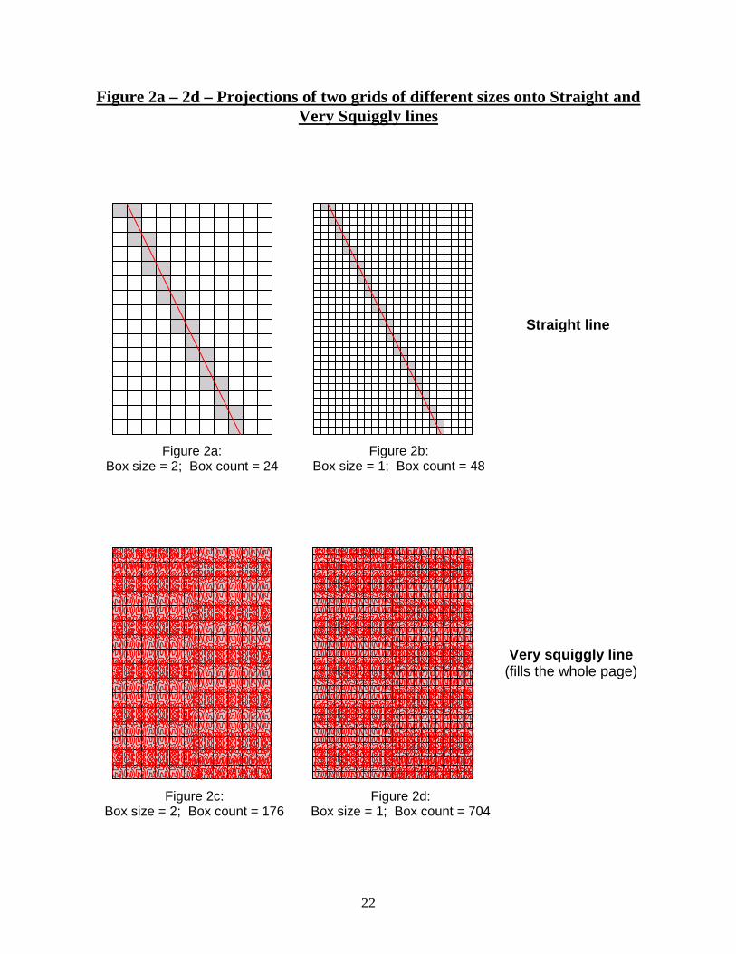
Figure 2a – 2d – Projections of two grids of different sizes onto Straight and Very Squiggly lines

Figure 2b: Box size = 1; Box count = 48

Straight line

Figure 2a: Box size = 2; Box count = 24

Figure 2c: Box size = 2; Box count = 176

Figure 2d: Box size = 1; Box count = 704

Very squiggly line (fills the whole page)

22

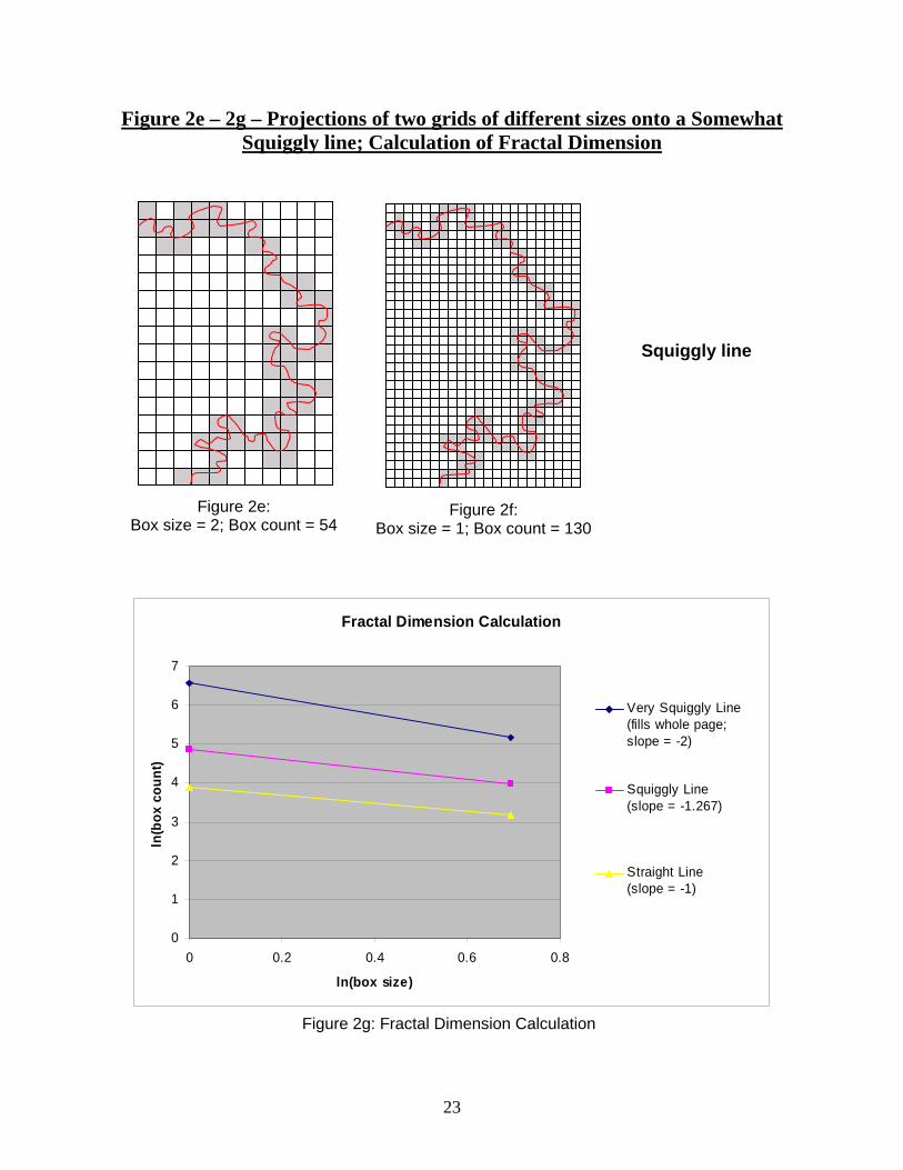
Figure 2e – 2g – Projections of two grids of different sizes onto a Somewhat Squiggly line; Calculation of Fractal Dimension

Figure 2e: Box size = 2; Box count = 54

Squiggly line

Figure 2f: Box size = 1; Box count = 130

Fractal Dimension Calculation

0

1

2

3

4

5

6

7

0 0.2 0.4 0.6 0.8

ln(box size)

ln(b

ox c

ount

)

Very Squiggly Line(fills whole page;slope = -2)

Squiggly Line(slope = -1.267)

Straight Line(slope = -1)

Figure 2g: Fractal Dimension Calculation

23

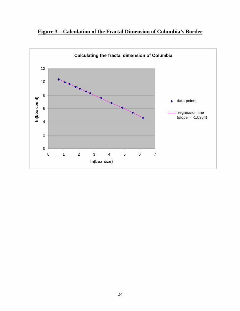
Figure 3 – Calculation of the Fractal Dimension of Columbia’s Border

Calculating the fractal dimension of Columbia

0

2

4

6

8

10

12

0 1 2 3 4 5 6 7

ln(box size)

ln(b

ox c

ount

)

data points

regression line (slope = -1.0354)

24

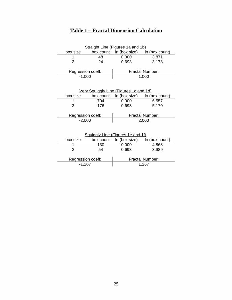
Table 1 – Fractal Dimension Calculation

Straight Line (Figures 1a and 1b)

box size box count ln (box size) ln (box count) 1 48 0.000 3.871 2 24 0.693 3.178

Regression coeff: Fractal Number: -1.000 1.000

Very Squiggly Line (Figures 1c and 1d) box size box count ln (box size) ln (box count)

1 704 0.000 6.557 2 176 0.693 5.170


Squiggly Line (Figures 1e and 1f) box size box count ln (box size) ln (box count)

1 130 0.000 4.868 2 54 0.693 3.989


25

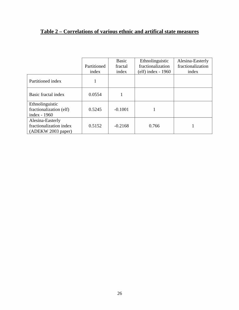
Table 2 – Correlations of various ethnic and artifical state measures

Partitioned

index

Basic fractal index

Ethnolinguistic fractionalization (elf) index - 1960

Alesina-Easterly fractionalization

index

Partitioned index 1

Basic fractal index 0.0554 1

Ethnolinguistic fractionalization (elf) index - 1960

0.5245 -0.1001 1

Alesina-Easterly fractionalization index (ADEKW 2003 paper)

0.5152 -0.2168 0.766 1

26

27

Table 3 – Data sources

Table 3: Variable definitions code 3-letter World Bank country code Ethnic/ variables partitionedc Percent of population belonging to groups partitioned by a border lnfractal905 log of basic fractal index (latest revision as of September 2005) based onWorld Vector Shoreline Dataset (GIS format) lnsmallfractal log of “small country” fractal index (used only in robustness checks) elf60 Ethnolinguistic fractionalization, 1960 (as used in Easterly and Levine 1997) frac Ethnic fractionalization (from Alesina et al. 2003) Political variables noncolonial dummy =1 if never colonized by European power Kaufmann-Kraay indices of institutions for 2004 (increase means better institutions): voice democracy, checks on power, accountability to population polstab political stability and violence govteff government effectiveness regqual regulatory quality rulelaw rule of law corrupt corruption Economic variables lpcy2002 log per capita income in 2002 (Summers-Heston updated with World Bank per

capita growth rates) ief2005 Index of Economic Freedom, 2005 (increase means less freedom) from Heritage

Foundation efw19702002 Economic Freedom in the World, average 1970-2002, from the Fraser Institute Quality of life and public goods variables infmort2001 Infant mortality rate in 2001 (WDI) literacy9502 Literacy rate averaged over available data 1995-2002 (EDI) measlesimm02 Measles immunization rate, 2002 (WDI) dptimm02 Immunization rate against DPT, 2002 (WDI) water2000 Percent of population with access to clean water, 2000 (WDI) Geography variables cultca percent of cultivated land in Koppen-Geiger climate zone A (humid climate with no winter) Source: Sachs (199X), Center for International Development, Harvard cultcb percent of cultivated land in Koppen-Geiger climate zone B (dry climate with no winter) Source: Sachs (199X), Center for International Development, Harvard Note: cultca and cultcb included separatly as controls kg_a_bw, desert Percent of total land area in Koppen_Geiger climate zone BW (desert) Source: Sachs (199X), Center for International Development, Harvard areakm2 Total land area in kilometers squared Source: Sachs (199X), Center for International Development, Harvard pdenpavg Population density experienced by the typical citizen (population density of many small regions is totaled, but using the population of each region as a weight) Source: Sachs (199X), Center for International Development, Harvard

28

Table 4 – Correlations Among our Principle Dependent Variables

Econonic Variables Log GDP per capita, 2002

Index of Econ Freedom,

2005 (higher = less free)

Economic Freedom in the

World, avg 1970-2002

Log GDP per capita, 2002 1 Index of Econ Freedom, 2005 (higher = less free) -0.7078 1 Economic Freedom in the World, avg 1970-2002 0.7431 -0.7494 1

Quality of Life Variables Literacy rate,

avg of available data

1995-2002

Percent pop with access to clean water,

2000 Infant mortality,

2001

Measles immuniz. rate, 2002

DPT immuniz.

rate, 2002

Literacy rate, avg of available data 1995-2002 1 Percent pop with access to clean water, 2000 0.5105 1 Infant mortality, 2001 -0.7074 -0.6835 1 Measles immunization rate, 2002 0.6743 0.5771 -0.6975 1 DPT immunization rate, 2002 0.6666 0.6079 -0.7461 0.8956 1

Polticial Variables Voice - checks on

power

Political stability and

violence Government effectiveness

Regulatory quality

Rule of law Corruption

Voice - checks on power 1 Political stability and violence 0.7306 1 Government effectiveness 0.7197 0.7858 1 Regulatory quality 0.8147 0.8034 0.9092 1 Rule of law 0.8035 0.8791 0.9315 0.9244 1 Corruption 0.7412 0.7993 0.9564 0.8898 0.9496 1

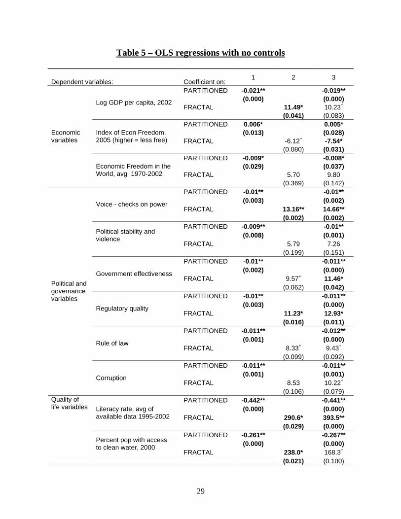
Table 5 – OLS regressions with no controls

Dependent variables: Coefficient on: 1 2 3

PARTITIONED -0.021** -0.019** (0.000) (0.000) FRACTAL 11.49* 10.23+Log GDP per capita, 2002

(0.041) (0.083) PARTITIONED 0.006* 0.005* (0.013) (0.028) FRACTAL -6.12+ -7.54*

Index of Econ Freedom, 2005 (higher = less free)

(0.080) (0.031) PARTITIONED -0.009* -0.008* (0.029) (0.037) FRACTAL 5.70 9.80

Economic variables

Economic Freedom in the World, avg 1970-2002

(0.369) (0.142) PARTITIONED -0.01** -0.01** (0.003) (0.002) FRACTAL 13.16** 14.66**

Voice - checks on power

(0.002) (0.002) PARTITIONED -0.009** -0.01** (0.008) (0.001) FRACTAL 5.79 7.26

Political stability and violence

(0.199) (0.151) PARTITIONED -0.01** -0.011** (0.002) (0.000) FRACTAL 9.57+ 11.46*

Government effectiveness

(0.062) (0.042) PARTITIONED -0.01** -0.011** (0.003) (0.000) FRACTAL 11.23* 12.93*

Regulatory quality

(0.016) (0.011) PARTITIONED -0.011** -0.012** (0.001) (0.000) FRACTAL 8.33+ 9.43+Rule of law

(0.099) (0.092) PARTITIONED -0.011** -0.011** (0.001) (0.001) FRACTAL 8.53 10.22+

Political and governance variables

Corruption

(0.106) (0.079) PARTITIONED -0.442** -0.441** (0.000) (0.000) FRACTAL 290.6* 393.5**

Literacy rate, avg of available data 1995-2002

(0.029) (0.000) PARTITIONED -0.261** -0.267** (0.000) (0.000) FRACTAL 238.0* 168.3+

Quality of life variables

Percent pop with access to clean water, 2000

(0.021) (0.100)

29

30

PARTITIONED 0.702** 0.774** (0.000) (0.000) FRACTAL -548.0** -556.5**

Infant mortality, 2001

(0.001) (0.002) PARTITIONED -0.317** -0.379** (0.000) (0.000) FRACTAL 94.8 110.2+

Measles immunization rate, 2002

(0.13) (0.061) PARTITIONED -0.323** -0.375** (0.000) (0.000) FRACTAL 190.5** 214.5**

DPT immunization rate, 2002

(0.009) (0.006)

P values in parenthesis; + * ** refer to significance at the 10%, 5% or 1% levels, respectively.

Columns 1, 2 and 3 refer, respectivly, to groups of regressions using PARTITIONED, FRACTAL, or both variables.

31

Table 6 – Impact of Partitioned and Fractal Variables

PARTITIONED index (high value ~ artificial state): FRACTAL index (low value ~ artificial state):25th percentile = 33rd country = VNM (Vietnam): 2.8 25th percentile = 33rd country = Isreal (including WB border): 0.0498 75th percentile = 98th country = LVA (Latvia): 42.4 75th percentile = 98th country = Dem Rep of Congo (Zaire): 0.0241

Dependent variable

Standard deviation of dependent variable

Impact of going from 25th to 75th percentile in the PARTITIONED

Index (coeff * 39.6)

Impact of PARTITIONED / std dev of dep

variable

Impact of going from 25th to 75th percentile in the

FRACTAL Index (coeff * 0.0257)

Impact of FRACTAL /

standard deviation of dep.

variable Log GDP per capita, 2002 1.141 0.832 0.73 0.374 0.33 Index of Econ Freedom, 2005 (higher = less free) 0.720 -0.238 0.33 -0.222 0.31 Economic Freedom in the World, avg 1970-2002 0.998 0.356 0.36 0.272 0.27 Voice - checks on power 1.000 0.396 0.40 0.393 0.39 Political stability and violence 1.000 0.356 0.36 0.181 0.18 Government effectiveness 1.000 0.396 0.40 0.324 0.32 Regulatory quality 1.000 0.396 0.40 0.355 0.36 Rule of law 1.000 0.436 0.44 0.282 0.28 Corruption 1.000 0.436 0.44 0.297 0.30 Literacy rate, avg of available data 1995-2002 21.180 17.503 0.83 7.132 0.34 Percent pop with access to clean water, 2000 20.601 10.336 0.50 7.012 0.34 Infant mortality, 2001 41.825 -27.799 0.66 -16.023 0.38 Measles immunization rate, 2002 17.049 12.553 0.74 2.851 0.17 DPT immunization rate, 2002 18.445 12.791 0.69 5.654 0.31

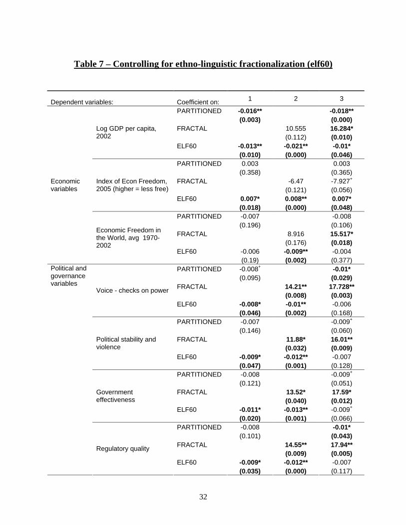
Table 7 – Controlling for ethno-linguistic fractionalization (elf60)


PARTITIONED -0.016** -0.018** (0.003) (0.000) FRACTAL 10.555 16.284* (0.112) (0.010) ELF60 -0.013** -0.021** -0.01*

Log GDP per capita, 2002

(0.010) (0.000) (0.046) PARTITIONED 0.003 0.003 (0.358) (0.365) FRACTAL -6.47 -7.927+

(0.121) (0.056) ELF60 0.007* 0.008** 0.007*


(0.018) (0.000) (0.048) PARTITIONED -0.007 -0.008 (0.196) (0.106) FRACTAL 8.916 15.517* (0.176) (0.018) ELF60 -0.006 -0.009** -0.004

Economic variables


(0.19) (0.002) (0.377) PARTITIONED -0.008+ -0.01* (0.095) (0.029) FRACTAL 14.21** 17.728** (0.008) (0.003) ELF60 -0.008* -0.01** -0.006


(0.046) (0.002) (0.168) PARTITIONED -0.007 -0.009+

(0.146) (0.060) FRACTAL 11.88* 16.01** (0.032) (0.009) ELF60 -0.009* -0.012** -0.007


(0.047) (0.001) (0.128) PARTITIONED -0.008 -0.009+

(0.121) (0.051) FRACTAL 13.52* 17.59* (0.040) (0.012) ELF60 -0.011* -0.013** -0.009+


(0.020) (0.001) (0.066) PARTITIONED -0.008 -0.01* (0.101) (0.043) FRACTAL 14.55** 17.94** (0.009) (0.005) ELF60 -0.009* -0.012** -0.007


Regulatory quality

(0.035) (0.000) (0.117)

32

PARTITIONED -0.008 -0.009+

(0.143) (0.074) FRACTAL 13.40* 16.74* (0.035) (0.013) ELF60 -0.012** -0.014** -0.011*

Rule of law

(0.008) (0.000) (0.034) PARTITIONED -0.008 -0.008+

(0.125) (0.062) FRACTAL 13.81* 17.09** (0.026) (0.007) ELF60 -0.013** -0.014** -0.011*

Corruption

(0.004) (0.000) (0.015) PARTITIONED -0.38** -0.396** (0.000) (0.001) FRACTAL 204.7 325.6+

(0.254) (0.051) ELF60 -0.154* -0.271** -0.128


(0.032) (0.001) (0.122) PARTITIONED -0.173+ -0.152+

(0.052) (0.067) FRACTAL 88.79 8.58 (0.538) (0.948) ELF60 -0.226** -0.27** -0.224**


(0.006) (0.000) (0.005) PARTITIONED 0.426* 0.452* (0.032) (0.024) FRACTAL -380.3+ -497.8+

(0.068) (0.060) ELF60 0.752** 0.861** 0.687**


(0.000) (0.000) (0.002) PARTITIONED -0.27** -0.288** (0.000) (0.000) FRACTAL -41.841 42.992 (0.602) (0.634) ELF60 -0.157** -0.297** -0.166*



(0.278) (0.084) ELF60 -0.276** -0.332** -0.255**

Quality of life variables and public goods delivery


(0.000) (0.000) (0.002)



33

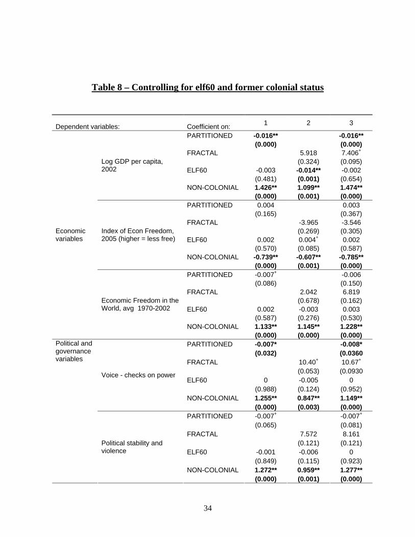
Table 8 – Controlling for elf60 and former colonial status


PARTITIONED -0.016** -0.016** (0.000) (0.000) FRACTAL 5.918 7.406+

(0.324) (0.095) ELF60 -0.003 -0.014** -0.002 (0.481) (0.001) (0.654) NON-COLONIAL 1.426** 1.099** 1.474**


(0.000) (0.001) (0.000) PARTITIONED 0.004 0.003 (0.165) (0.367) FRACTAL -3.965 -3.546 (0.269) (0.305) ELF60 0.002 0.004+ 0.002 (0.570) (0.085) (0.587) NON-COLONIAL -0.739** -0.607** -0.785**


(0.000) (0.001) (0.000) PARTITIONED -0.007+ -0.006 (0.086) (0.150) FRACTAL 2.042 6.819 (0.678) (0.162) ELF60 0.002 -0.003 0.003 (0.587) (0.276) (0.530) NON-COLONIAL 1.133** 1.145** 1.228**

Economic variables


(0.000) (0.000) (0.000) PARTITIONED -0.007* -0.008* (0.032) (0.0360 FRACTAL 10.40+ 10.67+

(0.053) (0.0930 ELF60 0 -0.005 0 (0.988) (0.124) (0.952) NON-COLONIAL 1.255** 0.847** 1.149**


(0.000) (0.003) (0.000) PARTITIONED -0.007+ -0.007+

(0.065) (0.081) FRACTAL 7.572 8.161 (0.121) (0.121) ELF60 -0.001 -0.006 0 (0.849) (0.115) (0.923) NON-COLONIAL 1.272** 0.959** 1.277**



(0.000) (0.001) (0.000)

34

PARTITIONED -0.008* -0.007+

(0.043) (0.073) FRACTAL 7.68 7.796 (0.153) (0.161) ELF60 -0.001 -0.005 -0.001 (0.816) (0.152) (0.891) NON-COLONIAL 1.526** 1.30** 1.594**


(0.000) (0.000) (0.000) PARTITIONED -0.008* -0.007+

(0.044) (0.067) FRACTAL 9.977* 9.814+

(0.040) (0.077) ELF60 0 -0.006+ 0 (0.912) (0.075) (0.954) NON-COLONIAL 1.343** 1.018** 1.322**

Regulatory quality

(0.000) (0.000) (0.000) PARTITIONED -0.007* -0.006+

(0.048) (0.099) FRACTAL 7.295 6.553 (0.148) (0.192) ELF60 -0.002 -0.006+ -0.002 (0.611) (0.098) (0.706) NON-COLONIAL 1.576** 1.358** 1.658**

Rule of law

(0.000) (0.000) (0.000) PARTITIONED -0.007* -0.006+

(0.045) (0.089) FRACTAL 7.76 7.214 (0.120) (0.148) ELF60 -0.003 -0.006* -0.002 (0.437) (0.045) (0.504) NON-COLONIAL 1.533** 1.346** 1.608**

Corruption


(0.259) (0.060) ELF60 -0.135+ -0.273** -0.112 (0.080) (0.002) (0.200) NON-COLONIAL 5.712 -0.6 5.518


(0.261) (0.933) (0.269) PARTITIONED -0.171* -0.144+

(0.039) (0.069) FRACTAL 71.76 -12.69 (0.608) (0.911) ELF60 -0.173* -0.234** -0.171* (0.044) (0.003) (0.043) NON-COLONIAL 10.19* 7.853 11.105*



(0.018) (0.251) (0.013)

35

PARTITIONED 0.421* 0.404* (0.022) (0.035) FRACTAL -270.4 -325.6 (0.185) (0.201) ELF60 0.566** 0.719** 0.536* (0.009) (0.000) (0.015) NON-COLONIAL -28.477** -24.45** -28.02**


(0.002) (0.007) (0.001) PARTITIONED -0.27** -0.287** (0.000) (0.000) FRACTAL -50.00 38.08 (0.549) (0.660) ELF60 -0.159* -0.286** -0.162* (0.018) (0.000) (0.022) NON-COLONIAL -0.346 1.846 0.799


(0.924) (0.611) (0.802) PARTITIONED -0.205** -0.23** (0.002) (0.002) FRACTAL 62.04 146.4 (0.489) (0.157) ELF60 -0.225** -0.284** -0.217* (0.008) (0.000) (0.012) NON-COLONIAL 7.713* 8.368* 6.915*


(0.046) (0.030) (0.049)



36

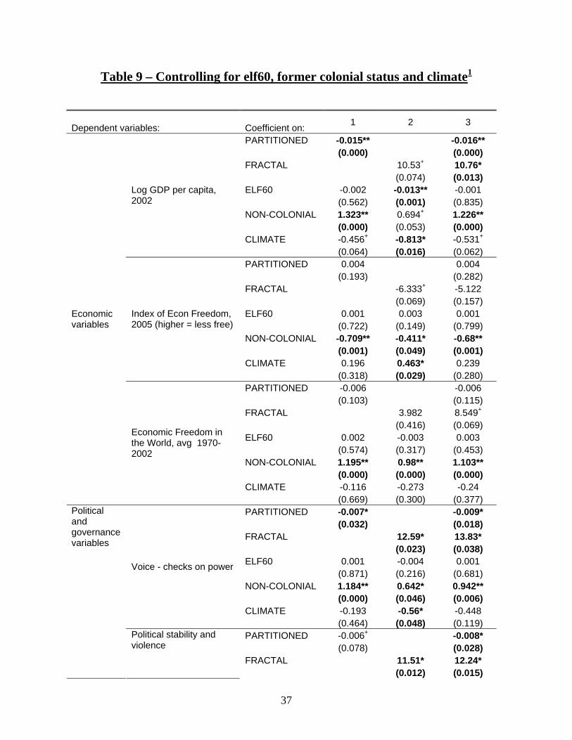
Table 9 – Controlling for elf60, former colonial status and climate1


PARTITIONED -0.015** -0.016** (0.000) (0.000) FRACTAL 10.53+ 10.76* (0.074) (0.013) ELF60 -0.002 -0.013** -0.001 (0.562) (0.001) (0.835) NON-COLONIAL 1.323** 0.694+ 1.226** (0.000) (0.053) (0.000) CLIMATE -0.456+ -0.813* -0.531+


(0.064) (0.016) (0.062) PARTITIONED 0.004 0.004 (0.193) (0.282) FRACTAL -6.333+ -5.122 (0.069) (0.157) ELF60 0.001 0.003 0.001 (0.722) (0.149) (0.799) NON-COLONIAL -0.709** -0.411* -0.68** (0.001) (0.049) (0.001) CLIMATE 0.196 0.463* 0.239


(0.318) (0.029) (0.280) PARTITIONED -0.006 -0.006 (0.103) (0.115) FRACTAL 3.982 8.549+

(0.416) (0.069) ELF60 0.002 -0.003 0.003 (0.574) (0.317) (0.453) NON-COLONIAL 1.195** 0.98** 1.103** (0.000) (0.000) (0.000) CLIMATE -0.116 -0.273 -0.24

Economic variables


(0.669) (0.300) (0.377) PARTITIONED -0.007* -0.009* (0.032) (0.018) FRACTAL 12.59* 13.83* (0.023) (0.038) ELF60 0.001 -0.004 0.001 (0.871) (0.216) (0.681) NON-COLONIAL 1.184** 0.642* 0.942** (0.000) (0.046) (0.006) CLIMATE -0.193 -0.56* -0.448


(0.464) (0.048) (0.119) PARTITIONED -0.006+ -0.008* (0.078) (0.028) FRACTAL 11.51* 12.24*



(0.012) (0.015)

37

ELF60 0 -0.005 0.001 (0.988) (0.203) (0.766) NON-COLONIAL 1.17** 0.637* 1.009** (0.000) (0.039) (0.001) CLIMATE -0.326 -0.707* -0.579+

(0.274) (0.016) (0.060) PARTITIONED -0.007* -0.008* (0.050) (0.026) FRACTAL 12.49* 12.45* (0.011) (0.019) ELF60 0 -0.004 0.001 (0.933) (0.299) (0.759) NON-COLONIAL 1.42** 0.898** 1.289** (0.000) (0.005) (0.000) CLIMATE -0.515* -0.916** -0.66*


(0.048) (0.001) (0.014) PARTITIONED -0.007+ -0.008* (0.061) (0.042) FRACTAL 12.95** 12.53* (0.006) (0.021) ELF60 0 -0.005 0.001 (0.990) (0.134) (0.844) NON-COLONIAL 1.314** 0.762* 1.144** (0.000) (0.012) (0.000) CLIMATE -0.197 -0.618* -0.385

Regulatory quality

(0.469) (0.028) (0.171) PARTITIONED -0.007* -0.007* (0.048) (0.031) FRACTAL 12.22** 11.65* (0.009) (0.014) ELF60 -0.001 -0.004 0 (0.879) (0.201) (0.913) NON-COLONIAL 1.428** 0.951** 1.324** (0.000) (0.002) (0.000) CLIMATE -0.581* -0.911** -0.722**

Rule of law

(0.022) (0.000) (0.005) PARTITIONED -0.007+ -0.007* (0.053) (0.034) FRACTAL 12.28** 11.65* (0.009) (0.019) ELF60 -0.001 -0.005 -0.001 (0.678) (0.108) (0.829) NON-COLONIAL 1.418** 0.97** 1.317** (0.000) (0.002) (0.000) CLIMATE -0.531* -0.853** -0.628**

Corruption

(0.026) (0.001) (0.009) PARTITIONED -0.364** -0.39** (0.001) (0.001) FRACTAL 212.6 333.1*



(0.268) (0.037)

38

ELF60 -0.144+ -0.272** -0.109 (0.068) (0.003) (0.197) NON-COLONIAL 8.2 -1.326 5.061 (0.197) (0.873) (0.371) CLIMATE 4.773 0.359 -1.119 (0.410) (0.962) (0.837) PARTITIONED -0.163* -0.160* (0.039) (0.037) FRACTAL 170.6 59.51 (0.196) (0.594) ELF60 -0.163* -0.217** -0.156+

(0.050) (0.003) (0.057) NON-COLONIAL 7.994+ 1.206 7.727+

(0.086) (0.869) (0.079) CLIMATE -6.676 -14.72* -7.662


(0.124) (0.014) (0.124) PARTITIONED 0.409* 0.419* (0.026) (0.026) FRACTAL -368.9+ -385.2 (0.051) (0.100) ELF60 0.555** 0.69** 0.512* (0.009) (0.000) (0.016) NON-COLONIAL -28.23** -16.84 -24.11** (0.008) (0.109) (0.009) CLIMATE 4.644 14.81 8.447


(0.700) (0.243) (0.501) PARTITIONED -0.272** -0.295** (0.000) (0.000) FRACTAL 0.707 72.339 (0.993) (0.384) ELF60 -0.153* -0.272** -0.149* (0.017) (0.000) (0.031) NON-COLONIAL 0.142 -2.092 -1.449 (0.971) (0.630) (0.700) CLIMATE -3.197 -7.155 -4.856


(0.465) (0.193) (0.283) PARTITIONED -0.202** -0.249** (0.004) (0.001) FRACTAL 149.8+ 224.2* (0.065) (0.030) ELF60 -0.21* -0.256** -0.187* (0.012) (0.000) (0.025) NON-COLONIAL 6.08 1.18 1.807 (0.169) (0.780) (0.638) CLIMATE -5.949 -14.54* -11.04*


(0.274) (0.018) (0.047) P values in parenthesis; + * ** refer to significance at the 10%, 5% or 1% levels, respectively.


1 Climate is measured as the percentage of cultivatable land in Koppen-Geiger Climate Zone A – humid weather with no winter

39

arti–cial states - weatherhead center for international …€“cial states alberto alesina,...

Documents