artificial intelligence for 5g: challenges and opportunies · goal oriented and self control in...
TRANSCRIPT

Artificial Intelligence for 5G: Challenges and Opportunies Merouane Debbah Huawei France Research Center

3
• 单击此处编辑母版文本样式
– 第二级 • 第三级
– 第四级
» 第五级
2017/1/18 3

4
• 单击此处编辑母版文本样式
– 第二级 • 第三级
– 第四级
» 第五级
2017/1/18 4

5
• 单击此处编辑母版文本样式
– 第二级 • 第三级
– 第四级
» 第五级
2017/1/18 5
(Mbps)
5G网络目标体验速率分布图 100%
80%
60%
40%
20%
0%
6000
5G eMBBTarget4000
(Mbps)
Ave. 100Mbps

6
• 单击此处编辑母版文本样式
– 第二级 • 第三级
– 第四级
» 第五级
2017/1/18 6
•
$1600亿 IDC AR & VR 16Q2 :
(Billion)

7
• 单击此处编辑母版文本样式
– 第二级 • 第三级
– 第四级
» 第五级
2017/1/18 7

8
• 单击此处编辑母版文本样式
– 第二级 • 第三级
– 第四级
» 第五级
2017/1/18 8
9
• 单击此处编辑母版文本样式
– 第二级 • 第三级
– 第四级
» 第五级
2017/1/18 9
: : ,
:
:
:
10
• 单击此处编辑母版文本样式
– 第二级 • 第三级
– 第四级
» 第五级
2017/1/18 10
•
•
•
•
•
•
•
•
•
•
•

11
• 单击此处编辑母版文本样式
– 第二级 • 第三级
– 第四级
» 第五级
2017/1/18 11
•
•
•
•
12
• 单击此处编辑母版文本样式
– 第二级 • 第三级
– 第四级
» 第五级
2017/1/18 12
14
• 单击此处编辑母版文本样式
– 第二级 • 第三级
– 第四级
» 第五级
2017/1/18 14
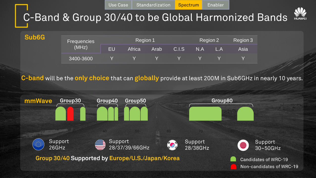
Frequencies
(MHz)
Region 1 Region 2 Region 3
EU Africa Arab C.I.S N.A L.A Asia
3400-3600 Y Y Y Y Y Y Y

15
• 单击此处编辑母版文本样式
– 第二级 • 第三级
– 第四级
» 第五级
2017/1/18 15
•
•
•
•
•
•
•
•
•
•
•
•
•
•
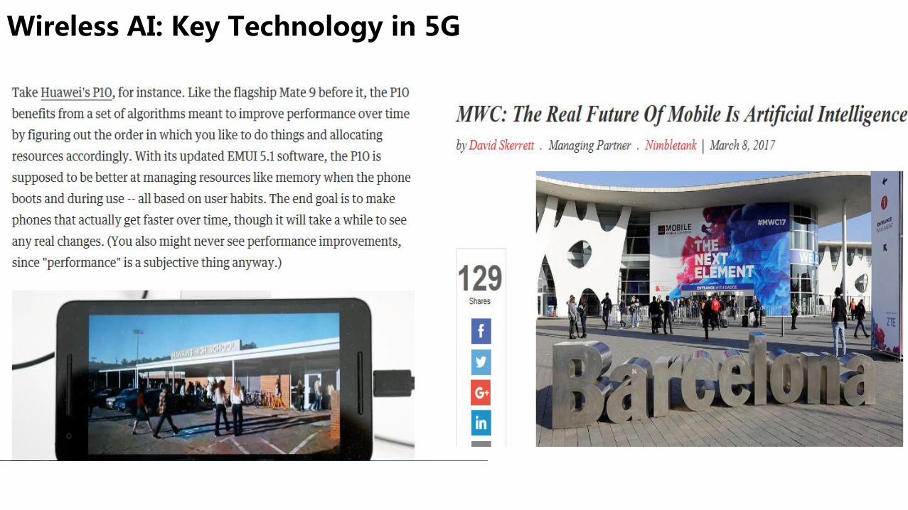
Wireless AI: Key Technology in 5G

HISILICON SEMICONDUCTOR HUAWEI TECHNOLOGIES CO., LTD. Page 15
Wireless AI: Key Technology in 5G AI/ML
ML CV
Robo NLP
Exp. Sys. …
DL
What is Wireless AI
ms
seconds
minutes
hours
days
months
Execution
AI Algorithm Wireless Algorithm
Value Data Link
Scenario Automatically Manually
Target Global probability optimization
Local determined optimization
Scope E2E network Locally Modelling
method Big data, learning Formula , optimization
Usage Set the target goal Tune parameters manually
Big Data
Network
TRM RRM
RTT IRF ANT
NLPS MBB
RNP/O
Chipset
Product
Wireless Alg.
AI in Wireless Network Comparison
RTT
RRM
MBB
OSS
Wireless Brain
Goal oriented and self control in network
management and optimization solution, can
overcome the problem when the network cannot
be accurately expressed with formula based on big
data and machine learning technology.
RB
Feature
Feature Carrier Cell RAT Slice
RTT RRM
OSS/SON
MBB/Core Conf. and Opti.
Policy & Monitor
HUAWEI TECHNOLOGIES CO., LTD.
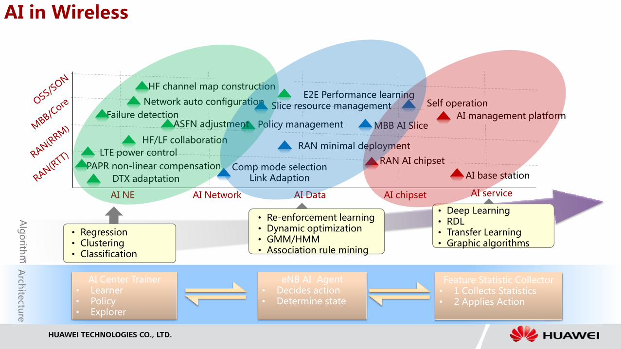
AI in Wireless
AI NE AI Network AI Data AI chipset AI service
AI base station
Network auto configuration
Failure detection Policy management
RAN minimal deployment
RAN AI chipset
DTX adaptation
Self operation
MBB AI Slice
E2E Performance learning
Comp mode selection Link Adaption
PAPR non-linear compensation
• Regression • Clustering • Classification
• Deep Learning • RDL • Transfer Learning • Graphic algorithms
Slice resource management
ASFN adjustment
• Re-enforcement learning • Dynamic optimization • GMM/HMM • Association rule mining
HF/LF collaboration
LTE power control
HF channel map construction
AI management platform
Alg
orith
m
Arch
itectu
re
AI Center Trainer • Learner • Policy • Explorer
eNB AI Agent • Decides action • Determine state
Feature Statistic Collector • 1 Collects Statistics • 2 Applies Action

HISILICON SEMICONDUCTOR HUAWEI TECHNOLOGIES CO., LTD. Page 17
Failure Detection and Analysis
Network Planning and Optimization
More Accurate
More Intelligent
More Faster
Wireless Brain
Network Resource Management
Architecture
Platform
Dataset
AI in wireless network
Physical Sub-health detection VoLTE root cause analysis Failure prediction Network security risk analysis
Traffic prediction Experienced network AI in SON Use behavior analysis
CA policy selection Slice resource management Intelligent base station MEC deployment
AI/ML technique is designed into the network pipe, to
enable wireless network autonomic
Improve the network operations
Reduce the complexity of network fault diagnosis
New deep learning network architecture has
been proposed
Rapid development of unsupervised learning
Development of AI chipset /TPU
Technique trend in AI/ML
Trend when AI/ML used in wireless network
Reconstruct Wireless network using AI technique
Handling mobile video traffic: Solutions and future challenges
Stefan VALENTIN Principal Researcher
Leader of the Context-Aware Optimization Team
Mathematical and Algorithmic Sciences Lab, Paris Research Center, Huawei, France
February 2017

Outline
• Mobile video traffic: Load and main characteristics
• 3 solutions to handle mobile video traffic
– Traffic shaping: T-Mobile and us
– Radio Resource Management: Buffers and radio maps
– Traffic profiling: Real-time traffic analytics by machine learning
• The future:
– QoE-estimation at the edge
– VR and cloud rendering
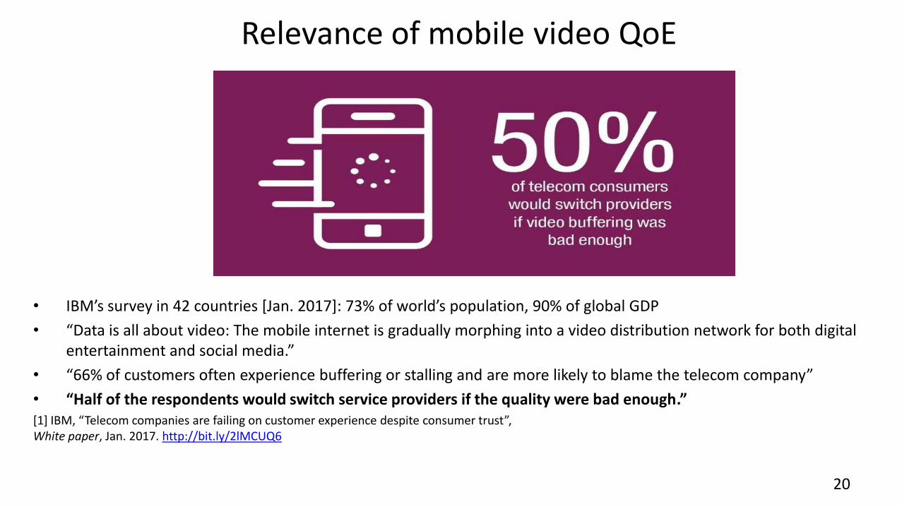
Relevance of mobile video QoE
• IBM’s survey in 42 countries [Jan. 2017]: 73% of world’s population, 90% of global GDP
• “Data is all about video: The mobile internet is gradually morphing into a video distribution network for both digital entertainment and social media.”
• “66% of customers often experience buffering or stalling and are more likely to blame the telecom company”
• “Half of the respondents would switch service providers if the quality were bad enough.” [1] IBM, “Telecom companies are failing on customer experience despite consumer trust”, White paper, Jan. 2017. http://bit.ly/2lMCUQ6
20
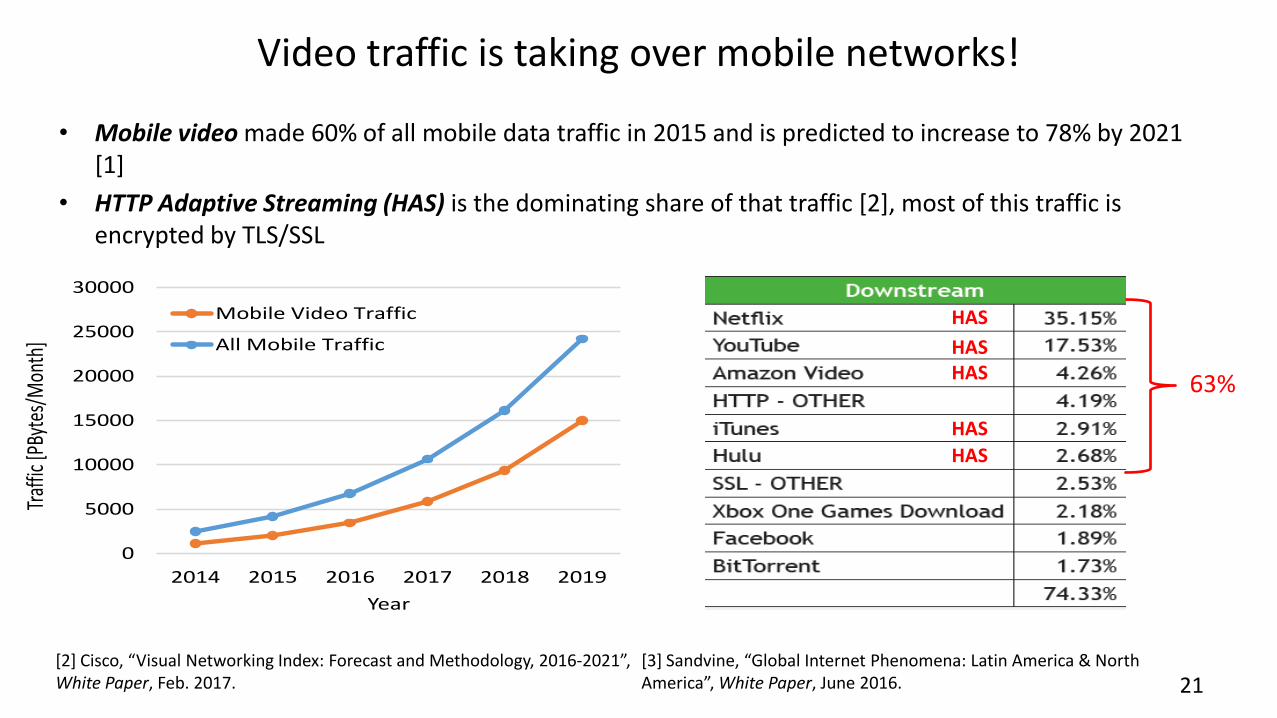
Video traffic is taking over mobile networks!
• Mobile video made 60% of all mobile data traffic in 2015 and is predicted to increase to 78% by 2021 [1]
• HTTP Adaptive Streaming (HAS) is the dominating share of that traffic [2], most of this traffic is encrypted by TLS/SSL
0
5000
10000
15000
20000
25000
30000
2014 2015 2016 2017 2018 2019
Traf
fic [P
Byte
s/M
onth
]
Year
Mobile Video Traffic
All Mobile Traffic
[2] Cisco, “Visual Networking Index: Forecast and Methodology, 2016-2021”, White Paper, Feb. 2017. 21
[3] Sandvine, “Global Internet Phenomena: Latin America & North America”, White Paper, June 2016.
HAS
HAS HAS
HAS
HAS
63%

Outline
• Mobile video traffic: Load and main characteristics
• 3 solutions to handle mobile video traffic
– Traffic shaping: T-Mobile and us
– Radio Resource Management: Buffers and radio maps
– Traffic profiling: Real-time traffic analytics by machine learning
• The future:
– QoE-estimation at the edge
– VR and cloud rendering
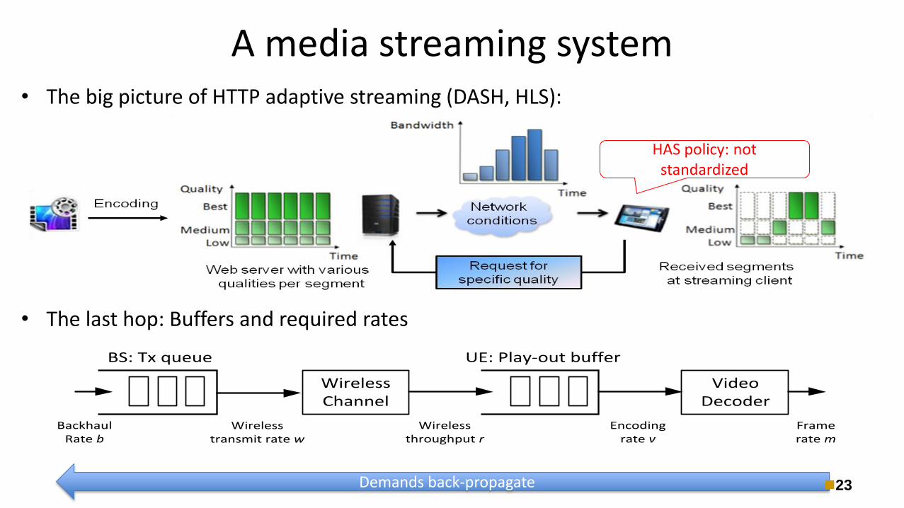
A media streaming system • The big picture of HTTP adaptive streaming (DASH, HLS):
• The last hop: Buffers and required rates
Wireless Channel
Video Decoder
Encoding rate v
Wireless throughput r
Frame rate m
BS: Tx queue UE: Play-out buffer
Wireless transmit rate w
BackhaulRate b
HAS policy: not standardized
Demands back-propagate 23

Adaptive streaming: traffic generation • HAS policy is a load scheduler with 3 main components:
1. Predict throughput for next time slots
2. Select video quality (bitrate) V
3. Schedule download of next segment at V
• A blueprint:
24
[4] Z. Li, X. Zhu, J. Gahm, R. Pan, H. Hu, A. Begen, and D. Oran, “Probe and adapt: rate adaptation for HTTP video streaming at scale,” IEEE JSAC, Apr. 2014
Construction principle for most HAS policies

A closer look on HAS traffic: YouTube
• Since 2013, YouTube: – Consistently uses H.264 in MP4 containers and often offers VP9 in the WebM container – Uses DASH with separate representations for audio and video
• We study: – TCP/IP packet traces of YouTube player application in Android 6.1 on the Motorola Nexus 6 – Big Bucks Bunny (BBB) movie streamed via LTE (Orange, high throughput) – Video: 9m56s duration, high motion, 4 qualities 1080p/4Mbps, 720p/2Mbps, 460p/1Mbps and 360p/0.6Mbps – Only H.264/MP4 version is streamed, encoding rate is extracted with ffprobe
https://www.youtube.com/watch?v=YE7VzlLtp-4
Manifest parser: http://www.h3xed.com/blogmedia/youtube-info.php
25

The 3 phases of a streaming session
• Example of clearly defined buffer/steady state/depleting phases.
Cumulative sum of streaming data over time for Android YouTube App via LTE, 9:56 min BBB movie, constant 480p quality
26

The 3 phases with a DASH quality change
Cumulative sum of streaming data over time for Android YouTube App via LTE, 9:56 min BBB movie , 480p until 3min and then 720p
27

Observations from YouTube traffic
• Further observations: – High dynamic of encoding rate does not show: But GoP structure can be identified from MTU runs – Large GoPs are used for many videos, usually 120-GoP – Client opens a large number of ports (~50) per session but only few are used for streaming – Client uses persistent HTTP: Ports are kept open – Client abandons buffer in case of a quality change
• Two phases with different rate requirements: – Filling phase: High rate required initially, with quality changes and stalls – Steady state: Constant average rate, close to average video encoding rate – Begin of steady state can be detected from observing traffic rate
• Conclusions for wireless scheduler design: – Filling phase requires separate treatment with high priority – Otherwise: Steady state assumption requires CBR (on the average)
28
Outline
• Mobile video traffic: Load and main characteristics
• 3 solutions to handle mobile video traffic
– Traffic shaping: T-Mobile and us
– Radio Resource Management: Buffers and radio maps
– Traffic profiling: Real-time traffic analytics by machine learning
• The future:
– QoE-estimation at the edge
– VR and cloud rendering

T-Mobile USA deployed static rate limitation in Nov. 2015 as part of their Binge On program [12]
Video traffic is identified at the P-Gateway and rate is limited to 1.5 Mbit/s for this traffic [12, 13].
This limit forces HAS players to choose 480p quality, which is medium quality in most services
Business case: Limiting video load allows T-Mobile to offer contracts without data cap at the same capex [12].
Problem 1: Service providers have to provide tags in order to identify the video => Requires cooperation and easy to exploit
Problem 2: Static rate limit increases buffering time. The result is poor QoE due to higher initial playback delay, fast forward time, stalling time etc.
Problem 3: Static limit always penalizes video traffic – bad publicity for T-Mobile [14]. The chosen limit is too low for modern handsets (≥ 1080p displays) and delivers poor QoE for interactive services (e.g., 360°video).
T-Mobile’s problem: RAN flooded by video traffic
30
A/V decoder
HAS policy
Modem
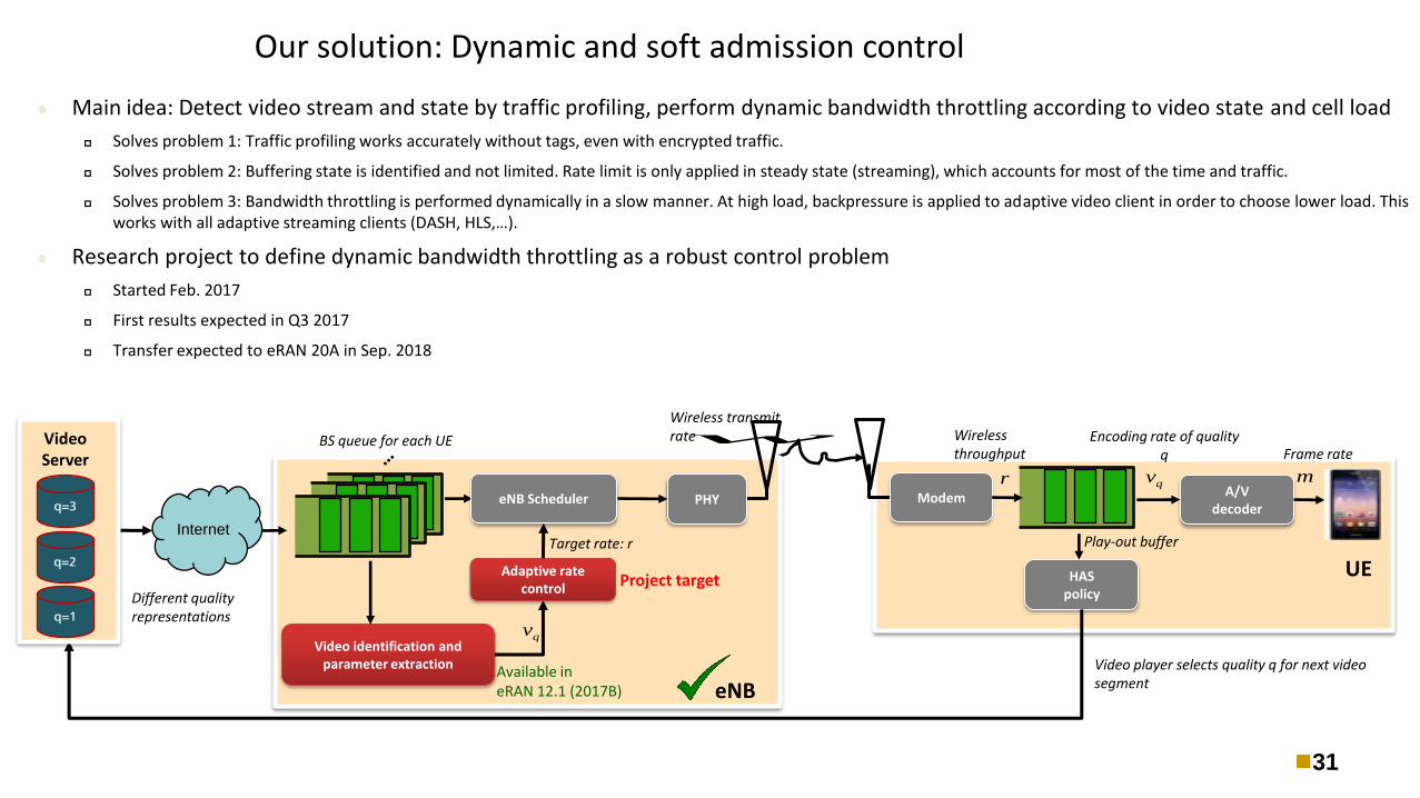
Main idea: Detect video stream and state by traffic profiling, perform dynamic bandwidth throttling according to video state and cell load
Solves problem 1: Traffic profiling works accurately without tags, even with encrypted traffic.
Solves problem 2: Buffering state is identified and not limited. Rate limit is only applied in steady state (streaming), which accounts for most of the time and traffic.
Solves problem 3: Bandwidth throttling is performed dynamically in a slow manner. At high load, backpressure is applied to adaptive video client in order to choose lower load. This works with all adaptive streaming clients (DASH, HLS,…).
Research project to define dynamic bandwidth throttling as a robust control problem
Started Feb. 2017
First results expected in Q3 2017
Transfer expected to eRAN 20A in Sep. 2018
Our solution: Dynamic and soft admission control
Internet
PHY
BS queue for each UE
Video identification and parameter extraction
q=1
Video Server
q=2
q=3
eNB
UE
Play-out buffer
Video player selects quality q for next video segment
Target rate: r
Different quality representations
Wireless transmit rate Encoding rate of quality
q
qv
Wireless throughput
r
Frame rate
m
qv
eNB Scheduler
w
Adaptive rate control
Available in eRAN 12.1 (2017B)
Project target
31

ARRM: Architecture
• Base station or RAN controller: Runs a buffer model to be aware of the user’s buffer state.
Allocates fraction of channel resources to K users over a prediction horizon of T time slots
Predicts wireless channel rate and streaming rate, may identify state changes
32
ĥ
Radio
Maps
CQI
eNB
Long-term channel state prediction (LTCP) Anticipatory scheduler
Short-term channel state prediction (STCP)
Play-out buffer model
Buffer state
Streaming rate estimation (SRE)
Context Information
QCD, SVMs
SVMs
E[ĥ] Allocated PRBs

ARRM: Main idea • Fill playback buffer in advance at high SINR, consume buffer at low SINR => No resources required at poor coverage => Spectral efficiency gain • Toy example for one user moving between 2 cells:
Cell edge
Fill buffer Allocation too costlyConsume buffer
Required bit rate
33
[5] S. Sadr and S. Valentin, “Anticipatory Buffer Control and Resource Allocation for Wireless Video Streaming," arXiv:1304.3056v1, 2013
[6] Z. Lu and G. de Veciana, “Optimizing stored video delivery for mobile networks: The value of knowing the future,“ in Proc. INFOCOM, 2013
Cell edge
Fill buffer Allocation too costlyConsume buffer
Required bit rate

Buffer evolution and stalling time
Improvement over [11]: Feasible solution even when we have stalls
ARRM playback buffer model
34
• Comments: • Buffer limit Z allows to trade off capacity versus buffer size • Large buffer wastes channel capacity if the user drops the video or jumps in it • Time-index in V covers HAS
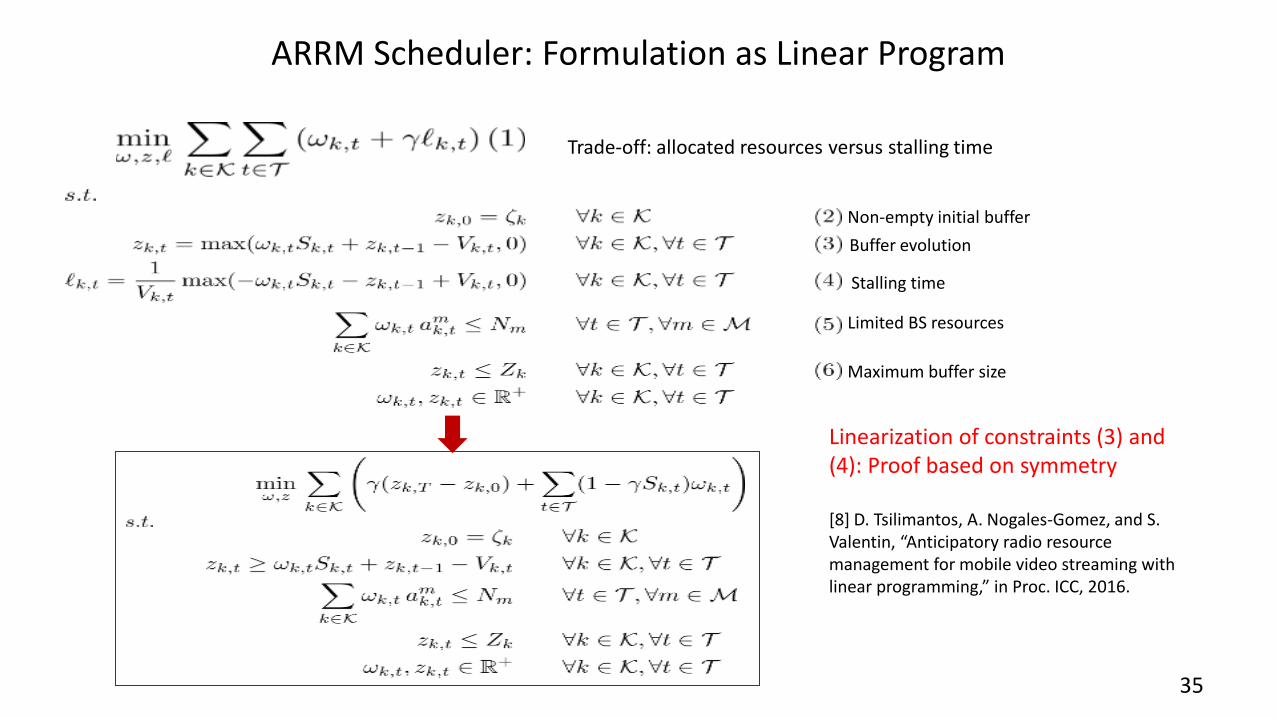
ARRM Scheduler: Formulation as Linear Program
Trade-off: allocated resources versus stalling time
Non-empty initial buffer
Buffer evolution
Stalling time
Limited BS resources
Linearization of constraints (3) and (4): Proof based on symmetry [8] D. Tsilimantos, A. Nogales-Gomez, and S. Valentin, “Anticipatory radio resource management for mobile video streaming with linear programming,” in Proc. ICC, 2016.
Maximum buffer size
35

System Simulation: Parameters [9]
• Proof of concept scenario: Video user move from left to right cell
• Large number of best effort users randomly dropped
36

Exploiting memory by anticipation
• We can expect high spectral efficiency gains by filling the user’s playout buffer in advance
Large buffer: Higher spectral efficiency but a higher risk that user drops the video. More
accurate prediction required.
Small buffer: Require more channel resources to fulfill the minimum bitrate constraint before the buffer runs empty
37
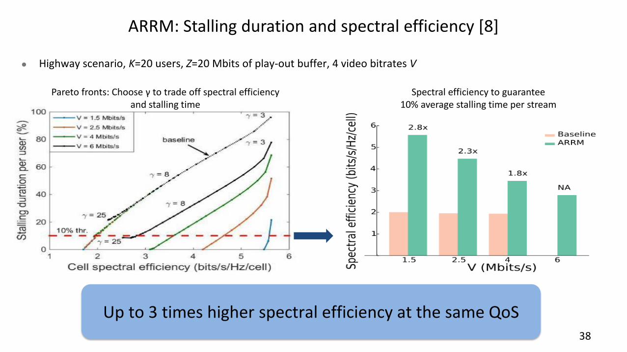
Up to 3 times higher spectral efficiency at the same QoS
ARRM: Stalling duration and spectral efficiency [8]
Highway scenario, K=20 users, Z=20 Mbits of play-out buffer, 4 video bitrates V
Pareto fronts: Choose γ to trade off spectral efficiency and stalling time
Spectral efficiency to guarantee 10% average stalling time per stream
38

ARRM: Stalling probability [8]
Multi-user, highway model, Z = 20 Mbits, 4 video bitrates V
Up to 5 times more users supported at the same QoS
Probability of zero stalls
Number of supported users with guaranteed less than 10% stalling probability
39

Computational time [8]
Empirical cdf of one optimization for ARRM with T = 20 slots
Measured on: Intel Xeon CPU running at 3.3 GHz running CPLEX v12.6 with C interface
40

Current field tests: Scenario
•Traffic configuration •Ue0~Ue5: Video traffic, fixed Rate:1.2Mbps, fixed segment duration:10s •Ue6~Ue9:Background User, file size:625kBytes, file interval:5s
•Scenario 1Cell, 6Video User+ 4Bk User Video User access the network in turns Simulation time :480 seconds RSRP: UE0,UE6:-71.78dB UE1,UE2,UE3,UE7,UE8:-116.78dB UE4,UE5,UE9:-121.78dB
41
Collaboration with Wireless BU, Shanghai
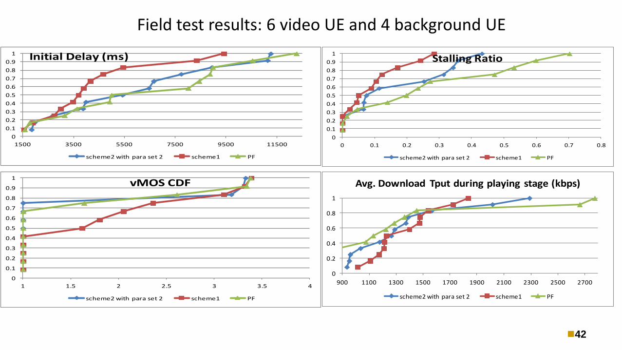
Field test results: 6 video UE and 4 background UE
0
0.1
0.2
0.3
0.4
0.5
0.6
0.7
0.8
0.9
1
1 1.5 2 2.5 3 3.5 4
vMOS CDF
scheme2 with para set 2 scheme1 PF
0
0.1
0.2
0.3
0.4
0.5
0.6
0.7
0.8
0.9
1
0 0.1 0.2 0.3 0.4 0.5 0.6 0.7 0.8
Stalling Ratio
scheme2 with para set 2 scheme1 PF
0
0.1
0.2
0.3
0.4
0.5
0.6
0.7
0.8
0.9
1
1500 3500 5500 7500 9500 11500
Initial Delay (ms)
scheme2 with para set 2 scheme1 PF
0
0.2
0.4
0.6
0.8
1
900 1100 1300 1500 1700 1900 2100 2300 2500 2700
Avg. Download Tput during playing stage (kbps)
scheme2 with para set 2 scheme1 PF
42

ARRM: Architecture
• Base station or RAN controller: Runs a buffer model to be aware of the user’s buffer state.
Allocates fraction of channel resources to K users over a prediction horizon of T time slots
Predicts wireless channel rate and streaming rate, may identify state changes
43
ĥ
E[ĥ] Radio
Maps
Allocated PRBs
CQI
eNB
Long-term channel state prediction (LTCP) Anticipatory scheduler
Short-term channel state prediction (STCP)
Play-out buffer model
Buffer state
Streaming rate estimation (SRE)
Context Information
QCD, SVMs
SVMs

HUAWEI TECHNOLOGIES CO., LTD. Page 44
Matrix Completion for radiomaps

HUAWEI TECHNOLOGIES CO., LTD. Page 45
HUAWEI TECHNOLOGIES CO., LTD. Page 46
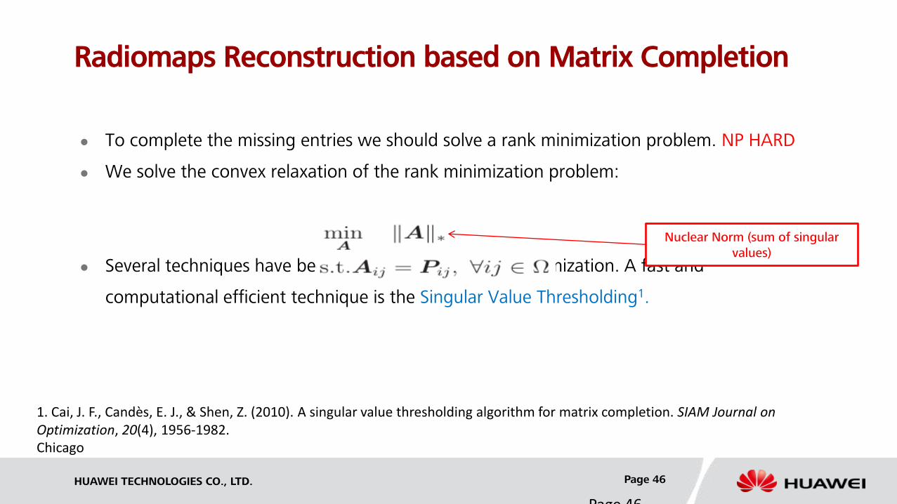
Radiomaps Reconstruction based on Matrix Completion
To complete the missing entries we should solve a rank minimization problem. NP HARD
We solve the convex relaxation of the rank minimization problem:
Several techniques have been proposed to solve this optimization. A fast and
computational efficient technique is the Singular Value Thresholding1.
Page 46
Nuclear Norm (sum of singular
values)
1. Cai, J. F., Candès, E. J., & Shen, Z. (2010). A singular value thresholding algorithm for matrix completion. SIAM Journal on Optimization, 20(4), 1956-1982. Chicago

HUAWEI TECHNOLOGIES CO., LTD. Page 47
Singular Value Thresholding Algorithm
Rank reduction operator

HUAWEI TECHNOLOGIES CO., LTD. Page 48
Improvements over state-of-the-art
non-adaptive reconstruction techniques
Example: Berlin Pathloss map reconstruction:
Size of Area 7500m X 7500m
Size of Pixel 50m
Number of Base Stations: 187
HUAWEI TECHNOLOGIES CO., LTD. Page 49
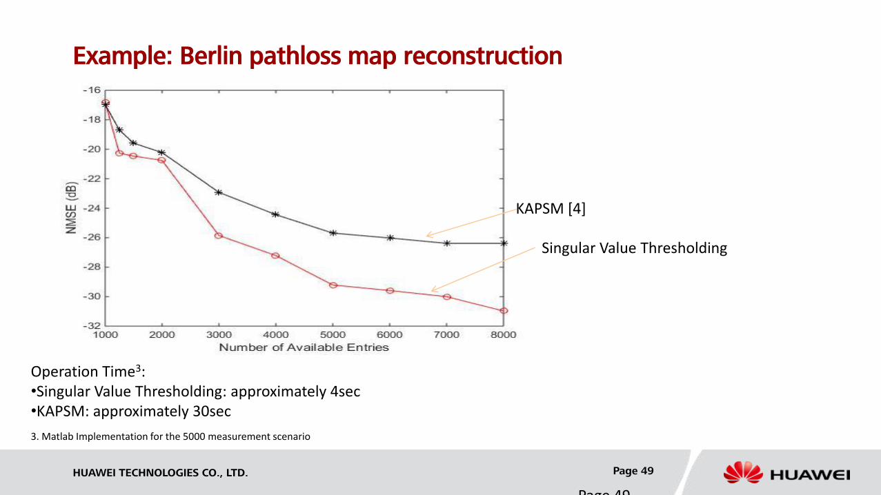
Example: Berlin pathloss map reconstruction
Page 49
KAPSM [4]
Singular Value Thresholding
Operation Time3: •Singular Value Thresholding: approximately 4sec •KAPSM: approximately 30sec 3. Matlab Implementation for the 5000 measurement scenario
HUAWEI TECHNOLOGIES CO., LTD. Page 50
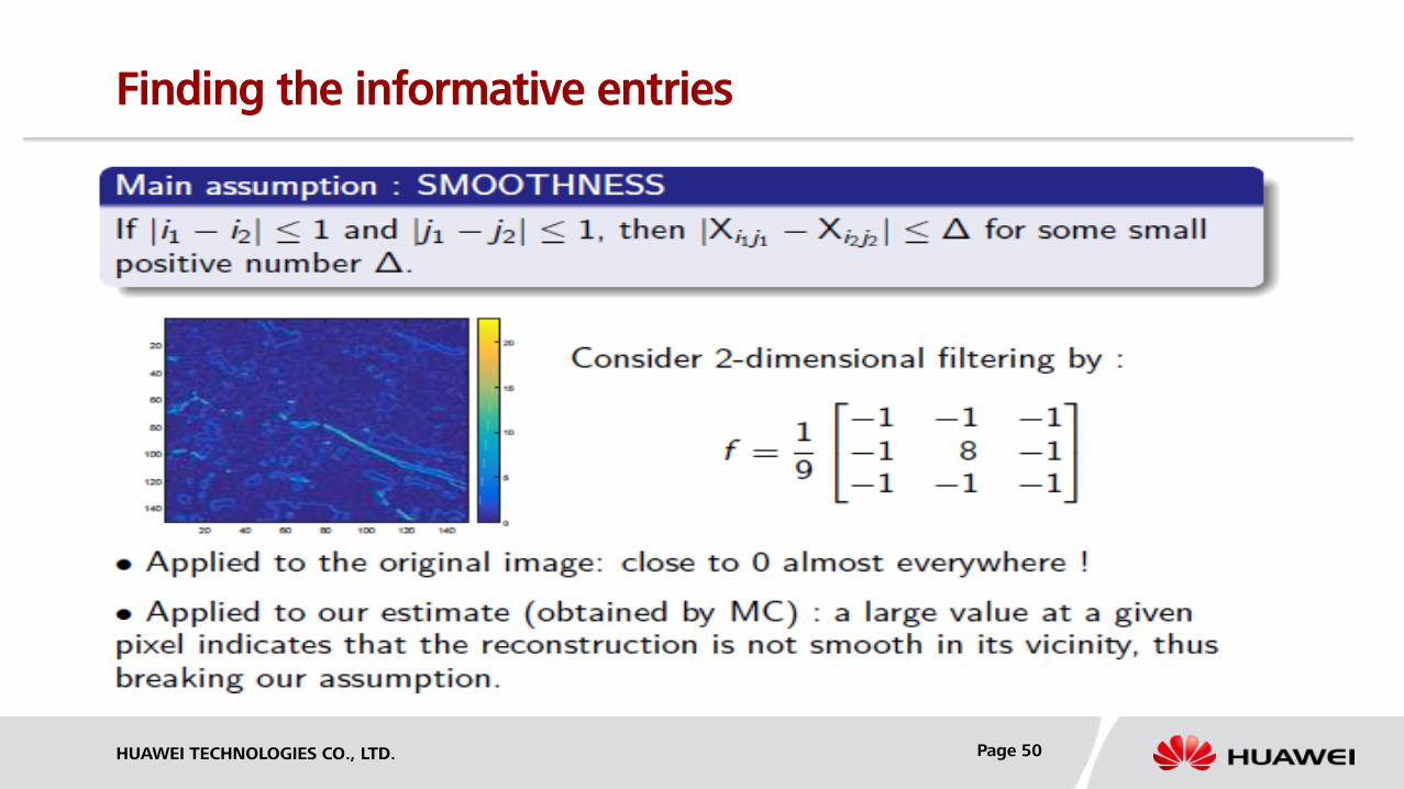
Finding the informative entries

HUAWEI TECHNOLOGIES CO., LTD. Page 51
Finding the informative entries
• URS: Sample the N extra entries at random
• QbC: run different algorithms in parallel and sample the N extra entries that score the largest error
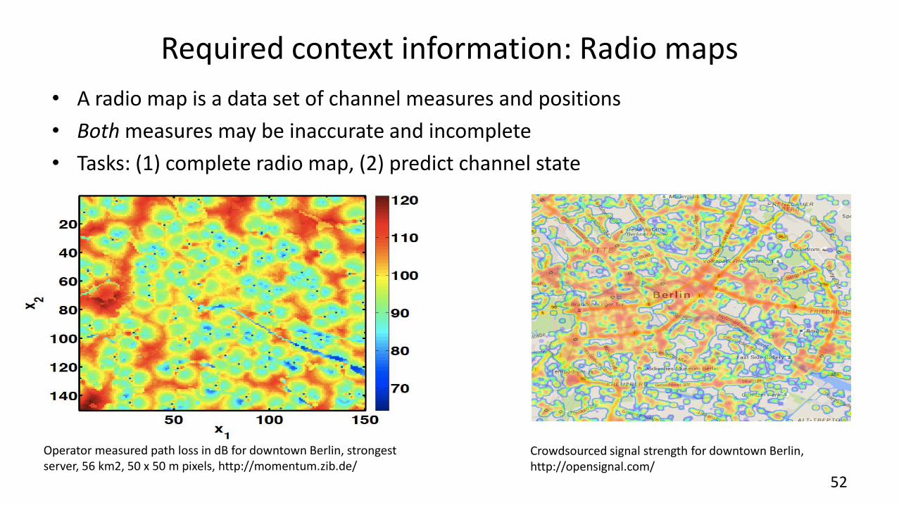
Required context information: Radio maps
• A radio map is a data set of channel measures and positions
• Both measures may be inaccurate and incomplete
• Tasks: (1) complete radio map, (2) predict channel state
Operator measured path loss in dB for downtown Berlin, strongest server, 56 km2, 50 x 50 m pixels, http://momentum.zib.de/
Crowdsourced signal strength for downtown Berlin, http://opensignal.com/
52

Illustration for the Berlin map
Original Pathloss Map Pathloss Map: Missing entries, 40% of the complete data
Reconstructed Pathloss Map
Pathloss map can be approximately reconstructed using a small number of measurements
[7] S. Chouvardas, S. Valentin, M. Draief and M. Leconte, "A Method to Reconstruct Coverage Loss Maps Based on Matrix Completion and Adaptive Sampling", ICASSP, 2016. Submitted to 53

Accuracy for the Berlin map
APSM [8]
Singular Value Thresholding
4.5 dB accuracy gain
Runtime (Matlab for 5000 samples): • Singular Value Thresholding: approximately 4 s • APSM: approximately 30 s
[8] M. Kasparick, R. L. G. Cavalcante, S. Valentin, S. Stanczak, M. Yukawa, "Kernel-Based Adaptive Online Reconstruction of Coverage Maps With Side Information," IEEE TVT, Vol. PP(99), Jul. 2015. 54
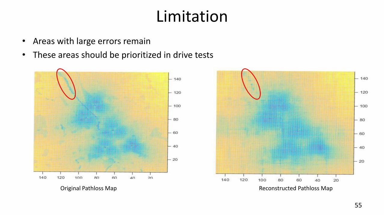
Limitation
• Areas with large errors remain
• These areas should be prioritized in drive tests
Original Pathloss Map Reconstructed Pathloss Map
55

• Users collect the n’th sample at time tn and provide it to a central data base, the sample contains: – Timestamped location:
– Corresponding channel gain:
• Basic model: Linear regression
where base function Φ is expressed by a superposition of Gaussian Kernels
• The hyperparameters of this kernel are found by minimizing the negative log marginal likelihood
Channel prediction with Bayesian spatio-temporal inference
56

Data-based simulation • Scenario: Berlin coverage map of 56 km2 from MOMENTUM project (T-Mobile), street data from
OpenStreetMap
• Vehicular mobility for 100 users generated by SUMO, users leave map
57
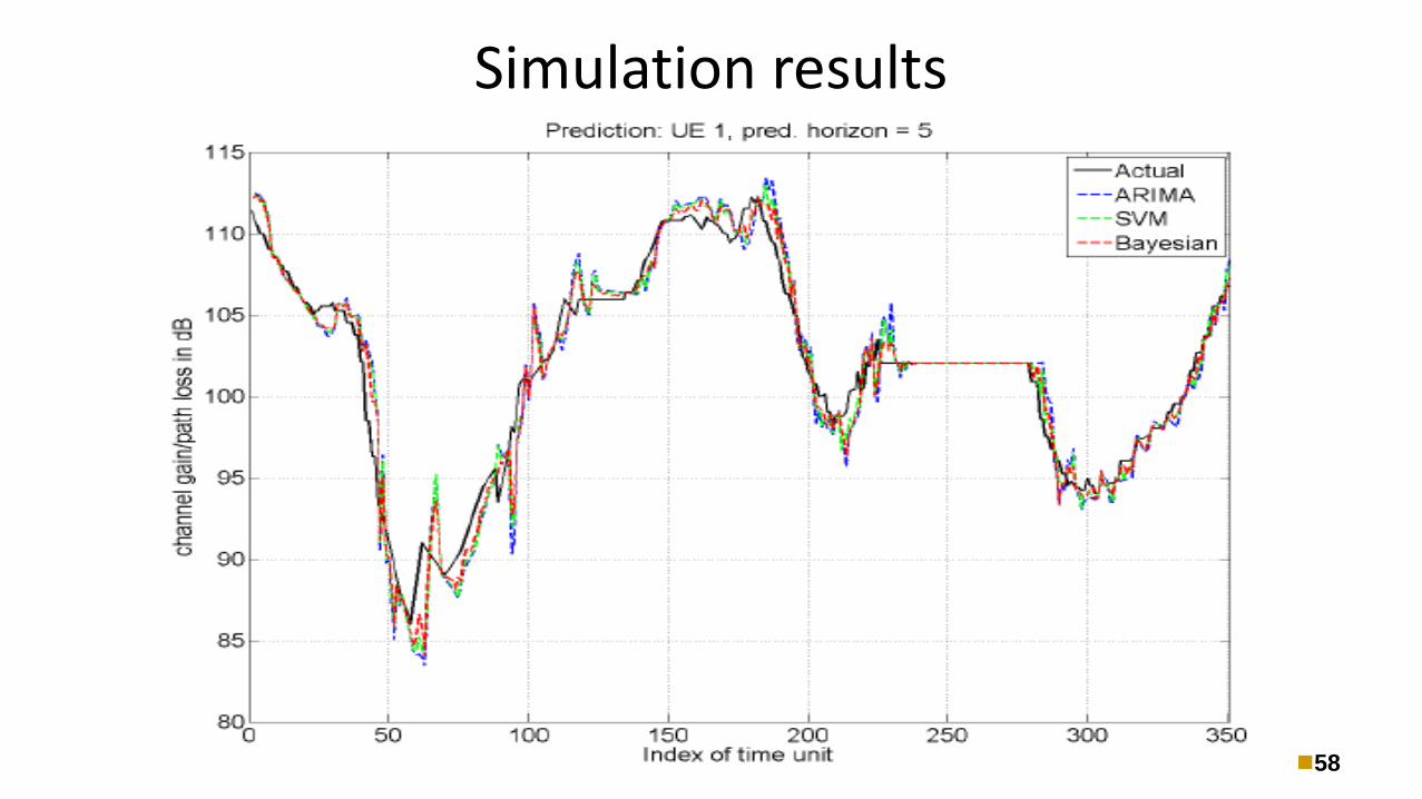
Simulation results
58

Simulation results
59 [9] Q. Liao, S. Valentin, and S. Stanczak, “Channel Gain Prediction in Wireless Networks Based on Spatial-Temporal Correlation”, in Proc. IEEE SPAWC, Jun. 2015.
With 150 m localization error
RM
SE [
dB
]
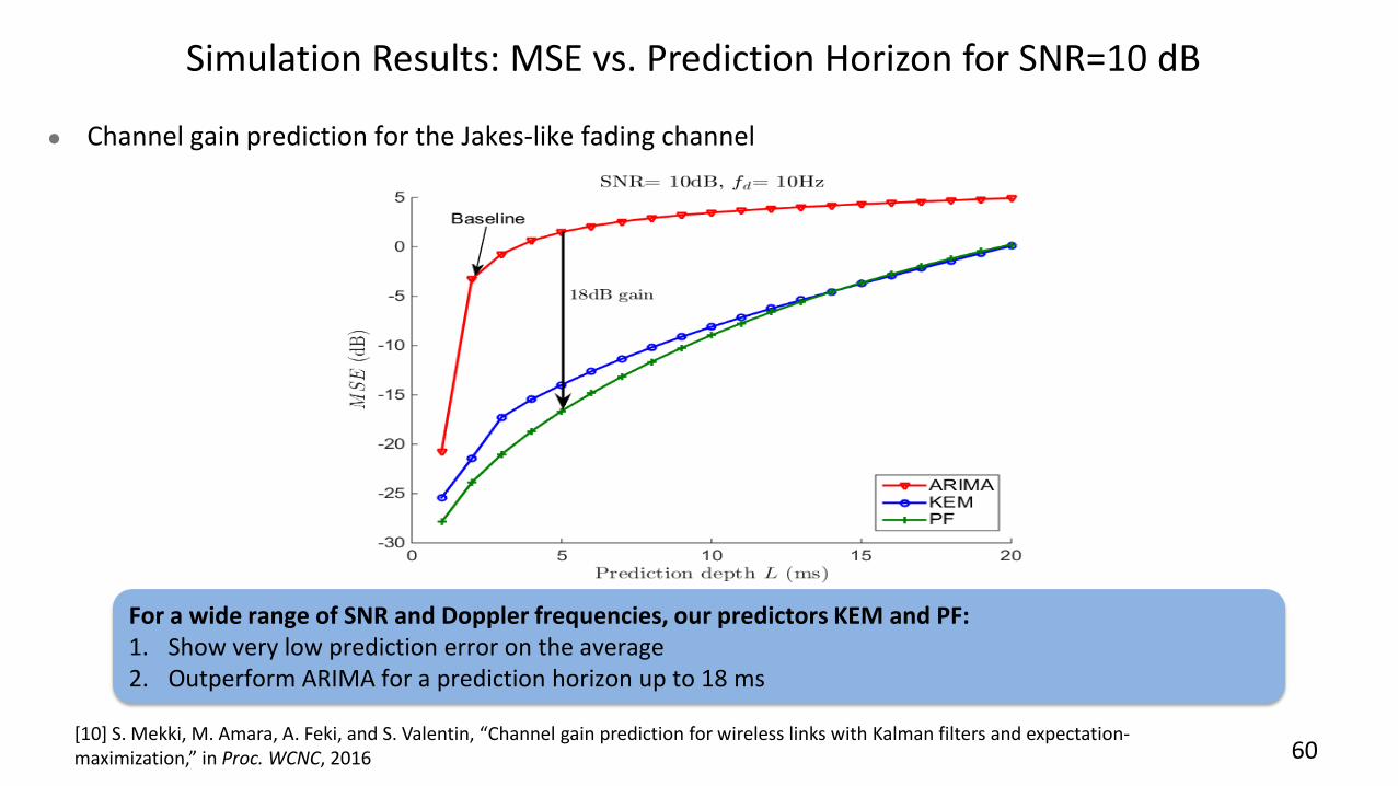
Simulation Results: MSE vs. Prediction Horizon for SNR=10 dB
For a wide range of SNR and Doppler frequencies, our predictors KEM and PF: 1. Show very low prediction error on the average 2. Outperform ARIMA for a prediction horizon up to 18 ms
Channel gain prediction for the Jakes-like fading channel
60 [10] S. Mekki, M. Amara, A. Feki, and S. Valentin, “Channel gain prediction for wireless links with Kalman filters and expectation-maximization,” in Proc. WCNC, 2016
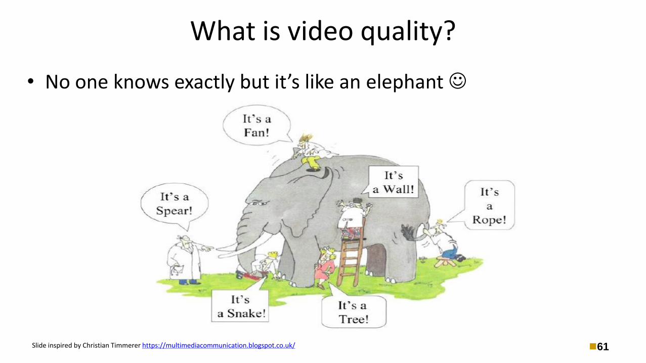
What is video quality?
• No one knows exactly but it’s like an elephant
Slide inspired by Christian Timmerer https://multimediacommunication.blogspot.co.uk/
61

Some methodology
• Subjective, objective or estimated [ITU-T P.800.1]
• Subjective: • MOS (ITU-T P.910): a generally accepted method of subjective measurement. Details are defined by P.910
(ACR,ACR-HR,DCR and PC methods).
• P.NAMS (ITU-T P.1200): the standard of non-intrusive assessment of audiovisual media streaming quality established by ITU-T.
• P.NATS (ITU-T P.1203, Oct. 2016): Parametric bitstream-based quality assessment of progressive download and adaptive audiovisual streaming services over reliable transport
• Objective (QoE factors): • PSNR, playback starting delay, buffering duration, streaming rate, stability [11]
• Estimated: JNDMetrix [12], vMOS, U-vMOS,… AI?!
E2E
E2E
Not necessarily E2E
[11] M. Seufert, et al., “A Survey on Quality of Experience of HTTP Adaptive Streaming," IEEE Communications Surveys & Tutorials, Sep. 2014.
[12] M. H. Brill, J. Lubin, P. Costa and J. Pearson, "Accuracy and cross-calibration of video-quality metrics: new methods from ATIS/T1A1,“ in Proc. Int. Conf. on Image Processing, Sep. 2002. 62
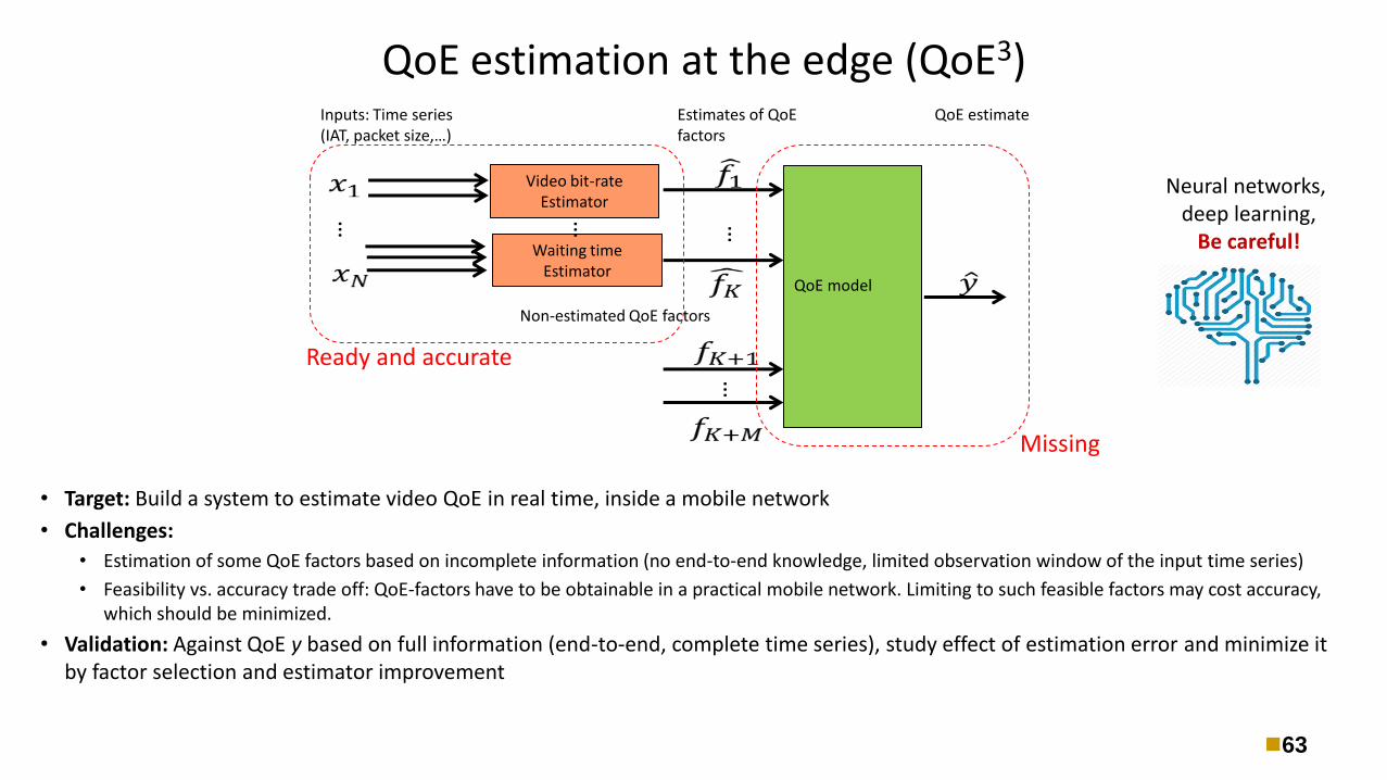
QoE model
QoE estimate
Video bit-rate Estimator
Waiting time Estimator
Estimates of QoE factors
…
…
Inputs: Time series (IAT, packet size,…)
…
Non-estimated QoE factors
…
• Target: Build a system to estimate video QoE in real time, inside a mobile network
• Challenges:
• Estimation of some QoE factors based on incomplete information (no end-to-end knowledge, limited observation window of the input time series)
• Feasibility vs. accuracy trade off: QoE-factors have to be obtainable in a practical mobile network. Limiting to such feasible factors may cost accuracy, which should be minimized.
• Validation: Against QoE y based on full information (end-to-end, complete time series), study effect of estimation error and minimize it by factor selection and estimator improvement
QoE estimation at the edge (QoE3)
Missing
Ready and accurate
Neural networks, deep learning,
Be careful!
63

Thank you www.huawei.com