ascent: adaptive self-configuring sensor … ascent: adaptive self-configuring sensor networks...

1

ASCENT: Adaptive Self-Configuring sEnsor Networks Topologies.

Alberto Cerpa and Deborah Estrin Department of Computer Science, University of California Los Angeles; and

USC/Information Science Institute. {cerpa, destrin}@cs.ucla.edu

February 2001.

Abstract �� ¢ �� ¢��

��

�� ¢ ��

��

�� ¡�� ¢ �� ¢ �� ¢ �� ¡�� ¢��

�� ¢�� ¢��

�� ¢��

�� ¢ �� ¢

�� ¢ ��

�� ¢ ��

�� ¡��

1 Introduction The availability of micro-sensors and low-power wireless communications will enable the deployment of

densely distributed sensor/actuator networks for a wide range of environmental monitoring applications from urban to wilderness environments; indoors and outdoors; and encompassing a variety of data types including acoustic, image, and various chemical and physical properties [24]. The sensor nodes will perform significant signal processing, computation, and network self-configuration to achieve scalable, robust and long-lived networks [1, 7, 8]. More specifically, sensor nodes will do local processing to reduce communications, and consequently, energy costs.

These requirements pose interesting challenges for networking research. One of the challenges arises from the greatly increased level of dynamics. The large number of nodes will introduce increased levels of system dynamics, which in combination with the high level of environmental dynamics will make designing reliable systems a daunting task. Perhaps the most important technical challenge arises from the energy constraints imposed by unattended systems. These systems must be long-lived and operate without manual intervention, which implies that the system itself must execute the measurement and adaptive configuration in an energy constrained fashion. Finally, there are scaling challenges associated with the large numbers of nodes that will co-exist in such networks to achieve desired spatial coverage and robustness.

In this paper, we describe and present experimental performance studies for a form of adaptive self-configuration designed for sensor networks. As we argue in Section 2, such unattended systems will need to self-configure and adapt to a wide variety of environmental dynamics and terrain conditions. These conditions produce regions with non-uniform communication density. We suggest that one of the ways system designers can address such challenging operating conditions is by deploying redundant nodes and designing the system algorithms to make use of that redundancy over time to extend the systems life. In ASCENT, each node assesses

2

its connectivity and adapts its participation in the multi-hop network topology based on the measured operating region. For instance, a node: • Signals when it detects high message loss, requesting additional nodes in the region to join the network in

order to rely messages to it. • Reduces its duty cycle if it detects high message losses due to collisions. • Probes the local communication environment and does not join the multi-hop routing infrastructure until it is

”helpful” to do so. Why can this adaptive configuration not be done from a central node? In addition to the scaling and

robustness limitations of centralized solutions, a single node cannot directly sense the conditions of nodes distributed elsewhere in space. Consequently, other nodes would need to communicate detailed information about the state of their connectivity in order for the central node to determine who should join the multi-hop network. In the absence of energy constraints, one can always achieve a result that is closer to optimal with a central computation. However, when energy is a constraint and the environment is dynamic, distributed approaches are attractive and possibly are the only practical approach [20] because they avoid transmitting dynamic state information repeatedly across the network.

Previous work has presented adaptive distributed MAC and Transport level congestion response [13, 16]. Pottie and Kaiser [20] initiated work in the general area of wireless sensor networks by establishing that scalable wireless sensor networks require multi-hop operation to avoid sending large amounts of data over long distances. They went on to define techniques by which wireless nodes discover their neighbors and acquire synchronism. Given this basic bootstrapping capability, our work addresses the next level of automatic configuration that will be needed to realize envisioned sensor networks, namely, how to form the multi-hop topology [8]. Given the ability to send and receive packets, and the objective of forming an energy-efficient multi-hop network, we apply well-known techniques from MAC layer protocols to the problem of distributed topology formation. Similar techniques have also been applied to multicast transport protocol adjustment of periodic messaging [9].

In the following section we describe a sensor network scenario, stating our assumptions and considerations. Section 3 describes ASCENT in more detail. In Section 4, we present some initial experimental results using ASCENT. Related work is reviewed in Section 5.

2 Distributed Sensor Network Scenario To motivate our research, consider a habitat monitoring sensor network that is to be deployed in a remote

forest. Deployment of this network can be done, for example, by dropping a large number of sensor nodes from a plane, or placing them by hand. In this example, and in many other anticipated applications of ad-hoc wireless sensor networks, the deployed systems must be designed to operate under the following conditions and constraints: • Ad-hoc deployment: we cannot expect the sensor field to be deployed in a regular fashion (e.g. a linear

array, 2-dimensional lattice). More importantly, uniform deployment does not correspond to uniform connectivity owing to unpredictable propagation effects when nodes, and therefore antennae, are close to the ground and other surfaces, such us, obstacles, trees, etc.

• Energy constraints: The nodes (or at least some significant subset) will be untethered for power as well as communications and therefore the system must be designed to expend as little energy as is possible in order to maximize network lifetime.

• Unattended operation under dynamics: the anticipated number of elements in these systems will preclude manual configuration, and the environmental dynamics will preclude design-time pre-configuration.

In many such contexts it will be far easier to deploy larger numbers of nodes initially than to deploy

additional nodes or additional energy reserves at a later date (similar to the economics of stringing cable for wired networks). In this paper we present one way in which nodes can exploit the resulting redundancy in order to extend system lifetime.

3

If we deploy too few nodes, the distance between neighboring nodes will be too great and the packet loss rate will increase; or the energy required to transmit the data over the longer distances will be prohibitive. If we use all deployed nodes simultaneously, the system will be expending unnecessary energy, at best, and at worst the nodes may interfere with one another by congesting the channel. In the process of finding an equilibrium, we are not trying to use a distributed localized algorithm to identify a single unique optimal solution. Rather this form of adaptive self-configuration using localized algorithms is well suited to problems spaces that have a large number of possible solutions. Our experimental results confirm that this is the case for our application.

In the next section, we describe a detailed algorithm for achieving our task. First we enumerate the following assumptions that apply to the remainder of our work since only a single implementation is studied and we do not have the flexibility afforded by a simulation. • We assume a CSMA MAC protocol. This clearly introduces the possibilities for resource contention when

too many neighboring nodes participate in the multihop network. Our basic approach should be relevant to TDMA MACs because distributed slot allocation schemes will also have degraded performance with increased load.

• Our algorithm reacts when links experience high packet loss. We do not detect or repair complete network partitions. We do not deal with network partitions because we address systems whose node density would preclude nodes from being completely isolated from one another. When node density is low, our approach is not needed because in general all nodes will be needed to form an effective network. Of course network partitions can occur in dense arrays when a swath of nodes are destroyed or obstructed. When such network partitions do occur, we believe that complementary system mechanisms will be most useful. For example, exploiting special resources such as long range radios deployed on a subset of deployed nodes, and used sparingly because of the power required. We leave such complementary techniques for network partition detection and repair to future work.

• ASCENT is not a routing or data dissemination protocol. ASCENT simply decides which nodes should join the routing infrastructure. Ad-hoc routing, Data Diffusion, or some other data dissemination mechanism, then runs over this multihop topology. In this respect, routing protocols are complementary to ASCENT.

The following section describes the ASCENT protocol in detail.

3 ASCENT ASCENT consists of several phases. When a node first initializes, it enters into a listening-only phase called

neighbor discovery phase, where each node obtains an estimate of the number of neighbors actively transmitting messages based on local measurements. Upon completion of this phase, nodes enter into the join decision phase, where they decide whether to join the multi-hop diffusion sensor network. During this phase, a node may temporarily join the network for a certain period of time to test whether it contributes to improved connectivity. If a node decides to join the network for a longer time, it enters into an active phase and starts sending routing control and data messages. If a node decides not to join the network, it enters into the adaptive phase, where it turns itself off for a period of time, or reduces its transmission range.

In this section, we describe these phases and their components. Several design choices present themselves in the context of ASCENT. We elaborate on these design choices while we describe the design it. Our initial experiments (Section 4) focus only on a subset of these design choices.

3.1 Introduction

Consider a simple sensor network for data gathering similar to the network described in Section 2. We cannot expect the sensor field to have uniform connectivity due to unpredictable propagation effects in the environment. Therefore, we would expect to find regions with low and high density. As we pointed out in Section 2, ASCENT does not deal with complete network partitions; we assume that there is a high enough node density to connect the entire region. Figure 1 shows a simplified schematic for ASCENT during initialization in

4

a high-density region. For the sake of clarity, we are showing only the formation of a two-hop network. This analysis may be extended to networks of larger sizes.

Initially, only some nodes join the multi-hop network. The other nodes remain passively listening to the messages but not transmitting. This situation is depicted in Figure 1(a). The source starts transmitting data messages toward the sink. Because the sink is at the limit of radio range, it gets very high message loss from the source. The notion of what constitutes high is application dependent, and in our scheme, this is a parameter tunable by the application. We call this situation a communication hole, i.e. the receiver gets high message loss due to poor connectivity with the sender. The sink then starts sending help messages to signal neighbors that are in listen-only mode –also called passive neighbors– to join the network. It is called a help message because its goal is to ask for help to solve a communication problem due to lack of connectivity, i.e. help to repair a communication hole.

Figure 1. Simplified schematic of a self-configurable sensor network.

When a neighbor receives a help message, it may decide to join the network. This situation is illustrated in Figure 1(b). When a node joins the network it starts transmitting and receiving messages, i.e. it becomes an active neighbor. As soon as a node decides to join the network, it signals other passive neighbors of the existence of a new active neighbor by sending a neighbor announcement message. This situation continues until the number of passive nodes that become active stabilizes on a certain value and the cycle stops. When the process completes, the group of newly active neighbors that have joined the network make the delivery of data from source to sink more reliable. The process will re-start when some future network event (e.g. node failure) or environmental effect (e.g. new obstacle) causes message loss again.

Table 1 shows the list of attributes necessary for data messages, and Table 2 shows the message types used by ASCENT. In the next section we highlight some of the more interesting issues that arose in this design.

Table 1. Attributes required by the self-configuration framework in data messages.

1 Elson and Estrin [6] have presented some related work with transaction identifiers that could be used in our scheme.

Data Attributes Motivation

Sequence number A unitary and monotonically increasing sequence number that helps to determine the message loss.

Neighbor identification Included by the sender, it helps the receiver to identify messages from different neighbors. No need for global unique identifier1.

Help flag Sender requests other nodes to join the network. Neighbor Announcement flag Sender indicates it has just joined the network.

Sink Source

Neighbor

Announcements

Active Neighbor

Data Message

Help Messages

Sink Source

Passive

Data Message

Sink Source

(b) Self-configuration transition (a) Communication Hole (c) Final State

5

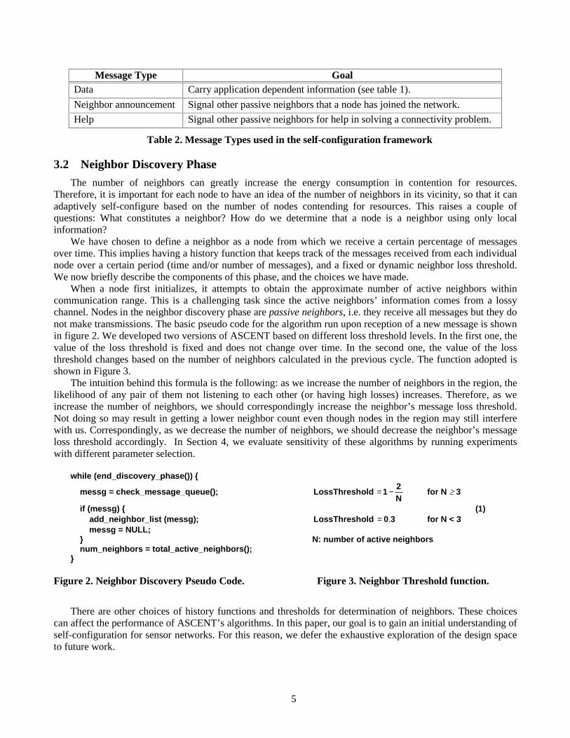
Table 2. Message Types used in the self-configuration framework

3.2 Neighbor Discovery Phase

The number of neighbors can greatly increase the energy consumption in contention for resources. Therefore, it is important for each node to have an idea of the number of neighbors in its vicinity, so that it can adaptively self-configure based on the number of nodes contending for resources. This raises a couple of questions: What constitutes a neighbor? How do we determine that a node is a neighbor using only local information?

We have chosen to define a neighbor as a node from which we receive a certain percentage of messages over time. This implies having a history function that keeps track of the messages received from each individual node over a certain period (time and/or number of messages), and a fixed or dynamic neighbor loss threshold. We now briefly describe the components of this phase, and the choices we have made.

When a node first initializes, it attempts to obtain the approximate number of active neighbors within communication range. This is a challenging task since the active neighbors’ information comes from a lossy channel. Nodes in the neighbor discovery phase are passive neighbors, i.e. they receive all messages but they do not make transmissions. The basic pseudo code for the algorithm run upon reception of a new message is shown in figure 2. We developed two versions of ASCENT based on different loss threshold levels. In the first one, the value of the loss threshold is fixed and does not change over time. In the second one, the value of the loss threshold changes based on the number of neighbors calculated in the previous cycle. The function adopted is shown in Figure 3.

The intuition behind this formula is the following: as we increase the number of neighbors in the region, the likelihood of any pair of them not listening to each other (or having high losses) increases. Therefore, as we increase the number of neighbors, we should correspondingly increase the neighbor’s message loss threshold. Not doing so may result in getting a lower neighbor count even though nodes in the region may still interfere with us. Correspondingly, as we decrease the number of neighbors, we should decrease the neighbor’s message loss threshold accordingly. In Section 4, we evaluate sensitivity of these algorithms by running experiments with different parameter selection.

while (end_discovery_phase()) {

messg = check_message_queue(); N2

1oldLossThresh −= for N t 3

if (messg) { (1) add_neighbor_list (messg); 30oldLossThresh .= for N < 3 messg = NULL; } N: number of active neighbors num_neighbors = total_active_neighbors(); }

Figure 2. Neighbor Discovery Pseudo Code. Figure 3. Neighbor Threshold function.

There are other choices of history functions and thresholds for determination of neighbors. These choices

can affect the performance of ASCENT’s algorithms. In this paper, our goal is to gain an initial understanding of self-configuration for sensor networks. For this reason, we defer the exhaustive exploration of the design space to future work.

Message Type Goal

Data Carry application dependent information (see table 1).

Neighbor announcement Signal other passive neighbors that a node has joined the network.

Help Signal other passive neighbors for help in solving a connectivity problem.

6

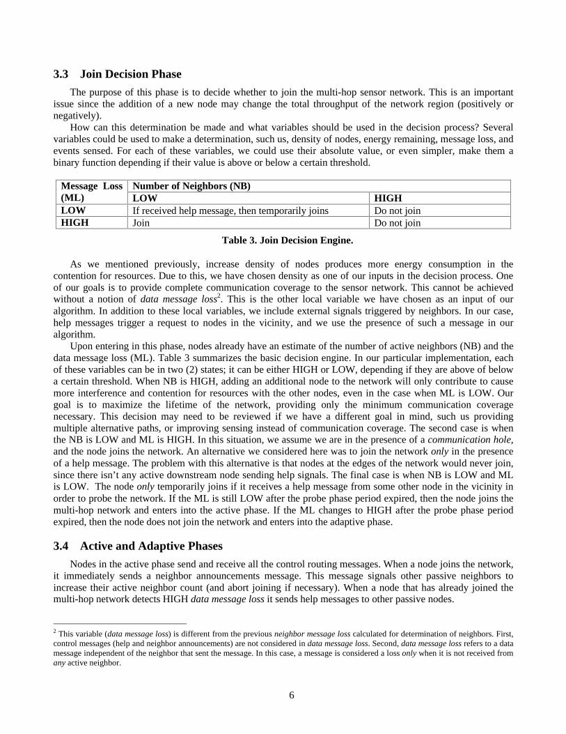
3.3 Join Decision Phase

The purpose of this phase is to decide whether to join the multi-hop sensor network. This is an important issue since the addition of a new node may change the total throughput of the network region (positively or negatively).

How can this determination be made and what variables should be used in the decision process? Several variables could be used to make a determination, such us, density of nodes, energy remaining, message loss, and events sensed. For each of these variables, we could use their absolute value, or even simpler, make them a binary function depending if their value is above or below a certain threshold.

Number of Neighbors (NB) Message Loss

(ML) LOW HIGH LOW If received help message, then temporarily joins Do not join HIGH Join Do not join

Table 3. Join Decision Engine.

As we mentioned previously, increase density of nodes produces more energy consumption in the contention for resources. Due to this, we have chosen density as one of our inputs in the decision process. One of our goals is to provide complete communication coverage to the sensor network. This cannot be achieved without a notion of data message loss2. This is the other local variable we have chosen as an input of our algorithm. In addition to these local variables, we include external signals triggered by neighbors. In our case, help messages trigger a request to nodes in the vicinity, and we use the presence of such a message in our algorithm.

Upon entering in this phase, nodes already have an estimate of the number of active neighbors (NB) and the data message loss (ML). Table 3 summarizes the basic decision engine. In our particular implementation, each of these variables can be in two (2) states; it can be either HIGH or LOW, depending if they are above of below a certain threshold. When NB is HIGH, adding an additional node to the network will only contribute to cause more interference and contention for resources with the other nodes, even in the case when ML is LOW. Our goal is to maximize the lifetime of the network, providing only the minimum communication coverage necessary. This decision may need to be reviewed if we have a different goal in mind, such us providing multiple alternative paths, or improving sensing instead of communication coverage. The second case is when the NB is LOW and ML is HIGH. In this situation, we assume we are in the presence of a communication hole, and the node joins the network. An alternative we considered here was to join the network only in the presence of a help message. The problem with this alternative is that nodes at the edges of the network would never join, since there isn’t any active downstream node sending help signals. The final case is when NB is LOW and ML is LOW. The node only temporarily joins if it receives a help message from some other node in the vicinity in order to probe the network. If the ML is still LOW after the probe phase period expired, then the node joins the multi-hop network and enters into the active phase. If the ML changes to HIGH after the probe phase period expired, then the node does not join the network and enters into the adaptive phase.

3.4 Active and Adaptive Phases

Nodes in the active phase send and receive all the control routing messages. When a node joins the network, it immediately sends a neighbor announcements message. This message signals other passive neighbors to increase their active neighbor count (and abort joining if necessary). When a node that has already joined the multi-hop network detects HIGH data message loss it sends help messages to other passive nodes.

2 This variable (data message loss) is different from the previous neighbor message loss calculated for determination of neighbors. First, control messages (help and neighbor announcements) are not considered in data message loss. Second, data message loss refers to a data message independent of the neighbor that sent the message. In this case, a message is considered a loss only when it is not received from any active neighbor.

7

If a node decides not to join the network, then the question is: what does it do? The answer to this question depends on the problem the sensor network is trying to solve. Nodes could turn themselves off for a certain period of time in order to save energy and extend the network lifetime. They could also reduce their radio range to reduce communication interference while maximizing sensing coverage. Since the goal of our original implementation was to maximize communication coverage and lifetime of the network, we picked the first form of adaptation for our experiments.

We emphasize that, even though we have discussed ASCENT’s algorithms in some detail, much experimentation and evaluation of the various mechanisms and design choices is necessary before we fully understand the robustness, scale and performance of self-configuration. In particular, it is important to test our assumptions with real field experiments, since the level of dynamics we find in the real world is difficult to be captured completely in a simulator. The following section takes an initial step in this direction.

4 Experimental Results In this section, we report results from preliminary performance evaluation of ASCENT. We describe the

experimental testbed used, our methodology, compare the performance of different variations of ASCENT’s algorithms with a static version, and explore the impact of network dynamics and design parameters on our scheme.

4.1 Experimental Testbed

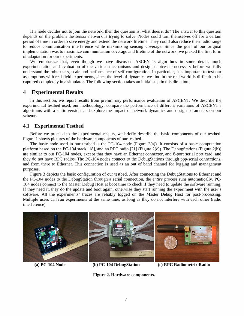
Before we proceed to the experimental results, we briefly describe the basic components of our testbed. Figure 1 shows pictures of the hardware components of our testbed.

The basic node used in our testbed is the PC-104 node (Figure 2(a)). It consists of a basic computation platform based on the PC-104 stack [18], and an RPC radio [21] (Figure 2(c)). The DebugStations (Figure 2(b)) are similar to our PC-104 nodes, except that they have an Ethernet connector, and 8-port serial port card, and they do not have RPC radios. The PC-104 nodes connect to the DebugStations through ppp-serial connections, and from there to Ethernet. This connection is used as an out of band channel for logging and management purposes.

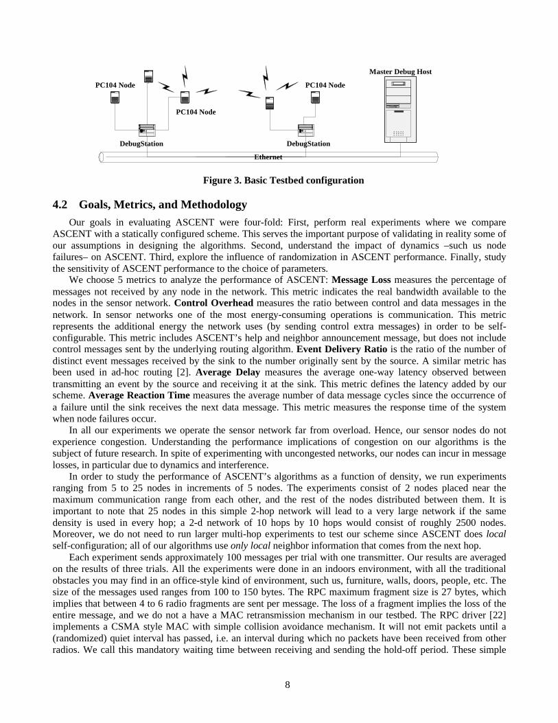
Figure 3 depicts the basic configuration of our testbed. After connecting the DebugStations to Ethernet and the PC-104 nodes to the DebugStation through a serial connection, the entire process runs automatically. PC-104 nodes connect to the Master Debug Host at boot time to check if they need to update the software running. If they need it, they do the update and boot again, otherwise they start running the experiment with the user’s software. All the experiments’ traces are reliably logged on the Master Debug Host for post-processing. Multiple users can run experiments at the same time, as long as they do not interfere with each other (radio interference).

(a) PC-104 Node (b) PC-104 DebugStation (c) RPC Radiometrix Radio

Figure 2. Hardware components.

8

Ethernet

Master Debug Host

DebugStation DebugStation

PC104 Node

PC104 Node

PC104 Node

Figure 3. Basic Testbed configuration

4.2 Goals, Metrics, and Methodology

Our goals in evaluating ASCENT were four-fold: First, perform real experiments where we compare ASCENT with a statically configured scheme. This serves the important purpose of validating in reality some of our assumptions in designing the algorithms. Second, understand the impact of dynamics –such us node failures– on ASCENT. Third, explore the influence of randomization in ASCENT performance. Finally, study the sensitivity of ASCENT performance to the choice of parameters.

We choose 5 metrics to analyze the performance of ASCENT: Message Loss measures the percentage of messages not received by any node in the network. This metric indicates the real bandwidth available to the nodes in the sensor network. Control Overhead measures the ratio between control and data messages in the network. In sensor networks one of the most energy-consuming operations is communication. This metric represents the additional energy the network uses (by sending control extra messages) in order to be self-configurable. This metric includes ASCENT’s help and neighbor announcement message, but does not include control messages sent by the underlying routing algorithm. Event Delivery Ratio is the ratio of the number of distinct event messages received by the sink to the number originally sent by the source. A similar metric has been used in ad-hoc routing [2]. Average Delay measures the average one-way latency observed between transmitting an event by the source and receiving it at the sink. This metric defines the latency added by our scheme. Average Reaction Time measures the average number of data message cycles since the occurrence of a failure until the sink receives the next data message. This metric measures the response time of the system when node failures occur.

In all our experiments we operate the sensor network far from overload. Hence, our sensor nodes do not experience congestion. Understanding the performance implications of congestion on our algorithms is the subject of future research. In spite of experimenting with uncongested networks, our nodes can incur in message losses, in particular due to dynamics and interference.

In order to study the performance of ASCENT’s algorithms as a function of density, we run experiments ranging from 5 to 25 nodes in increments of 5 nodes. The experiments consist of 2 nodes placed near the maximum communication range from each other, and the rest of the nodes distributed between them. It is important to note that 25 nodes in this simple 2-hop network will lead to a very large network if the same density is used in every hop; a 2-d network of 10 hops by 10 hops would consist of roughly 2500 nodes. Moreover, we do not need to run larger multi-hop experiments to test our scheme since ASCENT does local self-configuration; all of our algorithms use only local neighbor information that comes from the next hop.

Each experiment sends approximately 100 messages per trial with one transmitter. Our results are averaged on the results of three trials. All the experiments were done in an indoors environment, with all the traditional obstacles you may find in an office-style kind of environment, such us, furniture, walls, doors, people, etc. The size of the messages used ranges from 100 to 150 bytes. The RPC maximum fragment size is 27 bytes, which implies that between 4 to 6 radio fragments are sent per message. The loss of a fragment implies the loss of the entire message, and we do not a have a MAC retransmission mechanism in our testbed. The RPC driver [22] implements a CSMA style MAC with simple collision avoidance mechanism. It will not emit packets until a (randomized) quiet interval has passed, i.e. an interval during which no packets have been received from other radios. We call this mandatory waiting time between receiving and sending the hold-off period. These simple

9

scheme works because packet arrivals are usually correlated due to fragmentation. Multiple stations that are waiting to transmit will hopefully not collide due to the randomization of the hold-off period. In our experiments, the hold-off period was set to 100 ms and the randomization time to 200 ms. We set these values by carefully measuring the minimum time required by the RPC hardware and driver to transmit consecutive fragments. ASCENT also provides an application level randomization that is set to a maximum of 10 seconds. The data rate is set to 3 messages/min in most of the experiments. We use an implementation of data diffusion [12] as our routing protocol. Underlying routing messages were generated every minute, and the routing timeout was 3 min.

4.3 Comparative Experiments

Our first experiments compare different ASCENT’s algorithms with a static case. We run these experiments when the network initializes, having all the nodes turning on at roughly the same time. This represents the worst-case scenario for our algorithms; nodes base their actions on the number of messages received and multiple nodes may be synchronized to perform the same action at roughly the same time. The likelihood of collisions increases, and correspondingly, the throughput of the network diminishes. The situation would improve if we made the nodes initialize randomly at different times.

Figure 4(a) shows the message loss as a function of the density during initialization. In the static case, all the nodes join the multi-hop network and transmit messages. This algorithm has high message loss because as we increase the density of nodes, the probability of collisions increases accordingly. It rapidly reaches around 80% losses with 15 nodes, and it enters into a saturation region after that. We show here 3 versions of the algorithm presented in Section 3. ASCENT with different fix threshold set the message loss threshold for neighbor determination to 50% (Loss 50) and 80% (Loss 80) respectively. ASCENT’s dynamic algorithm set the threshold dynamically based on the number of neighbor’s value obtained in the previous cycle (Section 3.2). Loss 80 and Dynamic slightly outperform Loss 50, and the three of them significantly outperform the static case. The one transmitter-only curve is included for illustrative purposes. It gives us an idea of the magnitude of the background losses, i.e. losses not due to collisions but due to the environment3.

0

20

40

60

80

100

5 10 15 20 25

Message L

oss (

%)

Number of Nodes

Message Loss vs. Density of Nodes(data rate: 20 sec/msg, win size: 20 msgs)

Static ConfigASCENT DynamicASCENT Loss 80ASCENT Loss 50One transmitter

0

20

40

60

80

100

5 10 15 20 25

Events

deliv

ere

d (

%)

Number of Nodes

Event Delivery Ratio vs. Density of Nodes(data rate: 20 sec/msg, win size: 20 msgs)

Static ConfigASCENT DynamicASCENT Loss 80

0

5

10

15

20

5 10 15 20 25

Contr

ol/D

ata

messages (

%)

Number of Nodes

Control Message Overhead (initialization) vs. Density of Nodes(data rate: 20 sec/msg, win size: 20 msgs)

Static ConfigASCENT DynamicASCENT Loss 80ASCENT Loss 50

(a) Message loss vs. density (b) Delivery Ratio vs. density (c) Control Overhead vs. Density

Figure 4 – Network initialization

Figure 4(b) shows the event delivery ratio, i.e. the percentage of messages transmitted by the source that

reached the sink. Both Loss 80 and Dynamic outperform the static case. Their performance slowly degrades as the density increases, which demonstrates the scalability properties of our algorithms as the number of nodes increases. The static case does not perform as badly as one would expect based on the message loss shown in the previous graph. This is because the event delivery ratio metric measures if at least one copy of the original

3 This curve is not flat, as one would expect beforehand, due to an artifact of our implementation. Our routing algorithm was running all the time, even in the case of passive neighbors. This implies that we do get some losses due to collisions with control routing messages.

10

message sent by the source reaches the sink. Even in a high-density environment with high losses, the likelihood of receiving any copy of the same message from any neighbor is still high. As we increase the network size and enter high-density regions the situation would deteriorate rapidly.

Figure 4(c) shows the control overhead due to the transmission of extra messages. These messages impose an extra energy consumption on the nodes that would not be there if the nodes were not self-configurable. The graph shows that as we increase the density of nodes, the overhead slightly increases. The probability of two nodes in the density region not listening to each other increases as the region gets more densely populated. This causes more nodes to temporarily join the network to probe it, since the individual neighbor counts may not reflect the actual connectivity in all the cases. Therefore, the number of control messages sent increases as the density increases. Having a low loss threshold for neighbor determination makes the system more reactive but at the expense of increase control overhead, which effectively increases the probability of collisions. The graph shows that this overhead is always small, being in the worst-case scenario of 25 nodes below 13%, 9%, and 7% for the Loss 50, Loss 80 and Dynamic cases respectively.

4.4 Impact of Dynamics

To study the impact of dynamics on ASCENT, we turn off one or more active nodes while in the steady state regime (after initialization). This helps us to measure how ASCENT reacts in the presence of one or multiple node failures. We hoped that our algorithms would have overhead linear to the number of nodes. We intentionally simulate failures on the active nodes because these are the nodes carrying traffic, and their failure triggers the response of the passive nodes in the sensor network.

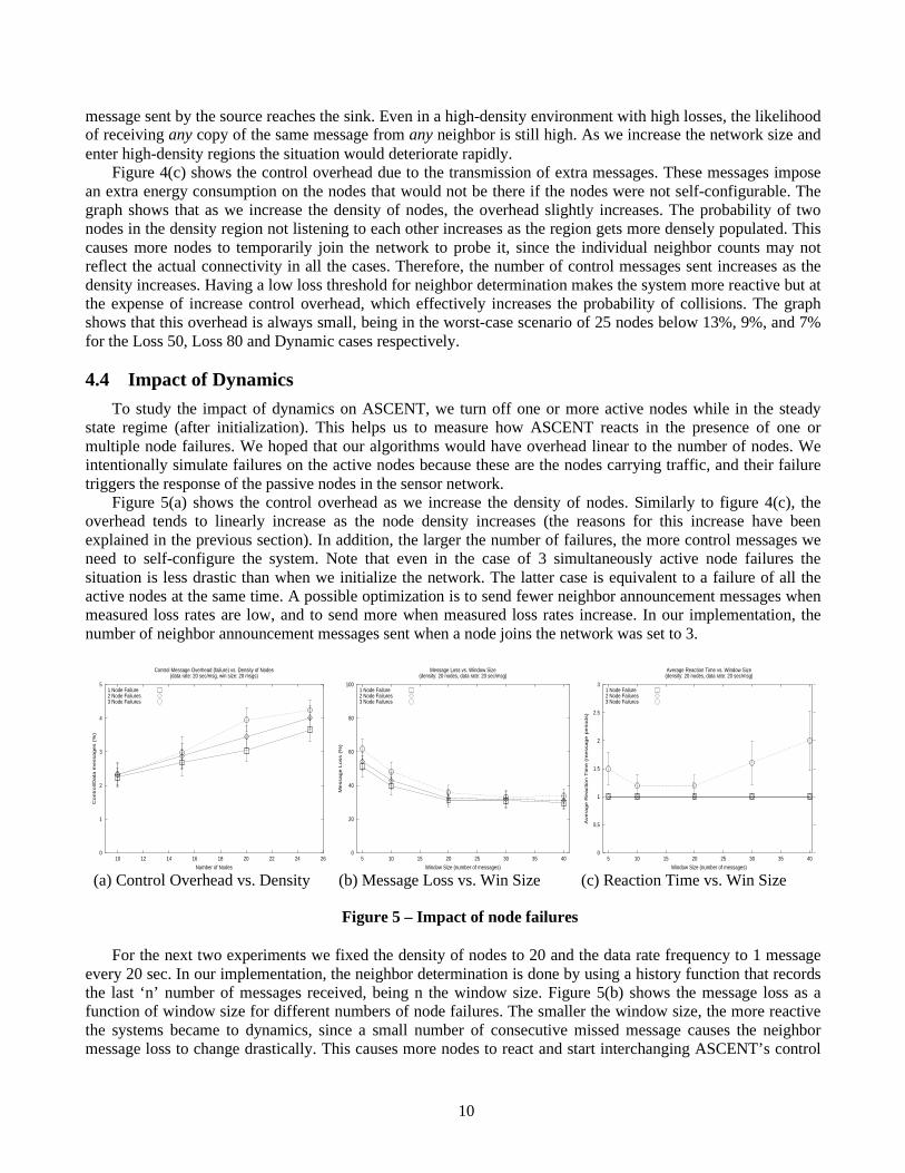
Figure 5(a) shows the control overhead as we increase the density of nodes. Similarly to figure 4(c), the overhead tends to linearly increase as the node density increases (the reasons for this increase have been explained in the previous section). In addition, the larger the number of failures, the more control messages we need to self-configure the system. Note that even in the case of 3 simultaneously active node failures the situation is less drastic than when we initialize the network. The latter case is equivalent to a failure of all the active nodes at the same time. A possible optimization is to send fewer neighbor announcement messages when measured loss rates are low, and to send more when measured loss rates increase. In our implementation, the number of neighbor announcement messages sent when a node joins the network was set to 3.

0

1

2

3

4

5

10 12 14 16 18 20 22 24 26

Contr

ol/D

ata

messages (

%)

Number of Nodes

Control Message Overhead (failure) vs. Density of Nodes(data rate: 20 sec/msg, win size: 20 msgs)

1 Node Failure2 Node Failures3 Node Failures

0

20

40

60

80

100

5 10 15 20 25 30 35 40

Message L

oss (

%)

Window Size (number of messages)

Message Loss vs. Window Size(density: 20 nodes, data rate: 20 sec/msg)


0

0.5

1

1.5

2

2.5

3

5 10 15 20 25 30 35 40

Avera

ge R

eaction T

ime (

message p

eriods)

Window Size (number of messages)

Average Reaction Time vs. Window Size(density: 20 nodes, data rate: 20 sec/msg)


(a) Control Overhead vs. Density (b) Message Loss vs. Win Size (c) Reaction Time vs. Win Size

Figure 5 – Impact of node failures

For the next two experiments we fixed the density of nodes to 20 and the data rate frequency to 1 message every 20 sec. In our implementation, the neighbor determination is done by using a history function that records the last ‘n’ number of messages received, being n the window size. Figure 5(b) shows the message loss as a function of window size for different numbers of node failures. The smaller the window size, the more reactive the systems became to dynamics, since a small number of consecutive missed message causes the neighbor message loss to change drastically. This causes more nodes to react and start interchanging ASCENT’s control

11

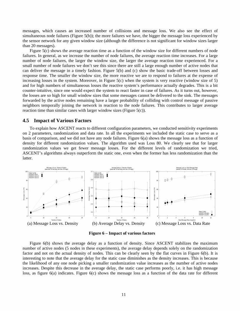
messages, which causes an increased number of collisions and message loss. We also see the effect of simultaneous node failures (Figure 5(b)); the more failures we have, the bigger the message loss experienced by the sensor network for any given window size (although the difference is not significant for window sizes larger than 20 messages).

Figure 5(c) shows the average reaction time as a function of the window size for different numbers of node failures. In general, as we increase the number of node failures, the average reaction time increases. For a large number of node failures, the larger the window size, the larger the average reaction time experienced. For a small number of node failures we don’t see this since there are still a large enough number of active nodes that can deliver the message in a timely fashion. Figure 5(b) and (c) show the basic trade-off between losses and response time. The smaller the window size, the more reactive we are to respond to failures at the expense of increasing losses in the system. Moreover, in Figure 5(c) when the system is very reactive (window size of 5) and for high numbers of simultaneous losses the reactive system’s performance actually degrades. This is a bit counter-intuitive, since one would expect the system to react faster in case of failures. As it turns out, however, the losses are so high for small window sizes that some messages cannot be delivered to the sink. The messages forwarded by the active nodes remaining have a larger probability of colliding with control message of passive neighbors temporally joining the network in reaction to the node failures. This contributes to larger average reaction time than similar cases with larger window sizes (Figure 5(c)).

4.5 Impact of Various Factors

To explain how ASCENT reacts to different configuration parameters, we conducted sensitivity experiments on 2 parameters, randomization and data rate. In all the experiments we included the static case to serve as a basis of comparison, and we did not have any node failures. Figure 6(a) shows the message loss as a function of density for different randomization values. The algorithm used was Loss 80. We clearly see that for larger randomization values we get fewer message losses. For the different levels of randomization we tried, ASCENT’s algorithms always outperform the static one, even when the former has less randomization than the latter.

0

20

40

60

80

100

5 10 15 20 25

Message L

oss (

%)

Number of Nodes

Message Loss vs. Density of Nodes(data rate: 20 sec/msg, win size: 20 msgs)

Static ConfigASCENT rand 5ASCENT rand 10ASCENT rand 15

0.2

0.3

0.4

0.5

0.6

0.7

5 10 15 20 25

Avera

ge D

ela

y (

sec)

Number of Nodes

Average Delay vs. Density of Nodes(data rate: 20 sec/msg, win size: 20 msgs)

Static ConfigASCENT rand 5ASCENT rand 10ASCENT rand 15

0

20

40

60

80

100

0 2 4 6 8 10 12

Message L

oss (

%)

Data Message Rate (msg/min)

Message Loss vs. Data Message Rate(density: 20 nodes, win size: 20 msgs)

Static ConfigASCENT DynamicASCENT Loss 80

(a) Message Loss vs. Density (b) Average Delay vs. Density (c) Message Loss vs. Data Rate

Figure 6 – Impact of various factors

Figure 6(b) shows the average delay as a function of density. Since ASCENT stabilizes the maximum number of active nodes (5 nodes in these experiments), the average delay depends solely on the randomization factor and not on the actual density of nodes. This can be clearly seen by the flat curves in Figure 6(b). It is interesting to note that the average delay for the static case diminishes as the density increases. This is because the likelihood of any one node picking a smaller randomization value increases as the number of active nodes increases. Despite this decrease in the average delay, the static case performs poorly, i.e. it has high message loss, as figure 6(a) indicates. Figure 6(c) shows the message loss as a function of the data rate for different

12

versions of ASCENT and static cases. For all the cases we see that as we increase the data rate, the message loss increases accordingly.

5 Related Work Our work has been informed and influenced by a variety of other research efforts. K. Sohrabi and G. Pottie [26] have made significant progress in self-configuration and synchronization in

sensor networks at the single cluster level with a TDMA scheme. This work shares with us similar design principles, although it’s more focused on low-level synchronization necessary for network self-assembly, while we concentrate on efficient multi-hop topology formation.

J. L. Gao’s thesis [11] presented an adaptive local network formation/routing algorithm that facilitates cooperative signal processing. An election algorithm is used to select a central node among a small group of nodes that cooperate in information processing. While these algorithms were designed to operate for a relatively short time span in a reduced area near the target event, our objective is stable, long range topology formation that covers the entire sensor network.

The adaptive techniques we use were studied extensively to make the MAC layer self-configuring and adaptive more than 20 years ago during the refinement of contention protocols. More recently SRM [9] and RTCP [25] borrowed these techniques to adaptively adjust parameters such as session message frequency and randomization intervals. In this work we use those techniques to adapt the topology of a multi-hop wireless network.

Mobile ad-hoc networks [14, 17, 19] and Diffusion [12] adaptively configure the routing or data dissemination paths, but they do not adapt the basic topology. Qun Li and Daniela Rus [15] presented a scheme where mobile nodes modify their trajectory to transmit messages in the context of disconnected ad-hoc networks. This work shares with us the notion of adaptation of the basic topology for efficient delivery of messages, but it does so sending location updates between neighbors and using active messages to incrementally propagate them toward the destination. Our work uses measurements of neighbor density and message loss to exploit the redundancy of highly dense areas in the system in an energy efficient way. This work may complement ours in case of mobile nodes deployment and in the presence of network partitions. Ramanathan et. al. [23] proposed some distributed heuristics to adaptively adjust node transmit powers in response to topological changes caused by mobile nodes. This work assumes that a routing protocol is running at all times and provides basic neighbor information that is used to dynamically adjust transmit power. In our case, ASCENT decides which nodes should run the routing algorithm, and it makes this determination based on message loss in addition to density. Similarly, Ya Xu et. al. [27] also modify the topology in response to local measurements of density. Nevertheless, it uses geographic information, and it is not based strictly on measurements of message loss.

Self-configuration based on local measured parameters takes some inspiration from biological systems, in particular the models of ant colony behavior [4]. Bulusu et. al. [3], have proposed different algorithms for incremental beacon placement in sensor networks. This work share with us the same design principles, such us the use of localized algorithms, and adaptation based on locally measured parameters. While their work is oriented to solve the localization problem, ours is more oriented to energy efficient communication coverage.

Several centralized approaches have been developed to find optimal solutions for the localization, communication coverage, and other similar problems. Doherty et. al. [5] presented a method for estimating unknown node positions based exclusively on connectivity-induced constraints. These techniques could be adapted to find an optimal solution to the communication coverage problem based on location estimates. A novel theorem in combinatorial geometry that leads to a family of approximation algorithms for the geometric disk-covering problem has been proposed in [10]. It derives a centralized solution to find the minimum number of disk to cover certain points in the network. These points could be the nodes that experience high message loss, and the placement of the disks could represent the location of the nodes to be activated. This work provides very useful bounds to what is achievable but is not intended for application to energy-constrained contexts where the cost of extracting the information about node state to a central site is prohibitive. Moreover, the radio

13

propagation characteristics may not be always best represented as disks of a certain radius. The work is being extended to distributed forms and may complement our work at a future date.

6 Conclusions and Future Work In this paper, we described the design, implementation, and experimental evaluation of ASCENT, an

adaptive self-configuration topology mechanism for distributed wireless sensor networks. There are many lessons we can draw from our preliminary experimentation. First, ASCENT has the potential for significant reduction of message loss and increase in energy efficiency. Even without optimizing parameter selection ASCENT outperforms the static scheme. Second, ASCENT mechanisms were responsive and stable under systematically varied conditions.

In the near future, we will perform experiments with larger numbers of nodes to further explore the scalability of our algorithms. We will also explore the use of wider area links to detect network partitions. In the longer term, we will explore more generally the limitations of localized algorithms and their relation to global information in the context of self-configurable sensor networks. We will also expand this work to address other modalities beyond communication coverage, such us, actuation or sensing.

This work is an initial foray into the design of self-configuring mechanisms for wireless sensor networks. Our distributed sensing network experiments represent a non-trivial exploration of the problem space. Such techniques will find increasing importance as the community seeks ways to exploit the redundancy offered by cheap, widely available microsensors, as a way of addressing new dimensions of network performance such as network-lifetime.

References [1] B. Badrinath, M. Srivastava, K.Mills, J.Scholtz, and K.Sollins, Eds. Special Issue on Smart Spaces and Environments. IEEE Personal

Communications, Oct. 2000. [2] J. Broch, D. Maltz, D. Johnson, Y.-C. Hu, and J. Jetcheva. A Performance Comparison of Multi-Hop Wireless Ad-Hic Network Routing Protocols.

In Proceedings of the Fourth Annual ACM/IEEE International Conference on Mobile computing and Networking (Mobicom’98), Dallas, TX, 1998. [3] N. Bulusu, J. Heidemann and D. Estrin. AdaptiveBeaconPlacement. In Proceedings of the Twenty First International Conference on Distributed

Computing Systems (ICDCS-21), Phoenix, Arizona, USA. April 16-19 2001. To Appear. [4] G. Di Caro and M. Dorigo. AntNet: A Mobile Agents Approach to Adaptive Routing. Technical Report 97-12, IRIDIA, Universite’ Libre de

Bruxelles, 1997. [5] L. Doherty, K. S. J. Pister, L. El Ghaoui. Convex Position Estimation in Wireless Sensor Networks. In Proceedings IEEE Infocom 2001, Anchorage

AK, April 2001. [6] J. Elson and D. Estrin. Random, Ephemeral Transaction Identifiers in Dynamic Sensor Networks. In Proceedings of the Twenty First International

Conference on Distributed Computing Systems (ICDCS-21), Phoenix, Arizona, April 2001. To appear. [7] D. Estrin, R. Govindan, and J. Heidemann, Eds. Special Issue on Embedding the Internet. Communications of the ACM, vol. 43, no. 5, May 2000. [8] D. Estrin, R. Govindan, J. Heidemann, and S. Kumar. Next century challenges: Scalable Coordination in Sensor Networks. In Proceedings of the

Fifth Annual International Conference on Mobile Computing and Networks (MobiCOM ’99), August, 1999, Seattle, Washington [9] S. Floyd, V. Jacobson, C-G. Liu, S. McCanne, and L. Zhang. A Reliable Multicast Framework for Lightweight Sessions and Application Level

Framing. IEEE/ACM Transactions on Networking, November 1997. [10] M. Franceschetti, M. Cook, and J. Bruck. A Geometric Theorem for Approximate Disk Covering Algorithms. Technical Report ETR035, Caltech

University, January 2001. [11] J. Gao. Energy Efficient Routing for Wireless Sensor Networks. PhD thesis in Electrical Engineering. University of California Los Angeles (UCLA).

August 2000. [12] C. Intanagonwiwat, R. Govindan, and D. Estrin. Directed Diffusion: A Scalable and Robust Communication Paradigm for Sensor Networks. In

Proceedings of the Sixth Annual International Conference on Mobile Computing and Networking (MobiCOM 2000), Boston, Massachusetts, August 2000

[13] V. Jacobson. Congestion Avoidance and Control. Proceedings of SIGCOMM ’88, pages 314-329. Palo Alto, CA, August 1988. [14] D. Johnson and D. Maltz. Dynamic Source Routing in Ad-hoc Wireless Networks. In T. Imielinski and H Korth, editors, Mobile Computing, pages

153-181. Kluwer Academic Publishers, 1996. [15] Q. Li and D. Rus. Sending Messages to Mobile Users in Disconnected Ad-hoc Wireless Networks. In Proceedings of the Sixth Annual International

Conference on Mobile Computing and Networking (MobiCOM 2000), pages 44-55, Boston, August 2000. [16] R. Metcalfe and D. Boggs. Ethernet: Distributed Packet Switching for Local Computer Networks. Communications of the ACM, 19 (5): 395-404,

July 1976. [17] V. Park and M. Corson. A Highly Adaptive Distributed Routing Algorithm for Mobile Wireless Networks. In Proceedings of INFOCOM 97, pages

1405-1414, April 1997 [18] PC-104 Consortium, http://www.pc104.org [19] C. Perkins and E. Royer. Ad hoc On-Demand Distance Vector Routing. Proceedings of the 2nd IEEE Workshop on Mobile Computing Systems and

Applications, New Orleans, LA, February 1999, pp. 90-100. [20] G. Pottie and W. Kaiser. Wireless Integrated Network Sensors. Communications of the ACM, 43 (5): 51-58, May 2000. [21] Radio Packet Controller, http://www.radiometrix.com

14

[22] RPC Linux driver, http://www.circlemud.org/~jelson/software/radiometrix [23] S. Ramanathan and R. Rosales-Hain. Topology Control of Multihop Radio Networks using Transmit Power Adjustment. In Proceedings of IEEE

Infocom 2000, Tel Aviv, Mar 2000. [24] Sensors: The Journal of Applied Sensing Technology. [25] H. Schulzrinne, S. Casner, R. Frederick, and V. Jacobson. RFC 1889 RTP: A Transport Protocol for Real-Time Applications. Standards Track.

January 1996. [26] K. Sohrabi and G. Pottie. Performance of a Novel Self-Organization Protocol for Wireless Ad-Hoc Sensor Networks. In Proceedings of IEEE VTC,

Amsterdam, Netherlands, September 1999. [27] Y. Xu, J. Heidemann, and D. Estrin. Adaptive Energy-Conserving Routing for Multihop Ad Hoc Networks. Research Report 527, USC/Information

Sciences Institute, October 2000.

ascent: adaptive self-configuring sensor … ascent: adaptive self-configuring sensor networks...

Documents