assessment of greenhouse gas emissions in the production ... · 33 assessment of greenhouse gas...
TRANSCRIPT

33
Assessment of greenhouse gasemissions in the production
and use of fuel ethanol in Brazil
Government of the State of São Paulo
Geraldo Alckmin – Governor
Secretariat of the Environment
José Goldemberg – Secretary
Isaias de Carvalho Macedo – Núcleo Interdisciplinar de PlanejamentoEnergético da Universidade Estadual de Campinas – NIPE/UNICAMP
Manoel Regis Lima Verde Leal – Centro de TecnologiaCopersucar (CTC/Copersucar), Piracicaba
João Eduardo Azevedo Ramos da Silva – Centro de TecnologiaCopersucar (CTC/Copersucar), Piracicaba
March 2004
5
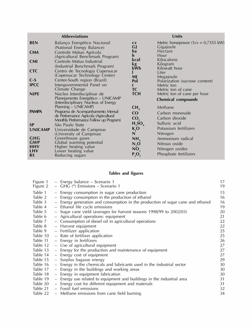
cv Metric horsepower (1cv = 0,7355 kW)GJ Gigajouleha Hectareh Hourkcal Kilocaloriekg KilogramkWh Kilowatt hourl LiterMJ MegajoulePol Polarization (sucrose content)t Metric tonTC Metric ton of caneTCH Metric ton of cane per hour
Chemical compounds
CH4 MethaneCO Carbon monoxideCO2 Carbon dioxideH2SO4 Sulfuric acidK2O Potassium fertilizersN NitrogenNH4 Ammonium radicalN2O Nitrous oxideNOx Nitrogen oxidesP2O5 Phosphate fertilizers
BEN Balanço Energético Nacional(National Energy Balance)
CMA Controle Mútuo Agrícola(Agricultural Benchmark Program)
CMI Controle Mútuo Industrial(Industrial Benchmark Program)
CTC Centro de Tecnologia Copersucar(Copersucar Technology Center)
C-S Center-South region (Brazil)IPCC Intergovernmental Panel on
Climate ChangeNIPE Núcleo Interdisciplinar de
Planejamento Energético – UNICAMP(Interdisciplinary Nucleus of EnergyPlanning – UNICAMP)
PAMPA Programa de Acompanhamento Mensalde Performance Agrícola (AgriculturalMonthly Performance Follow up Program)
SP São Paulo StateUNICAMP Universidade de Campinas
(University of Campinas)GHG Greenhouse gasesGWP Global warming potentialHHV Higher heating valueLHV Lower heating valueRS Reducing sugars
Tables and figures
Figure 1 – Energy balance – Scenario 1 17Figure 2 – GHG (*) Emissions – Scenario 1 19
Table 1 – Energy consumption in sugar cane production 15Table 2 – Energy consumption in the production of ethanol 16Table 3 – Energy generation and consumption in the production of sugar cane and ethanol 16Table 4 – Ethanol life cycle emissions 19Table 5 – Sugar cane yield (averages for harvest seasons 1998/99 to 2002/03) 20Table 6 – Agricultural operations: equipment 21Table 7 – Consumption of diesel oil in agricultural operations 22Table 8 – Harvest equipment 22Table 9 – Fertilizer application 25Table 10 – Rate of fertilizer application 25Table 11 – Energy in fertilizers 26Table 12 – Use of agricultural equipment 27Table 13 – Energy for the production and maintenance of equipment 27Table 14 – Energy cost of equipment 27Table 15 – Surplus bagasse energy 29Table 16 – Energy in the chemicals and lubricants used in the industrial sector 30Table 17 – Energy in the buildings and working areas 30Table 18 – Energy in equipment fabrication 30Table 19 – Energy use related to equipment and buildings in the industrial area 31Table 20 – Energy cost for different equipment and materials 31Table 21 – Fossil fuel emissions 32Table 22 – Methane emissions from cane field burning 34
Abbreviations Units

7
Contents
Preface 9
Executive summary 10
Introduction 11
Objective 11
Methodology 11
Database 12
Systems and emission flows definition 13
Emissions
Use of fossil fuel in sugar cane production 15
Use of fossil fuel in the industrial production of ethanol 15
GHG emissions due to the use of fossil fuels 17
Other GHG emissions in the production and use of ethanol 17
Avoided emissions 18
Balance of emissions and conclusion 18
Annexes
Annex 1: Sugar cane production 20
Annex 2: Use of energy in the industrial processing of cane to ethanol 28
Annex 3: Notes and supplementary data 32
References 37

9
Preface
O ne of the main tasks of the Secretariat of the Environment of the State of São Paulo is the improvement of air quality in the State’s urban areas. The addition to gasoline of 20-25% of ethanol is an
important contribution to this end.
The substitution of gasoline by alcohol has another importantconsequence: the reduction of greenhouse gas emission (principally CO2)provided that in the production of the ethanol, the fossil fuel contribution isminimized. This contribution stems from the energy needed to producethe raw materials used in farming and in the industrial process (fertilizers,lime, sulfuric acid, lubricants etc.) as well as electricity and fuels acquiredby the producer (direct energy consumptions).
To consider ethanol as a renewable (or an “almost renewable”)fuel, it is essential that the production fossil fuels’ contribution is small, justas with the emission of greenhouse gases not directly associated with theuse of fossil fuels in the entire cycle of production and usage.
Along the years evaluations of this contribution have been madeby various groups of specialists, with highly encouraging results.
With the increase in the numbers of ethanol production units andwith the advances of technology, the Secretariat of the Environment felt itto be necessary to seek from University of Campinas (UNICAMP) anupdating of these evaluations. This update was carried out with dataobtained also from the Copersucar Technology Center (CTC/Copersucar).This report is the result of this work.
Prof. José Goldemberg
Secretary of the Environment
1010
S
10
Executive summary
ugar cane energy products, ethanol andbagasse, have made a significant contributionto the reduction of greenhouse gas (GHG)emissions in Brazil, substituting fossil fuels,gasoline and fuel oil, respectively.
However, fossil fuels are used in theoperations of planting, harvesting, transportationand processing of the sugar cane, resulting inGHG emissions. Energy and GHG balancesare required to evaluate the net effects duringthe complete well-to-wheel cycle of ethanol,i.e. ethanol production from sugar cane and itsuse as fuel in the transport sector. To facilitatethe comparison with other studies, the GHGdata are presented as CO2 equivalentemissions (CO2eq.).
In the energy balance three levels ofenergy flows are considered, making it easierto compare with other energy balances.Level 1 – Only the direct consumption ofexternal fuels and electricity (direct energyinputs) is considered.Level 2 – This is the additional energyrequired for the production of chemicals andmaterials used in the agricultural andindustrial processes (fertilizers, lime, seeds,herbicides, sulfuric acid, lubricants, etc.).Level 3 – This is the additional energynecessary for the manufacture, constructionand maintenance of equipment and buildings.
Due to the diversity of the databasefor the technical parameters related to thesugar cane and ethanol production in Brazil,a limited but reliable database was preparedusing the information available at Copersucar.This database has the advantage of traceabilityand consistent references.
Two cases have been considered in theevaluation of energy flows: Scenario 1 based on theaverage values of energy and material consumptionand Scenario 2 based on the best values beingpracticed in the sugar cane sector (minimumconsumption with the use of the best technology inuse in the sector). In both Scenarios the balance isreferred to one metric ton of cane (TC).
Under these conditions, the results obtainedfor energy consumption were: 48,208 kcal/TC and45,861 kcal/TC in the agricultural sector forScenarios 1 and 2, respectively, and 11,800 kcal/TC and 9,510 kcal/TC in the industrial sector forScenarios 1 and 2, respectively. The total energyconsumptions for Scenario 1, 60,008 kcal/TC, andScenario 2, 55,371 kcal/TC, compare very favorablywith the total energy production (ethanol and surplusbagasse) of 499,400 kcal/TC and 565,700 kcal/TC,for Scenarios 1 and 2, respectively. The ratios ofoutput energy (renewable) to input energy (fossil)are 8.3 and 10.2, for Scenarios 1 and 2, respectively.
In the GHG balance the emissions havebeen divided into two groups: emissions derivedfrom the use of non renewable energy (diesel andfuel oil) and emissions from other sources (cane trashburning, fertilizer decomposition).
For the first group the calculated values were19.2 kg CO2eq./TC and 17.7 kg CO2eq./TC forScenarios 1 and 2, respectively, while the valuesdetermined for the second group were 12.2 kgCO2eq./TC for both Scenarios.
The emissions avoided due to the substitutionof ethanol for gasoline and surplus bagasse for fueloil, deducting the above values, gives a net resultof 2.6 and 2.7 t CO2eq./m3 anhydrous ethanol and1.7 and 1.9 t CO2eq./m3 of hydrous ethanol, forScenarios 1 and 2, respectively.

11
T
Introduction
he Brazilian sugar cane agribusiness is aneconomic activity responsible for 2.2% ofGDP, generating an income of over US$ 8billion and creating approximately onemillion direct jobs: more than 400,000 in theState of São Paulo alone – the country’slargest producer State – as well as fosteringthe economic development of a largenumber of municipalities and contributing tothe employment of a large number ofworkers in the rural areas.
The activity has a positive envi-ronmental differential that is the efficientproduction of fuel grade ethanol from sugarcane. The extensive use of fuel ethanol inBrazil, whether as a 25% blend with gasoline(gasohol), or used as a neat fuel in vehiclesequipped with dedicated alcohol engines orused in the newly produced flex fuelvehicles, which can operate on neatethanol, gasohol or any intermediate blend,places Brazil as a leader in carbon emissionreduction and Greenhouse Effect mitigation.
The production of ethanol in the 2003/2004 crop season will reach the significantvolume of 14.4 billion liters and the Center-South region, which includes São Paulo State,will respond for 89.6% of the total.
In addition to the production ofethanol, the industrial processing of sugarcane generates bagasse, another valuableproduct. This residue also adds to theindustry’s positive environmental differentialbecause it has been widely used to replacefossil fuels in the production of industrial heatand electricity in the sugar mills anddistilleries thereby boosting the abatementpotential of greenhouse gases emission.
The present work is a contribution toa better understanding of the renewableenergy value and energy efficiency of thisimportant industrial sector.
Objective
This work presents the life cycleanalysis of the GHG emissions in theproduction and use of ethanol, under thetypical conditions found in Brazilian sugar
and ethanol mills. It also presents the emissionsderived from fossil fuel consumption and those notrelated to the use of energy.
Data collected in 2002 have been used forthe latest update of the analysis of energy consumptionin the sugar cane ethanol production at Copersucarmills undertaken in 19851, then updated in 19982.
The observations made in the first report,especially those concerning the correct definitionof the boundaries of the process analysed, remainvalid. Some of the parameters defined at that timehave been maintained in this report, due to thedifficulties found in their updating. However this factcan be considered of little importance since it wouldhave only a very small impact on the energyconsumption figures.
The evaluation of the GHG emissions in theproduction and use of ethanol is also an update anda revision of previous work performed at theCopersucar Technology Center (CTC), whose studieswere published in 19923 and revised in 1998, with1996 data4.
Methodology
The energy flows have been considered intwo situations: one (Scenario 1), based on the averagevalues of energy and chemicals’ utilizations, and theother (Scenario 2), based on the best existing values(minimum consumption values resulting from theapplication of the best technology in use by thesector). The use of these scenarios allows not onlythe characterization of the present situation (Scenario1) but also the estimation of a situation that maybecome reality in the medium term (Scenario 2) bythe widespread use of good practices already beingused in some mills. Technologies that are alreadydeveloped, or in the process of being developed, butare not used in a significant degree today, have notbeen considered in this work.
Technologies in the process of gradualintroduction, that may have significant impact onthe GHG emissions, have been considered at thepresent degree of utilization. This is the case ofmechanically harvested unburned cane, withouttrash recovery for power generation.
The energy flows have been consideredin three levels, to facilitate the comparison withother studies:

12
Level 1 – Only the direct consumptions of external fuelsand electricity (direct energy inputs) are considered.Level 2 – The energy required for the production ofchemicals and materials used in the agricultural andindustrial processes (fertilizers, lime, seeds,herbicides, sulfuric acid, lubricants etc.) is added.Level 3 – The energy necessary for the fabrication,construction and maintenance of equipment andbuildings is added.
The parameter values recommended by theIntergovernmental Panel on Climate Change (IPCC)7
have been used in the GHG emission calculationswhenever available.
Database
A complete countrywide database for thesugar cane sector has not yet been fully established,thus the use of a database covering part of the sectorbut based on reliable and traceable information hasbeen preferred. It is important to point out that thisdatabase is representative of the agricultural andindustrial practices, especially of the Center-Southregion, accounting for approximately 85% of thesugar cane production in Brazil.
Under these considerations the followingdocuments have been selected as references for theenergy balance of ethanol production in Brazil.
– Copersucar: Agricultural Benchmark Program (26to 31 mills in the State of São Paulo) – These reportspresent dozens of performance parameters in theagricultural sector of a group of Copersucarassociated mills. They have been prepared for manyyears, bring monthly and annual averages, and havebeen fully discussed among the participating mills.– Copersucar: Industrial Benchmark Program (17 to22 mills in the State of São Paulo) – These reportspresent the industrial sector performance parameters(efficiencies, consumption of chemicals etc.) of aselected part of Copersucar member mills. They havebeen also extensively discussed among the participants,and show the monthly and annual averages.– Copersucar: Agricultural Monthly PerformanceFollow up Program (98 mills in the Center-Southregion) – These reports present the agriculturalsector parameters for a larger number ofparticipating mills in the Center-South region.However the traceability of the information andthe uniformity of procedures have not the samelevel of accuracy as in the cases of the twoprevious sets of documents.
In the cases where weather conditions canhave significant impacts on the results (such as thecase of sugar cane productivity) the averages forfive seasons in sequence (1998/99 to 2002/2003seasons) have been used. In other cases, the 2001/2002 harvesting season has been used as referencefor both agricultural and industrial performance data.

13
T
Systems and emissionflows definition
o evaluate the GHG emission mitigation in thelife cycle of ethanol produced from sugar cane,the concept of “autonomous distillery” hasbeen adopted, meaning that the mill willprocess the sugar cane to produce ethanolonly. In this way the effects of sugar productioncan be ignored.
The mitigation corresponds to thereduction of GHG emissions obtained by theproduction and use of ethanol (substituting forgasoline as a fuel). It is, therefore, thedifference between the emissions in asituation where no ethanol is produced norused and a situation with the actual emissionswith ethanol: both of which situations reflectBrazilian conditions.
For the life cycle analysis thecontrol volume used included the caneproduction area, the distillery and the finaluse of fuel ethanol.
To facilitate the calculations theGHG emissions have been divided intofour groups.
Group 1:Carbon flows associated with the uptakeof atmospheric carbon by photosynthesisand its gradual release by oxidation.1.a Uptake of atmospheric carbon(photosynthesis);1.b Carbon release during cane field burning,before harvesting (around 80% of tops andleaves are burned with an efficiency of 90%);1.c Oxidation of unburned residues, inthe field;1.d CO2 release in the fermentation ofsucrose to ethanol;1.e CO2 release by the combustion of allbagasse, for power and heat generation, inthe boilers of the mills or in other industriesboilers (surplus bagasse);1.f CO2 release by the combustion of ethanolin automobile engines.
These emission flows can be con-sidered to be nearly neutral, for it is assumedthat all fixed carbon is released again withinthe cycle of sugar cane production and thefinal use of ethanol and bagasse. An exceptionis the uptake of part of the carbon in the soil (inpast decades the cane fields showed a positiveaverage carbon uptake because land was
generally poor in organic matter before being used togrow cane). In this study, due to the difficulties inestimating with a minimum accuracy the level ofcarbon fixed in the soil, this fraction has been ignored,which results in a conservative assumption.
Thus, the net contribution of the Group 1 carbonflows has been considered as zero which is a commonassumption for cycles of biomass production and use.
Group 3:The GHG flows not associated with the use of fossilfuels are mainly N2O and methane; considerationwas given to:3.a Release of other GHG (non CO2) in the processof cane field burning;3.b Release of N2O from the soil, due to fertilizerdecomposition;3.c Release of other GHG (non CO2) in the combus-tion of bagasse in steam boilers;3.d Release of other GHG (non CO2) in the combus-tion of ethanol in engines.
These are negative flows since they contributeto emission increase.
These flows are also negative, that is, theycontribute to the increase of GHG emissions.
Group 2:Carbon flows associated with the use of fossil fuelsin the production of all chemicals and inputs usedin the agricultural and industrial sectors for theproduction of sugar cane and ethanol, as well as inthe manufacture of equipment, construction ofbuildings and their maintenance:2.a CO2 release due to the use of fossil fuels in thecane fields: tillage, irrigation, harvesting, transpor-tation etc.;2.b CO2 release due to the use of fossil fuels in theproduction of agricultural inputs (seeds, herbicides,pesticides, fertilizers, lime etc.);2.c CO2 release due to the use of fossil fuels in theproduction of agricultural equipment, spare partsand their maintenance;2.d CO2 release due to the use of fossil fuel forindustrial inputs (lime, sulfuric acid, biocides, lu-bricants etc.);2.e CO2 release due to the use of fossil fuels in themanufacture of equipment, construction of buil-dings, and their maintenance in the industrial area.

14
Group 4:This group includes what can be called “virtual”flows of GHG emissions; they would take place if,in the absence of ethanol, the fuel demand wasmet by gasoline and if in the absence of surplusbagasse, fuel oil was used.These emissions can be characterized as:4.a GHG avoided emission by substituting ethanolfor gasoline;4.b GHG avoided emission by substituting bagassefor fuel oil in other industrial sectors.
In the analysis that follows, the flows of Groups2 to 4 will be evaluated; the flows of Group 1 will notbe calculated since the net balance is zero. To facilitatethe understanding of some simplifying assumptions, it isimportant to bear in mind that the emissions of Groups2 and 3 are nearly ten times smaller than those of Group4. This is normally true for fossil fuels or biomass systemswhere the energy embodied in equipment and buildingsis small when the whole useful life is considered. Thesame applies to the energy inputs for the manufactureof chemicals and other materials used in the productionprocess. There are some exceptions such as the caseof ethanol from corn in the USA.
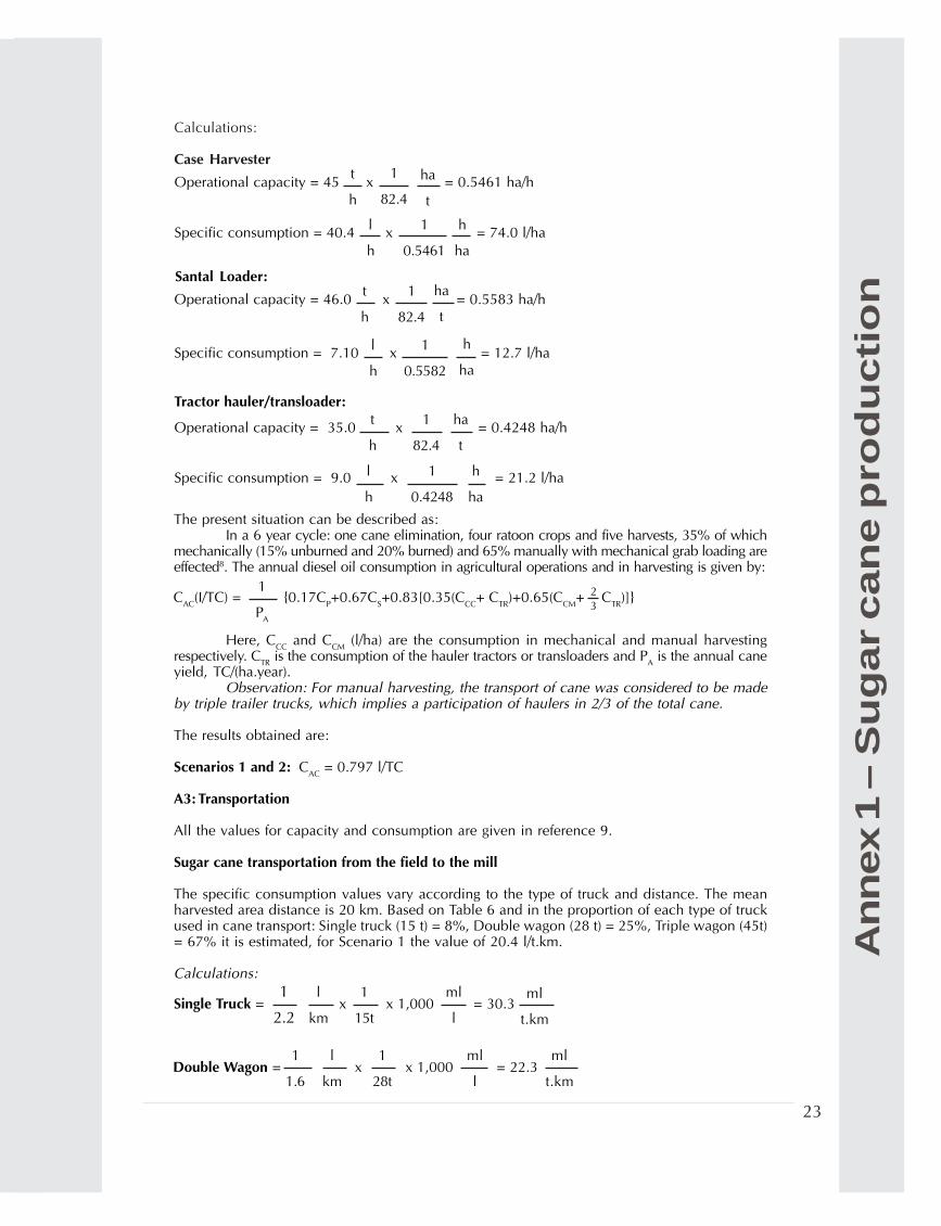
15
T
Level Energy consumptionScenario 1 Scenario 2 (kcal/TC) (kcal/TC)
FuelAgricultural operations/harvesting (A2)Transportation (A3)Level total
Fertilizers (A4)Lime (A5)HerbicidePesticidesSeeds (A6)Level total
Equipment (A7)Level total
Total
Table 1 – Energy consumption in sugar cane production
1
2
3
9,0978,720
17,817
15,1521,7062,690
1901,336
21,074
6,9706,970
45,861
9,09710,26119,358
15,8901,7062,690
1901,404
21,880
6,9706,970
48,208
Emissions
he detailed analysis is presented in Annex1. The three energy levels considered insugar cane production are:Level 1 – Diesel oil used in agriculturaloperations and sugar cane transportation.Level 2 – Other inputs: fertilizers, lime,herbicides, pesticides, seeds.Level 3 – Energy for production andmaintenance of equipment and labor.
In Level 1, the energy consumptionassociated to fuel (diesel) can be calculatedusing the energy value of diesel (lower heatingvalue, LHV = 9,235 kcal/l plus 2,179 kcal/l forproduction, transportation and processing) of11,414 kcal/l. It should be pointed out that if theobjective of the analysis was just to verify thefraction of self consumption of the same type ofenergy in the ethanol production, without regardto the life cycle, the diesel use should beconsidered as its LHV value. For fuel oil theenergy values are equivalent to diesel5. Someadditional comments on these values can befound in Annex 3, Note 1.
The summary of the results ispresented in Table 1. In this summary, nodistinction is made between the differentforms of energy (usually electric energyis considered at its thermodynamic value,that is, the thermal energy used in its
Use of fossil fuel insugar cane production
generation) but a complete discussion is presentedin Annex 3, Note 2.
Use of fossil fuel in the industrialproduction of ethanol
The detailed analysis is shown in Annex 2.In the industrial processing of sugar cane to
produce ethanol there are three items that shouldbe considered in the final energy balance:Level 1 – Purchased electric energy, if any.Level 2 – Energy required for the production of inputsto the industrial process (chemicals, lubricants).Level 3 – Energy for the manufacture of equipment,construction of buildings and their maintenance.Table 2 summarizes the results for the three levelsand two Scenarios without distinction between theforms of energy (see Annex 3, Note 2).
It can be seen from the energy balance (Annex2) that there is a surplus of energy being produced, inthe form of surplus bagasse that will be considered inthe overall analysis, amounting to 40,300 kcal/TC(Scenario 1) or 75,600 kcal/TC (Scenario 2).A comparison between the energy produced in theprocess in the form of ethanol and surplus bagasseand the fossil energy consumed is shown in Table3. It can be seen that the output energy to input

16
Table 3 – Energy generation and consumption in the production of sugar cane and ethanol
Activity Energy consumption
Scenario 1 Scenario 2(kcal/TC) (kcal/TC)
Sugar cane production (total)
Agricultural operations
Transportation
Fertilizers
Lime, herbicides, pesticides etc.
Seeds
Equipment
Ethanol production (total)
Electricity
Chemicals, lubricants
Buildings
Equipment
External energy flows Input Output Input Output
Agriculture 48,208 - 45,861 -
Factory 11,800 - 9,510 -
Ethanol produced - 459,100 - 490,100
Surplus bagasse - 40,300 - 75,600
Total 60,008 499,400 55,371 565,700
Output/input 8.3 10.2
48,208 45,861
9,097 9,097
10,261 8,720
15,890 15,152
4,586 4,586
1,404 1,336
6,970 6,970
11,800 9,510
0 0
1,520 1,520
2,860 2,220
7,420 5,770
energy ratio is 8 to 10, considerably larger than in thecase of ethanol from corn in the USA. The energy flows
in and out of the control volume of the agricultural andindustrial sectors are shown in Figure 1, for Scenario 1.
1
2
3
Table 2 – Energy consumption in the production of ethanol
Level Energy consumptionScenario 1 Scenario 2(kcal/TC) (kcal/TC)
Electric energy
Chemicals and lubricants (A9)
Buildings (A10)Heavy equipmentLight equipment
Total
0
1,520
2,8603,4703,950
11,800
0
1,520
2,2202,7003,070
9,510

17
Figure 1 – Energy balance – Scenario 1 (Mcal/TC)
Agricultural area(Sugar cane production)
Industrial area(Processing of ethanol)
Surplusbagasse
40.3
Ethanol459.1
1 t cane
Fertilizer 15.9Lime 1.7Herbicides 2.7Pesticides 0.2Seeds 1.4
Manufacture/maintenanceequipment 7.0
Chemicallubricants 1.5
Manufacture/maintenanceBuildings 2.9Heavy equipment 3.5Ligth equipment 4.0
Electric energy 0Thermal energy 0
Solar energy
Agricultural operations 9.1Transportation 10.3
(Renewable energy)/(Fossil lubricants) = 8.3
GHG emissions due to the use of fossil fuels
All fossil fuel use listed in Tables 1 and 2 hasbeen considered here, including direct and indirectuses. The values of indirect uses of energy for fuels,as well as the carbon emission coefficients for theircombustion, can be found in Annex 3, Note 2.
Diesel has been considered in the agricul-tural operations, cane harvesting and trans-portation and fuel oil for the production ofchemicals and the energy embodied in equipment,buildings and their maintenance. This sim-plification is acceptable considering the structureof the energy use in such applications and the smallmagnitudes involved.
Total diesel oil consumption: 19,358 kcal/TCand 17,817 kcal/TC, for Scenarios 1 and 2, respectively.
Total fuel oil consumption: 40,650 kcal/TC and370,554 kcal/TC, for Scenarios 1 and 2, respectively.
The corresponding GHG emissions, as CO2equivalent (CO2eq.), are: 19.2 and 17.7 kg CO2eq./TC, for Scenarios 1 and 2, respectively.
Other GHG emissions in the productionand use of ethanol
In this category are included the emissionsassociated with sugar cane production, cane processingfor ethanol and final use of ethanol (as fuel) that are notderived from use of fossil fuels. The most important are:– Methane and N2O emissions from the burning of sugarcane trash before harvesting;– N2O soil emissions;– Methane emissions from bagasse burning in boilers;
– Methane emissions from ethanol combustion invehicle engines, compared with those from gasolinecombustion.
Emissions from sugar cane trash burning in the field.
The calculation have been done consideringemission coefficients measured in a wind tunnelsimulating the cane field burning6 and alternativelythe average values for agricultural residuesrecommended by IPCC7 (see Annex 3, Note 4).
The IPCC values led to higher emissionsvalues and, being on the conservative side, havebeen adopted; the results for methane and N2O,shown in detail in Annex 3, Note 4, are: 9.0 kgCO2eq./TC
N2O soil emissions
Evaluations based on the use of nitrogenfertilizers (Annex 3, Note 5) considered that for theCenter-South region conditions around 28 kg N/haare used in cane planting and 87 kg N/ha for eachratoon, which gives an average value of 75 kg N/(ha.year) for the whole cane cycle. Most of thefertilizer used is of the NH4 type.
The resulting emissions are 1.76 kg N2O/(ha.year). Since N2O has a global warming potential296 larger than CO2, this results in 521 kg CO2eq./(ha.year) or 6.3 kg CO2eq./TC
Methane emissions from bagasse burning in boilers.
Significant unburned organic compoundemissions, including methane, in bagasse firedboilers take place only during operational transientsor uncontrolled disturbances in the combustion

18
process. Because of almost continuous operationduring the crop season, which is the ethanolproduction period, such transients and disturbancesare relatively small in the ethanol distilleries andsugar mills, and this substantially reduces methaneemissions. Therefore, this type of emissions will beignored in this study.
Methane emissions from automotive engines fueledwith ethanol or gasoline/ethanol blends, comparedwith those from pure gasoline engines.
It is shown in Annex 3, Note 6, that althoughit is difficult to measure differences betweenemissions from ethanol and gasoline engines (sincethere are no engines in use in Brazil that operate onethanol-free gasoline), the technological evolutionof the engines fueled with ethanol and gasoline/ethanol blends has made it possible for these enginesto meet current tight legal emission limits. It has alsobrought the methane emissions to very low levels.
These values are very small when comparedwith other items considered in this study. In Annex 3the beneficial aspects of the use of ethanol inautomobile engines are also discussed.
Avoided emissions
GHG emissions are avoided by the use ofsurplus bagasse as fuel in other industrial sectors,substituting for fuel oil, as well as by the use of ethanolas an automotive fuel, substituting for gasoline. In a nearfuture, a fraction of the bagasse produced (and the trash)could be used to generate considerable amounts ofsurplus electric energy or more ethanol, via hydrolysis,contributing even more to reducing the GHG emissions.
Surplus bagasse
An analysis of the surplus bagasse situation ispresented in Annex 3, Note 7.
On average, 280 kg of bagasse/TC areproduced with a moisture content of around 50%. Thesurplus is estimated as 8% in Scenario 1 and 15% inScenario 2; therefore, the energy corresponding tothese amounts of bagasse are 40,300 and 75,600 kcal/TC, for Scenarios 1 and 2, respectively (see Annex 2).
To estimate the avoided emissions when thisbagasse is substituting for fuel oil, operating conditionshave been established for both bagasse and fuel oilfired boilers. Under these conditions (see Annex 3,Note 7), the 8% and 15% of surplus bagassecorrespond, in terms of end energy use, to 3.2 and 6.1kg fuel oil/TC being displaced.
The total avoided emissions (includingindirect emissions) related to the fuel oil displacedare 12.5 and 23.3 kg CO2eq./TC, for Scenarios 1and 2, respectively.
Ethanol
Considering the average productivity andefficiencies of the mills and distilleries, the total emissions(direct and indirect) of the displaced gasoline (Annex 3,Note 8) and the fuel equivalence of Brazilian automobileengines, the avoided emissions due to the use of ethanolwere calculated for hydrous and anhydrous ethanol. Thedetails are presented in Annex 3, Note 8.The resulting avoided emissions are:2.82 kg CO2/l anhydrous ethanol1.97 kg CO2/l hydrous ethanolReferring to metric ton of cane, the figures are:Anhydrous ethanol: 242.5 or 259 kg CO2eq./TC, forScenarios 1 and 2, respectivelyHydrous ethanol: 169.4 or 180.8 kg CO2eq./TC, forScenarios 1 and 2, respectively.
Balance of emissions and conclusions
The results presented above are summarizedin Table 4.
The values are alternative, which means that242.5 kg CO2eq./TC is avoided if anhydrous ethanolis produced or 169.4 kg CO2eq./TC with theproduction of hydrous ethanol.
For many applications it is more convenientto have the emission data referred to as cubic metersof ethanol (net value), whether it is anhydrous orhydrous. The conversion can be done using the sugarcane productivity of the two scenarios, leading to:Anhydrous ethanol: 2.6 and 2.7 t CO2eq./m3 ethanol,for Scenarios 1 and 2 respectivelyHydrous ethanol: 1.7 and 1.9 t CO2eq./m3 ethanol,for Scenarios 1 and 2, respectively.
The values for Scenario 1 (current average),should be preferred for GHG emissions evaluationsbecause they reflect realistic conditions.
Figure 2 shows the emission flows relatedto the Agricultural Production, Industrial Processingand Ethanol Bagasse Utilization control volumes(Scenario 1).
Taking as a base case that Brazilian fuelethanol consumption is around 12 million m3 peryear, in approximately equal shares of anhydrous andhydrous ethanol, it can be estimated that the use ofethanol as a fuel in Brazil reduces the GHGemissions by 25.8 million t CO2eq./year or 7.0 milliont Carbon eq./year.

19
Figure 2 – GHG (*) Emissions – Scenario 1 (kg CO2eq./TC)
Avoided emissions: 220.5 (anhydrous ethanol) ou 147.4 (hydrous ethanol) kg CO2eq./TC
(*) Photosynthesis cycle is not included since all carbon fixed by the cane is released as CO2 (bagasse burning, burning/oxidation of trash, ethanol burning, fermentation; except for a small fraction that isfixed into the soil).
Agricultural area(Cane production)
Industrial processing(Ethanol production)
UtilizationEthanol : VehiclesSurplus bagasse : Industrial fuelSurplus
bagasse
Ethanol
1 t de cane
CH4, cane burning 6.6
N2O, from soil 6.3
N2O, cane burning 2.4
CH4, boilers (~zero)CH4 other
(~ zero with respect to gasoline)
Chemicals, etc. 7.1
Transportation andagricultural operations 6.0
Chemicals, lubricants 0.5Building, equipment 3.3
Electric and thermal energy (zero)
Surplus bagassesubstitution for fueloil: 12.5
Ethanol substitution forgasoline: 242.5(anhydrous)or 169.4 (hydrous)
Equipment 2.3
(A): Anhydrous ethanol(H): Hydrous ethanol
Table 4 – Ethanol life cycle emissions(kg CO2eq./TC)
Scenario 1 Scenario 2(average) (best values)
Type
Fossil fuels
Methane and N2O from trash burning
Soil N2O
Total emissions
Avoided emissions
Surplus bagasse use
Ethanol use
Total avoided emissions
Net avoided emissions
17.7
9.0
6.3
33.0
23.3
19.2
9.0
6.3
34.5
12.5
259.0 (A); 180.8 (H)
282.3 (A); 204.2 (H)
249.3 (A); 171.1 (H)
242.5 (A); 169.4 (H)
255.0 (A); 181.9 (H)
220.5 (A); 147.4 (H)

20
Annex 1 – Sugarcane production
20
Mechanical harvest 35%
Manual harvest 65%
Burned sugar cane harvest 80%
Unburned cane harvest 20%
Type of harvest São Paulo (%) Center-South (%)
Manual 63.8 65.2
Mechanical 36.2 34.8
Burned sugar cane 75.0 79.1
Unburned sugar cane 25.0 20.9
Table 5 – Sugar cane yield (averages for harvest seasons 1998/99 to 2002/03)
Harvest Yield (t/ha)
1st – Plant cane (18 months)
Plant cane (12 months)
2nd – (1st ratoon) 90
3rd – (2nd ratoon) 78
4th – (3rd ratoon) 71
5th – (4th ratoon) 67
Average of 5 harvests 82.4 t/ha (68.7 t/ha.year)
_} Xweighed = 106
113 (80%)
77 (20%)
Introduction
The data used in this analysis refers to the year 2002 for the Copersucar associated mills.In the present situation some of the basic parameters for harvest and sugarcane quality used were:
1. Sugar cane harvest – present situation8
Considering that approximately 85% of the Brazilian ethanol production occurs in theCenter-South, the following situation was assumed for Brazil:
For simplicity all the unburned cane harvested was considered to be mechanized harvest.It is important to mention that this simplification results in a more conservative analysis.
These data were used to determine the necessary equipment for the agricultural operations.
2. Pol and Fiber
Considering the average of five consecutive harvest seasons (1998/99 to 2002/03) thefollowing data were obtained9:
A1: Agricultural yield
The averages for various regions and sugar cane varieties (Copersucar Technology Center – CTC) are:
Average Pol % cane 14.53%
Average Fiber % cane 13.46%
Average age of plow out9:99/00 harvest season 5.13 harvests00/01 harvest season 5.18 harvests01/02 harvest season 5.33 harvests
Normally 5 harvests are carried out (average of 82.4 t/ha). The ratoons are cut after oneyear and the plant cane two years after harvesting the previous ratoon for “18 month cane”.Therefore the average for a full cycle of 5 harvests is 68.7 t/ha.year.

2121
A2: Agricultural operations and harvest
a) Agricultural operationsThe agricultural operations, the equipment used and their capacities are listed in Table 6.
The data for Table 6 were obtained from the research and development database10.The normal sequence for agricultural operations is given in Table 7.
Observations:• The previous analysis of soil compaction permits the reduction of 30% in subsoiling area.• The mechanical cultivation (ridge removal) is approximately 70% of the planted areaand is done after the chemical cultivation.
An
nex 1
– S
ug
ar
can
e p
rod
ucti
on
Table 6 – Agricultural operations: equipment
Nº Equipment Power Implements Capacity Consumption
(cv) (ha/h) (l diesel/h)
1 MF 290 78 Lime distributing wagon 1.61 6.0
2 CAT D-6 165 Heavy harrow, 18 discs x 34" 1.30 27.6
3 CAT D-6 165 5 shanks subsoiler 1.00 26.0
4 CAT D-6 165 Heavy harrow, 18 discs x 34" 1.35 27.6
5 Valmet 1780 165 Light harrow, 48 discs x 20" 1.60 15.0
6 MF 680 170 2 row furrower – fertilizer 1.10 15.0
7 MF 275 69 Planting wagon 0.60 4.0
8 MF 275 69 2 row furrow coverer 1.80 4.8
9 MF 275 69 Herbicide pump 2.50 4.0
10 MF 292 104 Cultivator 1.30 8.0
11 MF 275 69 Trash rake 1.50 4.0
12 Valmet 1580 143 Triple cultivator 1.30 9.2
13 Valmet 1580 143 Mechanical ratoon eliminator 1.10 12.2
14 Case A7700 330 Combine sugar cane harvester 45.0 t/h 40.4
15 MF 290 RA 78 Sugar cane grab loader 46.0 t/h 7.1
16 MB 2318 180 Sugar cane transport (8%) 2.2 km/l -
17 MB 2325 250 Sugar cane transport (25%) 1.6 km/l -
18 Volvo 360 Sugar cane transport (67%) 1.2 km/l
19 MB 2318 180 Dumpster (skip tipper) truck 2.0 km/l -
20 MB 2213 130 Flat bed fertilizer transport 2.0 km/l -
21 MB 2318 180 Vinasse transport 2.2 km/l -
22 MB 2220 200 Vinasse transport 2.0 km/l -
23 Volvo 360 Vinasse transport 1.3 km/l -
24 Diesel pump 120 Vinasse application 120 m3 /h 14.0
25 Valtra BH 180 180 Tractor hauler/transloader 35.0 t/h 9.0

2222
Equipment Operational capacity Specific consumption(ha/h) (l/ha)
Case harvester 0.5461 74.0
Santal cane loader 0.5583 12.7
Tractor hauler/transloader 0.4248 21.2
Table 8 – Harvest equipment
Table 7 – Consumption of diesel oil in agricultural operationsCapacity Specific Fraction
Nº Agricultural operations Equip. consumption of area (ha/h) (l/ha) worked
Land preparation and planting operations (20% of total area)
1 Lime application 1 1.61 3.73 1.00
2 Mechanical elimination of ratoons 13 1.10 11.09 0.30
3 Chemical elimination of ratoons 9 2.50 1.60 0.30
4 Heavy harrowing I 2 1.30 21.23 0.90
5 Subsoiling 3 1.00 26.00 0.70
6 Heavy harrowing II 4 1.35 20.44 0.70
7 Heavy harrowing III 4 1.35 20.44 0.30
8 Light harrowing 5 1.60 9.38 0.90
9 Furrowing and fertilizing 6 1.10 13.64 1.00
10 Seed cane distribution 7 0.60 6.67 1.00
11 Closing furrows and insecticide application 8 1.80 2.67 1.00
12 Chemical tillage (herbicide application) 9 2.50 1.60 1.00
13 Mechanical tillage 10 1.30 6.15 0.70
Ratoon tillage operations (80% of total area)
1 Trash raking 11 1.50 2.67 0.25
2 Triple operation tillage 12 1.30 7.08 1.00
3 Chemical tillage (herbicide application) 9 2.50 1.60 0.85
The total consumption of energy in agricultural operations can be estimated based on Table 7.
The values for consumption in agricultural operations are equivalent for Scenarios 1 and 2:Plant cane: Cp = 102.6 l/haRatoon cane: Cr = 9.1 l/ha
b) HarvestFor the equipment 14, 15 and 25 (Table 6) and an average yield of 82.4 t/ha the results are shown in Table 8.
An
nex 1
– S
ug
ar
can
e p
rod
ucti
on
2323
CAC(I/TC) = {0.17CP+0.67CS+0.83[0.35(CCC+ CTR)+0.65(CCM+ CTR)]}1
PA
23
Single Truck = x x 1,000 = 30.31
2.2
l
km
1
15t
ml
l
ml
t.km
Double Wagon = x x 1,000 = 22.31
1.6
l
km
1
28t
ml
l
ml
t.km
The present situation can be described as:In a 6 year cycle: one cane elimination, four ratoon crops and five harvests, 35% of which
mechanically (15% unburned and 20% burned) and 65% manually with mechanical grab loading areeffected8. The annual diesel oil consumption in agricultural operations and in harvesting is given by:
Here, CCC and CCM (l/ha) are the consumption in mechanical and manual harvestingrespectively. CTR is the consumption of the hauler tractors or transloaders and PA is the annual caneyield, TC/(ha.year).
Observation: For manual harvesting, the transport of cane was considered to be madeby triple trailer trucks, which implies a participation of haulers in 2/3 of the total cane.
The results obtained are:
Scenarios 1 and 2: CAC = 0.797 l/TC
A3: Transportation
All the values for capacity and consumption are given in reference 9.
Sugar cane transportation from the field to the mill
The specific consumption values vary according to the type of truck and distance. The meanharvested area distance is 20 km. Based on Table 6 and in the proportion of each type of truckused in cane transport: Single truck (15 t) = 8%, Double wagon (28 t) = 25%, Triple wagon (45t)= 67% it is estimated, for Scenario 1 the value of 20.4 l/t.km.
Calculations:
An
nex 1
– S
ug
ar
can
e p
rod
ucti
on
Specific consumption = 40.4 x = 74.0 l/ha
Operational capacity = 45 x = 0.5461 ha/h
Santal Loader:
Operational capacity = 46.0 x = 0.5583 ha/h
Specific consumption = 7.10 x = 12.7 l/ha
Tractor hauler/transloader:
Operational capacity = 35.0 x = 0.4248 ha/ht
h
1
82.4
ha
t
Specific consumption = 9.0 x = 21.2 l/ha
Calculations:
Case Harvestert
h
1
82.4
ha
t
l
h
1
0.5461
h
ha
t
h
1
82.4
ha
t
l
h
1
0.5582
h
ha
l
h
1
0.4248
h
ha

24
1
1.2Triple Wagon = x x 1,000 = 18.5
l
km
1
45t
ml
l
ml
t.km
m3
haDirect application with tanker trucks = x x 100 = 42.4 x 0.06 = 2.54
1
2.2
l
km
14 km
15 m3
l
ha
l
ha
Sprinkler system (channels + water cannons) = 16 x x 150 = 20 x 0.63 = 12.6l
h
h
120 m3
m3
ha
l
ha
l
ha
Xweighed = 24.7l
ha
–
Tanker truck + water cannons = x x 100 = 30.8 x 0.31 = 9.551
1.3
l
km
24 km
60 m3
m3
ha
l
ha
l
ha
Results: CTV = 24.7 l/ha
Four Wagon/58 t = x x 1,000 = 15.7
The use of trucks with a larger transport capacity decreases the values, as is the case withthe four Wagon Volvo FH (specific consumption= 15.7 ml/t.km) used as a reference in Scenario 2.
Results:
Scenario 1: CTC = 0.816 l/TC Scenario 2: CTC = 0.628 l/TC
Seed cane transportation
For the use of 12 t of seed cane/ha, at an average distance of 20 km, the MB2318consumes CTM = 17.4 l/ha
Filter mud cake
Where filter mud cake is used, it is applied in 30% of the planted area. In the presentsituation, only Scenario 2 considers the application of filter mud cake.
A dumpster truck (MB2213) with an average load of 8 t and a consumption of 2.5 km/l isused for the application of filter mud cake in the fields; the average distance is 8km and the applicationrate is 12 t (wet)/ha (5 t dry/ha).
Results: CTT = 9.6 l/ha
Vinasse
To be conservative, only Scenario 2 considers vinasse application in 30 % of the ratoonarea. The types of applications are:Direct application with tanker trucks – 6% of the area – rate 100m3/ha (MMB2318 truck with15 m3 tank), average distance is 7 km;Sprinkler (water cannons) system – 63% of the area – rate 150 m3/ha (diesel pumps with channel);Trucks combined with cannons – 31 % of the area – rate 100 m3/ha with Volvo Tanker (two 30m3 tanks, distance up to 12 km.
Calculations:
An
nex 1
– S
ug
ar
can
e p
rod
ucti
on
Truck with 12 t of load: 2.3 km/l x 40 =17.4 l/ha1
2.3
Xweighed = 20.4ml
t.km
–
1
1.1
l
km
1
58 t
ml
l
ml
t.km

25
Scenario 2: CT = CTC + {0.17CTM+0.7(0.83CTA) + 0.3 (0.17CTT + 0.67CTV)} = 0.764 l/TC1
PA
Scenario 1: CT = CTC + {0.17CTM+0.83CTA} = 0.899 l/TC1
PA
*areas with filter mud cake and vinasse application (30%).
Table 9 – Fertilizer applicaton
Plant cane Ratoon Total
Scenario 1 500 kg/ha (6-24-24) 500 kg/ha (16-5-24) 2,500 kg/ha (in 6 years)
Scenario 2* 400 kg/ha (0-125-200) 200 kg urea 1,200 kg/ha (in 6 years)
Fertilizers
For Scenario 2 it was considered a 30% reduction in area of fertilizer application due tothe use of vinasse and filter mud cake. Values used for calculations are found in Table 9.
Typically a MB2213 (cargo weight of 12 t, 2.5 km/l) is used. For an average distance of20 km and a cycle of 6 years, we have:
Scenario 1: 2,500 kg fertilizer/ha, CTA = 3.33 l/haScenario 2: 1,200 kg fertilizer/ha, CTA = 1.60 l/ha
The amount of fertilizers is calculated considering that, at present, only 30% of the areacan be treated with vinasse and filter mud cake.
The different consumptions can be associated with agricultural yields, leading the totalconsumption in transport to:
A4: Fertilizers
There is a large variation in application rate due to different soil types. Average valuesare listed in Table 10.
Scenario 1 represents the conventional fertilization, while Scenario 2 considers the useof filter mud cake in plant cane and vinasse in ratoons.
Considering that only 30% of these areas can be treated, the final figures for the 2scenarios are presented in Table 11 (page 26).
The specific energy costs are known5.
An
nex 1
– S
ug
ar
can
e p
rod
ucti
on
Macronutrient Rate (kg/ha)Plant cane Ratoon
Scenario 1 Scenario 2* Scenario 1 Scenario 2*
Nitrogen – N 30 – 80 90
Phosphorus – P2O5 120 50 25 –
Potassium – K2O 120 80 120 –
Table 10 – Rate of fertilizer application
*areas with the application of filter mud cake and vinasse (30%).

2626
Nutrient Energy Energy/ha Energy/TC Total (kcal/kg) (Mcal/ha.year) (Mcal/TC) (Mcal/TC)
N 58.3 14,700 857.50 12.48
P2O5 36.7 2,300 84.33 1.23 15.9
K2O 100.0 1,600 150.00 2.18
N 60.0 14,700 882.00 12.84
P2O5 8.3 2,300 19.17 0.28 13.4
K2O 13.3 1,600 21.33 0.31
Table 11 – Enery in fertilizers
Final results:
Present situation
Scenario 1: Ef = 15,890 kcal/TC
Scenario 2: Ef = 15,890 x 0.7 + 13,430 x 0.3 = 15,152 kcal/TC
A5: Lime, herbicides and insecticides
Lime
Application rate of 2,200 kg/ha in 6 year cycles; energy cost of lime in the field is 313.4 kcal/kg5.
Results:
Ec = 1,706 kcal/TC
Herbicides
As a reference the values for the 1996 study were maintained due to the lack of informationregarding the energy cost (kcal/kg) of specific herbicides (see Annex 3, Note 3).
Results:
Eh = 2,690 kcal/TC
Insecticides
In sugar cane, insecticides are used in the control of soil pests and leaf cutting ants. Theenergy cost of previous studies was maintained for these controls (190 kcal/TC).
A6: Seed cane
The average consumption is of 12 t of seed cane per hectare for each cycle of 6 years, that is:0.0299 TC/TC. Admitting that the procedures for the production of seed cane are essentially equivalentto those for commercial cane, 3% global energy cost represents the equivalent for seed cane.
Scenario 1: 1,404 kcal/TC (= 3% X 46,804 kcal/TC)Scenario 2: 1,336 kcal/TC (= 3% X 44,525 kcal/TC)
An
nex 1
– S
ug
ar
can
e p
rod
ucti
on
Annualrate of
application(kg/ha.year)
Withvinasse andmud cake
(30%, Scenario 2)
Conventional

2727
Equipment Mean density of use (kg/ha)
Tractors and harvesters 41.8
Implements 12.4
Trucks 82.4
Total 136.6
Table 12 – Use of agricultural equipment
Table 14 – Energy cost of equipment
Equipment
Tractors
Implements
Trucks
Energy ofmaterial(kcal/ha)
493,825
185,550
1,263,170
Productionenergy
(kcal/ha)
113,043
25,495
270,631
Energy forrepairs
(kcal/ha)
180,240
65,213
309,828
Energy mat.+ productioncorrected foruseful life(kcal/ha)
497,632
173,057
1,257,717
Totalenergy
(kcal/ha)
677,872
238,269
1,567,545
Usefullife
(years)
5
8
5
Energy cost(kcal/TC)
1,973
434
4,563
A7: Agricultural machines and equipment
The present situation is based on a survey of a typical Copersucar mill with theresults presented in Table 1210.
The method suggested by Pimentel5 is used to calculate the energy cost associated withequipment. Basically the hypotheses are:
1) Considering the energy incorporated in the materials (steel, tires) and the production and maintenance.The incorporated energy is essentially in the steel (15,000 kcal/kg) and tires (20,500 kcal/kg). Theenergy consumed for the production of the various equipments is evaluated by weight (excluding tires).2) The energy for maintenance corresponds to 1/3 of the cumulative total repairs (ASAE5 estimatesthe values for each class of equipment).3) The useful life of the equipment corresponds to 82% of the total life (due to interruptions) and theenergy cost is calculated, per year, using these values. These hypotheses lead to the results in Table 13.
With the data for density of use, estimated useful life and the yield of sugar cane theresults presented in Table 14 are obtained.
Results for the present situation:
Ee = 6,970 kcal/TC
A8: Labor
For this study, the energy in labor is not considered as an energy cost and it is thereforenot included in the calculations. In the 1984 balance, the estimated value was 1,880 kcal/TC.Currently it is certainly less than that due to the increase in mechanical harvesting.
An
nex 1
– S
ug
ar
can
e p
rod
ucti
on
Table 13 – Energy for the production and maintenance of equipmentEnergyof the
material(kcal/kg)
Energy ofproduction(kcal/kg)
Totalaccumulatedrepairs (%)
Weightof tires
(fraction oftotal weight)
Energy ofrepairs (fraction ofmaterial energy +production energy)
Equipment
Tractors 11,814 0.179 3,294 89.1 0.297
Implements 15,000 - 2,061 92.6 0.309
Trucks 15,000 steel 0.06 3,494 60.7 0.202
20,500 tires

28
Annex 2 – Use of energy inthe industrial processing of
cane to ethanol
28
Introduction
This work is an updating of the industrial area parameters used in a 1995 study forCopersucar member mills. Reference 11 provided the values used to assess the industryperformance data; the values related to the 2001/29002 crushing season were selected as reference.It is important to point out that these values compare very closely with the five year average ofthe crushing seasons 1998/1999 through 2002/2003.
RS (reducing sugars) 0.545%Mill extraction efficiency 96.2%Juice treatment efficiency 99.2%Sugar loss in cane washing 0.61%Fermentation efficiency 91.1%Distillation efficiency 99.6%
Industrial sector energy balance
The present situation of the ethanol production has been analyzed using efficiency and energyconsumption average values for Copersucar member mills. These values are important to determine the operatingequilibrium condition for the co-generation system used, and to verify the surplus and deficits of energy.
Specific consumptions per ton of processed sugar cane have not changed much in the conventionalareas of the mills. A few major changes due to new processes (such as the substitution of cyclohexane forbenzene as dehydration agent) have been considered. The effects of the more efficient technologies suchas bagasse gasification/gas turbine have not been evaluated, simply because they are not in use.
Industrial conversion efficiency
Based on a pol % cane = 14.538 and the RS and efficiencies listed above, the followingconversion rates have been determined:
Scenario 1: 88.7 l/TC (anhydrous ethanol)Scenario 2: 91.8 l/TC (anhydrous ethanol)
Although these values have been calculated based on performance data shown in CopersucarBenchmark Program11, it would be reasonable to apply them to the sugar cane industry in the State ofSão Paulo or even to the whole Center-South region. However, to be on the safe side in the energy andCO2 balances the conversion rate value of 86 l anhydrous ethanol/TC has been used for Scenario 1 asrepresentative of Brazilian sugar cane sector. This value is a weighed estimate of various specialists ofthe sector who suggested 88 l anhydrous ethanol/TC for the Center-South region and 75 l anhydrousethanol/TC for the Northeast region (ethanol production can be divided as 85% in Center-South and15% in the Northeast. For Scenario 2, the value of 91.8 l anhydrous ethanol/TC was maintained.Accordingly, the values used in the energy/CO2 balance are:
Scenario 1: 86.0 l/TC (anhydrous alcohol)Scenario 2: 91.8 l/TC (anhydrous alcohol)
Utilisation of electricity
The mills increased the internal production of electrical energy during the 2001/02harvest11 (average generation: 16.83 kWh/TC; maximum: 29.13 kWh/TC). Consequently, bagasseexcess was reduced (average: 5.8%; maximum: 17%). Mills exist with large excesses andcomplete electricity self-sufficiency.
The average electricity consumption was 12.90 kWh/TC and the minimum, 9.64 kWh/TC.Electricity bought (average) was 0.26 kWh/TC, which indicates 98% self-sufficiency.
On the other hand, the average sale of electric power was 5.86 kWh/TC (maximum: 16.98 kWh/TC). These statistics refer to 2001/200211 crop season.
It follows that the hypothesis of the totality of the mills on average neither acquiring norexporting electricity is no longer absolutely valid: there is in fact an increase in energy export(though relatively unimportant in the context of its potential).
2929
An
nex 2
– U
se o
f en
erg
y in
th
e in
du
str
ial p
rocessin
g o
f can
e to
eth
an
ol
Scenario 1:
Surplus bagasse 8% 40,300 kcal/TC
External electric energy 0 0
Scenario 2:
Surplus bagasse 15% 75,600 kcal/TC
External electric energy 0 0
Table 15 – Surplus bagasse energy
There are two methods of evaluating (to evaluate emissions) the mills’ exports of electricity(still incipient): we either consider the export to be small, and compute its value as mitigationof emission and consider the resulting real bagasse excess, or we consider only the excessbagasse (conservatively). As the excess statistics refer to the joint production of sugar and ethanol(it being currently unrealistic to separate them), the securest option is the conservative one,though adopting a slightly higher average figure (in the production of ethanol, the bagasseexcesses are larger than for sugar).
Thus, the values used for excess electricity are zero and from 8% (average) to 15%(maximum) for surplus bagasse (see commentaries in the following section).
Energy used in milling sugar cane
An estimate of consumption can be made from the installed capacity together with someobservations of milling conditions, in some mills. The bigger mills have on the average a lower installedspecific power capacity (22.1 cv/TC for mills with milling capacity of over 300 tons of sugar cane perhour - TCH). As in general they also have better cane preparation it is to be expected that the actualpower used would be very close to that installed. Although minimum values of 17 cv/TCH (installedpower) were identified, analysis of the whole sector shows that an average value of 20 cv/TCH is agood estimate of the power actually used in the mills with good cane preparation and milling. Therelationship between power used in milling and in preparation is approximately 1.5.
Energy consumption in the processes: sugar and ethanol
The conditions found in the Brazilian mills make it difficult to analyze “average” values due to thevariations in the sugar/ethanol production ratios and the diversity of operating procedures in ethanol production,as well as the differences in levels of energy conservation. Techniques to reduce energy consumption in sugarproduction have been established and used for many years. In Brazil today the simultaneous production ofsugar and alcohol makes the sugar production easier, since it is not necessary to exhaust the molasses.
The potential to increase the production of surplus bagasse (or electric energy) has beenanalyzed and the results are impressive. However, for the objective of this work only two Scenarioshave been considered, the first with the present average values and the second with the bestvalues achieved today.
For the sugar/ethanol mills, the values considered today are still:
– Average surplus bagasse of 5%, reaching 15% in the best cases;
– No outside electric power needed, for an average power consumption of 12.9 kWh/TC. (Mostmills are self sufficient in energy).
It is quite reasonable to assume that for the production of ethanol only (autonomous distillery) ahigher percentage of surplus bagasse can be obtained; therefore 8% is assumed as average value and15% as best value.
With an average fiber content of 13.5% and a bagasse with 50% moisture content, 280kg of bagasse with a LHV = 1800 kcal/kg is obtained. A summary of the bagasse and electricpower situation is shown in Table 15.
A9: Chemicals and materials for industrial sector
The main chemicals and lubricants used in the ethanol industrial production process are listed in Table16, with the corresponding average utilization and associated energy consumption. These averagesrefer to the 2002/2003 crushing season but they reflect well the averages for the last five years11.
3030
A10: Buildings, equipment and installations of the industrial sector
The evaluation of the energy used in the construction and erection of an ethanol distillery canbe done in a simplified way for the objective of this study, because it does not represent asignificant fraction of the energy flows involved in the ethanol production. This energy is used inthe construction of buildings, working areas and in the fabrication and erection of industrialequipment.For this evaluation, an ethanol distillery with a nominal capacity of 120,000 l/day,operating 180 days per year was used as reference.The energy embodied in the building andworking areas is detailed in Table 175.
Table 18 – Energy in equipment fabrication
Weight (t) Total energy (109 kcal) Notes
Cane belt conveyor (30 m) 45 0.75 (c)
Bagasse belt conveyor (200 m) 180 3.9 (c)
Cane feed table and acessories 42 0.70 (c)
30”x54” mills tandem, 5 mills 220 6.16 (d)
Turbine, turbine generator, speed reducing train 50 0.9
Boilers 310 4.34 (e)
Distillery
– Stainless steel 76 1.67 (f)
– Carbon steel 400 6.64 (g)
Total 24.16
An
nex 2
– U
se o
f en
erg
y in
th
e in
du
str
ial p
rocessin
g o
f can
e to
eth
an
ol
Item Consumption Energy (kcal/TC)
Sulfuric acid 9.05 g/l 740
Cyclohexane 0.60 kg/m3 anhydrous 130
Sodium hydroxide – 180
Lubricants 13.37 g/TC 170
Lime 930 g/TC 300
Total – 1,520
Table 16 – Energy in the chemicals and lubricants used in the industrial sector
Table 17 – Energy in the buildings and working areas
Area (m2) Energy used Total energy(106 kcal/m2) (a) (109 kcal)
Industrial buildings 5,000 2.7 13.50
Offices 300 4.5 1.35
Repair shops, laboratories 1,500 1.7 2.55
Storage 4,000 0.5 2.00
Total 19.40
There are large variations in the industrial equipment installed in the various mills; atypical case has been used as reference. The results are shown in Table 18.

3131
Energy cost (kcal/kg) Note
Forged steel 28,000 Finished product
Structural steel 16,600 Finished product
Turbine generator 9,500 Fabrication only
Tractor 14,350 Finished product
Combine 13,160 Finished product
Stainless steel (pipes, vessels) 16,200 to 22,000 Finished product
Table 20 – Energy cost for different equipment and materials
An
nex 2
– U
se o
f en
erg
y in
th
e in
du
str
ial p
rocessin
g o
f can
e to
eth
an
ol
It must be pointed out that for each piece of equipment there are two components in the energy cost:the energy required for the production of the raw material (steel, iron) and the energy required to manufacture theequipment (b). From Tables 17 and 18, the total energy necessary for the installation of the industrial sector canbe estimated as 43x109 kcal. An analysis of this set of equipment has shown that some of the main equipment(mill tandem and distillery) have a processing capacity adequate for 180,000 l ethanol/day.
The useful lives of the items in Table 17 and 18 have been assumed as:Buildings: 50 yearsHeavy equipment (mills, boilers): 25 yearsLight equipment: 10 years
For maintenance, the energy cost has been considered as 4%/year of the total cost. With theseassumptions the specific energy costs per ton of cane (TC) can be estimated. Table 19 presents the results.
Table 19 – Energy use related to equipment and buildings in the industrial area
Totalenergy
(109 kcal)
Usefullife
(years)
Energy/year
(109 kcal)
Energy/year(maintain)(109 kcal)
Total energy(109 kcal/year)
kcal/(TC/year) Scenario Scenario
1 2
Buildings 19.40 50 0.348 0.696 1,044 2,860 2,221
Heavy equipment 15.85 25 0.634 0.634 1,268 3,474 2,698
Light equipment 10.31 10 1,031 0.412 1,443 3,953 3,070
Total 3,755 10,290 7,989
For the best case condition (Scenario 2) the operating conditions of several good distilleries havebeen evaluated. The most energy efficient have indicated that the same equipment considered in thetables above for the typical mill, with minor modifications, could produce 240,000 l anhydrous ethanol/day.Adopting these values leads to the following results:Scenario 1: 180,000 l/day and 377,000 TC/yearEquipment energy use: 10,290 kcal/TCScenario 2: 240,000 l/day and 470,000 TC/yearEquipment energy use: 7,989 kcal/TCNotes:a) Data from Hannon12.b) The energy necessary to produce raw steel varies according to the process used. A summary of data collectedfrom many sources13 (P.F. Chapman, The energy cost of materials, Energy Policy, March, 1975) shows a variationfrom 9,000 kcal/kg to 14,300 kcal/kg for six independent studies in the 70’s. In this work the value of 9,030 kcal/kg has been used (Statistical Year Book, 197214). Values for the finished product (including the energy forequipment fabrication) can be estimated based on the available data15.c) Essentially structural steel.d) In this case, the mill capacity is larger than required by the factory. It has been considered as forged steel toestimate the energy cost.e) Values estimated for “tractors and combines”. It could be one 65 t steam/h boiler or two 45 t steam/h boilers.f) A,B,C,P columns; condensers; k heat exchanger.g) Conventional distillery with wine and water tanks, condensers at 25 m height; fermentation vats, tanks,piping, cooling coils (carbon steel) structures.This distillery had a nominal capacity of 120,000 l/day but couldreach, with minor improvements, 240,000 l/day of anhydrous ethanol.
32
Annex 3 – Notes andsupplementary data
32
Table 21 – Fossil fuel emissionsDensity LHV(kg/l) (MJ/kg)
Gasoline 0.742 44.8 18.9 846 776
Diesel 0.852 42.7 20.2 862 908
Fuel oil 1.013 40.19 21.1 848 1,061
Direct carbonIPCC – 2001
(kg C/GJ)
Directemissions(kg C/t)
Total emissions(kg C/m3)
Note 1: Life cycle CO2 emissions of fossil fuels used (or replaced) by sugar cane products(ethanol and bagasse).
The analysis includes not only the direct emissions (such as CO2 emissions per liter ofdiesel used in the agricultural operations) but also the indirect emissions (emissions in oil extraction,its transportation to the refinery, refining, transportation to the consumers, evaporation). For petroleumderived fuels the indirect emissions represent between 10 to 20% of the total emissions.
There are variations in the values of indirect emissions due to several factors: differencesin transportation distances and means (ships, pipeline, trucks), refining process and refining profile.
However, it is reasonable to use the simplifying assumption that the total emission of thepetroleum cycle is equally divided among the products, with respect to the corresponding LHV.
An example is shown in16 for diesel:
Indirect emissions (kg CO2/kg diesel)
Extraction and transportation of oil 0.06
Refining 0.16 – 0.26
Transportation to consumers 0.02
Evaporation 0.25 – 0.35
Direct emissions 3.15
Total emissions 3.40 – 3.49
Therefore in this case, the indirect emissions are 9% of the direct emissions.In a classic reference in the 80’s, Pimentel5 indicated that the direct fuel energy is 81%
of the total energy; the same value applying for gasoline, diesel and fuel oil.
Gasoline: + =
Diesel, fuel oil: + =
Direct (kcal/l)8,179
9,235
Indirect (kcal/l)1,930
2,179
Total(kcal/l) 10,109
11,414
For Brazil, some important points should be considered such as oil extraction technology(most of the oil comes from deep water), oil type (mostly heavy oil) which may result in a higherenergy consumption for extraction and refining.
In this study, the 81% value for the direct energy has been used in conjunction with theheating values and densities presented in BEN 200217. For the carbon content the IPCC7 valueshave been used. Table 21 presents the main results.
Note 2: Forms of energy used in the production of agricultural and industrial chemicals andmaterials, and embodied in equipment, buildings and structures
Energies embodied in the manufacture of equipment (field and industry) and construction ofbuildings/structures are, as expected, small compared to the energy flows in the systems dedicated toenergy generation. They can, therefore, be estimated in a simplified way based on the weight and type

3333
of material used in the equipment (steel, iron, aluminum) and in some cases, such as tractors andtrucks, with some specific considerations. For buildings and others facilities the estimate is madebased on the covered area and type of construction (warehouse, office).
The tables used show the total energy value (kcal/kg of material, for example); in thesevalues are included the direct use of thermal energy (heat, transportation fuel) and thethermodynamic equivalent of electric energy (in general, converted using the thermal efficiencyof the local thermal power plants). Thus, the CO2 equivalent emissions are estimated based onthe fuels used (fuel oil, natural gas, mineral coal), including electric energy. To identify thefraction corresponding to electric energy it is necessary to investigate to what extent electricenergy is used in all involved sectors in Brazil.
To estimate the emissions, it would be adequate in the case of Brazil to separate electricenergy from others types of energy since today more than 90% of the country’s electric power comesfrom hydro power plants (with nearly zero GHG emissions). It is important to notice that many sectorsinvolved (steel, iron) generate most of the electric energy they need, partly in a renewable way.
In any case, the values are small. BEN-200217 provides data to establish the following: (electricpower has a thermal energy equivalent of 1 kWh = 3,132 kcal for fuel oil fired thermal power plants):
– Mining/pelletizing sectorElectric energy: 60%; thermal energy: 40% (fuel oil, coal, NG, diesel)
– Iron/steel sector:Electric energy: 25%; thermal energy: 75% (charcoal, coke, mineral coal, others).Renewable energy: around 25%
– Steel alloy sector:Electric energy: 75%; thermal energy: 25% (charcoal, wood, others)Renewable thermal energy: around 85%
– Cement sectorElectric energy: 31%; thermal energy: 69% (fuel oil, coal, diesel, others)Renewable thermal energy: around 5%
– Ceramics sectorElectric energy: 23%; thermal energy: 67% (wood, LPG, fuel oil)Renewable thermal energy: around 60%
Considering the relative participation of each sector above, the participation of each typeof energy in the manufacture of equipment and construction of buildings can be estimated as:
Buildings/constructionsElectric energy: 30%; thermal energy: 70%
EquipmentElectric energy: 30%; thermal energy: 70%.
It must be understood that electric energy has been converted in equivalent thermal energy(1 kWh = 3,142 kcal) and that in the mining, iron and steel sectors there is a lot of co-generationinvolved. This separation of types of energy is considered for information only and is roughly estimated.For the emissions balance all the energy involved in this section has been assumed as thermalenergy derived from fossil fuels (an important fraction of renewable energy has been ignored).
In the production of chemicals, for agriculture and industry, thermal energy is the majorpart of the total energy. For instance, for ammonia, electric energy participation is only 1%.
In the Brazilian case, where more than 90% of electricity comes from hydro powerplants, to consider the total energy cost of chemicals as being from thermal origin is theconservative assumption used is this study.
Note 3: Energy in the production of herbicides and pesticides
It is difficult to define values for this item since the products are frequently changingand there is little information about energy use in the production process. This area inBrazil has inclined to develop biological controls (as in the cases of cane borer andfroghopper) with a significant reduction in the use of pesticides.
Data from the 80’s for the herbicides and pesticides used in cane fields indicate that (6):herbicides averaged 99,910 kcal/kg and insecticides averaged 86,000 kcal/kg.
An
nex 3
– N
ote
s a
nd
su
pp
lem
en
tary
data

3434
Table 22 – Methane emissions from cane field burning
GWP–100
IPCC7 2.83 0.101 0.286 23 6.6
Jenkins6 0.41 0.101 0.041 23 0.94
Emission coefficient(kg CH4/t trash)
Emission(kg CO 2eq./TC)
Trash burned(t trash/TC)
(*)
Emissions(kg CH4/TC)
(*) 140 kg (DM) of trash/TC, with 82.4 TC/ha; 80% of cane burned with an efficiency of 90% (incomplete burning)
Based on these energy values and product consumption of the mid 90’s, the emission valueshave been estimated and considered to be very small.
Note 4: Methane emissions from trash burning, before harvest
There is only one complete study covering methane emissions from the trash (caneleaves) burning before the cane harvest. This study developed an adequate methodology andsimulated trash burning conditions in a wind tunnel in 19946. IPCC7 recommends the use ofgeneric values for the emissions from the burning of agricultural residues when specific data arenot available; because these values are substantially higher than those presented in reference6,the IPCC7 values for GWP-100 are used to convert in CO2 equivalent emissions.
Table 22 presents the results for both reference6 and IPCC7.
To maintain a conservative position, the IPCC values have been used, leading to 6.6 kg CO2eq./TC.The N2O emissions from trash burning can be estimated using IPCC (7) values for agriculturalresidues burning in general, as follows:
Residue carbon content:0.50 kg C/kg residue (DM)
Residue nitrogen content:N/C = 0.010 – 0.020
N2O emission coefficient:0.007 kg N/kg N in the residue
Considering 0.101 t trash/TC and assuming N/C = 0.15, results:
Carbon in the trash = 0.50 kg C/kg trash x 0.101 kg trash/TC = 50 kg C/TC
Nitrogen content in the trash = 0.015 x 50 = 0.75 kg N/TC
N2O emissions = 0.75 kg N (trash)/TC x 0.007 kg N/kg N (trash) = 0.00525 kg N/TC = 0.00825 kg N2O/TC
Using IPCC value for GWP – 100 = 296, the CO2 equivalent is N2O emissions = 2.4 kg CO2eq./TC
Therefore, the total GHG emissions due to trash burning before harvest is 9.0 kg CO2eq./TC.
Note 5: N2O soil emissions (nitrogen fertilizer)
Although there are not many studies available on N2O soil emissions, the value forsugar cane culture can be estimated using some assumptions18:
1. N2O emissions depend on the quantity of nitrogen fertilizer used, the application technology(NO3 or NH4) and soil conditions.2. The emissions amount to 0.5% to 1.5% (in weight N/N) of the fertilizer used; the highervalues refer to NH4 type.
For the Center-South region in Brazil, around 28 kg N/ha is used during caneplanting and 87kgN/ha for each ratoon, resulting in 75 kg N/ha year for the whole cycle.Most of the fertilizers used is of the NH4 type.
The resulting N2O emissions are therefore 1.76 kg N2O/ha year which is equivalent to521 kg CO2eq./ha.year or 6.3 kg CO2eq./TC.
An
nex 3
– N
ote
s a
nd
su
pp
lem
en
tary
data

3535
Note 6: Methane emissions from automotive engines fueled with ethanol, in comparisonwith gasoline fueled engines.
From 1980 to 1996 the regulated emission limits for automotive engines were changedconsiderably, in two phases (1986 and 1992)19. The analysis of the average emissions from 1986and 1992 shows that carbon monoxide (CO) emissions have always been lower in ethanolengines compared with gasohol engines (gasoline/ethanol blends). In this same period, NOxemissions were similar in both cases and the organic compound emissions, expressed ashydrocarbons (HC), were similar or lower. Based on the lower CO emissions it can be said thatthe use of ethanol in automotive engines is beneficial in terms of reducing GHG emissions sinceCO is a gas with indirect effect in the formation of GHG (can be oxidized to CO2 or participatein the generation of ozone, which is also GHG). With respect to HC and NOx, the combinationof these gases results in the formation of ozone. However, there are no consistent studies inBrazil that would allow the conclusion that the use of ethanol has had the beneficial effect ofreducing ozone in the lower atmosphere, although there are indications in the literature20 thatthis may be true. One fact that favors this line of reasoning is that in USA, ethanol is one of theoxygenates used in the production of Reformulated Gasoline, that has as the main objectivesthe reduction of toxic emissions and the reduction of ozone formation. In spite of the referredindication of positive impacts it has been decided not to claim any benefit in this area from theuse of ethanol in cars.
One point that deserves attention is the characterization of the HC’s formed inthe combustion process, especially with respect to the presence of CH4. It is known thatthe mass ratio CO2/CH4 for internal combustion engines is, typically, around 4,700 forgasoline and diesel and around 3,900 for methanol and ethanol21,23 which permits thestatement that the relative importance of methane emission is very small, even consideringits GWP = 23.
Data from Cetesb22 show that with the different technologies existing in 1993, theratio ethanol/HC in ethanol engines was in the range of 0.70 to 0.85, and the non ethanolHC’s emissions were around 0.6 g/km. Assuming that 30% of HC is methane, the resultwould be 15 kg CO2eq./m3 ethanol. Using a similar reasoning for the gasohol engineemissions, the result would be no higher than 3.75 kg CO2eq./m3 ethanol (for 25% ethanolin the gasohol). These figures represent less than 1% of the avoided emissions which canbe considered to be negligible.
It is very difficult to compare methane emissions from ethanol and gasoline engines inBrazil since there are no engines in the country that operate on pure gasoline.
For today’s technology (electronic engine management, multipoint fuel injection, 3-way catalysts) in use since 1997 due to the introduction of tighter emission limits, methaneemission level is 0.05 g/km 23. If this level is reached, the emission would be no higher than 0.9kg CO2eq./TC, thus, still negligible.
Due to the above reasons automotive methane emissions are not included in theCO2 balance.
Note 7: Use of surplus bagasse substituting for fuel oil in other industries (orange juice, pulp and paper)
It has been shown that an average of 280 kg bagasse/TC, with 50% moisture content isproduced in cane milling. The LHV is 1,800 kcal/kg and the HHV is 2,260 kcal/kg.
The estimated surpluses are 8% and 15% for Scenarios 1 and 2, respectively;accordingly, the energy of this surplus bagasse is 40,300 and 75,600 kcal/TC for Scenarios 1and 2, respectively (see Annex 2).
To estimate the avoided emissions when this surplus bagasse displaces fuel oil, thefollowing operating conditions are assumed for the two systems:
Bagasse: boiler average efficiency of 78.7% (LHV) and 10% losses to account for fuelconditioning, start ups and shut downs.
Fuel oil: boiler efficiency of 92% (LHV); LHV = 49.19 MJ/kg under these conditions the 8%and 15% surplus bagasse would correspond, in terms of final energy use, to 3.2 and 6.1 kg offuel oil/TC, displaced.
The total emissions, including the indirect ones, related to these amounts of fuel oil are12.5 and 23.3 kg CO2eq./TC, for Scenarios 1 and 2, respectively.
An
nex 3
– N
ote
s a
nd
su
pp
lem
en
tary
data

3636
Note 8: Use of ethanol, substituting for gasoline, in E-100 engines (hydrous ethanol) and gasoline/ethanol blend engines (anhydrous ethanol).
Scenario 1: 86.0 l anhydrous ethanol/TCScenario 2: 91.8 l anhydrous ethanol/TC
With the same amount of cane, the production of hydrous ethanol is approximately 3% larger.The gasoline direct CO2 emissions, calculated from the Brazilian data (density =
0.742 kg/l; LHV = 44.8 MJ/kg and IPCC emission data (Annex 3, Note 1: 18.9 kg CO2/GJ,LHV), are 628 g carbon/m3. Adding the indirect emissions5 (Annex 3, Note 1), the total valueto be considered is 0.77 kg C/l or 2.82 kg CO2/l gasoline.
Although a direct comparison between ethanol, gasohol and gasoline engines in Brazilis not possible, the equivalence that is widely accepted today, as a function of the relativeperformance of new vehicles, is as follows:
1 l of hydrous ethanol (E-100 engine) = 0.7 l of gasoline1 l of anhydrous ethanol (E-25 engine) = 1 l of gasoline
Under these conditions, the avoided emissions are:
2.82 kg CO2/l anhydrous ethanol1.97 kg CO2/l hydrous ethanol
or referring to sugar cane production:
Anhydrous ethanol: 242.5 or 259 kg CO2/TC, for Scenarios 1 and 2, respectively.Hydrous ethanol: 169 or 181 kg CO2/TC, for Scenarios 1 and 2, respectively.
An
nex 3
– N
ote
s a
nd
su
pp
lem
en
tary
data

37
References
1. Macedo, I. C. e Nogueira, L. A. H. Balanço de energia na produção de cana-de-açúcar e álcoolnas usinas cooperadas. Boletim Técnico Copersucar – BTC nº 31/85, Julho 1985, 22-33.
2. Centro de Tecnologia Copersucar (CTC), RLT-018 – Atividade 5.51 – Energy Balance/CO2 Emission,Março 1998.
3. Macedo, I. C. The sugar cane agro-industry – its contribution to reducing CO2 emissions in Brazil,Biomass and Bioenergy. 1992, (3), 77-80.
4. Macedo, I. C. Greenhouse gas emissons and energy balances in bio-ethanol production and use inBrazil (1996). 1998, 14 (1), 77-81.
5. Pimentel, D. Handbook of energy utilization in agriculture. CRC Press, 1980.
6. Jenkins, B Atmospheric pollutant emission factor from open burning of sugar cane by wind tunnelsimulation – Final Report. University of California, Davis, 1994.
7. IPCC: Climate Change 2001: The Scientific Basis.
8. Centro de Tecnologia Copersucar (CTC), Programa de Acompanhamento Mensal de PerformanceAgrícola (PAMPA) – Safra 2003/2004.
9. Centro de Tecnologia Copersucar (CTC), Controle Mútuo Agrícola Anual – Safras 1998/1999, 1999/2000, 2000/2001, 2001/2002, 2002/2003.
10. Centro de Tecnologia Copersucar (CTC), Relatório C.428.00266 – Capacidade operacional eeficiência de equipamentos, 2002.
11. Centro de Tecnologia Copersucar (CTC), Controle Mútuo Industrial – Safras 1998/1999, 1999/2000,2000/2001, 2001/2002, 2002/2003.
12. Hannon, B. Energy and labor in construction sector. CAC Doc. 228, Center for AdvancedComputation, University of Illinois, Urbana, 1977.
13. Chapman, P. F The energy cost of materials. Energy Policy, Março 1975.
14. ONU. Anuário Estatístico da ONU, 1972.
15. Galliland, A. Science. Setembro 1975.
16. Rheinhard, G. A. Energie und CO2 Bilanzierung Nachwachsender Rohstoffe. Vieweg, 1992.
17. Balanço Energético Nacional – BEN 2002 – Ministério de Minas e Energia (MME), 2002.
18. Lewandowski, I CO2 balance for the cultivation of miscanthus, Biomass and Bionergy, 1995. 8(2), 81-90.
19. Companhia de Tecnologia de Saneamento Ambiental – São Paulo (Cetesb), Relatório da Qualidadedo Ar – 2002. São Paulo, Agosto de 2003.
20. Brandberg, A. Unregulated Emissions from Engines Fueled with Alcohols and Other Fuels,Proceedings of the IX International Symposium on Alcohol Fuels Florence, Italy, November12 - 15, 1991.
21. Hirai, E. Y. Determinação de concentração de álcool nos gases de escapamentos de veículos leves,Relatório Interno, Cetesb, São Paulo, Março 1993.
22. Branco, G.M. Controle de poluição veicular no Brasil, Relatório Interno, Cetesb, São Paulo,Março 1992.
23. Unpublished information from automotive manufactures in Brazil.