assignment 01 - مواقع اعضاء هيئة التدريس | ksu...

Product / Scaling Delay

CEN352 Digital Signal Processing by Dr. Anwar M. Mirza

Lecture No. 21Date: December, 2012

6. Realization of Digital Filters 6.1. Direction-Form I Realization

The digital filter transfer function is given by

H ( z )=Y ( z )X (z )

=b0+b1 z

−1+…+bM z−M

1+a1 z−1+…+aN z

−N =B ( z )A ( z )

This expression can also be written as

Y ( z )=H ( z )X ( z )

Or

Y ( z )=( b0+b1 z−1+…+bM z

−M

1+a1 z−1+…+aN z

−N )X ( z )

Taking the inverse z-transform of the above equation yields the difference equation

y (n )=b0 x (n )+b1 x (n−1 )+…+bM x (n−M )

−a1 y (n−1 )−a2 y (n−2 )−…−aN y (n−N )

This difference equation can be implemented by a direct-form I realization. We introduce the following notation:

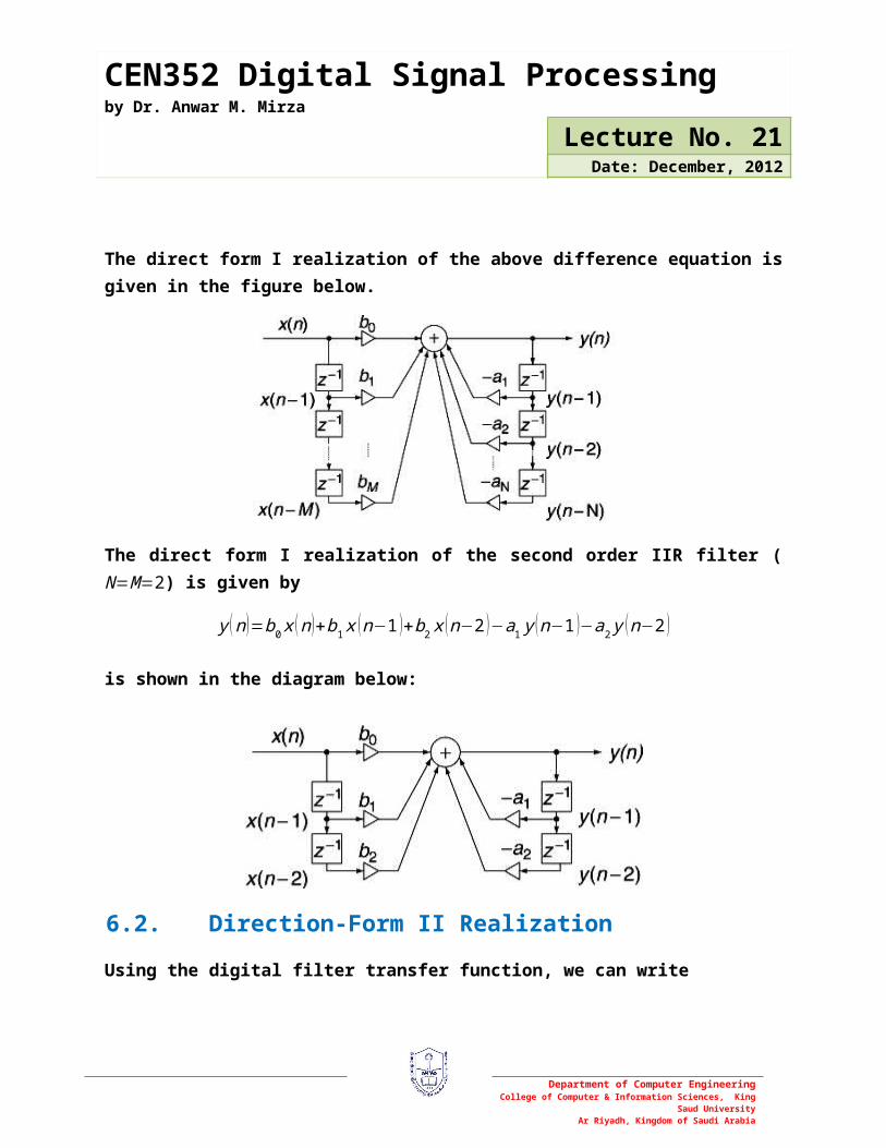
The direct form I realization of the above difference equation is given in the figure below.

Department of Computer EngineeringCollege of Computer & Information Sciences, King Saud University

Ar Riyadh, Kingdom of Saudi Arabia



The direct form I realization of the second order IIR filter (N=M=2) is given by

y (n )=b0 x (n )+b1x (n−1 )+b2x (n−2 )−a1 y (n−1 )−a2 y (n−2 )

is shown in the diagram below:

6.2. Direction-Form II Realization

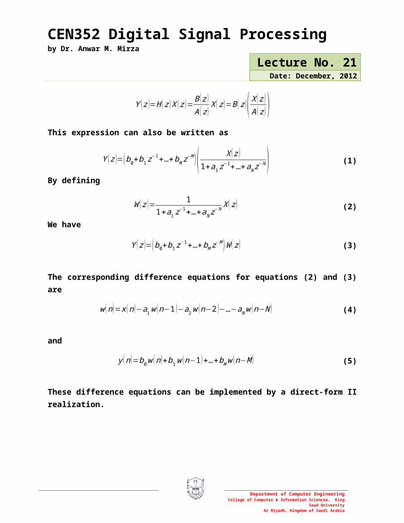
Using the digital filter transfer function, we can write

Y ( z )=H ( z )X ( z )= B ( z )A ( z )

X ( z )=B ( z )( X ( z )A ( z ) )

This expression can also be written as

Y ( z )=(b0+b1 z−1+…+bM z−M )( X ( z )

1+a1 z−1+…+aN z

−N ) (1)

By defining





W ( z )= 11+a1 z

−1+…+aN z−N X ( z ) (2)

We have

Y ( z )=(b0+b1 z−1+…+bM z−M )W ( z ) (3)

The corresponding difference equations for equations (2) and (3) are

w (n )=x (n )−a1w (n−1 )−a2w (n−2 )−…−aNw (n−N ) (4)

and

y (n )=b0w (n )+b1w (n−1 )+…+bMw (n−M ) (5)

These difference equations can be implemented by a direct-form II realization.

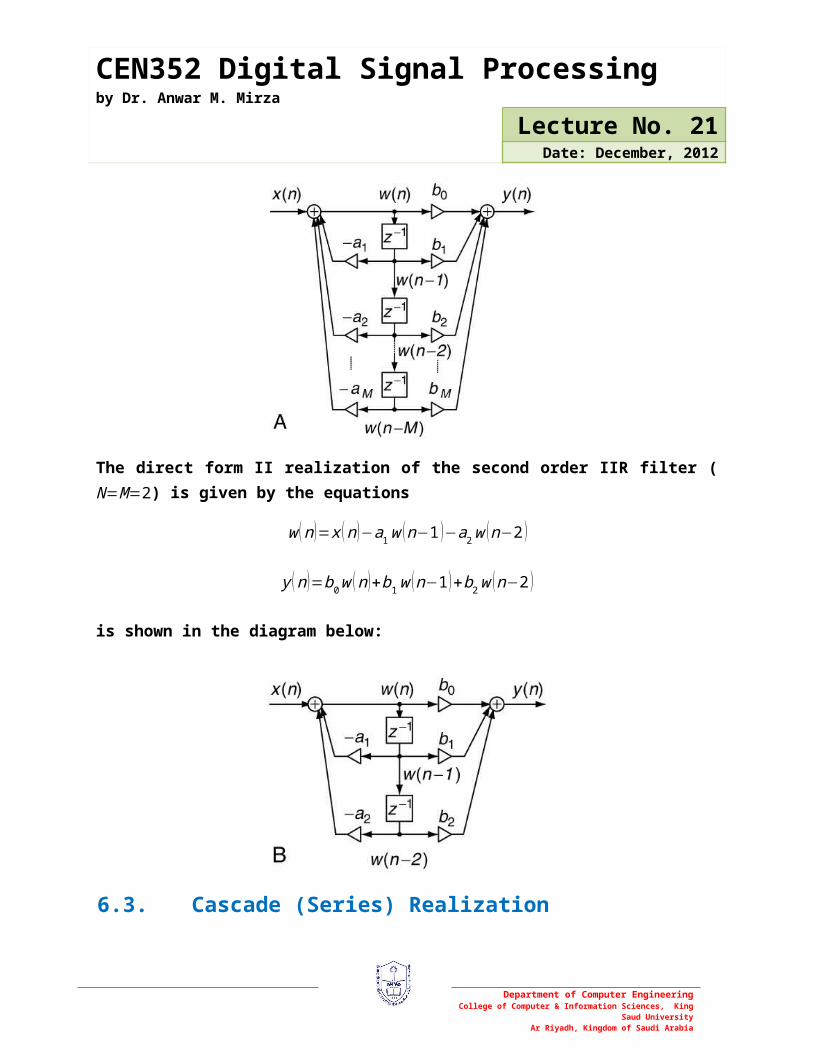
The direct form II realization of the second order IIR filter (N=M=2) is given by the equations

w (n )=x (n )−a1w (n−1 )−a2w (n−2 )





y (n )=b0w (n )+b1w (n−1 )+b2w (n−2 )

is shown in the diagram below:

6.3. Cascade (Series) Realization

The digital filter transfer function can be factorized and written as

H ( z )=H 1 ( z ) ∙H2 ( z )⋯H k ( z )

whereH k ( z ) is chosen to be first- or second-order transfer function (section), defined as,

H k ( z )=( bk 0+bk 1 z−1

1+ak1 z−1 )

Or

H k ( z )=( bk 0+bk 1 z−1+bk 2 z

−2

1+ak1 z−1+ak 2 z

−2 )The block diagram for the cascade (or series) realization is shown in figure below.

For the individual first- or second-order transfer function (section), one can use either direct form I or direct form II realizations.





6.4. Parallel Realization

The digital filter transfer function can be written as

H ( z )=H1 ( z )+H 2 ( z )+⋯+H k ( z )

whereH k ( z ) is chosen to be first- or second-order transfer function (section), defined as,

H k ( z )=( bk 0

1+ak 1 z−1 )

Or

H k ( z )=( bk 0+bk1 z−1

1+ak 1 z−1+ak2 z

−2 )The block diagram for the parallel realization is shown in figure below.

Here again, for the individual first- or second-order transfer function (section), one can use either direct form I or direct form II realizations.

Example 13

Given a second-order transfer function

H ( z )= 0.5 (1−z−1 )(1+1.3 z−1+0.36 z−2 )

Perform the filter realizations and write the difference equations using the following realizations





(1) Direct form I and direct form II(2) Cascade form via the first-order sections(3) Parallel form via the first-order sections

Solution

Part (1): The transfer function in its “delay” form can be written as

H ( z )= 0.5−0.5 z−2

1+1.3 z−1+0.36 z−2

Comparing it with the standard delay form of the transfer function

H ( z )=b0+b1 z

−1+…+bM z−M

1+a1 z−1+…+aN z

−N

We identify, thatM=1 , N=2, and

b0=0.5 , b1=0.0 ,b2=−0.5

a1=1.3 , a2=0.36

The difference equation form for the direct form I realization is given by

y (n )=0.5 x (n )−0.5 x (n−2 )−1.3 y (n−1 )−0.36 y (n−2)

The direct form I realization for this filter is shown in figure below.

For the direct form II realization, we write the difference equation as made up of the following two difference equations

w (n )=x (n )−1.3w (n−1 )−0.36w(n−2)





y (n )=0.5w (n )−0.5w (n−2 )

The direct form II realization of the filter is shown below in the figure.

Part (2): For the cascade realization, the transfer function is written in the product form. This is achieved by factorization of the numerator and the denominator polynomials. The given transfer function is

H ( z )= 0.5 (1−z−2 )1+1.3 z−1+0.36 z−2

The numerator polynomial can be factorized as

B (z )=0.5 (1−z−2 )=0.5 (1−z−1 ) (1+z−1 )

The denominator polynomial can be factorized as

A ( z )=1+1.3 z−1+0.36 z−2=1+0.4 z−1+0.9 z−1+0.36 z−2=1 (1+0.4 z−1 )+0.9 z−1 (1+0.4 z−1 )=(1+0.4 z−1 ) (1+0.9 z−1 )

Therefore, the transfer function can be written as

H ( z )= 0.5 (1−z−1 ) (1+ z−1 )(1+0.4 z−1 ) (1+0.9 z−1)

Or

H ( z )=( 0.5−0.5 z−11+0.4 z−1 )( 1+z−1

1+0.9 z−1 )=H 1 (z ) ∙H 2 ( z )

Thus, in this case





H 1 (z )=0.5−0.5 z−1

1+0.4 z−1

H 2 (z )= 1+z−1

1+0.9 z−1

Each one ofH 1 (z ) andH 2 (z ) can be realized in direct form I or direct form II. Overall, we get the cascaded realization with two sections. It should be noted that there could be other

forms forH 1 (z ) andH 2 (z ), for example, we could have taken H 1 (z )= 1+z−1

1+0.4 z−1 ,

H 2 (z )=0.5−0.5 z−1

1+0.9 z−1 , to yield the sameH ( z ). Using the former H1 (z ) andH 2 (z ), and using direct

form II realizations for the two cascaded sections, we get the following difference equations:

Section 1: (H 1 (z )=0.5−0.5 z−1

1+0.4 z−1)

w1 (n )=x (n )−0.4w (n−1 )

y1 (n )=0.5w1 (n )−0.5w1 (n−1 )

Section 2: (H 2 (z )= 1+z−1

1+0.9 z−1)

w2 (n )= y1 (n )−0.9w2 (n−1 )

y (n )=w2 (n )+w2 (n−1 )

Part (3): For the parallel realization, the transfer function is written in the partial fraction’s form. The given transfer function is

H ( z )= 0.5 (1−z−2 )1+1.3 z−1+0.36 z−2

Multiplying the numerator and denominator withz2 we get





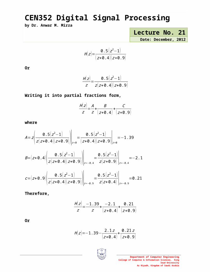
H ( z )= 0.5 ( z2−1 )z2+1.3 z+0.36

The denominator polynomial can be factorized as

A ( z )=z2+1.3 z+0.36=z2+0.4 z+0.9 z+0.36=1 ( z+0.4 )+0.9 z ( z+0.4 )= (z+0.4 ) ( z+0.9 )

Therefore, the transfer function can be written as

H ( z )= 0.5 ( z2−1 )(z+0.4 ) ( z+0.9 )

Or

H ( z )z

=0.5 ( z2−1 )

z ( z+0.4 ) ( z+0.9 )

Writing it into partial fractions form,

H ( z )z

= Az+ B

( z+0.4 )+ C

( z+0.9 )

where

A=z ( 0.5 ( z2−1 )z (z+0.4 ) ( z+0.9 ) )|z=0= 0.5 ( z2−1 )

( z+0.4 ) ( z+0.9 )|z=0=−1.39

B= ( z+0.4 )( 0.5 ( z2−1 )z ( z+0.4 ) ( z+0.9 ) )|z=−0.4

=0.5 ( z2−1 )z ( z+0.9 ) |z=−0.4

=−2.1

c= ( z+0.9 )( 0.5 ( z2−1 )z ( z+0.4 ) ( z+0.9 ) )|z=−0.9

=0.5 ( z2−1 )z ( z+0.4 ) |z=−0.9

=0.21

Therefore,

H ( z )z

=−1.39z

+ −2.1( z+0.4 )

+ 0.21( z+0.9 )

Or





H ( z )=−1.39− 2.1 z( z+0.4 )

+ 0.21 z( z+0.9 )

In delay form it can be written as

H ( z )=−1.39− 2.1(1+0.4 z−1)

+ 0.21(1+0.9 z−1 )

This can be written as

H ( z )=H 1 ( z )+H 2 ( z )+H3 ( z )

This shows that for this filter, there are three sections in the parallel realization. They can be individually realized using either direct form I or direct form II realizations. We use direct form II realization. The difference equations for each of three parallel sections are

Section 1: (H 1 (z )=−1.39)

y1 (n )=−1.39 x (n )

Section 2: (H 2 (z )= −2.1(1+0.4 z−1 ) )

w2 (n )=x (n )−0.4w2 (n−1 )

y2 (n )=2.1w2 (n )

Section 2: (H 3 ( z )= 0.21(1+0.9 z−1 ) )

w3 (n )=x (n )−0.9w3 (n−1 )

y3 (n )=−0.21w3 (n )

The output isy (n )= y1 (n )+ y2 (n )+ y3 (n ) and the parallel realization is shown below in the diagram.





Magnitude frequency response of a normalized lowpass filter.





Magnitude frequency response of a normalized highpass filter.

bandpass filter.



0

1

(a) Ideal Lowpass Frequency Response (b) Impulse Response of an Ideal Lowpass Filter



7. Finite Impulse Response (FIR) Filter Design

An FIR filter is completely specified by the following difference equation (input-output relationship):

y (n )=b0 x (n )+b1 x (n−1 )+…+bM x (n−M )=∑i=0

M

bi x (n−i ) (7.1)

The frequency response of an ideal lowpass filter is shown below in Figure (a).

bandpass filter.

Magnitude frequency response of a normalized bandreject filter.





Mathematically it is given by

H (e j Ω )={1 , 0≤|Ω|≤Ωc

0 , Ωc≤|Ω|≤π

The frequencyΩc is the lowpass cutoff frequency. It can be shown that, the corresponding impulse response of the ideal lowpass filter is as shown in Figure (b) above. A truncated part of the impulse response is shown (the actual response extends to infinity on both sides) fromn=−M ton=M . It is given by

h (n )={ Ωc

π, n=0

sin (Ωcn )πn

n≠0

The impulse response is symmetric aboutn=0. It could further be shown that, in this case the z-transform of the impulse response is given by

H ( z )=h (M ) zM+h (M−1 ) zM−1+⋯+h (1 ) z1+h (0 )+h (1 ) z−1+⋯h (M−1 ) z−M +1+h (M ) z−M

To obtain a causal impulse response, we shift (delay) the non-causal impulse response by M samples, to yield the transfer function of a causal ideal lowpass FIR filter:

H ( z )=b0+b1 z−1+b2 z

−2+⋯+b2M z−2M

where, bn=h (n−M )for n=0,1,2 ,⋯ ,2M.

Similarly, we can obtain the design equations for the other types of FIR filters, such as highpass, bandpass and bandstop. Table 7.1 gives the formulas for these FIR filters for their filter coefficient calculations.

Table 7.1: Summary of ideal impulse responses for standard FIR filtersFilter Type Ideal Impulse Response

h (n ) (non-causal FIR coefficients)Lowpass

h (n )={ Ωc

π, n=0

sin (Ωcn )πn

−M ≤n≤M





Highpass

h (n )={ π−Ωc

π, n=0

−sin (Ωcn )πn

−M ≤n≤M

Bandpass

h (n )={ ΩH−ΩL

π, n=0

sin (ΩH n )πn

−sin (ΩLn )

πn−M≤n≤M

Bandstop

h (n )={ π−ΩH+ΩL

π, n=0

−sin (ΩH n )πn

+sin (ΩL n )

πn−M≤n≤M

Causual FIR filter coefficients: shiftingh (n ) to the right by samples.Transfer Function:

H ( z )=b0+b1 z−1+b2 z

−2+⋯+b2M z−2M

Wherebn=h (n−M )for n=0,1,2 ,⋯ ,2

Example 7.2

(a) Calculate the filter coefficients for a 3-tap FIR lowpass filter with a cutoff frequency of 800 Hz and a sampling rate of 8000 Hz using the Fourier Transform method.

(b) Determine the transfer function and difference equation of the designed FIR system.(c) Compute and plot the frequency response.

Solution

Part (a): We first determine the normalized cutoff frequency

Ωc=2π f c T s=2π ×8008000

=0.2π radians

In this case2M+1=3, therefore, using table 7.1



Filter Coefficients



h (n )={ Ωc

π, n=0

sin (Ωcn )πn

−M ≤n≤ M

Therefore

h (0 )=Ωc

π=0.2π

π=0.2

h (1 )=sin (Ωc )

π=sin (0.2 π )

π=0.1871

Using symmetry, h (−1 )=h (1 )=0.1871

Delayingh (n ) byM=1 samples, we get

Part (b): Therefore, the transfer function in this case is

H ( z )=b0+b1 z−1+b2 z

−2=0.1871+0.2 z−1+0.1871 z−2

The difference equation is

y (n )=0.1871 x (n )+0.2x (n−1 )+0.1871 x (n−2 )

Part (c): The frequency response of the filter is

H (e jΩ )=0.1871+0.2e− jΩ+0.1871e−2 j Ω

It can be written as

H (e jΩ )=e− j Ω (0.1871e j Ω+0.2+0.1871 e−2 jΩ )=e− jΩ (0.2+0.1871 (e j Ω+e−2 j Ω ))=e− j Ω (0.2+0.1871×2cos (Ω ) )=e− jΩ (0.2+0.3742cos (Ω ) )

Thus, the magnitude frequency response is

|H (e jΩ )|=0.2+0.3742cos (Ω )



Linear Phase

Non-Linear Phase



And the phase response is

∠H (e jΩ )={ −Ω, 0.2+0.3742 cos (Ω )>0−Ω+π 0.2+0.3742 cos (Ω )<0

0 500 1000 1500 2000 2500 3000 3500 4000-60

-40

-20

0

Frequency (Hz)

Mag

nitu

de re

spon

se(d

B)

0 500 1000 1500 2000 2500 3000 3500 4000-150

-100

-50

0

50

100

Frequency (Hz)

Pha

se re

spon

se(d

egre

es)

Figure 7.4: Frequency response in Example 7.2

In FIR filters with symmetrical coefficients, the phase response has a linear behavior in the passband.

This means that all frequency components of the filter input within the passband are subjected to the same amount of time delay at the filter output. This is a requirement of applications in audio and speech filtering, where phase distortions needs to be avoided.

If the design method cannot produce the symmetrical coefficients, then the resultant FIR filter does not have linear phase property leading to distortions in the filtered signal. This distortion due to nonlinear phase is shown with the example below.





The FIR filter has a good phase property, but it does not give an acceptable magnitude frequency response. The result with an 17-tap lowpass filter is also shown below.

There are oscillations (ripple) in the passband (main lobe) and stopband (side lobe) of the magnitude frequency response. This is due to Gibbs oscillations, originating from the abrupt truncation of the infinite impulse response of the lowpass filter.

This behavior can be avoided with the help of windowing.





0 500 1000 1500 2000 2500 3000 3500 4000 4500-80

-60

-40

-20

0

20

Frequency (Hz)

Mag

nitu

de re

spon

se(d

B)

0 500 1000 1500 2000 2500 3000 3500 4000 4500-600

-400

-200

0

200

Frequency (Hz)

Pha

se re

spon

se(d

egre

es)

Figure 7.5: Magnitude and Phase Frequency responses of the ideal lowpass FIR filters with 3-coefficients (dashed lines) and 17 coefficients (solid lines)

Example 7.2

(a) Calculate the filter coefficients for a 5-tap FIR bandpass filter with a lower cutoff frequency of 2000 Hz and an upper cutoff frequency of 2400 at a sampling rate of 8000 Hz.

(b) Determine the transfer function and plot the frequency responses with MATLAB.

Solution



Filter Coefficients



Part (a): We first determine the normalized cutoff frequencies

ΩL=2π f Lf s

=2π × 20008000

=0.5 π radians

ΩH=2π f Hf s

=2π × 24008000

=0.6 π radians

In this case2M+1=5, therefore, from Table7.1

h (n )={ ΩH−ΩL

π, n=0

sin (ΩH n )n π

−sin (ΩLn )

n π, −2≤n≤2

The non-causal FIR coefficients are

h (0 )=ΩH−ΩL

π=0.6 π−0.5π

π=0.1

h (1 )=sin (ΩH×1 )

π×1−sin (ΩL×1 )

π ×1=sin (0.6 π )

π−sin (0.5π )

π=−0.01558

h (2 )=sin (ΩH×2 )

π×2−sin (ΩL×2 )

π ×2=sin (1.2 π )2π

−sin (1.0 π )2π

=−0.09355

Using the symmetry property

h (−1 )=h (1 )=−0.01558

h (−2 )=h (2 )=−0.09355

Thus the filter coefficients are obtained by delaying byM=2 samples, as





Part (b): Therefore, the transfer function in this case is

H ( z )=b0+b1 z−1+b2 z

−2+b3 z−3+b4 z

−4=−0.09355−0.01558 z−1+0.1 z−2−0.01558 z−3−0.09355 z−4

The difference equation is

y (n )=−0.09355 x (n )−0.01558 x (n−1 )+0.1x (n−2 )−0.01558 x (n−3 )−0.09355 x (n−4 )

Part (c): The frequency response of the filter is

H (e jΩ )=−0.09355−0.01558 e− jΩ+0.1e−2 j Ω−0.01558 e−3 jΩ−0.09355 e−4 jΩ

It can be written as

H (e jΩ )=e−2 jΩ (−0.09355 e2 jΩ−0.01558 e jΩ+0.1−0.01558 e− jΩ−0.09 355 e−2 jΩ )=e−2 jΩ (0.1−0.01558 (e jΩ+e− jΩ )−0.09355 (e2 jΩ+e−2 j Ω ))=e−2 jΩ(0.1−0.01558 (2cos (Ω ))−0.09355 (2cos (2Ω ) ) )=e−2 jΩ (0.1−0.03116cos (Ω)−0.1871 cos (2Ω ) )

Thus, the magnitude frequency response is and the phase response are computed by the MATLAB program shown below and are the plots are shown in the figure below.

[response, w] = freqz([-0.09355 -0.01558 0.1 -0.01558 -0.09355], ... [1], 512);magnitude = abs(response);magnitude2 = 20*log10(magnitude);phase2 = 180*unwrap(angle(response))/pi;figure,subplot(2,1,1); plot(w, magnitude2,'LineWidth',2); grid on;xlabel('Frequency (rad)'); ylabel('Magnitude response(dB)');subplot(2,1,2); plot(w, phase2,'LineWidth',2); grid on;xlabel('Frequency (rad)'); ylabel('Phase response(degrees)');





0 0.5 1 1.5 2 2.5 3 3.5-80

-60

-40

-20

0

Frequency (rad)

Mag

nitu

de re

spon

se(d

B)

0 0.5 1 1.5 2 2.5 3 3.50

100

200

300

Frequency (rad)

Pha

se re

spon

se(d

egre

es)

Figure 7.8: Magnitude and Phase Frequency responses of the ideal bandpass FIR filters with 5-coefficients (Example 7.3)



assignment 01 - مواقع اعضاء هيئة التدريس | ksu...

Documents