automatic physical layer tuning of mapreduce …

FEDERAL UNIVERSITY OF PARANÁ

EDSON RAMIRO LUCAS FILHO

AUTOMATIC PHYSICAL LAYER TUNING OF

MAPREDUCE-BASED QUERY PROCESSING ENGINES

CURITIBA PR - BRAZIL

2020

EDSON RAMIRO LUCAS FILHO

AUTOMATIC PHYSICAL LAYER TUNING OF

MAPREDUCE-BASED QUERY PROCESSING ENGINES

Tese apresentada como requisito parcial à obtenção

do grau de Doutor em Ciência da Computação no

Programa de Pós-Graduação em Informática, Setor de

Ciências Exatas, da Universidade Federal do Paraná.

Área de concentração: Ciência da Computação.

Orientador: Eduardo Cunha de Almeida.

CURITIBA PR - BRAZIL

2020

Catalogação na Fonte: Sistema de Bibliotecas, UFPR Biblioteca de Ciência e Tecnologia

Bibliotecária: Vanusa Maciel CRB- 9/1928

L933a Lucas Filho, Edson Ramiro

Automatic physical layer tuning of MapReduce-based query processing engines [recurso eletrônico] Edson Ramiro Lucas Filho. – Curitiba, 2020. Tese - Universidade Federal do Paraná, Setor de Ciências Exatas, Programa de Pós-Graduação em Informática, 2020.

Orientador: Eduardo Cunha de Almeida.

1. MapReduce (Computer file). 2. SQL (Linguagem de programação de computador). I. Universidade Federal do Paraná. II. Almeida, Eduardo Cunha de. III. Título.

CDD: 005.133

MINISTÉRIO DA EDUCAÇÃOSETOR DE CIENCIAS EXATASUNIVERSIDADE FEDERAL DO PARANÁPRÓ-REITORIA DE PESQUISA E PÓS-GRADUAÇÃOPROGRAMA DE PÓS-GRADUAÇÃO INFORMÁTICA -40001016034P5

TERMO DE APROVAÇÃO

Os membros da Banca Examinadora designada pelo Colegiado do Programa de Pós-Graduação em INFORMÁTICA da

Universidade Federal do Paraná foram convocados para realizar a arguição da tese de Doutorado de EDSON RAMIRO LUCAS

FILHO intitulada: Automatic Physical Layer Tuning of MapReduce-based Query Processing Engines, sob orientação do Prof.

Dr. EDUARDO CUNHA DE ALMEIDA, que após terem inquirido o aluno e realizada a avaliação do trabalho, são de parecer pela

sua APROVAÇÃO no rito de defesa.

A outorga do título de doutor está sujeita à homologação pelo colegiado, ao atendimento de todas as indicações e correções

solicitadas pela banca e ao pleno atendimento das demandas regimentais do Programa de Pós-Graduação.

CURITIBA, 29 de Junho de 2020.

Assinatura Eletrônica29/06/2020 16:23:36.0

EDUARDO CUNHA DE ALMEIDA Presidente da Banca Examinadora


STEFANIE SCHERZINGER Avaliador Externo (UNIVERSIDADE DE PASSAU - ALEMANHA)


JOSÉ MARIA DA SILVA MONTEIRO FILHO Avaliador Externo (UNIVERSIDADE FEDERAL DO CEARÁ)


LUIZ CARLOS PESSOA ALBINI Avaliador Interno (UNIVERSIDADE FEDERAL DO PARANÁ)

Rua Cel. Francisco H. dos Santos, 100 - Centro Politécnico da UFPR - CURITIBA - Paraná - BrasilCEP 81531-980 - Tel: (41) 3361-3101 - E-mail: [email protected]

Documento assinado eletronicamente de acordo com o disposto na legislação federal Decreto 8539 de 08 de outubro de 2015.Gerado e autenticado pelo SIGA-UFPR, com a seguinte identificação única: 44278

Para autenticar este documento/assinatura, acesse https://www.prppg.ufpr.br/siga/visitante/autenticacaoassinaturas.jspe insira o codigo 44278

to my wife Alessa

ACKNOWLEDGEMENTS

I would like to express my deepest appreciation to Eduardo Cunha de Almeida for all the valuable

advice during the supervision of this thesis. I’m deeply indebted to Stefanie Scherzinger for

the insightful suggestions during our collaboration in this research. I’m extremely grateful to

Herodotos Herodotou, the completion of this thesis would not have been possible without his

guidance through the Starfish’s code. I’m also grateful to Herodotos for partially funding the

experiments of this thesis. I’d also like to extend my gratitude to my friends, specially to Renato

Silva de Melo, who helped me to revise all equations. I would like to thank the National Council

for Scientific and Technological Development for the doctoral scholarship.

Agradeço aos meus pais Edson e Marilene (in memoriam) pelos ensinamentos que

me ajudaram a levar esta jornada a bom termo. Agradeço à minha esposa por todo suporte e

paciência. Agradeço ao Deus criador pelo fôlego de vida, por me habilitar, instruir e cuidar.

Futuro intangível, impossível, irrealAtrevi-me a sonhar

E não por minha forçaAqueles sofismas fez desmantelarE o irreal, impossível e intangível

Deus fez-me abundar

E nesse ímpeto caminho euPara conhecer um outro eu

Sonhado não por mim, mas por DeusCujos pensamentos são maiores do que os meus

Quais os meus não conseguem alcançar

RESUMO

A crescente necessidade de processar grandes quantidades de dados semi-estruturados e não-

estruturados levou ao desenvolvimento de mecanismos de processamento especializados como

o MapReduce. O MapReduce é um modelo de programação projetado para processar grandes

quantidades de dados semiestruturados de maneira distribuída e paralela. Os sistemas SQL-

on-Hadoop são interfaces SQL construídas sobre os mecanismos de processamento baseados

em MapReduce para consultar grandes quantidades de dados semi-estruturados. No entanto, o

número de máquinas, o número de sistemas na pilha de software e os mecanismos de controle

fornecidos pelos mecanismos do MapReduce aumentam a complexidade e os custos operacionais

de um cluster SQL-on-Hadoop. O aumento do desempenho dos motores de processamento

MapReduce é um fator chave que pode ser alcançado delegando a quantidade certa de recursos

físicos para suas tarefas. No entanto, usuários e até administradores especializados lutam

para entender e ajustar as tarefas MapReduce para obter um desempenho melhor. A falta

de conhecimento para ajustar as tarefas MapReduce deu origem a uma linha de pesquisa

bem-sucedida sobre o ajuste automático dos parâmetros do MapReduce, originando vários

Orientadores de Ajuste. No entanto, o problema de ajustar automaticamente as consultas

SQL-no-Hadoop permanece amplamente inexplorado, pois a abordagem atual da aplicação dos

Orientadores de Ajuste projetados para MapReduce em consultas SQL-on-Hadoop acarreta em

vários problemas. Por exemplo, o processador de consultas do Hive, um sistema SQL-on-Hadoop

popular, traduz consultas HiveQL em grafos de tarefas MapReduce, e seria fácil supor que,

ajustando as configurações do motor de processamento MapReduce, as consultas HiveQL também

se beneficiariam. Entretanto, essa suposição não se aplica quando os Orientadores de Ajuste

existentes são aplicados ingenuamente às consultas HiveQL devido a arquitetura do Hive, Hadoop

e dos Orientadores de Ajuste. Nesta tese tratamos da questão de como ajustar corretamente as

consultas SQL-no-Hadoop. Por “corretamente”, entendemos que, ao ajustar as configurações das

consultas SQL-no-Hadoop, a geração das configurações deve considerar várias características que

estão presentes apenas em tarefas geradas pelos sistemas SQL-no-Hadoop. Essas características

incluem: (i) no caso de consultas individuais, todas as tarefas MapReduce que constituem o

plano de consulta desta consulta são executadas com configurações idênticas. (ii) apesar da busca

e geração das configurações de ajuste serem realizadas para cada tarefa MapReduce, apenas uma

configuração de ajuste é selecionada e aplicada à consulta e as demais configurações de ajuste

são simplesmente descartadas. (iii) Os Orientadores de Ajuste do Hadoop tratam as funções do

MapReduce como caixas-pretas e fazem suposições de modelagem simplificadoras que podem

valer para tarefas clássicas do MapReduce (Sort, Grep), mas não são verdadeiras para consultas

do tipo SQL como o HiveQL, onde as tarefas contêm vários operadores de álgebra relacional

como junções e agregadores. Estendemos o processador de consultas do Hive para ajustar

as consultas SQL-no-Hadoop. Esta extensão compreende uma abordagem chamada de ajuste

não-uniforme que permite que os sistemas SQL-on-Hadoop tenham um controle mais refinado da

configuração das consultas, onde cada tarefa MapReduce recebe uma configuração especializada.

Apresentamos um modelo conceitual, chamado assinatura de código, que usa informações

estáticas disponíveis antes da execução de cada tafera para mapear tarefas que tenham padrões de

consumo de recursos similares. Também apresentamos um cache que armazena configurações de

ajuste, geradas por algum Orientadore de Ajuste, e as recicla entre tarefas que possuem consumo

de recursos semelhantes. Nossa extensão funciona em conjunto como uma solução única para

o ajuste automático de consultas SQL-no-Hadoop. Para validar nossa solução, realizamos um

estudo experimental focado no Hive executando sobre o Hadoop porque (i) O Hive é um bom

representante dos sistemas SQL-on-Hadoop nativos (como o System-R fez para os sistemas de

bancos de dados relacionais); (ii) o Hive e o Hadoop são altamente populares para processamento

analítico; e (iii) O ajuste de parâmetros do Hadoop foi estudado extensivamente nos últimos

anos. Para preencher o cache de ajuste, empregamos o Starfish, o primeiro Orientador de Ajuste

baseado em custo que encontra configurações (quase) ótimas e é o único Orientador de Ajuste

disponível ao público para fins de pesquisa acadêmica. Em nossos experimentos, apresentamos

que as consultas otimizadas com nossa abordagem de ajuste apresentaram acelerações de até

25%, contrastando com a abordagem atual que degradou o desempenho em várias ocasiões.

Especificamente, a abordagem atual de ajuste pode causar variações no tempo de execução

entre -171% e 27% em relação à configuração padrão. Mais importante ainda, nosso método

de ajuste leva a uma melhor utilização de recursos, diminuindo o uso da CPU e a paginação de

memória em até 40%. Nossa abordagem também reduziu a quantidade total de dados gravados

em discos em 5×. Nossa abordagem de ajuste tem um cache usado para evitar a recriação de

perfis de tarefas MapReduce semelhantes. Nosso cache reduziu a geração de perfils em 50%

para a carga de trabalho TPC-H, permitindo até o ajuste parcial de consultas ad-hoc antes de

sua execução. Palavras-chave: Sintonia da camada física. Processamento de consulta em

MapReduce. SQL-On-Hadoop.

ABSTRACT

The increasing need to process large amounts of semi- and non-structured data has led to the

development of specialized processing engines like MapReduce. MapReduce is a programming

model designed to process large-scale semi-structured data in a distributed and parallel fashion.

SQL-on-Hadoop systems are SQL-like interfaces build on top of MapReduce processing engines

to query semi-structured data in large-scale. However, the number of computing nodes, the

number of systems in the software stack, and the controlling mechanisms provided by MapReduce

engines increase the complexity and the operational costs of maintaining a large SQL-on-Hadoop

cluster. Increasing performance of such engines is a key factor that can be achieved by delegating

the right amount of physical resources. Yet, regular users and even expert administrators struggle

to understand and tune MapReduce jobs to achieve good performance. This skill gap has

given rise to a successful line of research on automatically tuning MapReduce parameters,

originating several tuning advisors. Yet, the problem of automatically tuning SQL-on-Hadoop

queries remains largely unexplored today as the current approach of applying MapReduce tuning

advisors direct to SQL-on-Hadoop queries entail a number of problems. For instance, the

Hive SQL-on-Hadoop engine compiles HiveQL queries into a workflow of MapReduce jobs,

and it would be straightforward to assume that by tuning the underlying Hadoop processing

engine, HiveQL queries would benefit as well. However, this assumption does not hold when

existing tuning advisors are naively applied to HiveQL queries due to the design choices of Hive,

Hadoop, and the tuning advisors. This thesis addresses the question of how to properly tune

SQL-on-Hadoop queries? By “properly” we mean, when tuning SQL-on-Hadoop queries, the

generation of the tuning setups has to consider several characteristics that are only present in

jobs generated by SQL-on-Hadoop systems. These characteristics include: (i) at the level of

individual queries, all MapReduce jobs that constitute a query plan are executed with identical

configuration settings. (ii) despite profiling and search heuristics being performed in a job-basis

to generate tuning setups, only one tuning setup is applied to the query and the remaining tuning

setups are simply discarded. (iii) Hadoop tuning advisors treat the MapReduce functions as black

boxes and make simplifying modeling assumptions that may hold for classical MapReduce jobs

(Sort, Grep), but they are not true for SQL-like queries like HiveQL where jobs contain multiple

relational algebra operators like joins and aggregators. We extended the Hive query processor for

tune SQL-on-Hadoop queries. This extension comprises an approach called non-uniform tuning

that enables SQL-on-Hadoop systems to have a fine-grained control for tuning queries, where

jobs receive specialized tuning setups. We present a conceptual model, called code-signature,

that uses static information available upfront execution to match jobs with similar resource

consumption patterns. We also present a tuning cache that stores tuning setups, generated by third

part tuning advisors, and recycle them between jobs that have the similar resource consumption.

The extension works together as a single solution for automatic tuning of SQL-on-Hadoop queries.

In order to validate our solution, we conduct an experimental study focused on Hive over Hadoop

because (i) Hive is a good representative of native SQL-on-Hadoop systems (like System-R did

for relational database systems); (ii) both Hive and Hadoop are highly popular for analytical

processing; and (iii) Hadoop parameter tuning has been studied extensively in recent years.

For populate the Tuning Cache, we employ Starfish, the first cost-based optimizer for finding

(near-) optimal configuration parameter settings and the only publicly available tuning advisor

for academic research purposes. In our experiments, we present that queries optimized with our

tuning approach always presented positive speed ups up to 25%, contrasting the current approach

that degraded performance in several occasions. Specifically, the current tuning approach can

cause variations in the execution run time between -171% and 27% over default configuration.

Most importantly, our tuning method leads to considerable better resource utilization, decreasing

CPU usage and Memory paging over 40%. Also reducing the total amount of data written to

disks in 5×. Our tuning approach has a Tuning Cache used to avoid reprofiling similar jobs. Our

Tuning Cache reduced the profilings in 50% for TPC-H queries, enabling upfront tuning of ad-hoc

queries. Keywords: Physical-layer tuning. MapReduce query processing. SQL-On-Hadoop.

LIST OF FIGURES

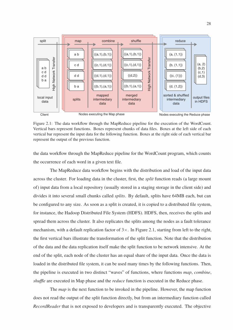
2.1 The data workflow through the MapReduce pipeline for the execution of the

WordCount. Vertical bars represent functions. Boxes represent chunks of data

files. Boxes at the left side of each vertical bar represent the input data for the

following function. Boxes at the right side of each vertical bar represent the

output of the previous function. . . . . . . . . . . . . . . . . . . . . . . . . . 28

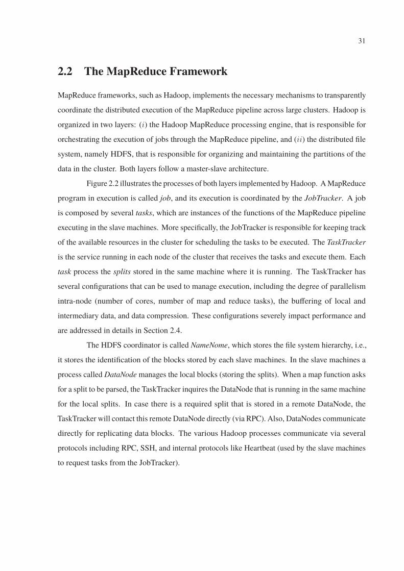
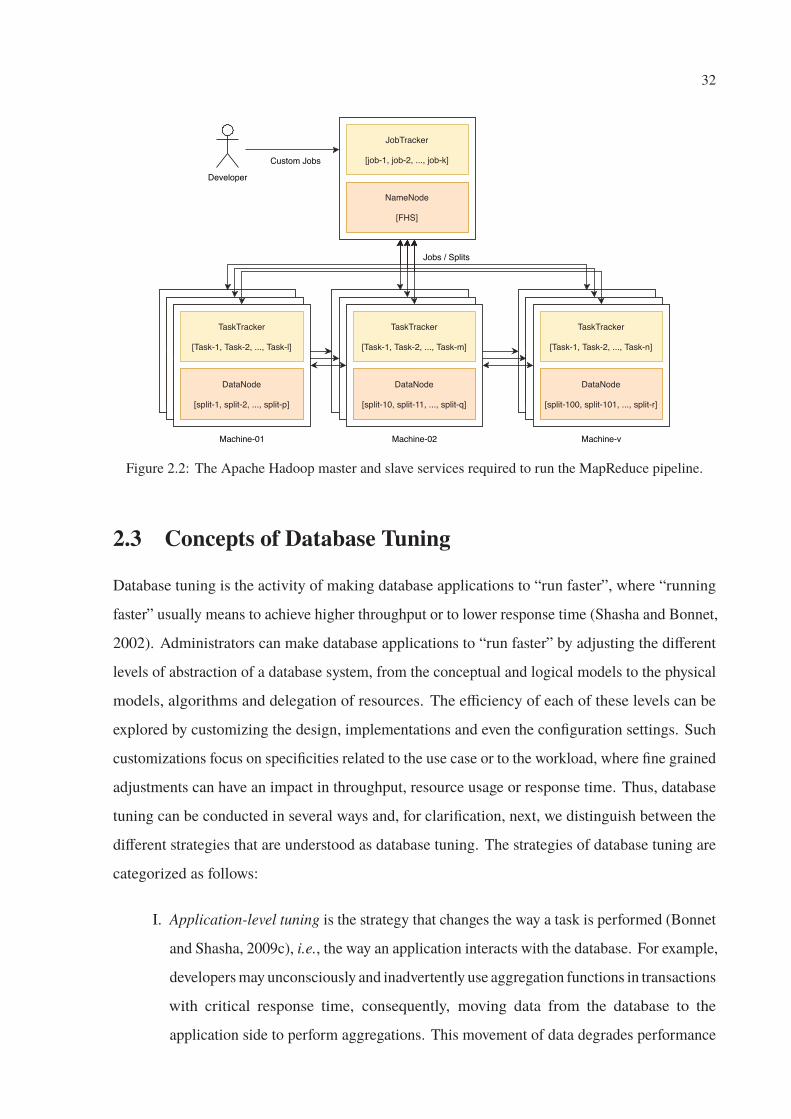
2.2 The Apache Hadoop master and slave services required to run the MapReduce

pipeline. . . . . . . . . . . . . . . . . . . . . . . . . . . . . . . . . . . . . . . 32

2.3 Number of tuning parameters growing over system releases 1. These values were

obtained from the configuration files or the source code. . . . . . . . . . . . . 36

2.4 Hive query plan for TPC-H query 7. . . . . . . . . . . . . . . . . . . . . . . . 47

2.5 (a) Uniform and (b) Non-Uniform tuning workflow. . . . . . . . . . . . . . . . 48

3.1 Query plans for TPC-H query 7. . . . . . . . . . . . . . . . . . . . . . . . . . 52

3.2 Speedups of TPC-H queries achieved by uniform tuning (in %) for each candidate

tuning setup. The tuning setups generated for the dominant job (in terms of run

time) are marked by ∗. . . . . . . . . . . . . . . . . . . . . . . . . . . . . . . 58

3.3 Maximum, average, and minimum speedup of uniform tuning (using Option 2)

for queries with 1, 2, or more dominant (i.e., long running) jobs within the same

query plan. . . . . . . . . . . . . . . . . . . . . . . . . . . . . . . . . . . . . 62

3.4 The execution breakdown of jobs in the query run time (run with default

configuration). Right: Percentage of the dominant job(s) in the query execution

time. Jobs are classified into cases A–C, depending on their share of query runtime. 63

4.1 Speedup of uniform and non-uniform tuning approaches relative to the default

configuration. . . . . . . . . . . . . . . . . . . . . . . . . . . . . . . . . . . . 70

4.2 The accumulated resource consumption percentage of uniform and non-uniform

tuning relative to the default configuration (baseline). Less is better. . . . . . . 72

4.3 Distribution of execution times of the reduce tasks for each tuning approach. . . 73

4.4 The total amount of data written to the local and distributed file system during

the shuffle and reduce phase of the 22 TPC-H queries. . . . . . . . . . . . . . . 75

4.5 Average resource consumption of the 10 machines of the cluster during a single

execution of TPC-H query 7. Solid black lines indicate the beginning of each of

the 6 jobs in the query plan, and dashed black lines indicate the end of query

execution. . . . . . . . . . . . . . . . . . . . . . . . . . . . . . . . . . . . . . 76

5.1 Execution of selected TPC-H queries. The jobs labeled 1’ share the same code

signature and apparently have similar resource profiles. This suggests that they

would benefit from the same tuning setup. . . . . . . . . . . . . . . . . . . . . 81

5.2 The architecture of the extension made in the Hive query processing engine.

Illustration of the lookups in the code signature cache. For a cache miss, a

third-party tuning adviser is run to generate a tuning setups. . . . . . . . . . . . 84

5.3 MapReduce jobs compiled from TPC-H queries: Counting jobs that share the

same code signature. Executing in Hive 0.6.0 and Hadoop 0.20.0 . . . . . . . . 86

5.4 MapReduce jobs compiled from TPC-H queries: Counting jobs that share the

same code signature. Executing in Hive 3.0 and Hadoop 2.0. . . . . . . . . . . 86

5.5 MapReduce jobs compiled from TPC-DS queries: Counting jobs that share the

same code signature. Executing in Hive 3.0 and Hadoop 2.0. . . . . . . . . . . 87

5.6 Jobs with the same code signature tend to benefit from the same tuning setups.

This effect cannot be repeated for jobs with different code signatures. . . . . . . 88

5.7 Execution run time of jobs running with tuning setups generated for jobs with

same and different code-signatures. Low standard deviation means that reusing

tuning setups from jobs that shares the same code-signature will produce similar

execution run times. But, the standard deviation is high when using tuning setups

from jobs with different code-signatures, because reusing tuning setups from

jobs with different code-signatures produces different impact on performance. . 88

5.8 The Tuning Cache reduces the profiling time by over 50% for TPC-H. . . . . . 90

5.9 Accumulated time for profiling all queries. . . . . . . . . . . . . . . . . . . . . 91

5.10 Accumulated time for profiling. Varying the order in query profiling. . . . . . . 91

A.1 Resource Consumption of TPC-H query 1 executing with default configuration. 111






















LIST OF TABLES

2.1 Hadoop tuning advisers and the supported tuning parameters. Note that the old

and new names of the tuning parameters are listed together. Tuning advisers with

�symbol use the new names of the tuning parameter. Tuning advisers without

symbol use the old names of the tuning parameters. . . . . . . . . . . . . . . . 37

2.2 Spark tuning advisers and the supported tuning parameters. . . . . . . . . . . . 38

2.3 Hadoop tuning advisers, ordered by year of publication. Listing reported speed

up, Hadoop version supported, and heuristics employed. ∗SPSA: Simultaneous

Perturbation Stochastic Approximation. . . . . . . . . . . . . . . . . . . . . . 41

2.4 Spark tuning advisers, ordered by year of publication. Listing reported speed up,

supported version, and the heuristic employed. . . . . . . . . . . . . . . . . . . 42

2.5 Benchmarks employed by Hadoop tuning advisers. . . . . . . . . . . . . . . . 43

2.6 Benchmarks employed by Spark tuning advisers. . . . . . . . . . . . . . . . . 44

3.1 TPC-H queries with their HiveQL Operators (aggregated), number of MapReduce

jobs, number of Map and Reduce tasks, input data size, and run time in our

execution environment. For more details about the occurrence of each operator

per job, see Appendix B. . . . . . . . . . . . . . . . . . . . . . . . . . . . . . 55

3.2 Selected parameter values generated by Starfish for each job of TPC-H query 7

and the default (out-of-the-box) tuning values shown on the right. (∗Job-1 is a

map-only job; hence, mapred.reduce.tasks is not set. †By default, Hive

overrides mapred.reduce.task based on the input size of each job.) . . . 56

3.3 Selected parameter values for each MapReduce job of TPC-H queries 1-11. . . 59

3.4 Selected parameter values for each MapReduce job of TPC-H queries 12-22. . . 60

4.1 Average run time (in seconds) per job of query 7 running with the default

configuration, non-uniform, and uniform tuning. . . . . . . . . . . . . . . . . . 77

B.1 Occurrence of operators per job of TPC-H query 1. . . . . . . . . . . . . . . . 123









B.10 Occurrence of operators per job of TPC-H query 10. . . . . . . . . . . . . . . 125













TABLE OF CONTENTS

1 Introduction 17

1.1 Problem Statement . . . . . . . . . . . . . . . . . . . . . . . . . . . . . . . . 20

1.2 Research Question . . . . . . . . . . . . . . . . . . . . . . . . . . . . . . . . 23

1.3 Motivation . . . . . . . . . . . . . . . . . . . . . . . . . . . . . . . . . . . . . 24

1.4 Contributions . . . . . . . . . . . . . . . . . . . . . . . . . . . . . . . . . . . 25

1.5 List of Publications . . . . . . . . . . . . . . . . . . . . . . . . . . . . . . . . 26

1.6 Document Structure . . . . . . . . . . . . . . . . . . . . . . . . . . . . . . . . 26

2 Theoretical Foundation & Related Work 27

2.1 The MapReduce Programming Model . . . . . . . . . . . . . . . . . . . . . . 27

2.2 The MapReduce Framework . . . . . . . . . . . . . . . . . . . . . . . . . . . 31

2.3 Concepts of Database Tuning . . . . . . . . . . . . . . . . . . . . . . . . . . . 32

2.4 Tuning Advisors for Hadoop (Related Work) . . . . . . . . . . . . . . . . . . . 34

2.4.1 Configuration parameters . . . . . . . . . . . . . . . . . . . . . . . . . 34

2.4.2 Profiling the job resource usage . . . . . . . . . . . . . . . . . . . . . 39

2.4.3 Searching for the (near-) optimal tuning setup . . . . . . . . . . . . . . 39

2.5 Query Execution in Hive . . . . . . . . . . . . . . . . . . . . . . . . . . . . . 45

2.6 Parameter Tuning in Hive . . . . . . . . . . . . . . . . . . . . . . . . . . . . . 47

3 Tuning SQL-on-Hadoop Systems 50

3.1 The SQL-on-Hadoop Tuning Problem . . . . . . . . . . . . . . . . . . . . . . 50

3.2 The Uniform Tuning Approach . . . . . . . . . . . . . . . . . . . . . . . . . . 53

3.2.1 Experiment Setup . . . . . . . . . . . . . . . . . . . . . . . . . . . . . 54

3.2.2 Experimental Methodology . . . . . . . . . . . . . . . . . . . . . . . 55

3.2.3 Performance of Candidate Tuning Setups . . . . . . . . . . . . . . . . 56

3.2.4 Strategies for Selecting a Tuning Setup . . . . . . . . . . . . . . . . . 61

3.3 Discussion . . . . . . . . . . . . . . . . . . . . . . . . . . . . . . . . . . . . . 64

4 Intra-Query Physical-Layer Tuning 65

4.1 The Non-Uniform Tuning Approach . . . . . . . . . . . . . . . . . . . . . . . 65

4.2 Performance of Non-Uniform Tuning . . . . . . . . . . . . . . . . . . . . . . . 66

4.3 Cost of the Non-Uniform Tuning . . . . . . . . . . . . . . . . . . . . . . . . . 67

4.4 Non-Uniform Tuning Methodology . . . . . . . . . . . . . . . . . . . . . . . . 68

4.5 Performance of Uniform vs. Non-Uniform Tuning . . . . . . . . . . . . . . . . 69

4.6 Impact on Resource Utilization . . . . . . . . . . . . . . . . . . . . . . . . . . 71

4.6.1 Resource Utilization of Uniform vs. Non-uniform Tuning . . . . . . . . 71

4.6.2 In-Depth Analysis for Query 7 . . . . . . . . . . . . . . . . . . . . . . 74

4.7 Discussion . . . . . . . . . . . . . . . . . . . . . . . . . . . . . . . . . . . . . 77

5 Recycling Tuning Setups 79

5.1 The Tuning Cache . . . . . . . . . . . . . . . . . . . . . . . . . . . . . . . . . 80

5.1.1 Code Signatures . . . . . . . . . . . . . . . . . . . . . . . . . . . . . 80

5.1.2 Code Signature Definition . . . . . . . . . . . . . . . . . . . . . . . . 82

5.1.3 Architecture of the Tuning Cache . . . . . . . . . . . . . . . . . . . . 83

5.2 Recycling Tuning Setups at the Job Level . . . . . . . . . . . . . . . . . . . . 85

5.2.1 Repeating Code-Signatures . . . . . . . . . . . . . . . . . . . . . . . . 85

5.2.2 Justifying the Recycling of Tuning Setups . . . . . . . . . . . . . . . . 87

5.3 Recycling Tuning Setups at the Query Level . . . . . . . . . . . . . . . . . . . 89

5.3.1 Profiling the TPC-H Queries in Order . . . . . . . . . . . . . . . . . . 89

5.3.2 Recycling vs. Starfish Sampling . . . . . . . . . . . . . . . . . . . . . 90

5.3.3 Varying the Query Order . . . . . . . . . . . . . . . . . . . . . . . . . 91

5.4 Discussion . . . . . . . . . . . . . . . . . . . . . . . . . . . . . . . . . . . . . 92

6 Conclusion 93

6.1 Lessons Learned . . . . . . . . . . . . . . . . . . . . . . . . . . . . . . . . . 93

6.2 Future Work . . . . . . . . . . . . . . . . . . . . . . . . . . . . . . . . . . . . 96

APPENDIX A – RESOURCE CONSUMPTION OF TPC-H QUERIES 110

APPENDIX B – OCCURRENCE OF OPERATORS IN TPC-H QUERIES 122

17

Chapter 1

Introduction

The progress of computer technology simplified many daily activities in wide aspects, such

as, connecting people despite their distances, bringing customers to stores without taken them

out of home, and providing a large variety of tailor made services that ranges from movie

recommendations to directed product advertisements. The facilities provided by such applications

come at the cost of generating, storing and processing large amounts of data. Traditionally, raw

data is extracted from one or many sources and, then, transformations such as data cleaning, and

filtering are performed. After the data is harvested and standardized with such transformations, it

is loaded in a database system for later querying. Data Warehouse systems have been extensively

employed in such scenario, also known as the extract-transform-load (ETL) data workflow.

In ETL, data is prepared upfront querying, therefore, the set of transformations must be

performed for every new batch of data. More specifically, data have to be stored in a staging

area, and then, costly transformations like cleaning, filtering and aggregations are performed.

ETL is the most common method for loading large data into database systems. It guarantees

that all data is stored following a trustworthy, concise and structured way. Yet, data might be

produced at such a high pace that the extraction and transformations become overloaded and hard

to manage. Examples include web logs, radio-frequency identification tags, sensor networks, and

social networks (Vaisman and Zimnyi, 2016). One of the solutions for this problem is to provide

the data warehouse capabilities directly on raw non-structured and semi-structured data sets, or

to provide processing engines that are capable of scaling out such transformations according to

the pace of data production.

The increasing need to process large amounts of semi- and non-structured data has led to

the development of specialized processing engines like MapReduce (Dean and Ghemawat, 2004).

18

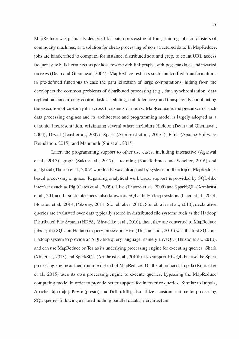
MapReduce was primarily designed for batch processing of long-running jobs on clusters of

commodity machines, as a solution for cheap processing of non-structured data. In MapReduce,

jobs are handcrafted to compute, for instance, distributed sort and grep, to count URL access

frequency, to build term-vectors per host, reverse web-link graphs, web-page rankings, and inverted

indexes (Dean and Ghemawat, 2004). MapReduce restricts such handcrafted transformations

in pre-defined functions to ease the parallelization of large computations, hiding from the

developers the common problems of distributed processing (e.g., data synchronization, data

replication, concurrency control, task scheduling, fault tolerance), and transparently coordinating

the execution of custom jobs across thousands of nodes. MapReduce is the precursor of such

data processing engines and its architecture and programming model is largely adopted as a

canonical representation, originating several others including Hadoop (Dean and Ghemawat,

2004), Dryad (Isard et al., 2007), Spark (Armbrust et al., 2015a), Flink (Apache Software

Foundation, 2015), and Mammoth (Shi et al., 2015).

Later, the programming support to other use cases, including interactive (Agarwal

et al., 2013), graph (Sakr et al., 2017), streaming (Katsifodimos and Schelter, 2016) and

analytical (Thusoo et al., 2009) workloads, was introduced by systems built on top of MapReduce-

based processing engines. Regarding analytical workloads, support is provided by SQL-like

interfaces such as Pig (Gates et al., 2009), Hive (Thusoo et al., 2009) and SparkSQL (Armbrust

et al., 2015a). In such interfaces, also known as SQL-On-Hadoop systems (Chen et al., 2014;

Floratou et al., 2014; Pokorny, 2011; Stonebraker, 2010; Stonebraker et al., 2010), declarative

queries are evaluated over data typically stored in distributed file systems such as the Hadoop

Distributed File System (HDFS) (Shvachko et al., 2010), then, they are converted to MapReduce

jobs by the SQL-on-Hadoop’s query processor. Hive (Thusoo et al., 2010) was the first SQL-on-

Hadoop system to provide an SQL-like query language, namely HiveQL (Thusoo et al., 2010),

and can use MapReduce or Tez as its underlying processing engine for executing queries. Shark

(Xin et al., 2013) and SparkSQL (Armbrust et al., 2015b) also support HiveQL but use the Spark

processing engine as their runtime instead of MapReduce. On the other hand, Impala (Kornacker

et al., 2015) uses its own processing engine to execute queries, bypassing the MapReduce

computing model in order to provide better support for interactive queries. Similar to Impala,

Apache Tajo (tajo), Presto (presto), and Drill (drill), also utilize a custom runtime for processing

SQL queries following a shared-nothing parallel database architecture.

19

Facebook reports that their Hive data warehouse stores more than 15PB of data and

loads more than 60TB of new data every day (Menon, 2012; Thusoo et al., 2009; Thusoo et al.,

2010). All this data is stored in the Hadoop processing engine, more specifically, in its underlying

distributed file system (HDFS), and both run together over thousands of machines (Borthakur et al.,

2011). Compression is applied to reduce the amount of stored data (with reported compression

ratio of 1:7). However, the amount of stored data is usually increased by a factor of 3× or more

because HDFS uses data replication as a fail-over mechanism. The replication of the data, together

with other internal controlling mechanisms (that hide from developers the problems of processing

such distributed queries, e.g., concurrency control, task scheduling, data synchronization) inflict

such an impact in the operational costs of maintaining a large SQL-on-Hadoop cluster as well

as in the performance of the MapReduce processing engines (Ciritoglu et al., 2018; Zaharia

et al., 2008). In this scenario, performance can be understood in terms of execution run time as

well as in terms of resource consumption. Thus, deploying SQL-on-Hadoop systems to execute

distributed queries over large amounts of data is advantageous because it widely facilitates and

simplifies the daily activities of database administrators and data scientists. Yet, it comes at high

operational costs due to the number of computing resources (e.g, disk, network) required to

provide a reliable framework to run such distributed queries.

Increasing performance is a key driving factor that can be achieved by delegating the

right amount of physical resources to jobs (e.g., memory size, number of cores). The performance

of the underlying processing engines (such as MapReduce and Spark) and custom runtimes (e.g.,

of Impala, Tajo) is governed via a large number of configuration parameters that control memory

distribution, I/O optimization, task parallelism, and data compression (Herodotou et al., 2011;

Ding et al., 2015; Bei et al., 2017). For example, both MapReduce and Spark have over 200

parameters each, out of which 20-40 can have significant impact on the performance and stability

of the cluster. Several studies have shown that MapReduce jobs can experience up to an order of

magnitude difference in execution time between good and bad parameter settings (Babu, 2010;

Jiang et al., 2010).

However, regular users and even expert administrators struggle to understand and tune

them to achieve good performance. A recent report highlights that the proliferation of MapReduce

goes hand-in-hand with continuous lamentations regarding the lack of professionals who can tune

a Hadoop cluster (Heudecker and Adrian, 2015). This skills gap has given rise to a successful

line of research on automatically tuning MapReduce and Spark parameters, originating several

20

tuning advisors that employ a variety of techniques such as cost models, simulation, and machine

learning (Liu et al., 2015; Liao et al., 2013; Shi et al., 2014; Liu et al., 2012; Bei et al., 2016;

Li et al., 2014b; Bei et al., 2017; Van Aken et al., 2017; Herodotou et al., 2011, 2020). These

tuning advisors are designed specially for tuning common MapReduce workloads (Sort, Grep,

WordCount). However, employing them straightforwardly to SQL-on-Hadoop queries entails a

number of problems.

Shared-nothing parallel database systems support a vast set of multi-tenant workloads,

yet, no configuration tuning approach works well universally (Abadi et al., 2020). This thesis

presents a set of techniques and mechanisms to overcome the problems that arise when applying

MapReduce tuning advisors to tune SQL-on-Hadoop queries. We focus on physical-layer tuning

of SQL-on-Hadoop queries, i.e., the allocation of the right amount of physical resources (i.e.,

memory, cores, bandwidth) to queries in order to reduce the execution costs (i.e., running time,

resource usage). For example, in MapReduce, regulating the size of memory buffers leads queries

to spill less data into disk, consequently, making less disk operations; also, increasing the number

of threads may speed up queries by increasing the degree of parallelism.

We conduct an experimental study focused on Hive over Hadoop because (i) Hive

is a good representative of native SQL-on-Hadoop systems (like System-R did for relational

database systems); (ii) both Hive and Hadoop are highly popular for analytical processing; and

(iii) Hadoop parameter tuning has been studied extensively in recent years (Khaleel, 2018; Cai

et al., 2017; Deshpande et al., 2018; Khan et al., 2017; Kumar et al., 2017; Jain, 2017; Bei et al.,

2017; Lee and Fortes, 2016; Zhang et al., 2016). We explore the impact of Hadoop parameter

tuning on Hive, identify the potential use of existing Hadoop tuning advisors for optimizing Hive

performance, and propose a set of mechanisms for parameter tuning of SQL-on-Hadoop systems.

For tuning Hadoop, we employ Starfish (Herodotou et al., 2011; Herodotou and Babu, 2011), the

first cost-based optimizer for finding (near-) optimal configuration parameter settings and the

only publicly available tuning advisor for academic research purposes.

1.1 Problem Statement

MapReduce-based processing engines expose a vast number of configuration parameters that

regulate the amount of physical resources given to jobs. Such configuration parameters highly

influences the performance of the jobs (good parameter settings are proven to speed up execution

21

up to an order of magnitude (Babu, 2010; Jiang et al., 2010)). When submitting a MapReduce

job, administrators can configure it by hard-coding its configuration in the source code, or

instrumenting it via command line. In both cases, the configuration parameters are set in a job

basis, where jobs have different configuration settings according to their requirements. Note,

the optimal amount of resources required by each job differs because they process different

operations over different data sets.

These settings can be configured not only by administrators, which are the deep

connoisseurs of the infrastructure and the most recommended experts to determine the tuning

values, but also by developers, who might be greedy in delegating resources expecting that their

jobs finish as soon as possible. However, since finding the optimal tuning setup for a single job is

time consuming and error prone, MapReduce processing engines delegate the tuning activity to

tuning advisors. Several MapReduce tuning advisors calculate the (near-) optimal configuration

settings at the cost of a high overhead due to the requirements for calculating such tuning setups.

A MapReduce tuning advisor monitors a test-run of the job to measure its resource

consumption, generating a representation called execution profile. Given an execution profile,

the tuning advisor employs a modeling technique (e.g., cost or analytical modeling, machine

learning, simulation) to estimate the execution time of the given job under a given tuning setup

(Glushkova et al., 2019; Zhang et al., 2013a; Song et al., 2013; Cherkasova, 2011). These models

commonly represent the environment where jobs are executed, more specifically, the underlying

processing engine and hardware, which makes tuning advisors very attached to specific software

versions. Then, the tuning advisor enumerates and search over the high-dimensional space of

parameter values in order to identify the tuning setup that will produce the smallest execution

time. Different advisors will employ different search strategies, ranging from grid search and

exhaustive enumeration to hill climbing and genetic algorithms.

Similar to tuning a MapReduce job, a Hive administrator can tune a HiveQL statement

by assigning the tuning setup in the query code, or when submitting the query via Hive command

line. However, the generation of the tuning setup and its impact in the performance of the HiveQL

query is influenced by several aspects that are only present in jobs generated by SQL-on-Hadoop

systems . For instance, Hive translates a given HiveQL statement to a workflow of MapReduce

jobs to be executed on Hadoop or Tez. Precisely, a HiveQL statement is parsed and validated

against the data dictionary, compiled into a tree of logical operators, and finally optimized

to produce a physical query execution plan (Floratou et al., 2014; Thusoo et al., 2010). This

22

allows for various logical optimizations such as selection and projection pushdowns, as well as

join reordering and join physical method selection. The final execution plan has the form of a

Directed Acyclic Graph (DAG) of MapReduce jobs, where each job is executed on the cluster

as a set of parallel Map and Reduce tasks. During the generation of the final execution plan,

Hive replicates the given tuning setup to all jobs in the query plan, i.e., at the level of individual

HiveQL queries, all MapReduce jobs that constitute a query plan are executed with identical

configuration settings.

The replication of the same configuration settings to all jobs in the query plan restricts

the tuning to a query-level and forbid developers and administrators to tune jobs of the same

query plan separately. Hence, when administrators are tasked with tuning a query, they must

find a single setting of parameter values to use on a per-query basis, or even for the complete

query workload. Even with the help of a MapReduce tuning advisor, the same tuning setup will

still be replicated to the entire query plan, driving SQL-on-Hadoop queries to under-perform.

For instance, a job may need a tuning setup for disk intensive sequential scan operations, but it

receives a tuning generated for a job with memory bound sort operations (see Chapter 5).

When MapReduce tuning advisors are applied for tuning SQL-on-Hadoop queries, they

generate tuning setups in a job basis, i.e., MapReduce tuning advisors will profile and run search

heuristics to find the (near-) optimal tuning setup for every job in the query plan. Yet, only

one tuning setup is selected for tuning the query, and the remaining tuning setups are simply

discarded. In this case, an important amount of time is wasted for generating tuning setups that

will never be used, adding an unnecessary overhead for the entire tuning activity. Also, there is

no guarantee that the selected tuning setup is the best choice for tuning the query.

Administrators may test-run all generated tuning setups in order to find the best tuning

setup among generated ones. In a few specific scenarios, such as running analytic queries

repeatedly in a static environment, it may be acceptable to spend so much time in test-runs.

However, dynamic aspects that are common in the life cycle of SQL-on-Hadoop systems like

the continuous growth of the data, updates in the data sets, as well as updates in the hardware

and software stacks would force administrators to re-evaluate the test-runs frequently. Thus,

constantly re-evaluate all test-runs for such a dynamic ecosystem is impractical.

The propagation of the same tuning setup and the dynamic aspects of the SQL-on-

Hadoop ecosystems are not the only factors that complicate the tuning of SQL-on-Hadoop

queries. For instance, jobs compiled by Hive have different characteristics from classical

23

MapReduce jobs due to the application of common MapReduce optimizations including chain

folding and job merging (Miner and Shook, 2012a). These optimizations make jobs compiled

from SQL-on-Hadoop queries to contain multiple relational algebra operators, which makes them

to have different and more complex resource consumption patterns than common MapReduce

jobs (e.g., Sort, Grep).

However, almost all Hadoop tuning advisors treat the Map and Reduce functions as black

boxes and make simplifying modeling assumptions. For example, some make the proportionality

assumption (Herodotou and Babu, 2011), based on which the execution time of a function will

double if its input size is doubled. This assumption may hold for classical MapReduce jobs

like Grep, but it is not true for jobs that contain multiple relational algebra operators like joins

and aggregators. Hence, the modeling, and consequently the tuning recommendations, might

not be optimal. Also, performance dependencies between jobs complicate the performance

modeling made by MapReduce tuning advisors. For example, setting the number of Reduce

tasks or enabling output compression for one MapReduce job will affect the performance of the

subsequent job as it will affect the number of Map tasks and the need for decompression for the

second job, respectively.

1.2 Research Question

The problem of automatically tuning SQL-on-Hadoop queries remains largely unexplored today.

Thus, given that Hive compiles HiveQL queries into a workflow of MapReduce jobs, it would

be straightforward to assume that by tuning the underlying Hadoop processing engine, HiveQL

queries would benefit as well. However, this assumption does not hold when using the existing

tuning advisors naively, due to the design choices of Hive, Hadoop, and the tuning advisors.

This thesis addresses the question: How to properly tune SQL-on-Hadoop queries? By

properly we mean, when tuning SQL-on-Hadoop queries, the generation of the tuning setups has

to consider several characteristics that are only present in jobs generated by SQL-on-Hadoop

systems. These characteristics include:

I. Hive replicates the given tuning setup to all jobs in the query plan, i.e., at the level

of individual HiveQL queries, all MapReduce jobs that constitute a query plan are

executed with identical configuration settings. This replication of tuning setup through

the query plan is not a problem specific to Hive, but is present in other SQL-on-Hadoop

24

systems. This happens due to architectural design choices, and requires extending

current SQL-on-Hadoop query processors to enable support job-specific tuning.

II. Tuning Advisors profile and run search heuristics to find the (near-) optimal tuning setup

in a job-basis. However, only one tuning setup is selected to be applied in the query,

and the remaining tuning setups are simply discarded. This inflicts a heavy burden in

the tuning activity, that has to discard several profiling executions.

III. Almost all Hadoop tuning advisors treat the Map and Reduce functions as black boxes

and make simplifying modeling assumptions. These simplified assumptions may hold

for classical MapReduce jobs like Grep, but it is not true for jobs that contain multiple

relational algebra operators like joins and aggregators. Modeling techniques should

consider that: (i) SQL-on-Hadoop query processors merge several relational operators

in one single job, making them to have more complex resource consumption patterns,

(ii) The performance of jobs may depend on the performance of their preceding jobs,

which has to be modeled in the tuning advisor’s cost-model, and (iii) the search space of

possible configurations severely increases due to the dependency between jobs.

1.3 Motivation

SQL-on-Hadoop systems have become popular for processing semi-structured data. This is most

because writing queries for SQL-on-Hadoop systems is more productive than custom-coding

MapReduce jobs for MapReduce frameworks. This greatly improves the productivity of data

scientists. However, the productivity is also impacted by the performance of queries, and

automatic tuning such systems is still a challenge.

MapReduce tuning advisors report speed ups from 24% up to 13× for common

MapReduce workloads (Herodotou et al., 2011). As we previously discussed in Section 1.1,

SQL-on-Hadoop systems delegate to its users the tuning of queries, and even with the help of

MapReduce tuning advisors, the generated tuning setups cannot be straightforwardly applied to

SQL-on-Hadoop queries. The problems stated in Section 1.2 shows that there is room to explore

the full potential of tuning in SQL-On-Hadoop by providing an approach for properly tuning

SQL-on-Hadoop systems.

25

1.4 Contributions

To the best of our knowledge, this is the first study on parameter tuning for SQL-on-Hadoop

systems. Two previous studies (Floratou et al., 2014; Chen et al., 2014) compared the execution

time of TPC-H and TPC-DS like queries across different SQL-on-Hadoop offerings, namely

Hive, Impala, Stringer, Presto, and Shark. However, none of them considered parameter tuning

nor investigated cluster resource utilization patterns. The results presented in this study show

that parameter tuning can have a drastic impact on the performance of HiveQL queries and the

efficient usage of cluster resources.

We advocate that query processors of SQL-On-Hadoop systems should ingest MapRe-

duce tuning advisers in order to automatically tune SQL-on-Hadoop queries. Moving the

decisions about the distribution of physical resources into the query optimizer have been pro-

posed (Herodotou and Babu, 2010; Viswanathan et al., 2018). This in turn has lead us to extend

the Hive query processing engine to improve Hadoop parameter tuning on Hive. The core

contributions in this thesis are as follows:

• We study the impact of MapReduce parameter tuning on SQL-on-Hadoop systems

(namely Hive) and shows that the approach taken by current Hadoop tuning advisors is

not directly applicable for tuning Hive.

• We present the problems that rise when tuning SQL-on-Hadoop engines with current

MapReduce tuning advisors.

• We explore an alternative approach, and experimentally show how a current Hadoop

tuning advisor can provide good and robust performance for Hive queries.

• We present the two main mechanisms that are required to enable automatic tuning of

SQL-on-Hadoop queries, namely, the Non-Uniform tuning approach and the Tuning

Cache.

• We introduce a conceptual model to identify and match similar jobs in order to recycle

tuning setups for equivalent jobs.

• We present the tuning cache mechanism, which can leverage any existing tuning advisor

designed for MapReduce frameworks in a black box approach, and employ them to

optimize jobs compiled from SQL-on-Hadoop queries.

26

1.5 List of Publications

This thesis is based on the following original publications:

• Investigating Automatic Parameter Tuning for SQL-on-Hadoop Systems. Lucas

Filho, Edson Ramiro; Scherzinger, Stefanie; Almeida, Eduardo Cunha de; Herodotou,

Herodotos; Big Data Research Journal [under review]; 2020

• Don’t Tune Twice: Reusing Tuning Setups for SQL-on-Hadoop Queries Lucas

Filho, Edson Ramiro; de Almeida, Eduardo Cunha; Scherzinger, Stefanie; ER’19.

International Conference on Conceptual Modeling. 2019 (Best Paper Award with

Student as First Author)

• DejaVu: Recycling Tuning Setups in Hive Query Compilation Filho, Edson Ramiro

Lucas; de Almeida, Eduardo Cunha; Scherzinger, Stefanie; ER’19, Demonstration.

International Conference on Conceptual Modeling. 2019

• A Non-Uniform Tuning Method for SQL-on-Hadoop Systems. Lucas Filho, Edson

Ramiro; de Melo, Renato Silva; de Almeida, Eduardo Cunha; AMW’13. 13th Alberto

Mendelzon International Workshop on Foundations of Data Management. 2019

• The Uniform Tuning Problem on SQL-On-Hadoop Query Processing. Lucas

Filho, Edson Ramiro; SIGMOD’17 Ph.D. Competition. Proceedings of the 2017

ACM International Conference on Management of Data. 2017

1.6 Document Structure

The content of this document is organized as follows: Chapter 2 presents the theoretical foundation,

the MapReduce programming model and its architecture, the MapReduce tuning advisors, the

details of Hive query processing and tuning. Chapter 2 presents problems that emerge when

employing MapReduce tuning advisers to SQL-on-Hadoop queries. Chapter 3 and 5.1 present

the mechanism to overcome these problems. Chapter 4.6 shows the impact of the presented

solutions. Chapter 6 presents lessons learned, future directions and concludes.

27

Chapter 2

Theoretical Foundation & Related Work

In this Chapter we present the MapReduce programming model and its distributed implementation.

We, then, contextualize the specific type of tuning approach addressed by this thesis. We present

architectural details of MapReduce tuning advisors, including the techniques employed to profile

jobs, the list of tuning parameters addressed by the Spark and MapReduce tuning advisors, as

well as the heuristics, modeling techniques and benchmarks used to validate the MapReduce and

Spark tuning advisors. We present how the Hive query processor translates HiveQL queries to

graph of MapReduce jobs, and the current approach for tuning HiveQL queries today.

2.1 The MapReduce Programming Model

The MapReduce programming model consists of a small set of pre-defined functions organized

as a pipeline, that perform several transformations on data. The functions are split, map, combine,

shuffle, and reduce, respectively. Such pre-defined functions are distributed across a cluster

(possibly with thousands of machines) to be executed, in turn, by various parallel instances

called tasks. Each task is executed over a share of the input data previously stored in the same

machine. These functions are designed to process text files line-by-line and are exposed to

developers to be customized. For example, to read and write files in different formats (e.g.,

xml, binary, compressed) or to perform specific transformations. The MapReduce programming

model follows a divide-and-conquer strategy that process data with a highly distributed and

parallel pipeline. This enables the processing of large amounts of data with horizontal scalability

(more machines are added to the cluster as more processing is required). Figure 2.1 illustrates

28

a bc dd db a

(a, 2)(b,2)(c,1)(d,3)

a b

b a

d d

c d

{d, {1,2}}

{a, {1,1}}

{b, {1,1}}

{(c, {1})}

splitslocal inputdata

mappedintermediary

data

mergedintermediary

data

sorted & shuffledintermediary

data

output filesin HDFS

a b

b a

d d

c d

a b

b a

d d

c d

z

{(b,1),(a,1)}

{(a,1),(b,1)}

{(c,1),(d,1)}

{(d,1),(d,1)}

{(b,1),(a,1)}

{(a,1),(b,1)}

{(c,1),(d,1)}

{(d,2)}

{d, {1,2}}

{a, {1,1}}

{b, {1,1}}

{(c, {1})}

{a, {1,1}}

{b, {1,1}}

{(c, {1})}

{d, {1,2}}

(a, 2)(b,2)(c,1)(d,3)

(a, 2)(b,2)(c,1)(d,3)

a bc dd db a

a bc dd db a

split map combine shuffle reduce

Hig

h N

etw

ork

Tran

sfer

Nodes executing the Reduce phaseNodes executing the Map phaseClient

Hig

h N

etw

ork

Tran

sfer

Figure 2.1: The data workflow through the MapReduce pipeline for the execution of the WordCount.

Vertical bars represent functions. Boxes represent chunks of data files. Boxes at the left side of each

vertical bar represent the input data for the following function. Boxes at the right side of each vertical bar

represent the output of the previous function.

the data workflow through the MapReduce pipeline for the WordCount program, which counts

the occurrence of each word in a given text file.

The MapReduce data workflow begins with the distribution and load of the input data

across the cluster. For loading data in the cluster, first, the split function reads (a large mount

of) input data from a local repository (usually stored in a staging storage in the client side) and

divides it into several small chunks called splits. By default, splits have 64MB each, but can

be configured to any size. As soon as a split is created, it is copied to a distributed file system,

for instance, the Hadoop Distributed File System (HDFS). HDFS, then, receives the splits and

spread them across the cluster. It also replicates the splits among the nodes as a fault tolerance

mechanism, with a default replication factor of 3×. In Figure 2.1, starting from left to the right,

the first vertical bars illustrate the transformation of the split function. Note that the distribution

of the data and the data replication itself make the split function to be network intensive. At the

end of the split, each node of the cluster has an equal share of the input data. Once the data is

loaded in the distributed file system, it can be used many times by the following functions. Then,

the pipeline is executed in two distinct “waves” of functions, where functions map, combine,

shuffle are executed in Map phase and the reduce function is executed in the Reduce phase.

The map is the next function to be invoked in the pipeline. However, the map function

does not read the output of the split function directly, but from an intermediary function called

RecordReader that is not exposed to developers and is transparently executed. The objective

29

of the RecordReader is to translate each split to records. For example, in the case of text files,

partial texts (splits) are translated to lines (records). Note that processing text files is the majority

of the use cases where MapReduce is employed. RecordReader, then, invokes the map function

to process each generated record, passing as argument a pair of key and value, where the key

is the position of the line in the partial text (split) and the value is the content of the line itself

(record). Each instance of the RecordReader has an instance of the map function associated to it,

that receives a list of records in the form of 〈key, value〉 pairs to be processed.

In MapReduce it is mandatory for developers to write the code of the map function,

because it is where the transformations (such as filtering and mapping) take place. Code 2.1

presents the java code for the map function of the WordCount program. The map iterates over all

received records. For each word in each line (record) the map emits a pair of 〈key′, value′〉, where

the key′ is the current word being processed and value′ is the number one representing the count for

this word. At the end, each instance of the map function will also return a list of 〈key′, value′〉 pairs.

The second vertical bar in Figure 2.1 illustrates the transformation of the splits in pairs of 〈word, 1〉.Note that the received and emitted key and value pairs can be of any type, since their types are

parameterized when writing the Map function, more specifically, when extending the Mapper

class: extends Mapper<Input Key, Input Value, Output Key, Output Value>.

The set of 〈key′, value′〉 pairs produced by an instance of the map function is called

intermediary data, and is stored in the same machine that executes this current map instance. The

next function in the pipeline, called combine, performs aggregations on the intermediary pairs,

merging all intermediary values that have the same key. For instance, in Figure 2.1 there are

intermediary pairs sharing the same key d, i.e., the pairs 〈d, 1〉 and 〈d, 1〉. Combine, then, replaces

them with one single pair 〈d, 2〉, having the same key d and the aggregation of its intermediary

values 1, 1. The combine function can drastically decrease the number of intermediary pairs that

are generated and, consequently, decrease the amount data transmitted through the network by

the next function called shuffle (executed between the Map and Reduce phases).

The shuffle function organizes the intermediary data by key, where all pairs sharing the

same key, including pairs stored in different machines, are transmitted to one single machine.

The objective of the shuffle function is to gather values with the same key to enable the reduce

function to perform complete aggregations. The shuffle also produces a pair 〈key′, {values}〉,where the key’ is the key produced by the map function, and {values} is a list of all values that

shares key’ (with possible partial-aggregations performed by combine). During the shuffle, all

30

pairs with the same key are transmitted from many machines to the one single machine. If there

are more keys than available machines, one single machine will store more than one key. Shuffle

is a network intensive operation, since it transmits all pairs between nodes to sort them.

The last function of the pipeline is called reduce. It iterates over the 〈key′, {values}〉pairs produced by shuffle. Similar to the combine function, the reduce performs aggregations.

However, while the combiner performs partial aggregations on intermediary data, the reduce

aggregates all values organized by shuffle in {values}. For instance, Code 2.2 presents the

reduce function of the WordCount example, which sums up all values to count the occurrence of

each word. The final output is saved by the reduce to the distributed file system, where the output

file has a list of ordered unique keys (words), and their aggregated values (occurrences).

1 public static class TokenizerMapper extendsMapper<Object,Text,Text,IntWritable>{↪→

2 private final static IntWritable one = new IntWritable(1);

3 private Text word = new Text();

4 public void map(Object key, Text value, Context context)

5 throws IOException, InterruptedException {

6 StringTokenizer itr = new StringTokenizer(value.toString());

7 while (itr.hasMoreTokens()) {

8 word.set(itr.nextToken());

9 context.write(word, one);

10 }

11 }

12 }

Code 2.1: The Map function of the WordCount example.

1 public static class IntSumReducer2 extends Reducer<Text,IntWritable,Text,IntWritable> {

3 private IntWritable result = new IntWritable();

4 public void reduce(Text key, Iterable<IntWritable> values, Context

context)↪→

5 throws IOException, InterruptedException {

6 int sum = 0;

7 for (IntWritable val : values) {

8 sum += val.get();

9 }

10 result.set(sum);

11 context.write(key, result);

12 }

13 }

Code 2.2: The Reduce function of the WordCount example.

31

2.2 The MapReduce Framework

MapReduce frameworks, such as Hadoop, implements the necessary mechanisms to transparently

coordinate the distributed execution of the MapReduce pipeline across large clusters. Hadoop is

organized in two layers: (i) the Hadoop MapReduce processing engine, that is responsible for

orchestrating the execution of jobs through the MapReduce pipeline, and (ii) the distributed file

system, namely HDFS, that is responsible for organizing and maintaining the partitions of the

data in the cluster. Both layers follow a master-slave architecture.

Figure 2.2 illustrates the processes of both layers implemented by Hadoop. A MapReduce

program in execution is called job, and its execution is coordinated by the JobTracker. A job

is composed by several tasks, which are instances of the functions of the MapReduce pipeline

executing in the slave machines. More specifically, the JobTracker is responsible for keeping track

of the available resources in the cluster for scheduling the tasks to be executed. The TaskTracker

is the service running in each node of the cluster that receives the tasks and execute them. Each

task process the splits stored in the same machine where it is running. The TaskTracker has

several configurations that can be used to manage execution, including the degree of parallelism

intra-node (number of cores, number of map and reduce tasks), the buffering of local and

intermediary data, and data compression. These configurations severely impact performance and

are addressed in details in Section 2.4.

The HDFS coordinator is called NameNome, which stores the file system hierarchy, i.e.,

it stores the identification of the blocks stored by each slave machines. In the slave machines a

process called DataNode manages the local blocks (storing the splits). When a map function asks

for a split to be parsed, the TaskTracker inquires the DataNode that is running in the same machine

for the local splits. In case there is a required split that is stored in a remote DataNode, the

TaskTracker will contact this remote DataNode directly (via RPC). Also, DataNodes communicate

directly for replicating data blocks. The various Hadoop processes communicate via several

protocols including RPC, SSH, and internal protocols like Heartbeat (used by the slave machines

to request tasks from the JobTracker).

32

TaskTracker

[Task-1, Task-2, ..., Task-n]

NameNode

[Split-1, Split-2, ..., Split-n]

TaskTracker


TaskTracker


NameNode


NameNode


TaskTracker


NameNode


TaskTracker


TaskTracker


NameNode


NameNode


TaskTracker

[Task-1, Task-2, ..., Task-l]

DataNode

[split-1, split-2, ..., split-p]

TaskTracker

[Task-1, Task-2, ..., Task-m]

TaskTracker


DataNode

[split-100, split-101, ..., split-r]

DataNode

[split-10, split-11, ..., split-q]

JobTracker

[job-1, job-2, ..., job-k]

NameNode

[FHS]

Developer

Custom Jobs

Jobs / Splits

Machine-01 Machine-02 Machine-v

Figure 2.2: The Apache Hadoop master and slave services required to run the MapReduce pipeline.

2.3 Concepts of Database Tuning

Database tuning is the activity of making database applications to “run faster”, where “running

faster” usually means to achieve higher throughput or to lower response time (Shasha and Bonnet,

2002). Administrators can make database applications to “run faster” by adjusting the different

levels of abstraction of a database system, from the conceptual and logical models to the physical

models, algorithms and delegation of resources. The efficiency of each of these levels can be

explored by customizing the design, implementations and even the configuration settings. Such

customizations focus on specificities related to the use case or to the workload, where fine grained

adjustments can have an impact in throughput, resource usage or response time. Thus, database

tuning can be conducted in several ways and, for clarification, next, we distinguish between the

different strategies that are understood as database tuning. The strategies of database tuning are

categorized as follows:

I. Application-level tuning is the strategy that changes the way a task is performed (Bonnet

and Shasha, 2009c), i.e., the way an application interacts with the database. For example,

developers may unconsciously and inadvertently use aggregation functions in transactions

with critical response time, consequently, moving data from the database to the

application side to perform aggregations. This movement of data degrades performance

33

because aggregation functions read considerable amounts of data. Rewriting such

queries to avoid these unnecessary data movements by pushing aggregations to the

database side is a type of application-level tuning.

II. Physical-design tuning adjusts the physical and conceptual schemes of a database system

to keep it consistent with the updates in the application requirements or changes in

the characteristics of the performance (Bonnet and Shasha, 2009b). For instance, the

physical-design tuning creates (or drops) structures such as indexes and table partitions

according to the variances of the workload (one large index might be replaced by a

sort of smaller indexes that favors performance). Note that, creating indexes is a costly

operation that entails a trade-off: accelerating some queries that perform selection

operations at the expense of adding extra costs to queries that perform insert and update

operations.

III. Physical-layer tuning: consists of picking, sizing and configuring the components of

the hardware and software stack on which the database server runs (Bonnet and Shasha,

2009a). In a broader way, tuning the physical layer entails planning and sizing not

only for disk, memory, and network capacity and throughput, but for any software

(and hardware) present in the stack that supports the database system. In the case of

SQL-on-Hadoop, the software stack includes the SQL-on-Hadoop query interface, the

underlying MapReduce framework, the Java Virtual Machines, File Systems, network

protocols and the operating system. As aforementioned, the underlying MapReduce

processing engines have several configuration parameters that can be used to control

memory distribution, I/O optimization, task parallelism, and data compression. Different

from physical-design tuning, where some queries are optimize at the expense of others,

in physical-layer tuning all queries benefit when one system of the software stack is

optimize.

This thesis focuses on physical-layer tuning of SQL-on-Hadoop queries. However,

we only address the configuration of the MapReduce processing engine, specifically Hadoop,

not considering the parameters of other software components. For example, in MapReduce,

regulating the size of memory buffers lead queries to spill less data into disk, consequently,

making less disk operations; also, increasing the number of threads may speed up queries by

increasing the degree parallelism.

34

2.4 Tuning Advisors for Hadoop (Related Work)

The goal of a Hadoop tuning advisor is to propose a set of parameter values that will maximize

performance, where performance can be understood as minimizing job execution time and/or

improving cluster resource utilization. Section 2.4.1 presents the current tuning parameters

addressed by the related work. Section 2.4.2 presents how MapReduce tuning advisers profile

jobs. Section 2.4.3 presents modeling techniques and heuristics employed by the related work.

2.4.1 Configuration parameters

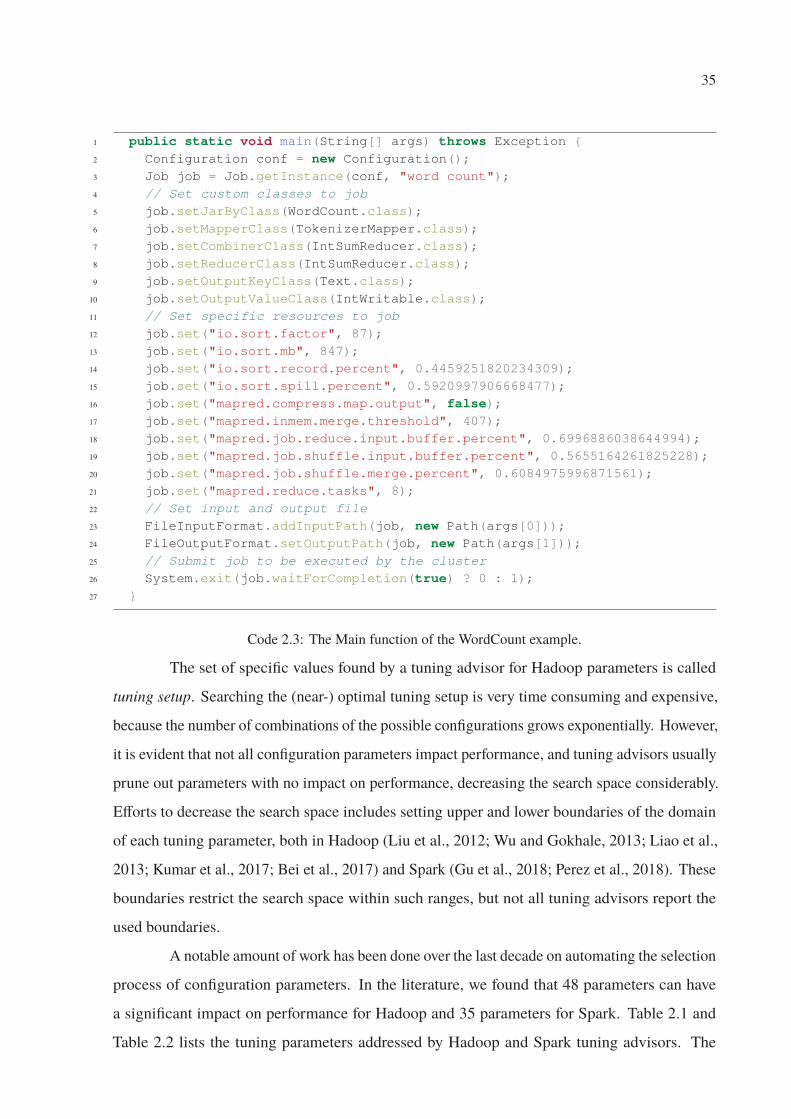
Administrators and developers can configure MapReduce jobs by hard-coding their configuration

in the source code, or instrumenting it via command line. Code 2.3 presents the main function of

the WordCount example, with hard-coded configuration. First, developers create an instance

of the MapReduce job, where this instance represents all the information required to guide the

MapReduce pipeline during the execution of this job. The required information includes the types

and custom classes used by each function of the MapReduce pipeline. Then, the configuration

parameters are set. In Code 2.3, 10 parameters are set. Note that the input and output paths are

also configured. In the end, the job is submitted to batch execution.

The execution behavior of MapReduce jobs is governed by several configuration

parameters that changes from version to version. Figure 2.3 presents the number of parameters

exposed by popular MapReduce and SQL-on-Hadoop engines through their releases. Note

that the number of parameters commonly increases along the evolution of the systems. This is

expected behavior due to the addition of new features. The number of configuration parameters

is important because they determine the number of possible configurations, i.e., the size of the

search space. For instance, while Pig and SparkSQL have about 100 parameters, Hive has almost

a thousand, which is an order of magnitude higher.

35

1 public static void main(String[] args) throws Exception {

2 Configuration conf = new Configuration();

3 Job job = Job.getInstance(conf, "word count");

4 // Set custom classes to job

5 job.setJarByClass(WordCount.class);

6 job.setMapperClass(TokenizerMapper.class);

7 job.setCombinerClass(IntSumReducer.class);

8 job.setReducerClass(IntSumReducer.class);

9 job.setOutputKeyClass(Text.class);

10 job.setOutputValueClass(IntWritable.class);

11 // Set specific resources to job

12 job.set("io.sort.factor", 87);

13 job.set("io.sort.mb", 847);

14 job.set("io.sort.record.percent", 0.4459251820234309);

15 job.set("io.sort.spill.percent", 0.5920997906668477);

16 job.set("mapred.compress.map.output", false);17 job.set("mapred.inmem.merge.threshold", 407);

18 job.set("mapred.job.reduce.input.buffer.percent", 0.6996886038644994);

19 job.set("mapred.job.shuffle.input.buffer.percent", 0.5655164261825228);

20 job.set("mapred.job.shuffle.merge.percent", 0.6084975996871561);

21 job.set("mapred.reduce.tasks", 8);

22 // Set input and output file

23 FileInputFormat.addInputPath(job, new Path(args[0]));

24 FileOutputFormat.setOutputPath(job, new Path(args[1]));

25 // Submit job to be executed by the cluster

26 System.exit(job.waitForCompletion(true) ? 0 : 1);

27 }

Code 2.3: The Main function of the WordCount example.

The set of specific values found by a tuning advisor for Hadoop parameters is called

tuning setup. Searching the (near-) optimal tuning setup is very time consuming and expensive,

because the number of combinations of the possible configurations grows exponentially. However,

it is evident that not all configuration parameters impact performance, and tuning advisors usually

prune out parameters with no impact on performance, decreasing the search space considerably.

Efforts to decrease the search space includes setting upper and lower boundaries of the domain

of each tuning parameter, both in Hadoop (Liu et al., 2012; Wu and Gokhale, 2013; Liao et al.,

2013; Kumar et al., 2017; Bei et al., 2017) and Spark (Gu et al., 2018; Perez et al., 2018). These

boundaries restrict the search space within such ranges, but not all tuning advisors report the

used boundaries.

A notable amount of work has been done over the last decade on automating the selection

process of configuration parameters. In the literature, we found that 48 parameters can have

a significant impact on performance for Hadoop and 35 parameters for Spark. Table 2.1 and

Table 2.2 lists the tuning parameters addressed by Hadoop and Spark tuning advisors. The

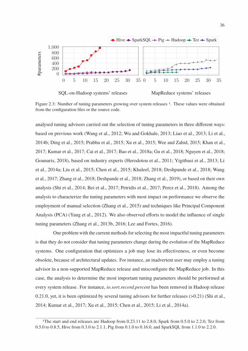
36

0 5 10 15 20 25 30 35

0200400600800

1,000

SQL-on-Hadoop systems’ releases

#par

amet

ers

0 5 10 15 20 25 30 35

MapReduce systems’ releases

Hive SparkSQL Pig Hadoop Tez Spark

Figure 2.3: Number of tuning parameters growing over system releases 1. These values were obtained

from the configuration files or the source code.

analysed tuning advisors carried out the selection of tuning parameters in three different ways:

based on previous work (Wang et al., 2012; Wu and Gokhale, 2013; Liao et al., 2013; Li et al.,

2014b; Ding et al., 2015; Prabhu et al., 2015; Xu et al., 2015; Wee and Zahid, 2015; Khan et al.,

2017; Kumar et al., 2017; Cai et al., 2017; Bao et al., 2018a; Gu et al., 2018; Nguyen et al., 2018;

Gounaris, 2018), based on industry experts (Herodotou et al., 2011; Yigitbasi et al., 2013; Li

et al., 2014a; Liu et al., 2015; Chen et al., 2015; Khaleel, 2018; Deshpande et al., 2018; Wang

et al., 2017; Zhang et al., 2018; Deshpande et al., 2018; Zhang et al., 2019), or based on their own

analysis (Shi et al., 2014; Bei et al., 2017; Petridis et al., 2017; Perez et al., 2018). Among the

analysis to characterize the tuning parameters with most impact on performance we observe the

employment of manual selection (Zhang et al., 2015) and techniques like Principal Component

Analysis (PCA) (Yang et al., 2012). We also observed efforts to model the influence of single

tuning parameters (Zhang et al., 2013b, 2016; Lee and Fortes, 2016).

One problem with the current methods for selecting the most impactful tuning parameters

is that they do not consider that tuning parameters change during the evolution of the MapReduce

systems. One configuration that optimizes a job may lose its effectiveness, or even become

obsolete, because of architectural updates. For instance, an inadvertent user may employ a tuning

advisor in a non-supported MapReduce release and misconfigure the MapReduce job. In this

case, the analysis to determine the most important tuning parameters should be performed at

every system release. For instance, io.sort.record.percent has been removed in Hadoop release

0.21.0, yet, it is been optimized by several tuning advisors for further releases (>0.21) (Shi et al.,

2014; Kumar et al., 2017; Xu et al., 2015; Chen et al., 2015; Li et al., 2014a).

1The start and end releases are Hadoop from 0.23.11 to 2.8.0, Spark from 0.5.0 to 2.2.0, Tez from

0.5.0 to 0.8.5, Hive from 0.3.0 to 2.1.1, Pig from 0.1.0 to 0.16.0, and SparkSQL from 1.1.0 to 2.2.0.

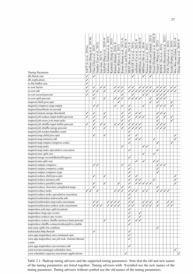
37

Tuning Parameter AA

CT

(Liet

al.,

2014a)

Auto

Tune

(Zhan

get

al.,

2013b)

Chen

(Chen

etal

.,2015)

Gunth

er(L

iao

etal

.,2013)

Jain

(Jai

n,2017)

�Je

llyFis

h(D

ing

etal

.,2015)

�

Johnst

on

(Johnst

on

etal

.,2015)

Kam

bat

la(Z

han

get

al.,

2015)

Khal

eel(K

hal

eel,

2018)

�K

han

(Khan

etal

.,2017)

Kum

ar(K

um

aret

al.,

2017)

�

Lee

(Lee

and

Fort

es,2016)

�

ME

ST

(Bei

etal

.,2017)

�M

R-C

OF

(Liu

etal

.,2015)

mrE

talo

n(C

aiet

al.,

2017)

�

MR

Online

(Liet

al.,

2014b)

�M

RTuner

(Shiet

al.,

2014)

Pan

acea

(Liu

etal

.,2012)

PPA

BS

(Wu

and

Gokhal

e,2013)

Pra

sad

(Des

hpan

de

etal

.,2018)

�Pre

dat

or

(Wan

get

al.,

2012)

RFH

OC

(Xu

etal

.,2015)

Sta

rfish

(Her

odoto

uet

al.,

2011)

SV

R(Y

igitbas

iet

al.,

2013)

Sw

athi(P

rabhu

etal

.,2015)

Wee

(Wee

and

Zah

id,2015)

�Z

han

g(Z

han

get

al.,

2016)

�

dfs.block.size � � � � �

dfs.replication �

io.file.buffer.size �

io.sort.factor � � � � � � � � � � � � � � � � � �

io.sort.mb � � � � � � � � � � � � � � � � � � � � �

io.sort.record.percent � � � � � � � � �

io.sort.spill.percent � � � � � � � � � � � � �

mapred.child.java.opts � � � �

mapred.compress.map.output � � � � � � � � � �

mapred.heartbeats.in.second �

mapred.inmem.merge.threshold � � � � � � � � � �

mapred.job.reduce.input.buffer.percent � � � � � � � � � � �

mapred.job.reuse.jvm.num.tasks � � � � �

mapred.job.shuffle.input.buffer.percent � � � � � � � � � � � � � �

mapred.job.shuffle.merge.percent � � � � � � � � � �

mapred.job.tracker.handler.count �

mapred.map.child.java.opts � � � � �

mapred.map.memory.mb � � � � �

mapred.map.output.compress.codec � � �

mapred.map.tasks � � �

mapred.map.tasks.speculative.execution � �

mapred.max.split.size � �

mapred.merge.recordsBeforeProgress �

mapred.min.split.size � � � �

mapred.output.compress � � � � � � �

mapred.output.compress.codec � �

mapred.output.compress.type � �

mapred.reduce.child.java.opts � � � � �

mapred.reduce.memory.mb � � � � �

mapred.reduce.parallel.copies � � � � � � � � � �

mapred.reduce.slowstart.completed.maps � � � �

mapred.reduce.tasks � � � � � � � � � � � � � � �

mapred.reduce.tasks.speculative.execution �

mapred.tasktracker.indexcache.mb �

mapred.tasktracker.map.tasks.maximum � � � � � � � � � � � � � �

mapred.tasktracker.reduce.tasks.maximum � � � � � � � � � � � � � � �

mapreduce.job.max.split.locations �

mapreduce.map.cpu.vcores � �

mapreduce.reduce.cpu.vcores � �

mapreduce.reduce.shuffle.memory.limit.percent � � � �

mapreduce.shuffle.connectionkeepalive.enable �

min.num.spills.for.combine �

tasktracker.http.threads � �

yarn.app.mapreduce.am.command-opts �

yarn.app.mapreduce.am.job.task.-listener.thread-

count

�

yarn.app.mapreduce.am.resource.mb �

yarn.resourcemanager.scheduler.class �

yarn.scheduler.capacity.maximum-applications � �

Table 2.1: Hadoop tuning advisers and the supported tuning parameters. Note that the old and new names

of the tuning parameters are listed together. Tuning advisers with �symbol use the new names of the

tuning parameter. Tuning advisers without symbol use the old names of the tuning parameters.

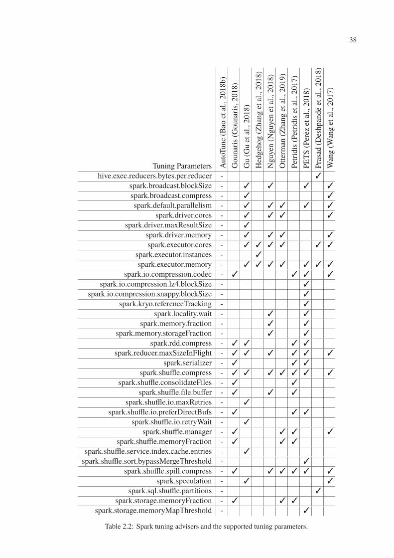
38

Tuning Parameters Auto

Tune

(Bao

etal

.,2018b)

Gounar

is(G

ounar

is,2018)

Gu

(Gu

etal

.,2018)

Hed

geh

og

(Zhan

get

al.,

2018)

Nguyen

(Nguyen

etal

.,2018)

Otter

man

(Zhan

get

al.,

2019)

Pet

ridis

(Pet

ridis

etal

.,2017)

PE

TS

(Per

ezet

al.,

2018)

Pra

sad

(Des

hpan

de

etal

.,2018)

Wan

g(W

ang

etal

.,2017)

hive.exec.reducers.bytes.per.reducer - �

spark.broadcast.blockSize - � � � �

spark.broadcast.compress - � �

spark.default.parallelism - � � � � �

spark.driver.cores - � � � �

spark.driver.maxResultSize - �

spark.driver.memory - � � � �

spark.executor.cores - � � � � � �

spark.executor.instances - �

spark.executor.memory - � � � � � � �

spark.io.compression.codec - � � � �

spark.io.compression.lz4.blockSize - �

spark.io.compression.snappy.blockSize - �

spark.kryo.referenceTracking - �

spark.locality.wait - � �

spark.memory.fraction - � �

spark.memory.storageFraction - � �

spark.rdd.compress - � � � �

spark.reducer.maxSizeInFlight - � � � � � �

spark.serializer - � � �

spark.shuffle.compress - � � � � � � �

spark.shuffle.consolidateFiles - � �

spark.shuffle.file.buffer - � � �

spark.shuffle.io.maxRetries - �

spark.shuffle.io.preferDirectBufs - � � �

spark.shuffle.io.retryWait - �

spark.shuffle.manager - � � � �

spark.shuffle.memoryFraction - � � �

spark.shuffle.service.index.cache.entries - �

spark.shuffle.sort.bypassMergeThreshold - �

spark.shuffle.spill.compress - � � � � � �

spark.speculation - � �

spark.sql.shuffle.partitions - �

spark.storage.memoryFraction - � � �

spark.storage.memoryMapThreshold - �

Table 2.2: Spark tuning advisers and the supported tuning parameters.

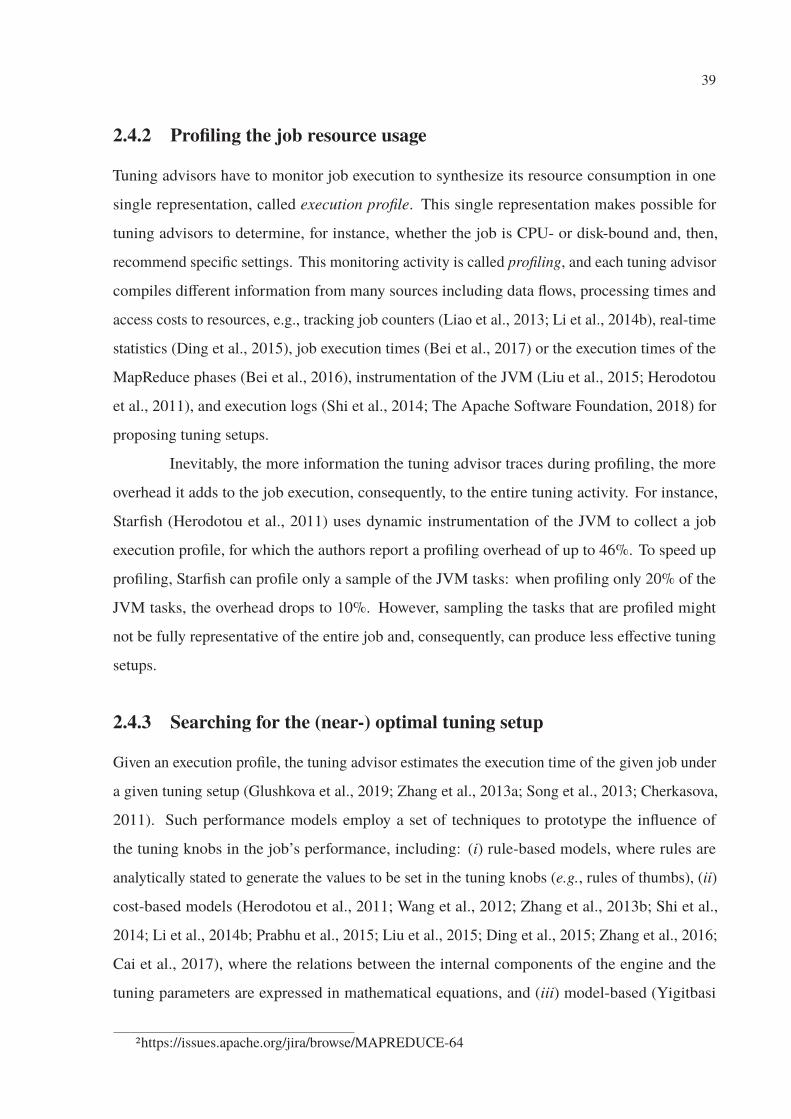
39

2.4.2 Profiling the job resource usage

Tuning advisors have to monitor job execution to synthesize its resource consumption in one

single representation, called execution profile. This single representation makes possible for

tuning advisors to determine, for instance, whether the job is CPU- or disk-bound and, then,

recommend specific settings. This monitoring activity is called profiling, and each tuning advisor

compiles different information from many sources including data flows, processing times and

access costs to resources, e.g., tracking job counters (Liao et al., 2013; Li et al., 2014b), real-time

statistics (Ding et al., 2015), job execution times (Bei et al., 2017) or the execution times of the

MapReduce phases (Bei et al., 2016), instrumentation of the JVM (Liu et al., 2015; Herodotou

et al., 2011), and execution logs (Shi et al., 2014; The Apache Software Foundation, 2018) for

proposing tuning setups.

Inevitably, the more information the tuning advisor traces during profiling, the more

overhead it adds to the job execution, consequently, to the entire tuning activity. For instance,

Starfish (Herodotou et al., 2011) uses dynamic instrumentation of the JVM to collect a job

execution profile, for which the authors report a profiling overhead of up to 46%. To speed up

profiling, Starfish can profile only a sample of the JVM tasks: when profiling only 20% of the

JVM tasks, the overhead drops to 10%. However, sampling the tasks that are profiled might

not be fully representative of the entire job and, consequently, can produce less effective tuning

setups.

2.4.3 Searching for the (near-) optimal tuning setup

Given an execution profile, the tuning advisor estimates the execution time of the given job under

a given tuning setup (Glushkova et al., 2019; Zhang et al., 2013a; Song et al., 2013; Cherkasova,

2011). Such performance models employ a set of techniques to prototype the influence of

the tuning knobs in the job’s performance, including: (i) rule-based models, where rules are

analytically stated to generate the values to be set in the tuning knobs (e.g., rules of thumbs), (ii)

cost-based models (Herodotou et al., 2011; Wang et al., 2012; Zhang et al., 2013b; Shi et al.,

2014; Li et al., 2014b; Prabhu et al., 2015; Liu et al., 2015; Ding et al., 2015; Zhang et al., 2016;

Cai et al., 2017), where the relations between the internal components of the engine and the

tuning parameters are expressed in mathematical equations, and (iii) model-based (Yigitbasi

2https://issues.apache.org/jira/browse/MAPREDUCE-64

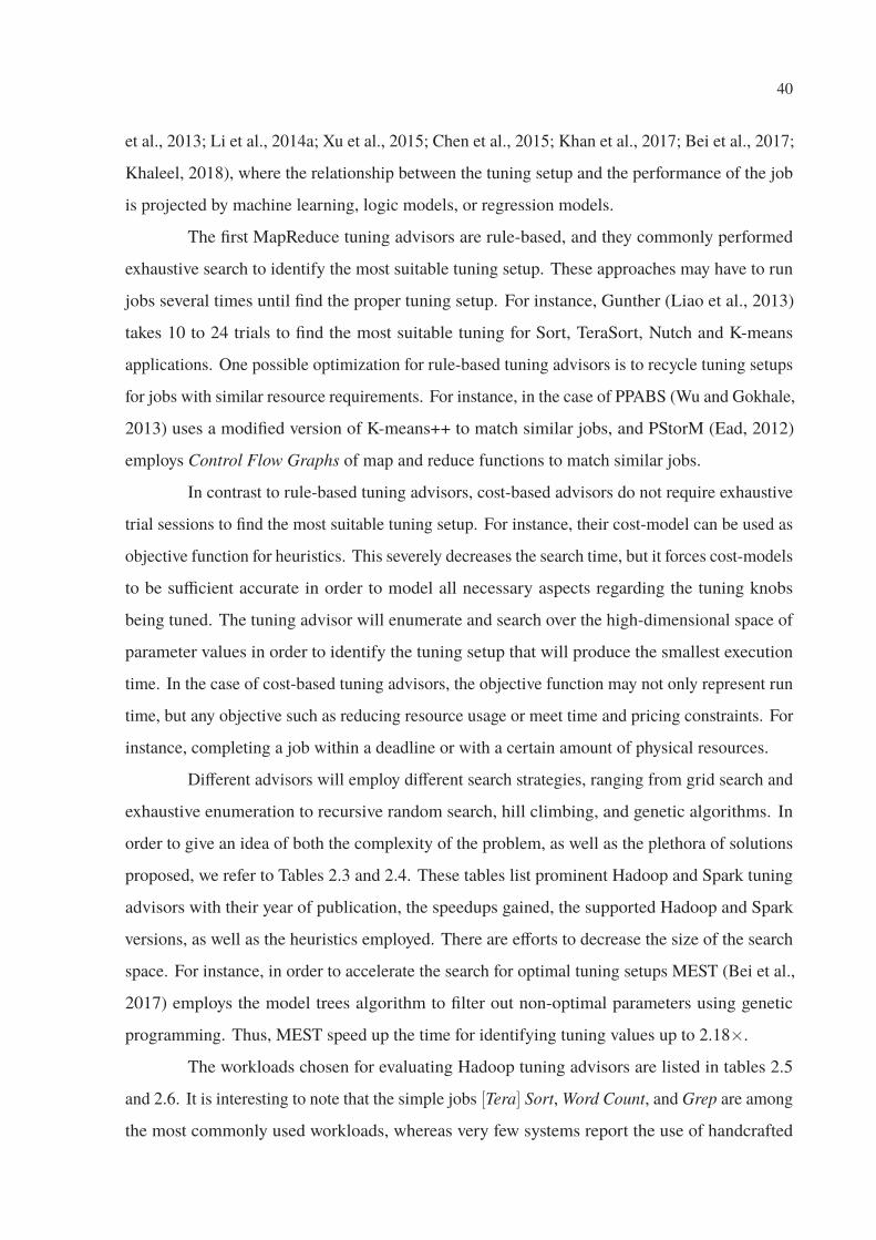
40

et al., 2013; Li et al., 2014a; Xu et al., 2015; Chen et al., 2015; Khan et al., 2017; Bei et al., 2017;

Khaleel, 2018), where the relationship between the tuning setup and the performance of the job

is projected by machine learning, logic models, or regression models.

The first MapReduce tuning advisors are rule-based, and they commonly performed

exhaustive search to identify the most suitable tuning setup. These approaches may have to run

jobs several times until find the proper tuning setup. For instance, Gunther (Liao et al., 2013)

takes 10 to 24 trials to find the most suitable tuning for Sort, TeraSort, Nutch and K-means

applications. One possible optimization for rule-based tuning advisors is to recycle tuning setups

for jobs with similar resource requirements. For instance, in the case of PPABS (Wu and Gokhale,

2013) uses a modified version of K-means++ to match similar jobs, and PStorM (Ead, 2012)

employs Control Flow Graphs of map and reduce functions to match similar jobs.

In contrast to rule-based tuning advisors, cost-based advisors do not require exhaustive

trial sessions to find the most suitable tuning setup. For instance, their cost-model can be used as

objective function for heuristics. This severely decreases the search time, but it forces cost-models

to be sufficient accurate in order to model all necessary aspects regarding the tuning knobs

being tuned. The tuning advisor will enumerate and search over the high-dimensional space of

parameter values in order to identify the tuning setup that will produce the smallest execution

time. In the case of cost-based tuning advisors, the objective function may not only represent run

time, but any objective such as reducing resource usage or meet time and pricing constraints. For

instance, completing a job within a deadline or with a certain amount of physical resources.

Different advisors will employ different search strategies, ranging from grid search and

exhaustive enumeration to recursive random search, hill climbing, and genetic algorithms. In

order to give an idea of both the complexity of the problem, as well as the plethora of solutions

proposed, we refer to Tables 2.3 and 2.4. These tables list prominent Hadoop and Spark tuning

advisors with their year of publication, the speedups gained, the supported Hadoop and Spark

versions, as well as the heuristics employed. There are efforts to decrease the size of the search

space. For instance, in order to accelerate the search for optimal tuning setups MEST (Bei et al.,

2017) employs the model trees algorithm to filter out non-optimal parameters using genetic

programming. Thus, MEST speed up the time for identifying tuning values up to 2.18×.

The workloads chosen for evaluating Hadoop tuning advisors are listed in tables 2.5

and 2.6. It is interesting to note that the simple jobs [Tera] Sort, Word Count, and Grep are among

the most commonly used workloads, whereas very few systems report the use of handcrafted

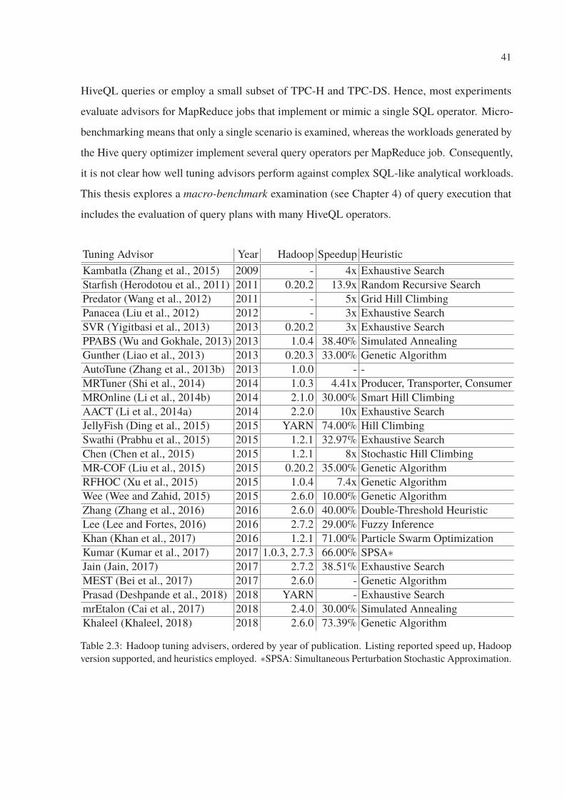
41

HiveQL queries or employ a small subset of TPC-H and TPC-DS. Hence, most experiments

evaluate advisors for MapReduce jobs that implement or mimic a single SQL operator. Micro-

benchmarking means that only a single scenario is examined, whereas the workloads generated by

the Hive query optimizer implement several query operators per MapReduce job. Consequently,

it is not clear how well tuning advisors perform against complex SQL-like analytical workloads.

This thesis explores a macro-benchmark examination (see Chapter 4) of query execution that

includes the evaluation of query plans with many HiveQL operators.

Tuning Advisor Year Hadoop Speedup Heuristic

Kambatla (Zhang et al., 2015) 2009 - 4x Exhaustive Search

Starfish (Herodotou et al., 2011) 2011 0.20.2 13.9x Random Recursive Search

Predator (Wang et al., 2012) 2011 - 5x Grid Hill Climbing

Panacea (Liu et al., 2012) 2012 - 3x Exhaustive Search

SVR (Yigitbasi et al., 2013) 2013 0.20.2 3x Exhaustive Search

PPABS (Wu and Gokhale, 2013) 2013 1.0.4 38.40% Simulated Annealing

Gunther (Liao et al., 2013) 2013 0.20.3 33.00% Genetic Algorithm

AutoTune (Zhang et al., 2013b) 2013 1.0.0 - -

MRTuner (Shi et al., 2014) 2014 1.0.3 4.41x Producer, Transporter, Consumer

MROnline (Li et al., 2014b) 2014 2.1.0 30.00% Smart Hill Climbing

AACT (Li et al., 2014a) 2014 2.2.0 10x Exhaustive Search

JellyFish (Ding et al., 2015) 2015 YARN 74.00% Hill Climbing

Swathi (Prabhu et al., 2015) 2015 1.2.1 32.97% Exhaustive Search

Chen (Chen et al., 2015) 2015 1.2.1 8x Stochastic Hill Climbing

MR-COF (Liu et al., 2015) 2015 0.20.2 35.00% Genetic Algorithm

RFHOC (Xu et al., 2015) 2015 1.0.4 7.4x Genetic Algorithm

Wee (Wee and Zahid, 2015) 2015 2.6.0 10.00% Genetic Algorithm

Zhang (Zhang et al., 2016) 2016 2.6.0 40.00% Double-Threshold Heuristic

Lee (Lee and Fortes, 2016) 2016 2.7.2 29.00% Fuzzy Inference

Khan (Khan et al., 2017) 2016 1.2.1 71.00% Particle Swarm Optimization

Kumar (Kumar et al., 2017) 2017 1.0.3, 2.7.3 66.00% SPSA∗Jain (Jain, 2017) 2017 2.7.2 38.51% Exhaustive Search

MEST (Bei et al., 2017) 2017 2.6.0 - Genetic Algorithm

Prasad (Deshpande et al., 2018) 2018 YARN - Exhaustive Search

mrEtalon (Cai et al., 2017) 2018 2.4.0 30.00% Simulated Annealing

Khaleel (Khaleel, 2018) 2018 2.6.0 73.39% Genetic Algorithm

Table 2.3: Hadoop tuning advisers, ordered by year of publication. Listing reported speed up, Hadoop

version supported, and heuristics employed. ∗SPSA: Simultaneous Perturbation Stochastic Approximation.

42

Tuning Adviser Year Spark Speedup Heuristic

Petridis (Petridis et al., 2017) 2017 1.5.2 10x Trial-and-Error

Wang (Wang et al., 2017) 2017 1.6.1 36% Recursive Random Search

AutoTune (Bao et al., 2018a) 2018 - 63.7% Two-Step Multiple Bound

Gounaris (Gounaris, 2018) 2018 1.5.2 4x Greedy Algorithm

Gu (Gu et al., 2018) 2018 - 42.8% Neural Network

Hedgehog (Zhang et al., 2018) 2018 2.1 19.6% Marginal Utility Law

Nguyen (Nguyen et al., 2018) 2018 2.0.2 40.0% Recursive Random Search

PETS (Perez et al., 2018) 2018 4.78x 82% Fuzzy Inference

Prasad (Deshpande et al., 2018) 2018 - - Exhaustive Search

Otterman (Zhang et al., 2019) 2019 2.2.0 30% Simulated Annealing

Table 2.4: Spark tuning advisers, ordered by year of publication. Listing reported speed up, supported

version, and the heuristic employed.

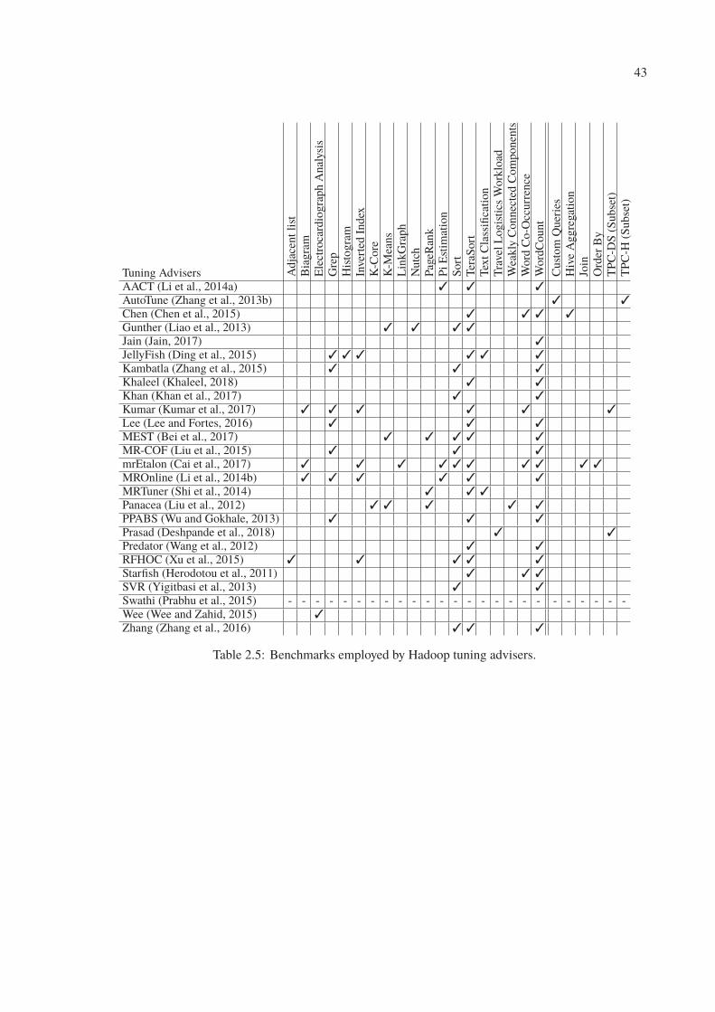
43

Tuning Advisers Adja

centlist

Bia

gra

m

Ele

ctro

card

iogra

ph

Anal

ysi

s

Gre

p

His

togra

m

Inver

ted

Index

K-C

ore

K-M

eans

Lin

kG

raph

Nutc

h

Pag

eRan

k

PiE

stim

atio

n

Sort

Ter

aSort

Tex

tC

lass

ifica

tion

Tra

vel

Logis

tics

Work

load

Wea

kly

Connec

ted

Com

ponen

ts

Word

Co-O

ccurr

ence

Word

Count

Cust

om

Quer

ies

Hiv

eA

ggre

gat

ion

Join

Ord

erB

y

TPC

-DS

(Subse

t)

TPC

-H(S

ubse

t)

AACT (Li et al., 2014a) � � �AutoTune (Zhang et al., 2013b) � �Chen (Chen et al., 2015) � � � �Gunther (Liao et al., 2013) � � � �Jain (Jain, 2017) �JellyFish (Ding et al., 2015) � � � � � �Kambatla (Zhang et al., 2015) � � �Khaleel (Khaleel, 2018) � �Khan (Khan et al., 2017) � �Kumar (Kumar et al., 2017) � � � � � �Lee (Lee and Fortes, 2016) � � �MEST (Bei et al., 2017) � � � � �MR-COF (Liu et al., 2015) � � �mrEtalon (Cai et al., 2017) � � � � � � � � � �MROnline (Li et al., 2014b) � � � � � �MRTuner (Shi et al., 2014) � � �Panacea (Liu et al., 2012) � � � � �PPABS (Wu and Gokhale, 2013) � � �Prasad (Deshpande et al., 2018) � �Predator (Wang et al., 2012) � �RFHOC (Xu et al., 2015) � � � � �Starfish (Herodotou et al., 2011) � � �SVR (Yigitbasi et al., 2013) � �Swathi (Prabhu et al., 2015) - - - - - - - - - - - - - - - - - - - - - - - - -

Wee (Wee and Zahid, 2015) �Zhang (Zhang et al., 2016) � � �

Table 2.5: Benchmarks employed by Hadoop tuning advisers.

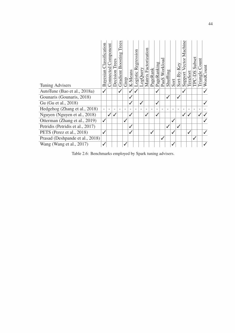
44

Tuning Advisers Bay

esia

nC

lass

ifica

tion

Connec

ted

Com

ponen

t

Dec

isio

nT

rees

Gra

die

ntB

oost

ing

Tre

es

Gre

p

K-M

eans

Logis

tic

Reg

ress

ion

LogQ

uer

y

Mat

rix

Fac

tori

zation

Pag

eRan

k

Pag

eRan

kin

g

Paa

SW

ork

load

Shuffl

ing

Sort

Sort

-By-K

ey

Support

Vec

tor

Mac

hin

e

Ter

aSort

TPC

-DS

Subse

t

Tri

angle

Count

Word

Count

AutoTune (Bao et al., 2018a) � � � � � � �

Gounaris (Gounaris, 2018) � � �

Gu (Gu et al., 2018) � � � �

Hedgehog (Zhang et al., 2018) - - - - - - - - - - - - - - - - - - - -

Nguyen (Nguyen et al., 2018) � � � � � � � � �

Otterman (Zhang et al., 2019) � � � �

Petridis (Petridis et al., 2017) � � �

PETS (Perez et al., 2018) � � � � � �

Prasad (Deshpande et al., 2018) � �

Wang (Wang et al., 2017) � � � �

Table 2.6: Benchmarks employed by Spark tuning advisers.

45

2.5 Query Execution in Hive

Hive (Thusoo et al., 2010), an open source project originally built at Facebook, was the first

SQL-on-Hadoop query engine built on top of Hadoop MapReduce to leverage its scalability, fault

tolerance, and scheduling features. Hive also introduced HiveQL, a SQL-like query language

that has become the standard SQL interface for large-scale data (Floratou et al., 2014). Hive

can process structured and semi-structured data. Code 2.4 presents a Hive example of a query

for loading semi-structured data from logs of the Apache Web Server. Hive also can read a

number of semi-structured formats such as JSON and XML, and many other formats including

Avro, ORC, Parquet and CSV. Hive also enables developers to write their own Serialization and

De-serialization libraries.

Hive internally uses a query optimizer that resembles traditional relational optimizers to

translate a given HiveQL statement to a workflow of MapReduce jobs to be executed on Hadoop.

Specifically, a HiveQL statement is first parsed and validated against the data dictionary, compiled

into a tree of logical operators, and finally optimized to produce a physical query execution plan

(Floratou et al., 2014; Thusoo et al., 2010). This allows for various logical optimizations such as

selection and projection pushdowns, as well as join reordering and join physical method selection.

Physical-layer tuning such as partition pruning is also performed when an input table is split

over several HDFS folders to avoid processing unnecessary data (Huai et al., 2014). The final

execution plan has the form of a Directed Acyclic Graph (DAG) of MapReduce jobs. Each job is

executed on the cluster as a set of parallel Map and Reduce tasks. By now, Hive supports other

execution engines such as Spark and Tez.

As a further, MapReduce-specific optimization, the Hive query optimizer merges jobs

by applying chain folding and job merging, which are both considered generic MapReduce design

patterns (Miner and Shook, 2012b). As a simple example, chain folding collapses sequences

of Map-only jobs into a single Map-only job (In Hive and Spark terminology, merged jobs are

called stages. This thesis follows the convention of Hadoop processing and use the general

term job). Job merging further merges jobs that process the same input data, such as joins

applying a common join predicate. Hence, each resulting MapReduce job will typically evaluate

several query operators. Similar optimizations have also been proposed in Stubby (Lim et al.,

2012), YSmart (Lee et al., 2011), and MRShare (Nykiel et al., 2010) as they are very effective in

speeding up query execution by reducing the number of intermediate files that are written out to

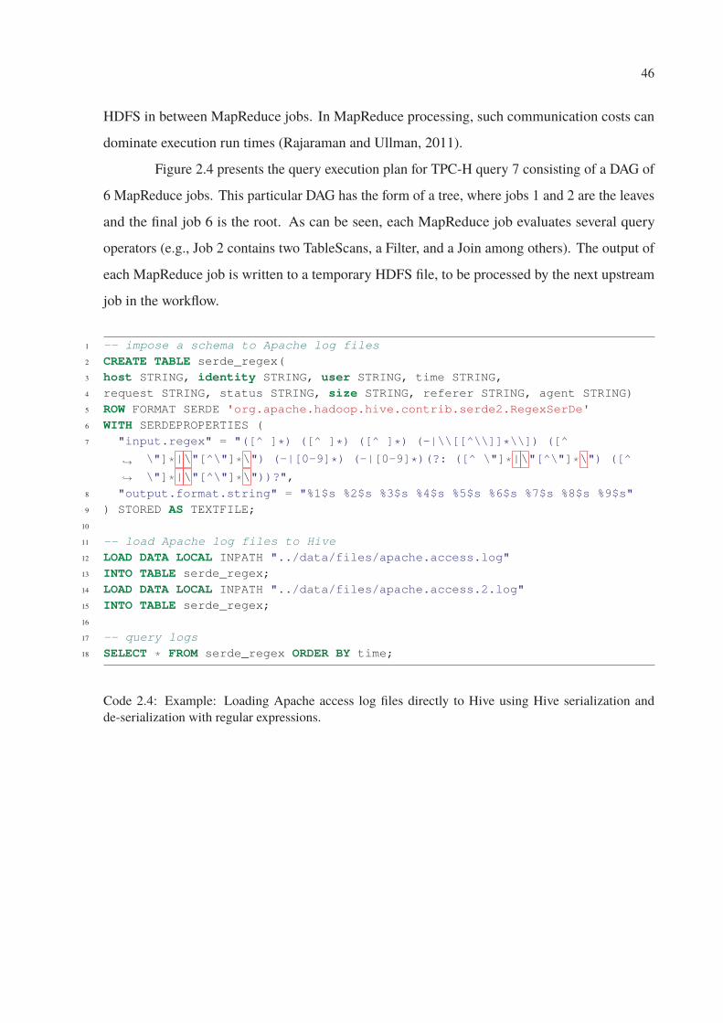
46

HDFS in between MapReduce jobs. In MapReduce processing, such communication costs can

dominate execution run times (Rajaraman and Ullman, 2011).

Figure 2.4 presents the query execution plan for TPC-H query 7 consisting of a DAG of

6 MapReduce jobs. This particular DAG has the form of a tree, where jobs 1 and 2 are the leaves

and the final job 6 is the root. As can be seen, each MapReduce job evaluates several query

operators (e.g., Job 2 contains two TableScans, a Filter, and a Join among others). The output of

each MapReduce job is written to a temporary HDFS file, to be processed by the next upstream

job in the workflow.

1 -- impose a schema to Apache log files

2 CREATE TABLE serde_regex(

3 host STRING, identity STRING, user STRING, time STRING,

4 request STRING, status STRING, size STRING, referer STRING, agent STRING)

5 ROW FORMAT SERDE 'org.apache.hadoop.hive.contrib.serde2.RegexSerDe'

6 WITH SERDEPROPERTIES (

7 "input.regex" = "([^ ]*) ([^ ]*) ([^ ]*) (-|\\[[^\\]]*\\]) ([^

\"]*|\"[^\"]*\") (-|[0-9]*) (-|[0-9]*)(?: ([^ \"]*|\"[^\"]*\") ([^

\"]*|\"[^\"]*\"))?",

↪→

↪→

8 "output.format.string" = "%1$s %2$s %3$s %4$s %5$s %6$s %7$s %8$s %9$s"

9 ) STORED AS TEXTFILE;

10

11 -- load Apache log files to Hive

12 LOAD DATA LOCAL INPATH "../data/files/apache.access.log"

13 INTO TABLE serde_regex;

14 LOAD DATA LOCAL INPATH "../data/files/apache.access.2.log"

15 INTO TABLE serde_regex;

16

17 -- query logs

18 SELECT * FROM serde_regex ORDER BY time;

Code 2.4: Example: Loading Apache access log files directly to Hive using Hive serialization and

de-serialization with regular expressions.

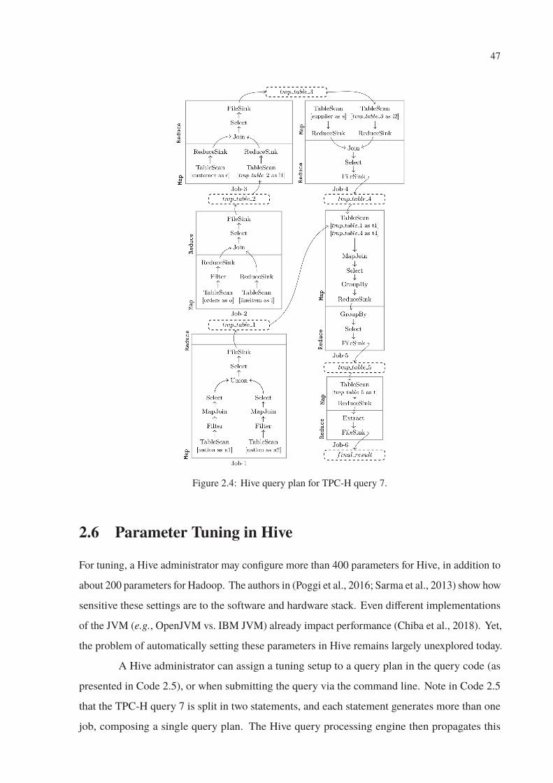
47

Figure 2.4: Hive query plan for TPC-H query 7.

2.6 Parameter Tuning in Hive

For tuning, a Hive administrator may configure more than 400 parameters for Hive, in addition to

about 200 parameters for Hadoop. The authors in (Poggi et al., 2016; Sarma et al., 2013) show how

sensitive these settings are to the software and hardware stack. Even different implementations

of the JVM (e.g., OpenJVM vs. IBM JVM) already impact performance (Chiba et al., 2018). Yet,

the problem of automatically setting these parameters in Hive remains largely unexplored today.

A Hive administrator can assign a tuning setup to a query plan in the query code (as

presented in Code 2.5), or when submitting the query via the command line. Note in Code 2.5

that the TPC-H query 7 is split in two statements, and each statement generates more than one

job, composing a single query plan. The Hive query processing engine then propagates this

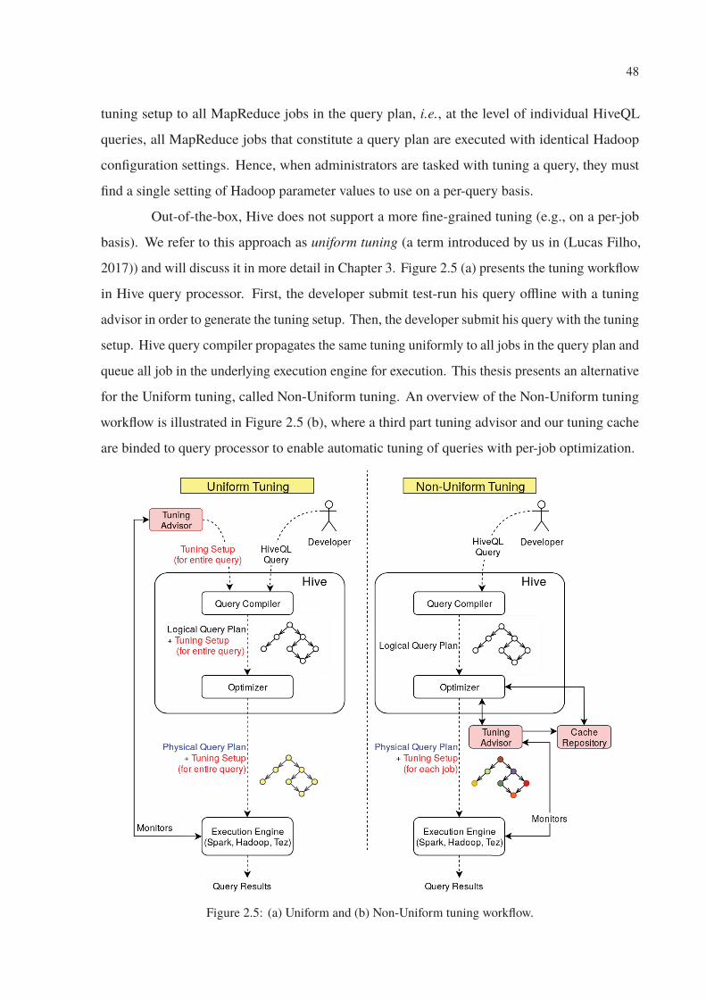
48

tuning setup to all MapReduce jobs in the query plan, i.e., at the level of individual HiveQL

queries, all MapReduce jobs that constitute a query plan are executed with identical Hadoop

configuration settings. Hence, when administrators are tasked with tuning a query, they must

find a single setting of Hadoop parameter values to use on a per-query basis.

Out-of-the-box, Hive does not support a more fine-grained tuning (e.g., on a per-job

basis). We refer to this approach as uniform tuning (a term introduced by us in (Lucas Filho,

2017)) and will discuss it in more detail in Chapter 3. Figure 2.5 (a) presents the tuning workflow

in Hive query processor. First, the developer submit test-run his query offline with a tuning

advisor in order to generate the tuning setup. Then, the developer submit his query with the tuning

setup. Hive query compiler propagates the same tuning uniformly to all jobs in the query plan and

queue all job in the underlying execution engine for execution. This thesis presents an alternative

for the Uniform tuning, called Non-Uniform tuning. An overview of the Non-Uniform tuning

workflow is illustrated in Figure 2.5 (b), where a third part tuning advisor and our tuning cache

are binded to query processor to enable automatic tuning of queries with per-job optimization.

Figure 2.5: (a) Uniform and (b) Non-Uniform tuning workflow.

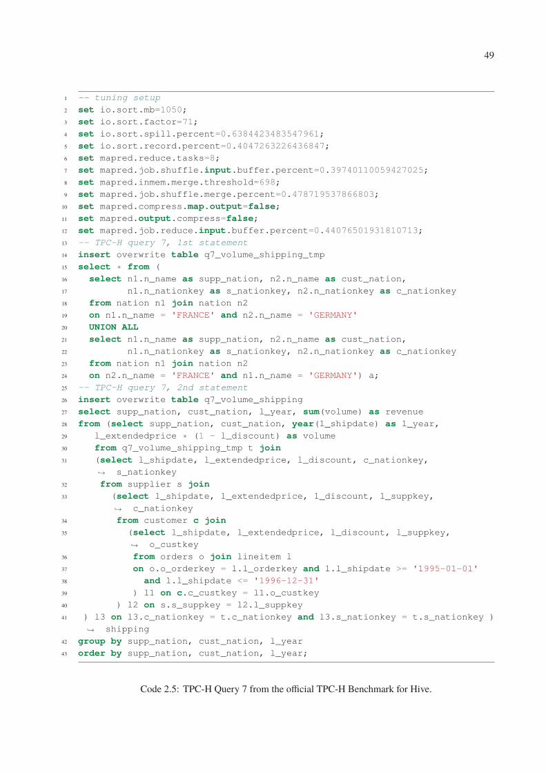
49

1 -- tuning setup

2 set io.sort.mb=1050;

3 set io.sort.factor=71;

4 set io.sort.spill.percent=0.6384423483547961;

5 set io.sort.record.percent=0.4047263226436847;

6 set mapred.reduce.tasks=8;

7 set mapred.job.shuffle.input.buffer.percent=0.39740110059427025;8 set mapred.inmem.merge.threshold=698;

9 set mapred.job.shuffle.merge.percent=0.478719537866803;

10 set mapred.compress.map.output=false;11 set mapred.output.compress=false;12 set mapred.job.reduce.input.buffer.percent=0.44076501931810713;13 -- TPC-H query 7, 1st statement

14 insert overwrite table q7_volume_shipping_tmp

15 select * from (

16 select n1.n_name as supp_nation, n2.n_name as cust_nation,

17 n1.n_nationkey as s_nationkey, n2.n_nationkey as c_nationkey

18 from nation n1 join nation n2

19 on n1.n_name = 'FRANCE' and n2.n_name = 'GERMANY'

20 UNION ALL21 select n1.n_name as supp_nation, n2.n_name as cust_nation,

22 n1.n_nationkey as s_nationkey, n2.n_nationkey as c_nationkey

23 from nation n1 join nation n2

24 on n2.n_name = 'FRANCE' and n1.n_name = 'GERMANY') a;

25 -- TPC-H query 7, 2nd statement

26 insert overwrite table q7_volume_shipping

27 select supp_nation, cust_nation, l_year, sum(volume) as revenue

28 from (select supp_nation, cust_nation, year(l_shipdate) as l_year,

29 l_extendedprice * (1 - l_discount) as volume

30 from q7_volume_shipping_tmp t join31 (select l_shipdate, l_extendedprice, l_discount, c_nationkey,

s_nationkey↪→

32 from supplier s join33 (select l_shipdate, l_extendedprice, l_discount, l_suppkey,

c_nationkey↪→

34 from customer c join35 (select l_shipdate, l_extendedprice, l_discount, l_suppkey,

o_custkey↪→

36 from orders o join lineitem l

37 on o.o_orderkey = l.l_orderkey and l.l_shipdate >= '1995-01-01'

38 and l.l_shipdate <= '1996-12-31'

39 ) l1 on c.c_custkey = l1.o_custkey

40 ) l2 on s.s_suppkey = l2.l_suppkey

41 ) l3 on l3.c_nationkey = t.c_nationkey and l3.s_nationkey = t.s_nationkey )

shipping↪→

42 group by supp_nation, cust_nation, l_year

43 order by supp_nation, cust_nation, l_year;

Code 2.5: TPC-H Query 7 from the official TPC-H Benchmark for Hive.

50

Chapter 3

Tuning SQL-on-Hadoop Systems

In this Chapter we formulate the problem of finding the most efficient tuning setup for SQL-on-

Hadoop query plans. We present an experimental analysis of the impact of the uniform parameter

tuning on the execution of HiveQL queries to motivate our contributions in the upcoming chapters.

We also explore the costs of the Uniform Tuning approach, used by current SQL-on-Hadoop

systems.

3.1 The SQL-on-Hadoop Tuning Problem

First, let us formulate the search for the optimal tuning setup for a single MapReduce job. Let us

define a MapReduce job j as a tuple of the form j = (O,D,C), in which O is the set of code it

executes (e.g., MapReduce functions implementing several relational algebra operators), D is the

set of data that are read and processed by j, and C is the set of configuration parameters exposed

by the processing engine (e.g., Hadoop, Spark, Tez) that is used to allocate resources to job j,

where every configuration parameter ci ∈ C has a different domain dom(ci) of size si.

Now, suppose that we have a computable function σ : J × C �→ R, where J is a set of

possible MapReduce jobs, and C = {C1, . . . , Ck} is the collection of all possible configurations,

and the function σ(j, Ci) determines the computational cost of executing job j under the tuning

setup Ci. We define the task of searching for the most efficient tuning setup for a single

MapReduce job (where the most efficient tuning setup is the configuration that minimizes the

response time or the resource usage of a MapReduce job) as the Advisor Function, as follows:

51

Definition 1 (Advisor Function): Given a set C representing all possible configuration param-

eters, and a cost function σ : J × C �→ R. We denote as f(j) the advisor function f : J �→ Cwhich is responsible for finding the most efficient tuning setup Cj for a given j ∈ J such that:

f(j) = Cj = minCx∈C

σ(j, Cx) (3.1)

The Advisor Function is implemented by third part Tuning Advisors that employ a

diverse set of modeling and searching techniques for finding optimal tuning setups, as detailed in

Chapter 2. Equation 3.1 models the search for the tuning setup for a given job, which always

finds the optimal tuning setup for a given job. However, in practice, Tuning Advisors employ

approximation techniques such as search heuristics due to the high dimensionality of the problem.

Consequently, Tuning Advisors always generate sub optimal results.

Thus, Tuning Advisors generate sub-optimal results because of: (i) modeling techniques

that may fail to model important aspects of the system that have dynamic characteristics, such

as updates in the hardware stack or natural evolution of the data sets, and (ii) the employment

of search heuristics that have no guarantee of optimality for high dimensional spaces, such as

Genetic Algorithm (Liao et al., 2013; Liu et al., 2015; Bei et al., 2017), and Particle Swarm

Optimization (Khan et al., 2017).

Now, let us formulate the search for the optimal tuning setup for a SQL-on-Hadoop

query. We use the TPC-H query 7 as a running example. Figure 2.4 illustrates in details the

query plan for query 7 executing in Hive version 0.13.1, presenting the operators executed in the

Map and Reduce phases as well as the tables that read. The complexity of the query plans grows

across releases as the SQL-on-Hadoop query processing engines add support to new optimization

techniques, operators, data format, etc. For instance, Figure 3.1 illustrates the compiled for two

different versions of Hive, specifically, version 0.13.1 and 3.1.0. Observe that the query plan of

query in Hive 3.1.0 has 3× more jobs than the query plan generated by Hive 0.13.1.

Let us define a SQL-on-Hadoop’s query plan as a directed acyclic graph G = (V,E),

where the set of vertices V represents MapReduce jobs, and the set of edges E denotes the

precedence between two jobs. Each directed edge is an ordered pair of vertices e = (vi, vj) ∈ E

that connects the jobs vi to vj , when the execution of vi directly precedes vj , depicted in Figure 3.1.

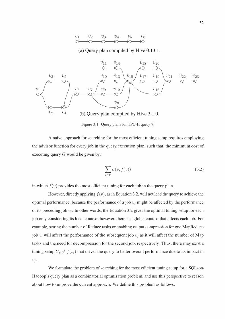
52

v1 v2 v3 v4 v5 v6

v1

v2

v3

v4

v5

v6 v7

v8

v9

v10

v11

v12

v13

v14

v15

v16

v17

v18

v19

v20

v21 v22 v23

(a) Query plan compiled by Hive 0.13.1.

(b) Query plan compiled by Hive 3.1.0.

Figure 3.1: Query plans for TPC-H query 7.

A naive approach for searching for the most efficient tuning setup requires employing

the advisor function for every job in the query execution plan, such that, the minimum cost of

executing query G would be given by:

∑v∈V

σ(v, f(v)) (3.2)

in which f(v) provides the most efficient tuning for each job in the query plan.

However, directly applying f(v), as in Equation 3.2, will not lead the query to achieve the

optimal performance, because the performance of a job vj might be affected by the performance

of its preceding job vi. In other words, the Equation 3.2 gives the optimal tuning setup for each

job only considering its local context, however, there is a global context that affects each job. For

example, setting the number of Reduce tasks or enabling output compression for one MapReduce

job vi will affect the performance of the subsequent job vj as it will affect the number of Map

tasks and the need for decompression for the second job, respectively. Thus, there may exist a

tuning setup Cx �= f(vi) that drives the query to better overall performance due to its impact in

vj .

We formulate the problem of searching for the most efficient tuning setup for a SQL-on-

Hadoop’s query plan as a combinatorial optimization problem, and use this perspective to reason

about how to improve the current approach. We define this problem as follows:

53

Definition 2 (SQL-on-Hadoop’s Tuning Problem): Given a directed acyclic graph G =

(V,E) representing a SQL-on-Hadoop’s query plan, a set C of all possible configurations,

and a cost function σ : V × C → R. Find the subset of configuration parameters C ′ ⊂ C , that

contains every element Cv ∈ C ′ associated to an element v ∈ V , such that, the total cost to

process the G is minimum, that is, considering the global context of each job, minimize

∑Cv∈C′

σ(v, Cv) (3.3)

Equation 3.3 finds the optimal tuning setup for a given query plan G, while Equation 3.2

finds sub-optimal setups. However, Equation 3.3 has to evaluate the tuning setup of each job

considering the tuning setup of its preceding jobs, in a “back-tracking” fashion. On the opposite,

Equation 3.2 has to evaluate the configuration of each job, without considering its preceding

jobs. Thus, because of the large size of the search space the number of evaluations performed by

Equation 3.3 might be higher than Equation 3.2, which directly impacts on the time for searching

for the optimal tuning setup.

3.2 The Uniform Tuning Approach

The current tuning strategy used by SQL-on-Hadoop processing engines allocates the same

physical resources to all jobs of a query plan by propagating the same tuning setup through the

query plan. We name this approach as Uniform Tuning, and define it as follows:

Definition 3 (Uniform Tuning): The Uniform Tuning strategy is the assignment of configura-

tions to jobs such that Cu = Cv for u, v ∈ V and Cu, Cv ∈ C.

Despite the adviser function f(v) finds the most efficient tuning setup Cv for every job

v ∈ V , in the case of the Uniform Tuning only one tuning setup Cv is chosen to be propagated to

all jobs in V . Thus, in Uniform Tuning Cv improve the performance of some jobs at the expense

of negatively affecting the performance of other jobs, impacting the overall performance. We

execute the 22 TPC-H benchmark queries with all possible tuning setups in order to analyze the

impact of the Uniform Tuning. The results of the impact of the Uniform Tuning presented in the

following sections motivate our contributions.

54

3.2.1 Experiment Setup

Before analyzing the impact of the uniform Tuning, we present the environment used in all the

experiments of this chapter. Our execution environment is a cluster of 10 machines (m5.2xlarge1

with 8 CPU cores, 32 GiB of RAM, 500 GiB of disk), hosted at Amazon Web Services (AWS)

cloud environment. The cluster runs Ubuntu 16.04 with Hive 0.13.1, Hadoop 0.22.2, and

Starfish 0.32. These specific Hadoop and Hive versions are those supported by the latest version

of Starfish. The HDFS replication factor is set to 3 and the default block size is 128MB. The

maximum number of Map and Reduce tasks that can be started on each node is set to fit the

maximum capacity of the CPU (8 threads per node).

For our evaluation, we use TPC-H (TPC), a standard decision support benchmark

consisting of 22 queries over 8 tables. Even though TPC-H was developed for evaluating

traditional relational database systems, it is now widely used for evaluating SQL-on-Hadoop

engines (Floratou et al., 2014). The TPC-H queries contain operations ranging from simple

selection to complex joins and aggregations; thus, the generated MapReduce jobs exhibit a wide

variety of characteristics. We generated the data with scale factor of 200, which yields 200GB.

We used the TPC-H benchmark queries in the version issued for Hive3. Some TCP-H

queries consist of several HiveQL statements (e.g., Q15). In this case, we report the aggregated

values. Table 3.1 summarizes the information for the 22 TPC-H queries executed with the

default Hadoop configuration, listing the number of relevant HiveQL operators executed, the

number of MapReduce jobs generated4, the number of Map and Reduce tasks, the input data

size, and the overall run time (i.e., the aggregated run times taken by Hadoop to execute the

jobs of the query plan). As required by Starfish, all queries were profiled once using the default

Hadoop configuration. All reported run times and statistics are averaged over 3 runs. In the

remainder of the paper, all speedups are reported as the percentage of the run times w.r.t. the

default configuration (our baseline), shown in the last column of Table 3.2.

1https://aws.amazon.com/ec2/instance-types/m5/2https://www.cs.duke.edu/starfish/release.html3https://issues.apache.org/jira/browse/HIVE-6004Hive can evaluate parts of a query using local jobs rather than MapReduce jobs. We ignore such

local jobs in our discussion.

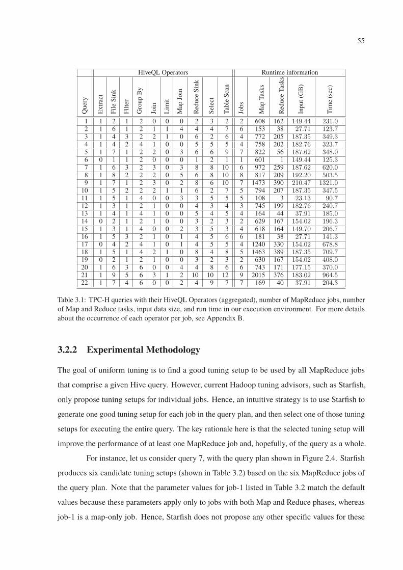
55

HiveQL Operators Runtime information

Quer

y

Extr

act

File

Sin

k

Filte

r

Gro

up

By

Join

Lim

it

Map

Join

Red

uce

Sin

k

Sel

ect

Tab

leSca

n

Jobs

Map

Tas

ks

Red

uce

Tas

ks

Input(G

B)

Tim

e(s

ec)

1 1 2 1 2 0 0 0 2 3 2 2 608 162 149.44 231.02 1 6 1 2 1 1 4 4 4 7 6 153 38 27.71 123.73 1 4 3 2 2 1 0 6 2 6 4 772 205 187.35 349.34 1 4 2 4 1 0 0 5 5 5 4 758 202 182.76 323.75 1 7 1 2 2 0 3 6 6 9 7 822 56 187.62 348.06 0 1 1 2 0 0 0 1 2 1 1 601 1 149.44 125.37 1 6 3 2 3 0 3 8 8 10 6 972 259 187.62 620.08 1 8 2 2 2 0 5 6 8 10 8 817 209 192.20 503.59 1 7 1 2 3 0 2 8 6 10 7 1473 390 210.47 1321.0

10 1 5 2 2 2 1 1 6 2 7 5 794 207 187.35 347.511 1 5 1 4 0 0 3 3 5 5 5 108 3 23.13 90.712 1 3 1 2 1 0 0 4 3 4 3 745 199 182.76 240.713 1 4 1 4 1 0 0 5 4 5 4 164 44 37.91 185.014 0 2 1 2 1 0 0 3 2 3 2 629 167 154.02 196.315 1 3 1 4 0 0 2 3 5 3 4 618 164 149.70 206.716 1 5 3 2 1 0 1 4 5 6 6 181 38 27.71 141.317 0 4 2 4 1 0 1 4 5 5 4 1240 330 154.02 678.818 1 5 1 4 2 1 0 8 4 8 5 1463 389 187.35 709.719 0 2 1 2 1 0 0 3 2 3 2 630 167 154.02 408.020 1 6 3 6 0 0 4 4 8 6 6 743 171 177.15 370.021 1 9 5 6 3 1 2 10 10 12 9 2015 376 183.02 964.522 1 7 4 6 0 0 2 4 9 7 7 169 40 37.91 204.3

Table 3.1: TPC-H queries with their HiveQL Operators (aggregated), number of MapReduce jobs, number

of Map and Reduce tasks, input data size, and run time in our execution environment. For more details

about the occurrence of each operator per job, see Appendix B.

3.2.2 Experimental Methodology

The goal of uniform tuning is to find a good tuning setup to be used by all MapReduce jobs

that comprise a given Hive query. However, current Hadoop tuning advisors, such as Starfish,

only propose tuning setups for individual jobs. Hence, an intuitive strategy is to use Starfish to

generate one good tuning setup for each job in the query plan, and then select one of those tuning

setups for executing the entire query. The key rationale here is that the selected tuning setup will

improve the performance of at least one MapReduce job and, hopefully, of the query as a whole.

For instance, let us consider query 7, with the query plan shown in Figure 2.4. Starfish

produces six candidate tuning setups (shown in Table 3.2) based on the six MapReduce jobs of

the query plan. Note that the parameter values for job-1 listed in Table 3.2 match the default

values because these parameters apply only to jobs with both Map and Reduce phases, whereas

job-1 is a map-only job. Hence, Starfish does not propose any other specific values for these

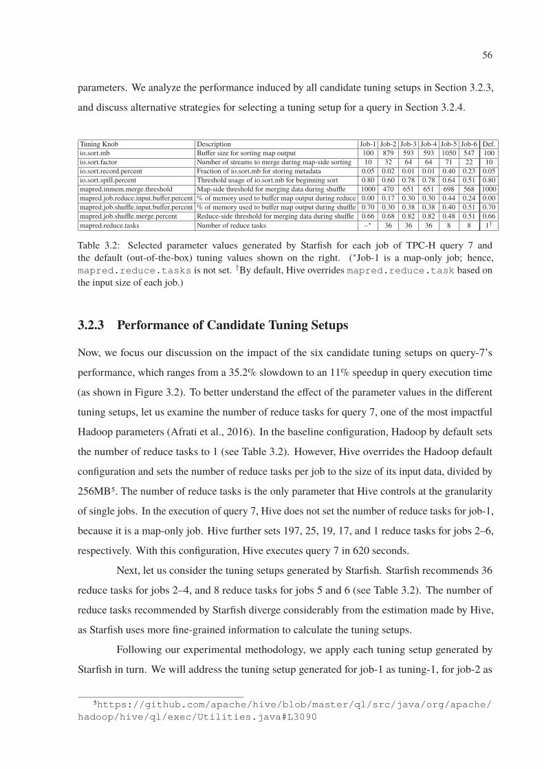
56

parameters. We analyze the performance induced by all candidate tuning setups in Section 3.2.3,

and discuss alternative strategies for selecting a tuning setup for a query in Section 3.2.4.

Tuning Knob Description Job-1 Job-2 Job-3 Job-4 Job-5 Job-6 Def.

io.sort.mb Buffer size for sorting map output 100 879 593 593 1050 547 100

io.sort.factor Number of streams to merge during map-side sorting 10 32 64 64 71 22 10

io.sort.record.percent Fraction of io.sort.mb for storing metadata 0.05 0.02 0.01 0.01 0.40 0.23 0.05

io.sort.spill.percent Threshold usage of io.sort.mb for beginning sort 0.80 0.60 0.78 0.78 0.64 0.51 0.80

mapred.inmem.merge.threshold Map-side threshold for merging data during shuffle 1000 470 651 651 698 568 1000

mapred.job.reduce.input.buffer.percent % of memory used to buffer map output during reduce 0.00 0.17 0.30 0.30 0.44 0.24 0.00

mapred.job.shuffle.input.buffer.percent % of memory used to buffer map output during shuffle 0.70 0.30 0.38 0.38 0.40 0.51 0.70

mapred.job.shuffle.merge.percent Reduce-side threshold for merging data during shuffle 0.66 0.68 0.82 0.82 0.48 0.51 0.66

mapred.reduce.tasks Number of reduce tasks –∗ 36 36 36 8 8 1†

Table 3.2: Selected parameter values generated by Starfish for each job of TPC-H query 7 and

the default (out-of-the-box) tuning values shown on the right. (∗Job-1 is a map-only job; hence,

mapred.reduce.tasks is not set. †By default, Hive overrides mapred.reduce.task based on

the input size of each job.)

3.2.3 Performance of Candidate Tuning Setups

Now, we focus our discussion on the impact of the six candidate tuning setups on query-7’s

performance, which ranges from a 35.2% slowdown to an 11% speedup in query execution time

(as shown in Figure 3.2). To better understand the effect of the parameter values in the different

tuning setups, let us examine the number of reduce tasks for query 7, one of the most impactful

Hadoop parameters (Afrati et al., 2016). In the baseline configuration, Hadoop by default sets

the number of reduce tasks to 1 (see Table 3.2). However, Hive overrides the Hadoop default

configuration and sets the number of reduce tasks per job to the size of its input data, divided by

256MB5. The number of reduce tasks is the only parameter that Hive controls at the granularity

of single jobs. In the execution of query 7, Hive does not set the number of reduce tasks for job-1,

because it is a map-only job. Hive further sets 197, 25, 19, 17, and 1 reduce tasks for jobs 2–6,

respectively. With this configuration, Hive executes query 7 in 620 seconds.

Next, let us consider the tuning setups generated by Starfish. Starfish recommends 36

reduce tasks for jobs 2–4, and 8 reduce tasks for jobs 5 and 6 (see Table 3.2). The number of

reduce tasks recommended by Starfish diverge considerably from the estimation made by Hive,

as Starfish uses more fine-grained information to calculate the tuning setups.

Following our experimental methodology, we apply each tuning setup generated by

Starfish in turn. We will address the tuning setup generated for job-1 as tuning-1, for job-2 as

5https://github.com/apache/hive/blob/master/ql/src/java/org/apache/hadoop/hive/ql/exec/Utilities.java#L3090

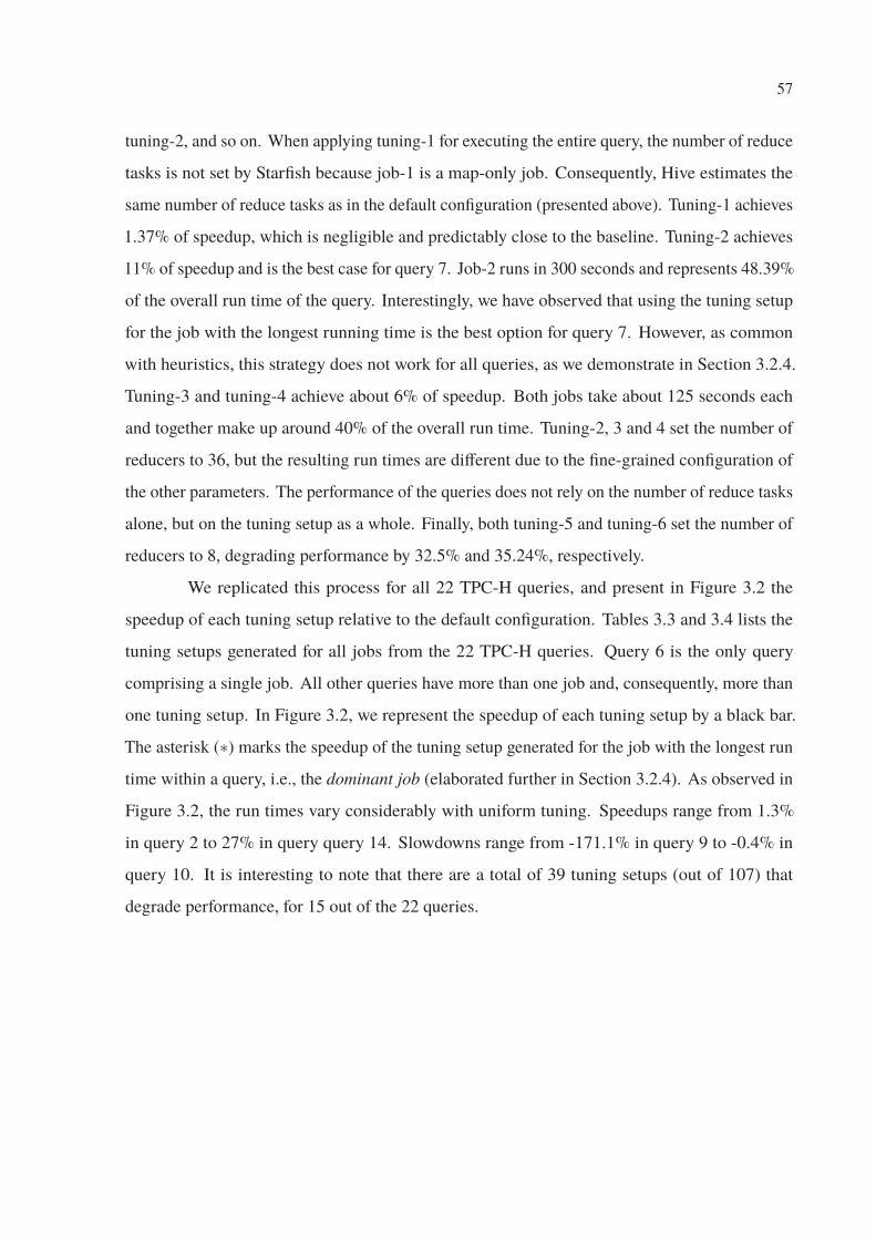
57

tuning-2, and so on. When applying tuning-1 for executing the entire query, the number of reduce

tasks is not set by Starfish because job-1 is a map-only job. Consequently, Hive estimates the

same number of reduce tasks as in the default configuration (presented above). Tuning-1 achieves

1.37% of speedup, which is negligible and predictably close to the baseline. Tuning-2 achieves

11% of speedup and is the best case for query 7. Job-2 runs in 300 seconds and represents 48.39%

of the overall run time of the query. Interestingly, we have observed that using the tuning setup

for the job with the longest running time is the best option for query 7. However, as common

with heuristics, this strategy does not work for all queries, as we demonstrate in Section 3.2.4.

Tuning-3 and tuning-4 achieve about 6% of speedup. Both jobs take about 125 seconds each

and together make up around 40% of the overall run time. Tuning-2, 3 and 4 set the number of

reducers to 36, but the resulting run times are different due to the fine-grained configuration of

the other parameters. The performance of the queries does not rely on the number of reduce tasks

alone, but on the tuning setup as a whole. Finally, both tuning-5 and tuning-6 set the number of

reducers to 8, degrading performance by 32.5% and 35.24%, respectively.

We replicated this process for all 22 TPC-H queries, and present in Figure 3.2 the

speedup of each tuning setup relative to the default configuration. Tables 3.3 and 3.4 lists the

tuning setups generated for all jobs from the 22 TPC-H queries. Query 6 is the only query

comprising a single job. All other queries have more than one job and, consequently, more than

one tuning setup. In Figure 3.2, we represent the speedup of each tuning setup by a black bar.

The asterisk (∗) marks the speedup of the tuning setup generated for the job with the longest run

time within a query, i.e., the dominant job (elaborated further in Section 3.2.4). As observed in

Figure 3.2, the run times vary considerably with uniform tuning. Speedups range from 1.3%

in query 2 to 27% in query query 14. Slowdowns range from -171.1% in query 9 to -0.4% in

query 10. It is interesting to note that there are a total of 39 tuning setups (out of 107) that

degrade performance, for 15 out of the 22 queries.

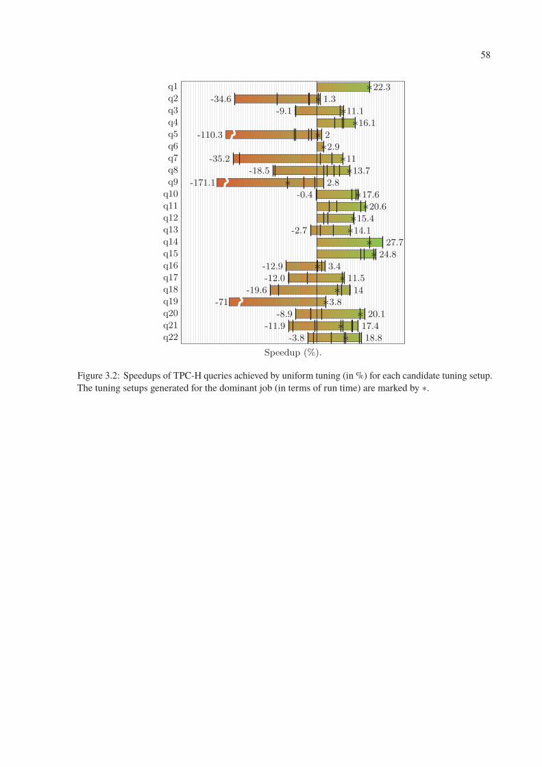
58

∗∗

∗∗

∗∗

∗∗

∗∗

∗∗∗

∗∗

∗∗

∗∗

∗∗∗

Figure 3.2: Speedups of TPC-H queries achieved by uniform tuning (in %) for each candidate tuning setup.

The tuning setups generated for the dominant job (in terms of run time) are marked by ∗.

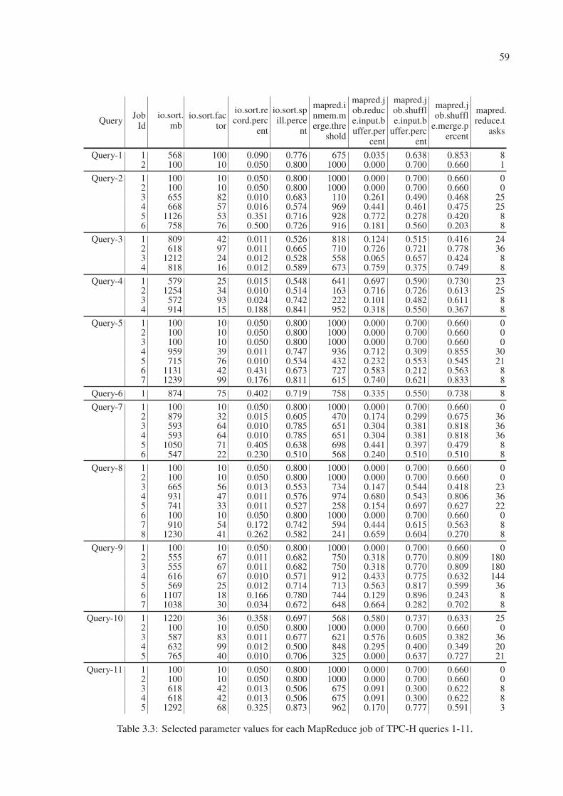
59

QueryJobId

io.sort.mb

io.sort.factor

io.sort.record.perc

ent

io.sort.spill.perce

nt

mapred.inmem.merge.thre

shold

mapred.job.reduce.input.buffer.per

cent

mapred.job.shuffle.input.b

uffer.percent

mapred.job.shuffl

e.merge.percent

mapred.reduce.t

asks

Query-1 1 568 100 0.090 0.776 675 0.035 0.638 0.853 82 100 10 0.050 0.800 1000 0.000 0.700 0.660 1

Query-2 1 100 10 0.050 0.800 1000 0.000 0.700 0.660 02 100 10 0.050 0.800 1000 0.000 0.700 0.660 03 655 82 0.010 0.683 110 0.261 0.490 0.468 254 668 57 0.016 0.574 969 0.441 0.461 0.475 255 1126 53 0.351 0.716 928 0.772 0.278 0.420 86 758 76 0.500 0.726 916 0.181 0.560 0.203 8

Query-3 1 809 42 0.011 0.526 818 0.124 0.515 0.416 242 618 97 0.011 0.665 710 0.726 0.721 0.778 363 1212 24 0.012 0.528 558 0.065 0.657 0.424 84 818 16 0.012 0.589 673 0.759 0.375 0.749 8

Query-4 1 579 25 0.015 0.548 641 0.697 0.590 0.730 232 1254 34 0.010 0.514 163 0.716 0.726 0.613 253 572 93 0.024 0.742 222 0.101 0.482 0.611 84 914 15 0.188 0.841 952 0.318 0.550 0.367 8

Query-5 1 100 10 0.050 0.800 1000 0.000 0.700 0.660 02 100 10 0.050 0.800 1000 0.000 0.700 0.660 03 100 10 0.050 0.800 1000 0.000 0.700 0.660 04 959 39 0.011 0.747 936 0.712 0.309 0.855 305 715 76 0.010 0.534 432 0.232 0.553 0.545 216 1131 42 0.431 0.673 727 0.583 0.212 0.563 87 1239 99 0.176 0.811 615 0.740 0.621 0.833 8

Query-6 1 874 75 0.402 0.719 758 0.335 0.550 0.738 8

Query-7 1 100 10 0.050 0.800 1000 0.000 0.700 0.660 02 879 32 0.015 0.605 470 0.174 0.299 0.675 363 593 64 0.010 0.785 651 0.304 0.381 0.818 364 593 64 0.010 0.785 651 0.304 0.381 0.818 365 1050 71 0.405 0.638 698 0.441 0.397 0.479 86 547 22 0.230 0.510 568 0.240 0.510 0.510 8

Query-8 1 100 10 0.050 0.800 1000 0.000 0.700 0.660 02 100 10 0.050 0.800 1000 0.000 0.700 0.660 03 665 56 0.013 0.553 734 0.147 0.544 0.418 234 931 47 0.011 0.576 974 0.680 0.543 0.806 365 741 33 0.011 0.527 258 0.154 0.697 0.627 226 100 10 0.050 0.800 1000 0.000 0.700 0.660 07 910 54 0.172 0.742 594 0.444 0.615 0.563 88 1230 41 0.262 0.582 241 0.659 0.604 0.270 8

Query-9 1 100 10 0.050 0.800 1000 0.000 0.700 0.660 02 555 67 0.011 0.682 750 0.318 0.770 0.809 1803 555 67 0.011 0.682 750 0.318 0.770 0.809 1804 616 67 0.010 0.571 912 0.433 0.775 0.632 1445 569 25 0.012 0.714 713 0.563 0.817 0.599 366 1107 18 0.166 0.780 744 0.129 0.896 0.243 87 1038 30 0.034 0.672 648 0.664 0.282 0.702 8

Query-10 1 1220 36 0.358 0.697 568 0.580 0.737 0.633 252 100 10 0.050 0.800 1000 0.000 0.700 0.660 03 587 83 0.011 0.677 621 0.576 0.605 0.382 364 632 99 0.012 0.500 848 0.295 0.400 0.349 205 765 40 0.010 0.706 325 0.000 0.637 0.727 21

Query-11 1 100 10 0.050 0.800 1000 0.000 0.700 0.660 02 100 10 0.050 0.800 1000 0.000 0.700 0.660 03 618 42 0.013 0.506 675 0.091 0.300 0.622 84 618 42 0.013 0.506 675 0.091 0.300 0.622 85 1292 68 0.325 0.873 962 0.170 0.777 0.591 3

Table 3.3: Selected parameter values for each MapReduce job of TPC-H queries 1-11.

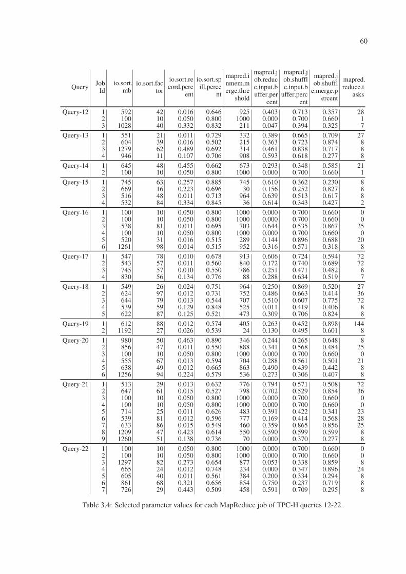
60

QueryJobId

io.sort.mb

io.sort.factor

io.sort.record.perc

ent

io.sort.spill.perce

nt

mapred.inmem.merge.thre

shold

mapred.job.reduce.input.buffer.per

cent

mapred.job.shuffle.input.b

uffer.percent

mapred.job.shuffl

e.merge.percent

mapred.reduce.t

asks

Query-12 1 592 42 0.016 0.646 925 0.403 0.713 0.357 282 100 10 0.050 0.800 1000 0.000 0.700 0.660 13 1028 40 0.332 0.832 211 0.047 0.394 0.325 7

Query-13 1 551 21 0.011 0.729 332 0.389 0.665 0.709 272 604 39 0.016 0.502 215 0.363 0.723 0.874 83 1279 62 0.489 0.692 314 0.461 0.838 0.717 84 946 11 0.107 0.706 908 0.593 0.618 0.277 8

Query-14 1 645 48 0.455 0.662 673 0.293 0.348 0.585 212 100 10 0.050 0.800 1000 0.000 0.700 0.660 1

Query-15 1 745 63 0.257 0.885 745 0.610 0.362 0.230 82 669 16 0.223 0.696 30 0.156 0.252 0.827 83 516 48 0.011 0.713 964 0.639 0.513 0.617 84 532 84 0.334 0.845 36 0.614 0.343 0.427 2

Query-16 1 100 10 0.050 0.800 1000 0.000 0.700 0.660 02 100 10 0.050 0.800 1000 0.000 0.700 0.660 03 538 81 0.011 0.695 703 0.644 0.535 0.867 254 100 10 0.050 0.800 1000 0.000 0.700 0.660 05 520 31 0.016 0.515 289 0.144 0.896 0.688 206 1261 98 0.014 0.515 952 0.316 0.571 0.318 8

Query-17 1 547 78 0.010 0.678 913 0.606 0.724 0.594 722 543 57 0.011 0.560 840 0.172 0.740 0.689 723 745 57 0.010 0.550 786 0.251 0.471 0.482 84 830 56 0.134 0.776 88 0.288 0.634 0.519 7

Query-18 1 549 26 0.024 0.751 964 0.250 0.869 0.520 272 624 97 0.012 0.731 752 0.486 0.663 0.414 363 644 79 0.013 0.544 707 0.510 0.607 0.775 724 539 59 0.129 0.848 525 0.011 0.419 0.406 85 622 87 0.125 0.521 473 0.309 0.706 0.824 8

Query-19 1 612 88 0.012 0.574 405 0.263 0.452 0.898 1442 1192 27 0.026 0.539 24 0.130 0.495 0.601 8

Query-20 1 980 50 0.463 0.890 346 0.244 0.265 0.648 82 856 47 0.011 0.550 888 0.341 0.568 0.484 253 100 10 0.050 0.800 1000 0.000 0.700 0.660 04 555 67 0.013 0.594 704 0.288 0.561 0.501 215 638 49 0.012 0.665 863 0.490 0.439 0.442 86 1256 94 0.224 0.579 536 0.273 0.306 0.407 8

Query-21 1 513 29 0.013 0.632 776 0.794 0.571 0.508 722 647 61 0.015 0.527 798 0.702 0.529 0.854 363 100 10 0.050 0.800 1000 0.000 0.700 0.660 04 100 10 0.050 0.800 1000 0.000 0.700 0.660 05 714 25 0.011 0.626 483 0.391 0.422 0.341 236 539 81 0.012 0.596 777 0.169 0.414 0.568 287 633 86 0.015 0.549 460 0.359 0.865 0.856 258 1209 47 0.423 0.614 550 0.590 0.599 0.599 89 1260 51 0.138 0.736 70 0.000 0.370 0.277 8

Query-22 1 100 10 0.050 0.800 1000 0.000 0.700 0.660 02 100 10 0.050 0.800 1000 0.000 0.700 0.660 03 1297 82 0.273 0.654 877 0.053 0.338 0.859 84 665 24 0.012 0.748 234 0.000 0.347 0.896 245 605 40 0.011 0.561 384 0.200 0.334 0.294 86 861 68 0.321 0.656 854 0.750 0.237 0.719 87 726 29 0.443 0.509 458 0.591 0.709 0.295 8

Table 3.4: Selected parameter values for each MapReduce job of TPC-H queries 12-22.

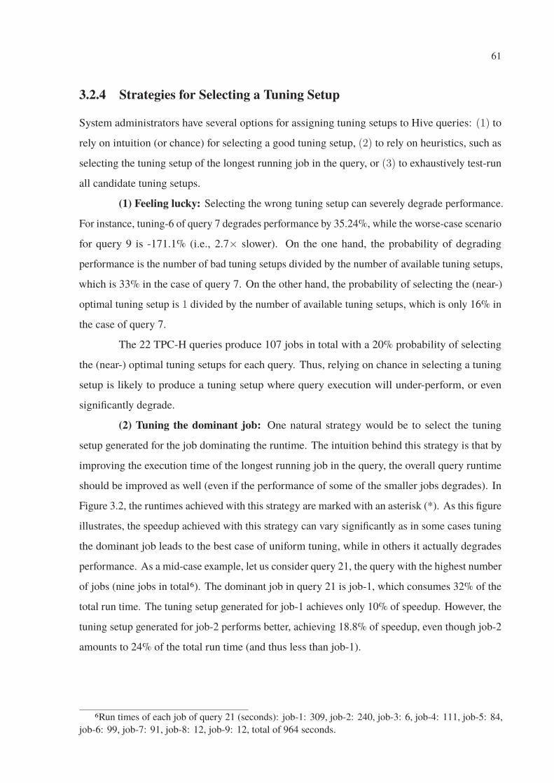
61

3.2.4 Strategies for Selecting a Tuning Setup

System administrators have several options for assigning tuning setups to Hive queries: (1) to

rely on intuition (or chance) for selecting a good tuning setup, (2) to rely on heuristics, such as

selecting the tuning setup of the longest running job in the query, or (3) to exhaustively test-run

all candidate tuning setups.

(1) Feeling lucky: Selecting the wrong tuning setup can severely degrade performance.

For instance, tuning-6 of query 7 degrades performance by 35.24%, while the worse-case scenario

for query 9 is -171.1% (i.e., 2.7× slower). On the one hand, the probability of degrading

performance is the number of bad tuning setups divided by the number of available tuning setups,

which is 33% in the case of query 7. On the other hand, the probability of selecting the (near-)

optimal tuning setup is 1 divided by the number of available tuning setups, which is only 16% in

the case of query 7.

The 22 TPC-H queries produce 107 jobs in total with a 20% probability of selecting

the (near-) optimal tuning setups for each query. Thus, relying on chance in selecting a tuning

setup is likely to produce a tuning setup where query execution will under-perform, or even

significantly degrade.

(2) Tuning the dominant job: One natural strategy would be to select the tuning

setup generated for the job dominating the runtime. The intuition behind this strategy is that by

improving the execution time of the longest running job in the query, the overall query runtime

should be improved as well (even if the performance of some of the smaller jobs degrades). In

Figure 3.2, the runtimes achieved with this strategy are marked with an asterisk (*). As this figure

illustrates, the speedup achieved with this strategy can vary significantly as in some cases tuning

the dominant job leads to the best case of uniform tuning, while in others it actually degrades

performance. As a mid-case example, let us consider query 21, the query with the highest number

of jobs (nine jobs in total6). The dominant job in query 21 is job-1, which consumes 32% of the

total run time. The tuning setup generated for job-1 achieves only 10% of speedup. However, the

tuning setup generated for job-2 performs better, achieving 18.8% of speedup, even though job-2

amounts to 24% of the total run time (and thus less than job-1).

6Run times of each job of query 21 (seconds): job-1: 309, job-2: 240, job-3: 6, job-4: 111, job-5: 84,

job-6: 99, job-7: 91, job-8: 12, job-9: 12, total of 964 seconds.

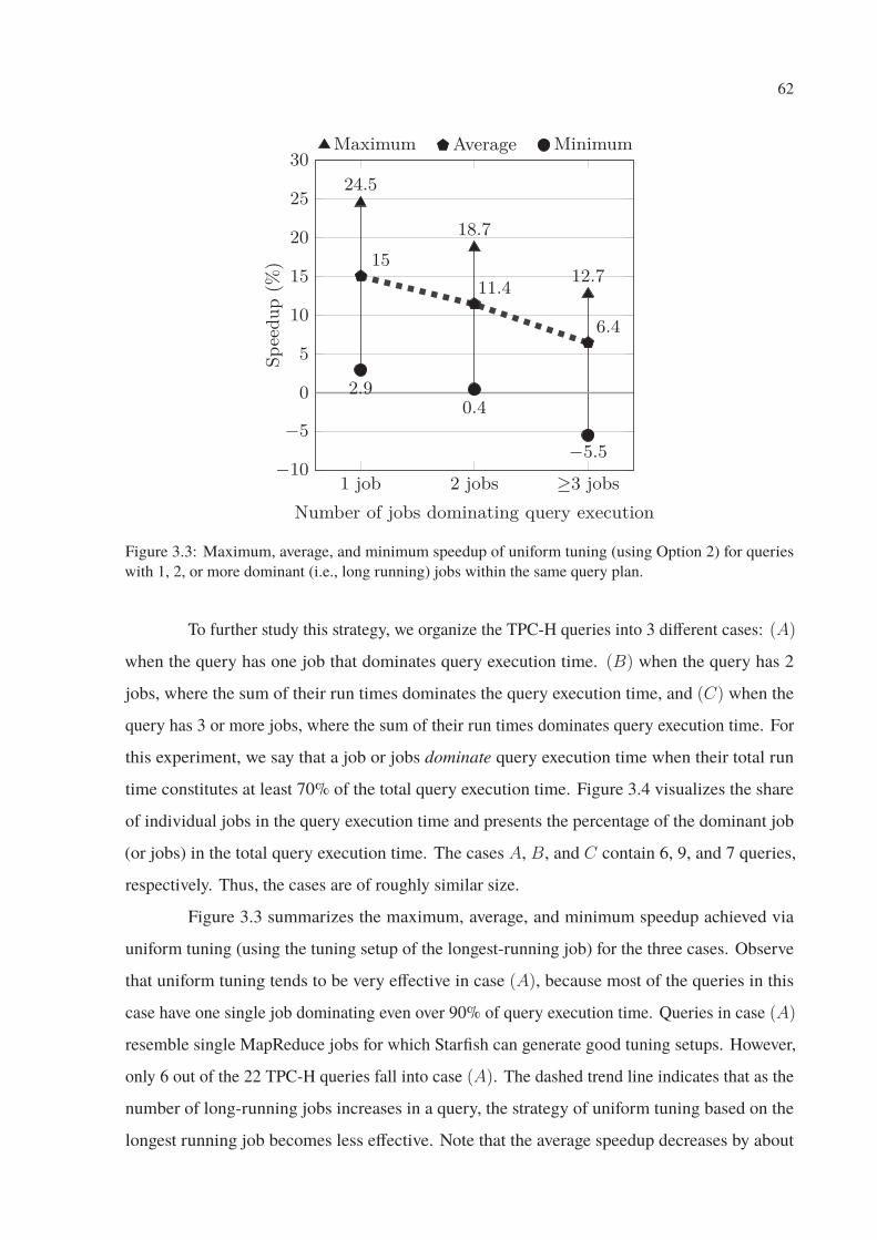
62

≥−10

−5

0

5

10

15

20

25

3024.5

18.7

12.715

11.4

6.4

2.90.4

−5.5

Figure 3.3: Maximum, average, and minimum speedup of uniform tuning (using Option 2) for queries

with 1, 2, or more dominant (i.e., long running) jobs within the same query plan.

To further study this strategy, we organize the TPC-H queries into 3 different cases: (A)

when the query has one job that dominates query execution time. (B) when the query has 2

jobs, where the sum of their run times dominates the query execution time, and (C) when the

query has 3 or more jobs, where the sum of their run times dominates query execution time. For

this experiment, we say that a job or jobs dominate query execution time when their total run

time constitutes at least 70% of the total query execution time. Figure 3.4 visualizes the share

of individual jobs in the query execution time and presents the percentage of the dominant job

(or jobs) in the total query execution time. The cases A, B, and C contain 6, 9, and 7 queries,

respectively. Thus, the cases are of roughly similar size.

Figure 3.3 summarizes the maximum, average, and minimum speedup achieved via

uniform tuning (using the tuning setup of the longest-running job) for the three cases. Observe

that uniform tuning tends to be very effective in case (A), because most of the queries in this

case have one single job dominating even over 90% of query execution time. Queries in case (A)

resemble single MapReduce jobs for which Starfish can generate good tuning setups. However,

only 6 out of the 22 TPC-H queries fall into case (A). The dashed trend line indicates that as the

number of long-running jobs increases in a query, the strategy of uniform tuning based on the

longest running job becomes less effective. Note that the average speedup decreases by about

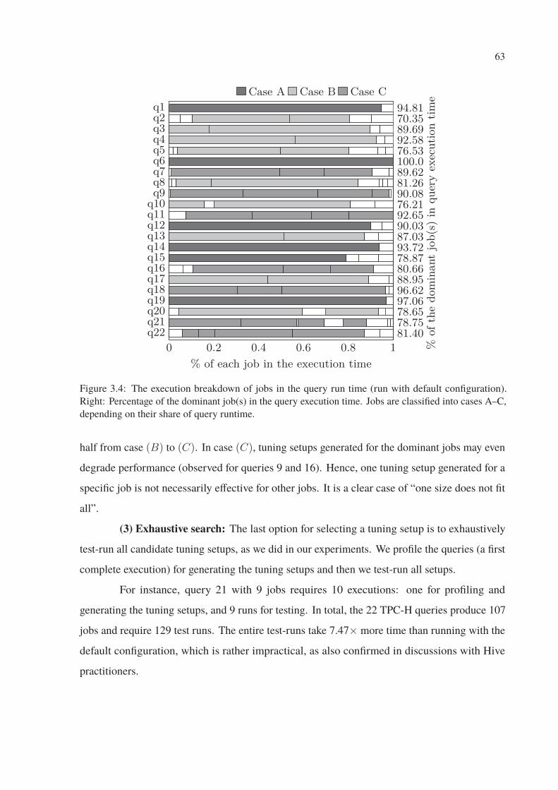
63

0 0.2 0.4 0.6 0.8 1

Figure 3.4: The execution breakdown of jobs in the query run time (run with default configuration).

Right: Percentage of the dominant job(s) in the query execution time. Jobs are classified into cases A–C,

depending on their share of query runtime.

half from case (B) to (C). In case (C), tuning setups generated for the dominant jobs may even

degrade performance (observed for queries 9 and 16). Hence, one tuning setup generated for a

specific job is not necessarily effective for other jobs. It is a clear case of “one size does not fit

all”.

(3) Exhaustive search: The last option for selecting a tuning setup is to exhaustively

test-run all candidate tuning setups, as we did in our experiments. We profile the queries (a first

complete execution) for generating the tuning setups and then we test-run all setups.

For instance, query 21 with 9 jobs requires 10 executions: one for profiling and

generating the tuning setups, and 9 runs for testing. In total, the 22 TPC-H queries produce 107

jobs and require 129 test runs. The entire test-runs take 7.47× more time than running with the

default configuration, which is rather impractical, as also confirmed in discussions with Hive

practitioners.

64

3.3 Discussion

The current approach for tuning SQL-on-Hadoop queries relies on replicating the same tuning

setup to all jobs in the query plan. This leads to the problem of finding the best tuning setup that

benefits the query plan as a whole when replicated. Finding the best tuning might be impossible

due to the different characteristics of each job, once they implement a different mix of relational

algebra operators.

Current strategies for selecting this tuning setup can be very expensive (like exhaustive

search where we test-run all tuning candidates), or based on heuristics (like tuning the dominant

resource consumption job). When tuning for dominant jobs, we observe that tuning queries with

tuning setups of dominant jobs can speed up run time for queries with 1 or 2 dominant jobs.

However, tuning setups of dominant jobs begin to lose their effectiveness when the execution

time is equally distributed by 3 or more jobs, as presented in Figure 3.3. For instance, from

the 22 TPC-H queries, tuning the dominant jobs can speed up 70% of the queries. Yet, further

analysis is required to determine whether different workloads present the same distribution of

dominant jobs.

Tuning SQL-on-Hadoop queries require a large amount of manual work to test-run

available tuning alternatives. Test-run all alternatives is time consuming, for instance, it takes

7.47× to test-run all tuning alternatives for TPC-H. Even after testing all available alternatives,

there is no guarantee that the chosen tuning setup is optimal. And after a tuning setup is

chosen, Hive forbids users to apply tuning setups in a job-basis, which also drives to sub-optimal

performance. In the next Chapter, we present our alternative approach to automatically tune

SQL-on-Hadoop queries in a job-basis as an extension of Hive.

We validated our approach with the TPC-H benchmark, which is a decision support

benchmark that examines large volumes of data and consists of 22 ad-hoc queries. These queries

have broad industry relevance and are extensively used by the database community.

65

Chapter 4

Intra-Query Physical-Layer Tuning

In this Chapter, we present the non-uniform tuning approach as an alternative to uniform tuning:

Each MapReduce job in a HiveQL query is executed with its own tuning setup. We also present

the impact of non-uniform tuning on query execution run time, and compare both approaches.

4.1 The Non-Uniform Tuning Approach

For a query plan G = (V,E), there are jobs that implement different sets of SQL operators, i.e.,

there are jobs u, v ∈ V where we have Ou �= Ov. Consequently, we assume that these jobs have

different resource consumption needs (Boncz et al., 2013). The resource consumption of the 22

TPC-H queries, running with default configuration, is listed in Appendix A. For instance, while

a job u requires disk bandwidth due to a TableScan operator, another job v requires memory

throughput due to a Sort operator. One job of a query plan may implement multiple algebra

operators due to MapReduce optimization techniques like chain folding and job merging. In this

case, the resource consumption requirements are more complex than of single TableScan or Sort

operators.

Thus, the optimum of the SQL-on-Hadoop Tuning Problem, presented in Equation 3.3,

can only be found when tuning each job of the query plan with appropriate tuning setups. We

name this approach as Non-Uniform Tuning, and define it as follows:

Definition 4 (Non-Uniform Tuning): The Non-Uniform Tuning approach is the assignment of

different configurations to jobs such that Cu �= Cv for any u, v ∈ V that has Ou �= Ov.

We observed in our experiments that there are cases where, in the same query plan,

different jobs implement the same set of query operators. In these cases, the same tuning setup

66

can be applied, although the behavior of such jobs might differ due to the distribution of the data,

selectivity and similar aspects. We discuss these cases in Section 5.1.

Next, we compare the performance of the Uniform and Non-Uniform tuning approaches.

4.2 Performance of Non-Uniform Tuning

Claim 1: Considering C ′, from Definition 2, the Non-Uniform tuning approach, performs better

than the Uniform tuning, or equal, in the worst-case.

Consider that Cu is the tuning setup generated for job u, for u ∈ V . Let Cu be assigned

using the uniform tuning, i.e., be the tuning setup assigned to all jobs v ∈ V . Now, consider

the case with non-uniform tuning, in which for the same query plan G, the most efficient tuning

for every job v can be naively obtained by calling interactively the function f(v). Directly from

Definition 3.1 we have the following inequality

σ(v, f(v)) ≤ σ(v, Cu) (4.1)

for every job v ∈ V .

The inequality says that, in the best case for the uniform tuning, the arbitrary tuning

setup Cu can be the most efficient for v, but there are no guarantees that it will happen. While

attributing a tuning setup Cv chosen by the function f(v), we know that it is always the optimal

tuning setup for v. Consequently, the total cost required to execute all jobs v ∈ V of the query

plan G using the adviser function, can be written as Equation 3.2. So, from the inequality (4.1)

we can compare the total costs of the two approaches, as follows:

∑v∈V

σ(v, f(v)) ≤∑v∈V

σ(v, Cu),

i.e., the computational cost for executing the query plan G using the non-uniform assignment

method is at most equals to the cost for the uniform method. However, we know Equation 3.2

67

is the naive approach that generates sub-optimal solution for tuning a query plan, and that the

optimal solution is found by Definition 3, such that,

∑Cv∈C′

σ(v, Cv) ≤∑v∈V

σ(v, f(v)) ≤∑v∈V

σ(v, Cu) (4.2)

The advantage of using the uniform tuning method is that it is simple and straightforward,

i.e., the SQL-on-Hadoop engine just replicates the chosen tuning setup. On the other hand, there

are no guarantees that the chosen tuning setup will perform well during the query’s execution.

Our proposal of non-uniform tuning personalizes the tuning setup for each job and

the optimal assignment of tuning setups is guaranteed. In other words, the SQL-on-Hadoop’s

Tuning Problem can be solved optimally with the Non-Uniform tuning method. Furthermore, a

direct consequence of the Non-Uniform tuning approach is the improvement in the performance

of the query plan, as stated in Claim 1.

4.3 Cost of the Non-Uniform Tuning

Denoting Cv as the configuration for a vertex v ∈ V and considering that every tuning parameter

ci of the configuration Cv has a different domain dom(ci) of size di. The computational cost for

the worst case of finding an optimal solution for the non-uniform tuning can be stated as follows.

Theorem 1: The cost of finding the optimal Non-Uniform tuning for a query plan G = (V,E),

is of O(|V |nm), where n = max1≤i≤m{di},m = |Cv|.

Proof 1: We can enumerate all possible configurations for a single v by the following product:

m∏i=1

di.

Since different domains have different sizes (including infinite domains), let the max size for a

parameter domain be n = max1≤i≤m{di}. An upper bound for such product is

m∏i=1

di ≤m∏i=1

n = nm

68

Thus, it is required time O(nm) to find the optimal configuration for a job v. Consider that we

want to find the optimal configuration for every vertex v ∈ V , that is,

∏v∈V

O(nm), (4.3)

therefore, we need time O(nm|V |) for the whole graph G.

�

Similarly, the cost of finding the optimal configuration for the uniform tuning is O(nm),

since we need to find only one optimal configuration C0 which is propagated to the entire graph.

4.4 Non-Uniform Tuning Methodology

As of today, there is no mechanism in Hive for applying tuning setups at the level of individual

jobs within the same query plan, even though MapReduce jobs can be configured individually

when submitted separately. We therefore extended the Hive query processing engine to switch

between tuning setups, executing each job with its own tuning setup. Our extension does not

change the current query processing workflow, described in Section 2.5. Instead, our extension

just rewrites the configuration of every job right before it is queued in Hadoop for processing. Our

fork of Hive is fully functional, to the point where a Hive administrator can enable our extension

by merely setting a single, new parameter (hive.optimize.selftuning) to true.

We run the TPC-H queries with our extension to analyze the performance impact of

non-uniform tuning. For instance, let us consider TPC-H query 7 again. When the query is

submitted, it is processed and optimized by the Hive query processing engine: All its jobs have

been created and all Hive optimizations have been performed with the query plan looking as

depicted in Figure 2.4. At this point, our extension calls Starfish to profile and optimize every job

of query 7 (recall Section 2.4), and stores the recommended tuning setups in a cache repository.

The cache repository is presented in Section 5.1. Briefly, the cache associates the code

signature of each job with its recommended tuning setup. A code signature is a set of annotations

generated during query compilation that capture the query operators executed as part of a job,

along with some basic data properties (similar to the information contained in Figure 2.4). The

code signature can be used to uniquely identify a job within the same query plan. When query 7

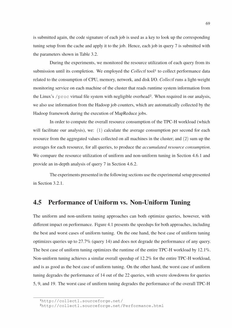
69

is submitted again, the code signature of each job is used as a key to look up the corresponding

tuning setup from the cache and apply it to the job. Hence, each job in query 7 is submitted with

the parameters shown in Table 3.2.

During the experiments, we monitored the resource utilization of each query from its

submission until its completion. We employed the Collectl tool1 to collect performance data

related to the consumption of CPU, memory, network, and disk I/O. Collectl runs a light-weight

monitoring service on each machine of the cluster that reads runtime system information from

the Linux’s /proc virtual file system with negligible overhead2. When required in our analysis,

we also use information from the Hadoop job counters, which are automatically collected by the

Hadoop framework during the execution of MapReduce jobs.

In order to compute the overall resource consumption of the TPC-H workload (which

will facilitate our analysis), we: (1) calculate the average consumption per second for each

resource from the aggregated values collected on all machines in the cluster; and (2) sum up the

averages for each resource, for all queries, to produce the accumulated resource consumption.

We compare the resource utilization of uniform and non-uniform tuning in Section 4.6.1 and

provide an in-depth analysis of query 7 in Section 4.6.2.

The experiments presented in the following sections use the experimental setup presented

in Section 3.2.1.

4.5 Performance of Uniform vs. Non-Uniform Tuning

The uniform and non-uniform tuning approaches can both optimize queries, however, with

different impact on performance. Figure 4.1 presents the speedups for both approaches, including

the best and worst cases of uniform tuning. On the one hand, the best case of uniform tuning

optimizes queries up to 27.7% (query 14) and does not degrade the performance of any query.

The best case of uniform tuning optimizes the runtime of the entire TPC-H workload by 12.1%.

Non-uniform tuning achieves a similar overall speedup of 12.2% for the entire TPC-H workload,

and is as good as the best case of uniform tuning. On the other hand, the worst case of uniform

tuning degrades the performance of 14 out of the 22 queries, with severe slowdowns for queries

5, 9, and 19. The worst case of uniform tuning degrades the performance of the overall TPC-H

1http://collectl.sourceforge.net/2http://collectl.sourceforge.net/Performance.html

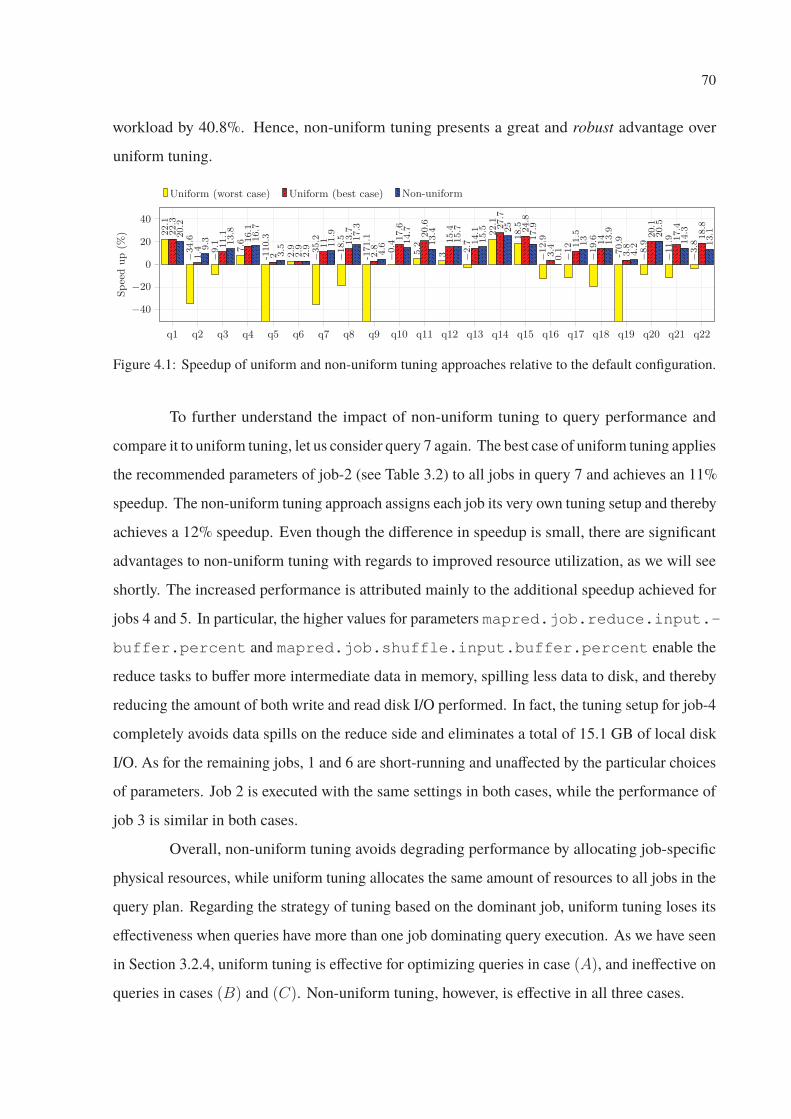
70

workload by 40.8%. Hence, non-uniform tuning presents a great and robust advantage over

uniform tuning.

−40

−20

0

20

40

22.1

−34.

6

−9.1 7.6

2.9

−35.

2

−18.

5

−0.4

5.2

3 −2.7

22.1

18.5

−12.

9

−12

−19.

6

−8.9

−11.

9

−3.8

22.3

1.4 11

.1 16.1

2 2.9 11 13

.7

2.8

17.6 20.6

15.4

14.1 27

.7

24.8

3.4 11

.5

14

3.8

20.1

17.4

18.8

20.2

9.3 13

.8 16.7

3.5

2.9 11

.9 17.3

4.6 14

.7

13.4

15.7

15.5 25

17.9

0.1

13 13.9

4.2

20.5

14.3

13.1

Figure 4.1: Speedup of uniform and non-uniform tuning approaches relative to the default configuration.

To further understand the impact of non-uniform tuning to query performance and

compare it to uniform tuning, let us consider query 7 again. The best case of uniform tuning applies

the recommended parameters of job-2 (see Table 3.2) to all jobs in query 7 and achieves an 11%

speedup. The non-uniform tuning approach assigns each job its very own tuning setup and thereby

achieves a 12% speedup. Even though the difference in speedup is small, there are significant

advantages to non-uniform tuning with regards to improved resource utilization, as we will see

shortly. The increased performance is attributed mainly to the additional speedup achieved for

jobs 4 and 5. In particular, the higher values for parameters mapred.job.reduce.input.-

buffer.percent and mapred.job.shuffle.input.buffer.percent enable the

reduce tasks to buffer more intermediate data in memory, spilling less data to disk, and thereby

reducing the amount of both write and read disk I/O performed. In fact, the tuning setup for job-4

completely avoids data spills on the reduce side and eliminates a total of 15.1 GB of local disk

I/O. As for the remaining jobs, 1 and 6 are short-running and unaffected by the particular choices

of parameters. Job 2 is executed with the same settings in both cases, while the performance of

job 3 is similar in both cases.

Overall, non-uniform tuning avoids degrading performance by allocating job-specific

physical resources, while uniform tuning allocates the same amount of resources to all jobs in the

query plan. Regarding the strategy of tuning based on the dominant job, uniform tuning loses its

effectiveness when queries have more than one job dominating query execution. As we have seen

in Section 3.2.4, uniform tuning is effective for optimizing queries in case (A), and ineffective on

queries in cases (B) and (C). Non-uniform tuning, however, is effective in all three cases.

71

Another advantage of non-uniform tuning is the self-tuning nature of the approach.

Human intervention becomes impractical when any ordinary OLAP workload generates tens to

hundreds of jobs and many more possible tuning setups.

In our experiments, optimizing each job individually in non-uniform tuning always leads

to better performance results but not always the best. As we can observe from Figure 4.1, the

best-case of uniform approach is a little better (0.1–7.2% higher speedup) than the non-uniform

one for 9 out of the 22 TPC-H queries. There are two main reasons for this behavior. First, almost

all Hadoop tuning advisors (including Starfish) treat the Map and Reduce functions as black

boxes and make simplifying modeling assumptions. For example, some make the proportionality

assumption (Herodotou and Babu, 2011), based on which the execution time of a function will

double if its input size is doubled. This assumption may hold for simple jobs like WordCount or

Sort, but it is not true for jobs that contain multiple relational algebra operators like joins and

aggregators. Hence, the modeling, and consequently the tuning recommendations, might not

be optimal. Second, performance dependencies between jobs complicate the task of a tuning

advisor. For example, setting the number of Reduce tasks or enabling output compression for

one MapReduce job will affect the performance of the subsequent job as it will affect the number

of Map tasks and the need for decompression for the second job, respectively. Hence, it is harder

to generate optimal tuning setups for later jobs in a query execution plan. Overall, there is a

dire need for (1) better modeling techniques when the MapReduce jobs are generated by the

query compilers of SQL-on-Hadoop systems, especially since there is inside knowledge of which

operations the jobs will perform, and (2) better optimizers that can take into consideration the

interdependencies of jobs and holistically optimize the entire workflow.

4.6 Impact on Resource Utilization

Apart from execution time speedup, Hadoop parameter tuning can have a significant impact on

the physical resources that are consumed during the execution of HiveQL queries. In this section,

we study and compare the impact of uniform and non-uniform tuning on resource utilization.

4.6.1 Resource Utilization of Uniform vs. Non-uniform Tuning

Figure 4.2 depicts the relative percentage of the accumulated resource consumption of the

TPC-H workload running with uniform and non-uniform tuning, compared against the default

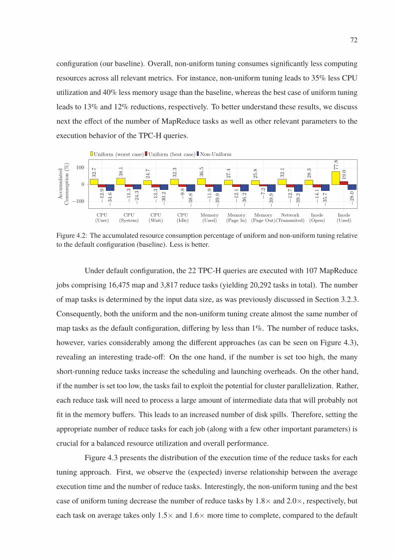
72

configuration (our baseline). Overall, non-uniform tuning consumes significantly less computing

resources across all relevant metrics. For instance, non-uniform tuning leads to 35% less CPU

utilization and 40% less memory usage than the baseline, whereas the best case of uniform tuning

leads to 13% and 12% reductions, respectively. To better understand these results, we discuss

next the effect of the number of MapReduce tasks as well as other relevant parameters to the

execution behavior of the TPC-H queries.

−100

0

100

32.7

38.1

24.7

32.3

36.5

27.4

25.8

32.1

28.3 77

.8

−12.

9

−11.

3

−13.

3

−9.8

−11.

9

−12.

1

−7.2

−12.

7

−14.

1

19.0

−34.

6

−24.

3

−30.

2

−38.

8

−39.

9

−36.

2

−39.

9

−39.

2

−35.

7

−28.

0

Figure 4.2: The accumulated resource consumption percentage of uniform and non-uniform tuning relative

to the default configuration (baseline). Less is better.

Under default configuration, the 22 TPC-H queries are executed with 107 MapReduce

jobs comprising 16,475 map and 3,817 reduce tasks (yielding 20,292 tasks in total). The number

of map tasks is determined by the input data size, as was previously discussed in Section 3.2.3.

Consequently, both the uniform and the non-uniform tuning create almost the same number of

map tasks as the default configuration, differing by less than 1%. The number of reduce tasks,

however, varies considerably among the different approaches (as can be seen on Figure 4.3),

revealing an interesting trade-off: On the one hand, if the number is set too high, the many

short-running reduce tasks increase the scheduling and launching overheads. On the other hand,

if the number is set too low, the tasks fail to exploit the potential for cluster parallelization. Rather,

each reduce task will need to process a large amount of intermediate data that will probably not

fit in the memory buffers. This leads to an increased number of disk spills. Therefore, setting the

appropriate number of reduce tasks for each job (along with a few other important parameters) is

crucial for a balanced resource utilization and overall performance.

Figure 4.3 presents the distribution of the execution time of the reduce tasks for each

tuning approach. First, we observe the (expected) inverse relationship between the average

execution time and the number of reduce tasks. Interestingly, the non-uniform tuning and the best

case of uniform tuning decrease the number of reduce tasks by 1.8× and 2.0×, respectively, but

each task on average takes only 1.5× and 1.6× more time to complete, compared to the default

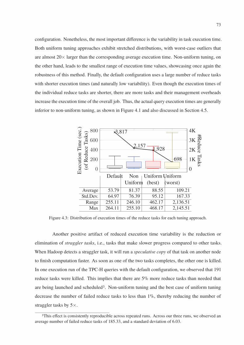
73

configuration. Nonetheless, the most important difference is the variability in task execution time.

Both uniform tuning approaches exhibit stretched distributions, with worst-case outliers that

are almost 20× larger than the corresponding average execution time. Non-uniform tuning, on

the other hand, leads to the smallest range of execution time values, showcasing once again the

robustness of this method. Finally, the default configuration uses a large number of reduce tasks

with shorter execution times (and naturally low variability). Even though the execution times of

the individual reduce tasks are shorter, there are more tasks and their management overheads

increase the execution time of the overall job. Thus, the actual query execution times are generally

inferior to non-uniform tuning, as shown in Figure 4.1 and also discussed in Section 4.5.

Default Non

Uniform

Uniform

(best)

Uniform

(worst)

0

200

400

600

800

0

1K

2K

3K

4K3,817

2,1571,928

698

Exec

ution

Tim

e(s

ec.)

(of

Red

uce

Tas

ks) #

Red

uce

Task

s

Average 53.79 81.37 88.55 109.21

Std.Dev. 64.97 76.39 95.12 167.33

Range 255.11 246.10 462.17 2,136.51

Max 264.11 255.10 468.17 2,145.51

Figure 4.3: Distribution of execution times of the reduce tasks for each tuning approach.

Another positive artifact of reduced execution time variability is the reduction or

elimination of straggler tasks, i.e., tasks that make slower progress compared to other tasks.

When Hadoop detects a straggler task, it will run a speculative copy of that task on another node

to finish computation faster. As soon as one of the two tasks completes, the other one is killed.

In one execution run of the TPC-H queries with the default configuration, we observed that 191

reduce tasks were killed. This implies that there are 5% more reduce tasks than needed that

are being launched and scheduled3. Non-uniform tuning and the best case of uniform tuning

decrease the number of failed reduce tasks to less than 1%, thereby reducing the number of

straggler tasks by 5×.

3This effect is consistently reproducible across repeated runs. Across our three runs, we observed an

average number of failed reduce tasks of 185.33, and a standard deviation of 6.03.

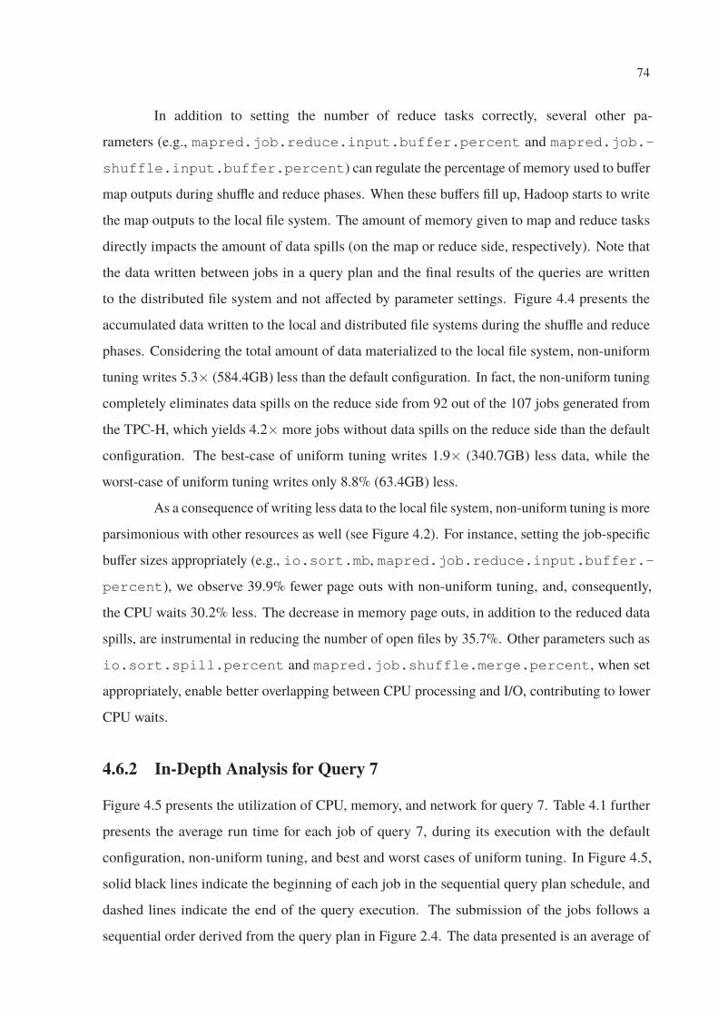
74

In addition to setting the number of reduce tasks correctly, several other pa-

rameters (e.g., mapred.job.reduce.input.buffer.percent and mapred.job.-

shuffle.input.buffer.percent) can regulate the percentage of memory used to buffer

map outputs during shuffle and reduce phases. When these buffers fill up, Hadoop starts to write

the map outputs to the local file system. The amount of memory given to map and reduce tasks

directly impacts the amount of data spills (on the map or reduce side, respectively). Note that

the data written between jobs in a query plan and the final results of the queries are written

to the distributed file system and not affected by parameter settings. Figure 4.4 presents the

accumulated data written to the local and distributed file systems during the shuffle and reduce

phases. Considering the total amount of data materialized to the local file system, non-uniform

tuning writes 5.3× (584.4GB) less than the default configuration. In fact, the non-uniform tuning

completely eliminates data spills on the reduce side from 92 out of the 107 jobs generated from

the TPC-H, which yields 4.2× more jobs without data spills on the reduce side than the default

configuration. The best-case of uniform tuning writes 1.9× (340.7GB) less data, while the

worst-case of uniform tuning writes only 8.8% (63.4GB) less.

As a consequence of writing less data to the local file system, non-uniform tuning is more

parsimonious with other resources as well (see Figure 4.2). For instance, setting the job-specific

buffer sizes appropriately (e.g., io.sort.mb, mapred.job.reduce.input.buffer.-

percent), we observe 39.9% fewer page outs with non-uniform tuning, and, consequently,

the CPU waits 30.2% less. The decrease in memory page outs, in addition to the reduced data

spills, are instrumental in reducing the number of open files by 35.7%. Other parameters such as

io.sort.spill.percent and mapred.job.shuffle.merge.percent, when set

appropriately, enable better overlapping between CPU processing and I/O, contributing to lower

CPU waits.

4.6.2 In-Depth Analysis for Query 7

Figure 4.5 presents the utilization of CPU, memory, and network for query 7. Table 4.1 further

presents the average run time for each job of query 7, during its execution with the default

configuration, non-uniform tuning, and best and worst cases of uniform tuning. In Figure 4.5,

solid black lines indicate the beginning of each job in the sequential query plan schedule, and

dashed lines indicate the end of the query execution. The submission of the jobs follows a

sequential order derived from the query plan in Figure 2.4. The data presented is an average of

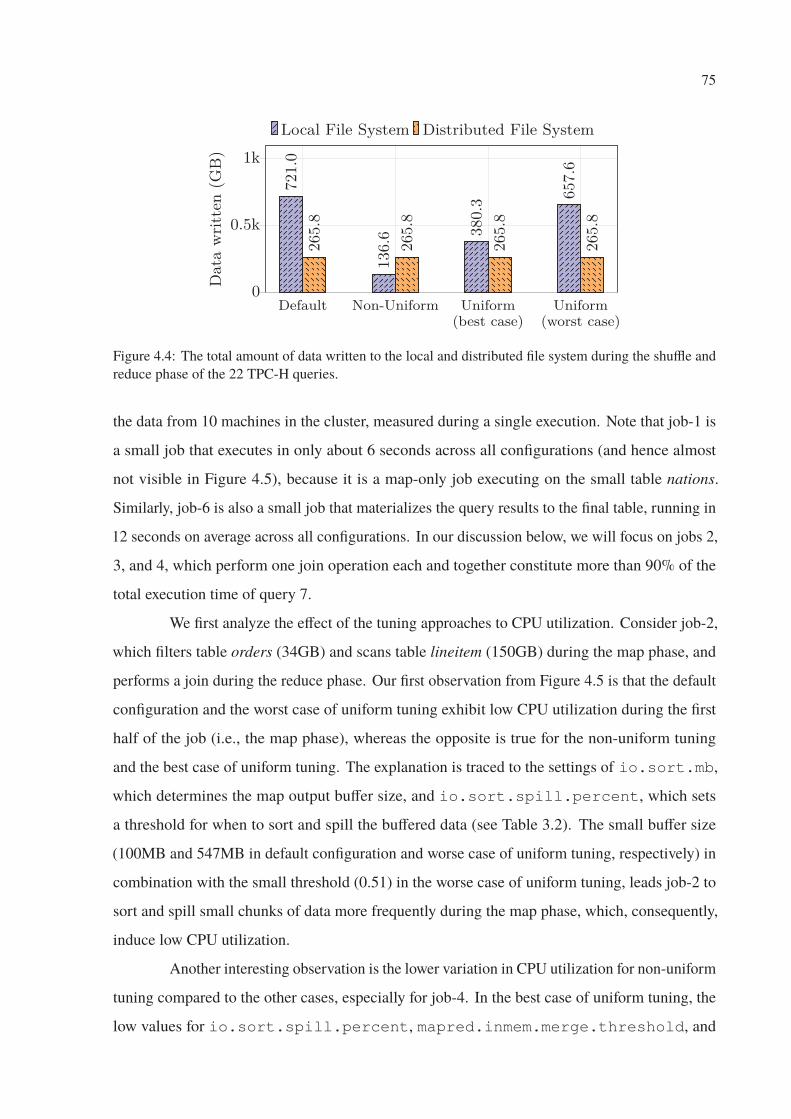
75

721.

0

136.

6 380.

3 657.

6

265.

8

265.

8

265.

8

265.

8

Figure 4.4: The total amount of data written to the local and distributed file system during the shuffle and

reduce phase of the 22 TPC-H queries.

the data from 10 machines in the cluster, measured during a single execution. Note that job-1 is

a small job that executes in only about 6 seconds across all configurations (and hence almost

not visible in Figure 4.5), because it is a map-only job executing on the small table nations.

Similarly, job-6 is also a small job that materializes the query results to the final table, running in

12 seconds on average across all configurations. In our discussion below, we will focus on jobs 2,

3, and 4, which perform one join operation each and together constitute more than 90% of the

total execution time of query 7.

We first analyze the effect of the tuning approaches to CPU utilization. Consider job-2,

which filters table orders (34GB) and scans table lineitem (150GB) during the map phase, and

performs a join during the reduce phase. Our first observation from Figure 4.5 is that the default

configuration and the worst case of uniform tuning exhibit low CPU utilization during the first

half of the job (i.e., the map phase), whereas the opposite is true for the non-uniform tuning

and the best case of uniform tuning. The explanation is traced to the settings of io.sort.mb,

which determines the map output buffer size, and io.sort.spill.percent, which sets

a threshold for when to sort and spill the buffered data (see Table 3.2). The small buffer size

(100MB and 547MB in default configuration and worse case of uniform tuning, respectively) in

combination with the small threshold (0.51) in the worse case of uniform tuning, leads job-2 to

sort and spill small chunks of data more frequently during the map phase, which, consequently,

induce low CPU utilization.

Another interesting observation is the lower variation in CPU utilization for non-uniform

tuning compared to the other cases, especially for job-4. In the best case of uniform tuning, the

low values for io.sort.spill.percent, mapred.inmem.merge.threshold, and

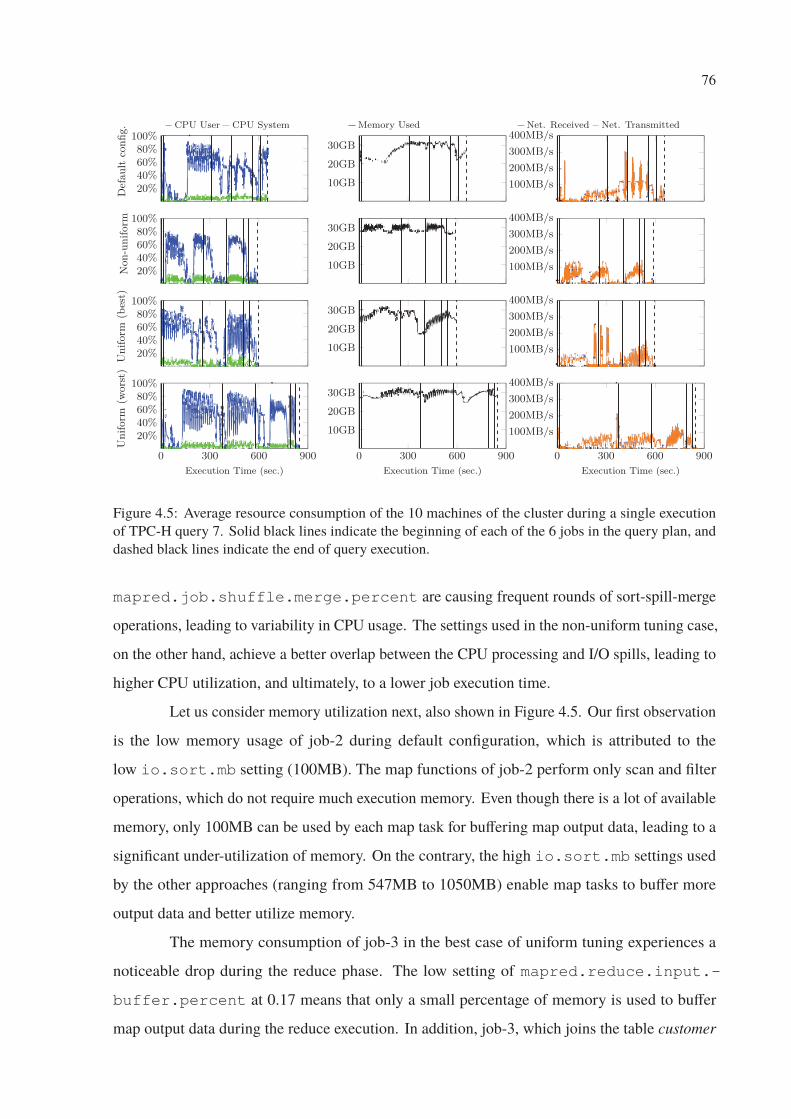
76

0 300 600 900 0 300 600 900 0 300 600 900

Figure 4.5: Average resource consumption of the 10 machines of the cluster during a single execution

of TPC-H query 7. Solid black lines indicate the beginning of each of the 6 jobs in the query plan, and

dashed black lines indicate the end of query execution.

mapred.job.shuffle.merge.percent are causing frequent rounds of sort-spill-merge

operations, leading to variability in CPU usage. The settings used in the non-uniform tuning case,

on the other hand, achieve a better overlap between the CPU processing and I/O spills, leading to

higher CPU utilization, and ultimately, to a lower job execution time.

Let us consider memory utilization next, also shown in Figure 4.5. Our first observation

is the low memory usage of job-2 during default configuration, which is attributed to the

low io.sort.mb setting (100MB). The map functions of job-2 perform only scan and filter

operations, which do not require much execution memory. Even though there is a lot of available

memory, only 100MB can be used by each map task for buffering map output data, leading to a

significant under-utilization of memory. On the contrary, the high io.sort.mb settings used

by the other approaches (ranging from 547MB to 1050MB) enable map tasks to buffer more

output data and better utilize memory.

The memory consumption of job-3 in the best case of uniform tuning experiences a

noticeable drop during the reduce phase. The low setting of mapred.reduce.input.-

buffer.percent at 0.17 means that only a small percentage of memory is used to buffer

map output data during the reduce execution. In addition, job-3, which joins the table customer

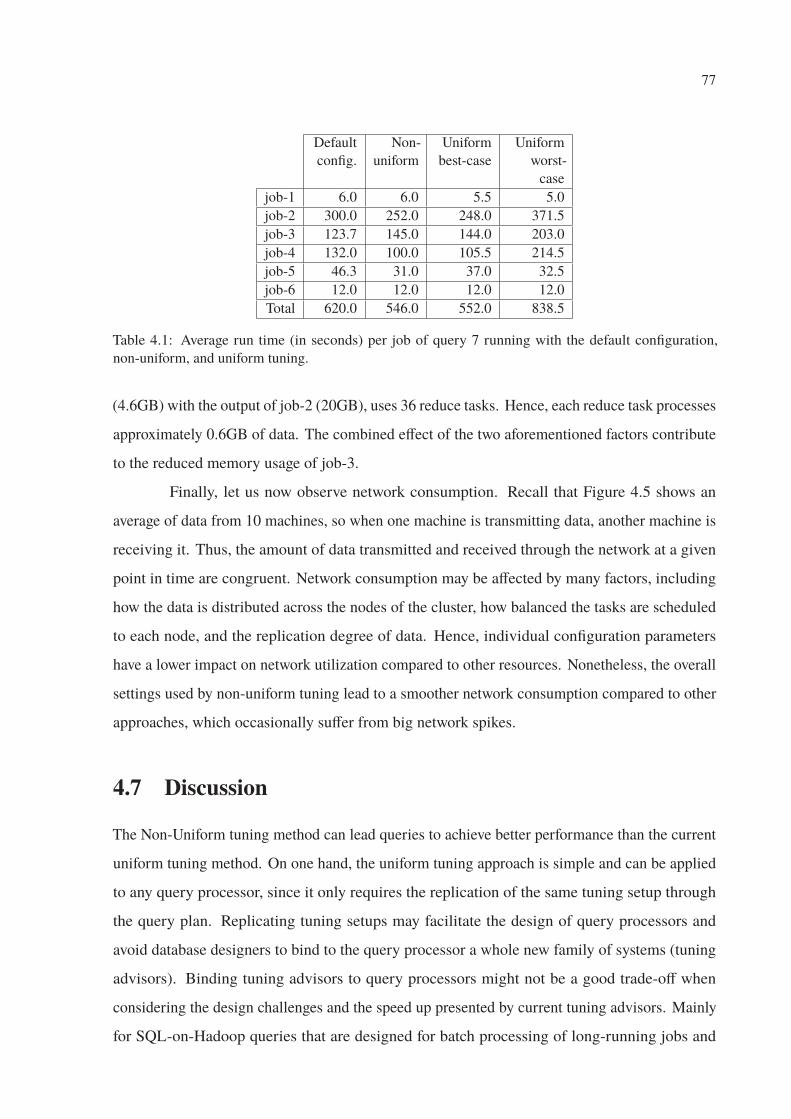
77

Default

config.

Non-

uniform

Uniform

best-case

Uniform

worst-

case

job-1 6.0 6.0 5.5 5.0

job-2 300.0 252.0 248.0 371.5

job-3 123.7 145.0 144.0 203.0

job-4 132.0 100.0 105.5 214.5

job-5 46.3 31.0 37.0 32.5

job-6 12.0 12.0 12.0 12.0

Total 620.0 546.0 552.0 838.5

Table 4.1: Average run time (in seconds) per job of query 7 running with the default configuration,

non-uniform, and uniform tuning.

(4.6GB) with the output of job-2 (20GB), uses 36 reduce tasks. Hence, each reduce task processes

approximately 0.6GB of data. The combined effect of the two aforementioned factors contribute

to the reduced memory usage of job-3.

Finally, let us now observe network consumption. Recall that Figure 4.5 shows an

average of data from 10 machines, so when one machine is transmitting data, another machine is

receiving it. Thus, the amount of data transmitted and received through the network at a given

point in time are congruent. Network consumption may be affected by many factors, including

how the data is distributed across the nodes of the cluster, how balanced the tasks are scheduled

to each node, and the replication degree of data. Hence, individual configuration parameters

have a lower impact on network utilization compared to other resources. Nonetheless, the overall

settings used by non-uniform tuning lead to a smoother network consumption compared to other

approaches, which occasionally suffer from big network spikes.

4.7 Discussion

The Non-Uniform tuning method can lead queries to achieve better performance than the current

uniform tuning method. On one hand, the uniform tuning approach is simple and can be applied

to any query processor, since it only requires the replication of the same tuning setup through

the query plan. Replicating tuning setups may facilitate the design of query processors and

avoid database designers to bind to the query processor a whole new family of systems (tuning

advisors). Binding tuning advisors to query processors might not be a good trade-off when

considering the design challenges and the speed up presented by current tuning advisors. Mainly

for SQL-on-Hadoop queries that are designed for batch processing of long-running jobs and

78

queries are expected to take long running times. However, the benefits that physical-layer tuning

brings to SQL-on-Hadoop queries includes not only speed ups but also a high impact on the

resource consumption, as demonstrated in Section 4.6.

Thus, on the other hand, the non-uniform tuning implies increasing the complexity

of SQL-on-Hadoop query processors when binding a tuning advisor. Despite the increase

in the design complexity, the better control over resources are evident. Such fine-grained

control of resources might increase as the demand for cloud-based processing engines in shared

environments increases as well.

79

Chapter 5

Recycling Tuning Setups

In this Chapter we present the recycling of tuning setups with the Tuning Cache. We have

implemented the Tuning Cache as an extension of the Hive query processor in the form of a Hash

table, where the keys are code-signatures and the values are the tuning setups. The Tuning Cache

leverages tuning setups generated by the Starfish tuning adviser (Herodotou et al., 2011).

At the best of our knowledge, Starfish is the only cost-based tuning adviser publicly

available for MapReduce frameworks. It generates tuning setups base on execution profiles that

are collected in an off-line profiling phase. Profiling is a costly operation that employs dynamic

instrumentation (BTrace) to monitor the invocation of several methods executing in the map and

reduce tasks. For instance, Starfish can capture the arguments of a specific method to determine

the amount of data being processed, or the time taken to process such data. Profiling overhead is

up to 46% when Starfish is profiling 100% of map and reduce tasks. Starfish is able to profile a

sample of tasks at the cost of degrading the quality of tuning being generated (Herodotou and

Babu, 2010; Herodotou et al., 2011; Herodotou and Babu, 2013). Thus, in these experiments, we

run Starfish with sampling turned off to obtain high-quality tuning profiles.

We use Starfish 0.3.01, which ties us to Hadoop 0.20.2 and Hive 0.6.0, unless stated

otherwise. We point out that the Tuning Cache is a generic data structure not restricted to any

particular version of Hive or Hadoop. We evaluate the TPC-H queries provided for Hive2. The

data has been generated with a scale factor of 10. This amounts to 10.46GB of data when stored

on disk.

Our setup is a cluster with three physical machines, where the distributed file system and

job coordinators were isolate on one machine, so that they do not influence the monitoring and

1Starfish is available at https://www.cs.duke.edu/starfish/release.html.

2See https://issues.apache.org/jira/browse/HIVE-600 for the TPC-H queries.

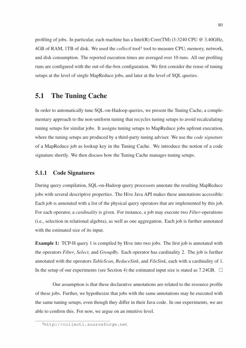
80

profiling of jobs. In particular, each machine has a Intel(R) Core(TM) i3-3240 CPU @ 3.40GHz,

4GB of RAM, 1TB of disk. We used the collectl tool3 tool to measure CPU, memory, network,

and disk consumption. The reported execution times are averaged over 10 runs. All our profiling

runs are configured with the out-of-the-box configuration. We first consider the reuse of tuning

setups at the level of single MapReduce jobs, and later at the level of SQL queries.

5.1 The Tuning Cache

In order to automatically tune SQL-on-Hadoop queries, we present the Tuning Cache, a comple-

mentary approach to the non-uniform tuning that recycles tuning setups to avoid recalculating

tuning setups for similar jobs. It assigns tuning setups to MapReduce jobs upfront execution,

where the tuning setups are produced by a third-party tuning adviser. We use the code signature

of a MapReduce job as lookup key in the Tuning Cache. We introduce the notion of a code

signature shortly. We then discuss how the Tuning Cache manages tuning setups.

5.1.1 Code Signatures

During query compilation, SQL-on-Hadoop query processors annotate the resulting MapReduce

jobs with several descriptive properties. The Hive Java API makes these annotations accessible:

Each job is annotated with a list of the physical query operators that are implemented by this job.

For each operator, a cardinality is given. For instance, a job may execute two Filter-operations

(i.e., selection in relational algebra), as well as one aggregation. Each job is further annotated

with the estimated size of its input.

Example 1: TCP-H query 1 is compiled by Hive into two jobs. The first job is annotated with

the operators Filter, Select, and GroupBy. Each operator has cardinality 2. The job is further

annotated with the operators TableScan, ReduceSink, and FileSink, each with a cardinality of 1.

In the setup of our experiments (see Section 4) the estimated input size is stated as 7.24GB. �

Our assumption is that these declarative annotations are related to the resource profile

of these jobs. Further, we hypothesize that jobs with the same annotations may be executed with

the same tuning setups, even though they differ in their Java code. In our experiments, we are

able to confirm this. For now, we argue on an intuitive level.

3http://collectl.sourceforge.net

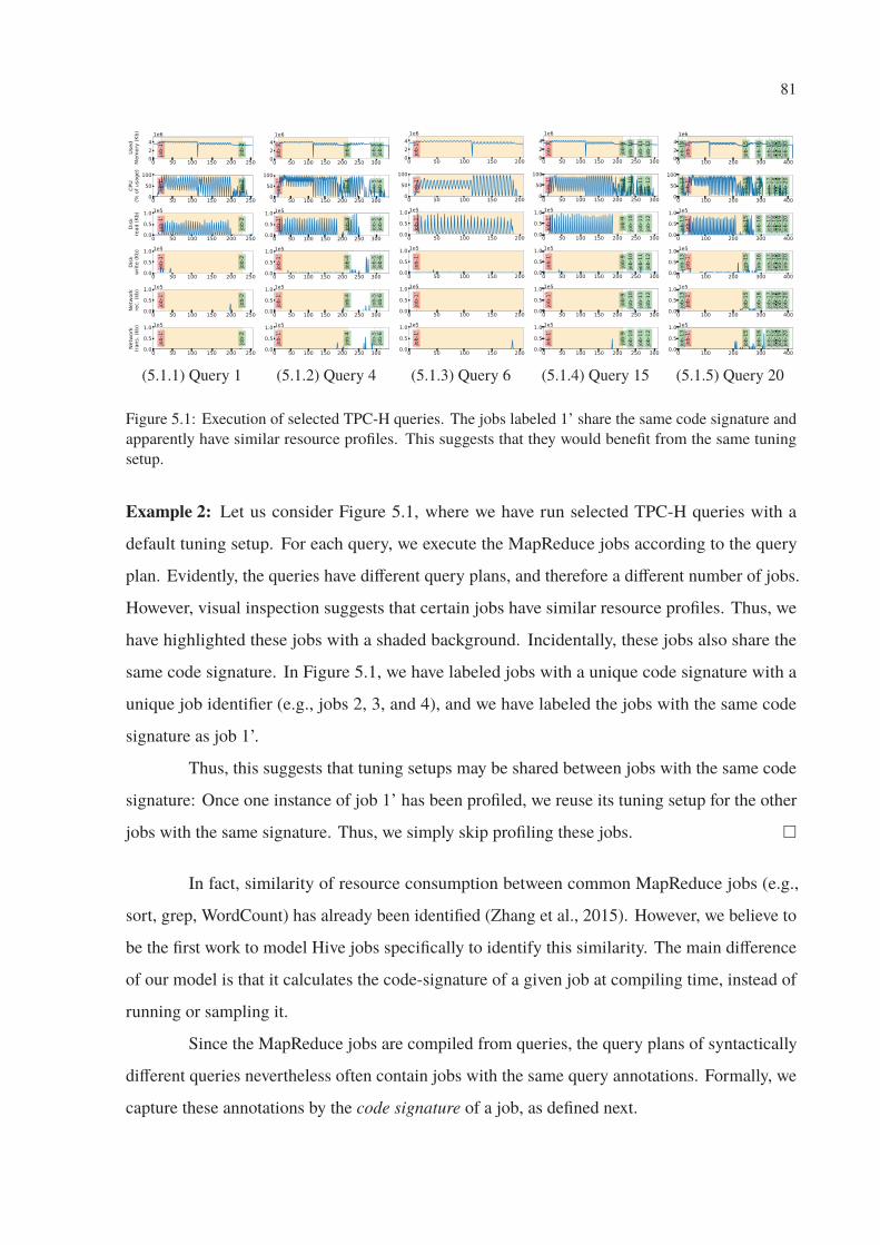
81

(5.1.1) Query 1 (5.1.2) Query 4 (5.1.3) Query 6 (5.1.4) Query 15 (5.1.5) Query 20

Figure 5.1: Execution of selected TPC-H queries. The jobs labeled 1’ share the same code signature and

apparently have similar resource profiles. This suggests that they would benefit from the same tuning

setup.

Example 2: Let us consider Figure 5.1, where we have run selected TPC-H queries with a

default tuning setup. For each query, we execute the MapReduce jobs according to the query

plan. Evidently, the queries have different query plans, and therefore a different number of jobs.

However, visual inspection suggests that certain jobs have similar resource profiles. Thus, we

have highlighted these jobs with a shaded background. Incidentally, these jobs also share the

same code signature. In Figure 5.1, we have labeled jobs with a unique code signature with a

unique job identifier (e.g., jobs 2, 3, and 4), and we have labeled the jobs with the same code

signature as job 1’.

Thus, this suggests that tuning setups may be shared between jobs with the same code

signature: Once one instance of job 1’ has been profiled, we reuse its tuning setup for the other

jobs with the same signature. Thus, we simply skip profiling these jobs. �

In fact, similarity of resource consumption between common MapReduce jobs (e.g.,

sort, grep, WordCount) has already been identified (Zhang et al., 2015). However, we believe to

be the first work to model Hive jobs specifically to identify this similarity. The main difference

of our model is that it calculates the code-signature of a given job at compiling time, instead of

running or sampling it.

Since the MapReduce jobs are compiled from queries, the query plans of syntactically

different queries nevertheless often contain jobs with the same query annotations. Formally, we

capture these annotations by the code signature of a job, as defined next.

82

5.1.2 Code Signature Definition

Consider the query plan definition in Section 3.1, where a job v ∈ V is a tuple of the form

v = (O,D,C) in which Ov is the set of code it executes. Consider that O implements a finite set

of relational algebra operators, thus, O = {o1, . . . , on}, where o is a physical algebra operator.

For instance, Hive version 0.6.0 knows 16 different physical operators.

During query compilation, the query processor assigns the implemented physical query

operators to each job, as well as it annotates several statistics such as their cardinalities. Consider

that we have a function φ : V ×O → N, where V is the set of jobs and O is the set of operators,

and the function φ(v, o) returns the occurrence of each operator o in a job v, that is,

φ(v, o) =

⎧⎨⎩

n job j implements operator o exactly n times

0 otherwise.

Now, consider that we have a function ω : V �→ N, which ω(v) = Δ, where Δ is the

order of magnitude of the expected input data for the given MapReduce job v.

The code signature is the composition of the functions ω and φ. Let us define the code

signature function θ as follows:

Definition 5: The code signature of a MapReduce job v in V is an ordered (|O|+ 1)-tuple,

θ(v) = 〈ω(v), φ(v, o1), φ(v, o2), . . . , φ(v, on)〉 (5.1)

where the first element is always the order of the magnitude of the input data of v, and the

following elements are the occurrence of each operator.

In the following example, we omit operators from the code signature with a cardinality

of zero, for the sake of brevity.

Example 3: We continue with TPC-H query 1. The code signature of the first job is

〈9, Tablescan : 1, Filter : 2, Select : 2, Groupby : 2, Reducesink : 1, Filesink : 1〉

The order of magnitude of the input size is 9.

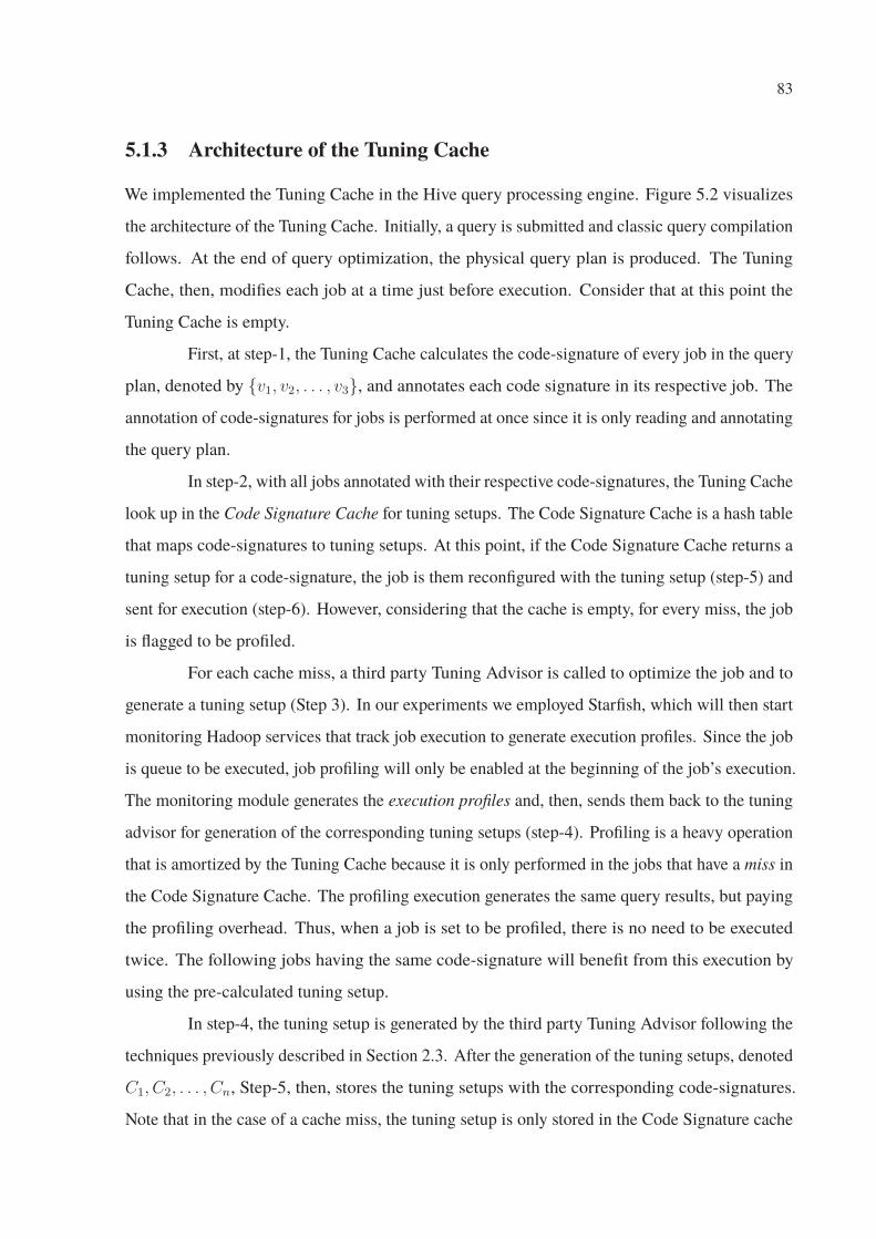
83

5.1.3 Architecture of the Tuning Cache

We implemented the Tuning Cache in the Hive query processing engine. Figure 5.2 visualizes

the architecture of the Tuning Cache. Initially, a query is submitted and classic query compilation

follows. At the end of query optimization, the physical query plan is produced. The Tuning

Cache, then, modifies each job at a time just before execution. Consider that at this point the

Tuning Cache is empty.

First, at step-1, the Tuning Cache calculates the code-signature of every job in the query

plan, denoted by {v1, v2, . . . , v3}, and annotates each code signature in its respective job. The

annotation of code-signatures for jobs is performed at once since it is only reading and annotating

the query plan.

In step-2, with all jobs annotated with their respective code-signatures, the Tuning Cache

look up in the Code Signature Cache for tuning setups. The Code Signature Cache is a hash table

that maps code-signatures to tuning setups. At this point, if the Code Signature Cache returns a

tuning setup for a code-signature, the job is them reconfigured with the tuning setup (step-5) and

sent for execution (step-6). However, considering that the cache is empty, for every miss, the job

is flagged to be profiled.

For each cache miss, a third party Tuning Advisor is called to optimize the job and to

generate a tuning setup (Step 3). In our experiments we employed Starfish, which will then start

monitoring Hadoop services that track job execution to generate execution profiles. Since the job

is queue to be executed, job profiling will only be enabled at the beginning of the job’s execution.

The monitoring module generates the execution profiles and, then, sends them back to the tuning

advisor for generation of the corresponding tuning setups (step-4). Profiling is a heavy operation

that is amortized by the Tuning Cache because it is only performed in the jobs that have a miss in

the Code Signature Cache. The profiling execution generates the same query results, but paying

the profiling overhead. Thus, when a job is set to be profiled, there is no need to be executed

twice. The following jobs having the same code-signature will benefit from this execution by

using the pre-calculated tuning setup.

In step-4, the tuning setup is generated by the third party Tuning Advisor following the

techniques previously described in Section 2.3. After the generation of the tuning setups, denoted

C1, C2, . . . , Cn, Step-5, then, stores the tuning setups with the corresponding code-signatures.

Note that in the case of a cache miss, the tuning setup is only stored in the Code Signature cache

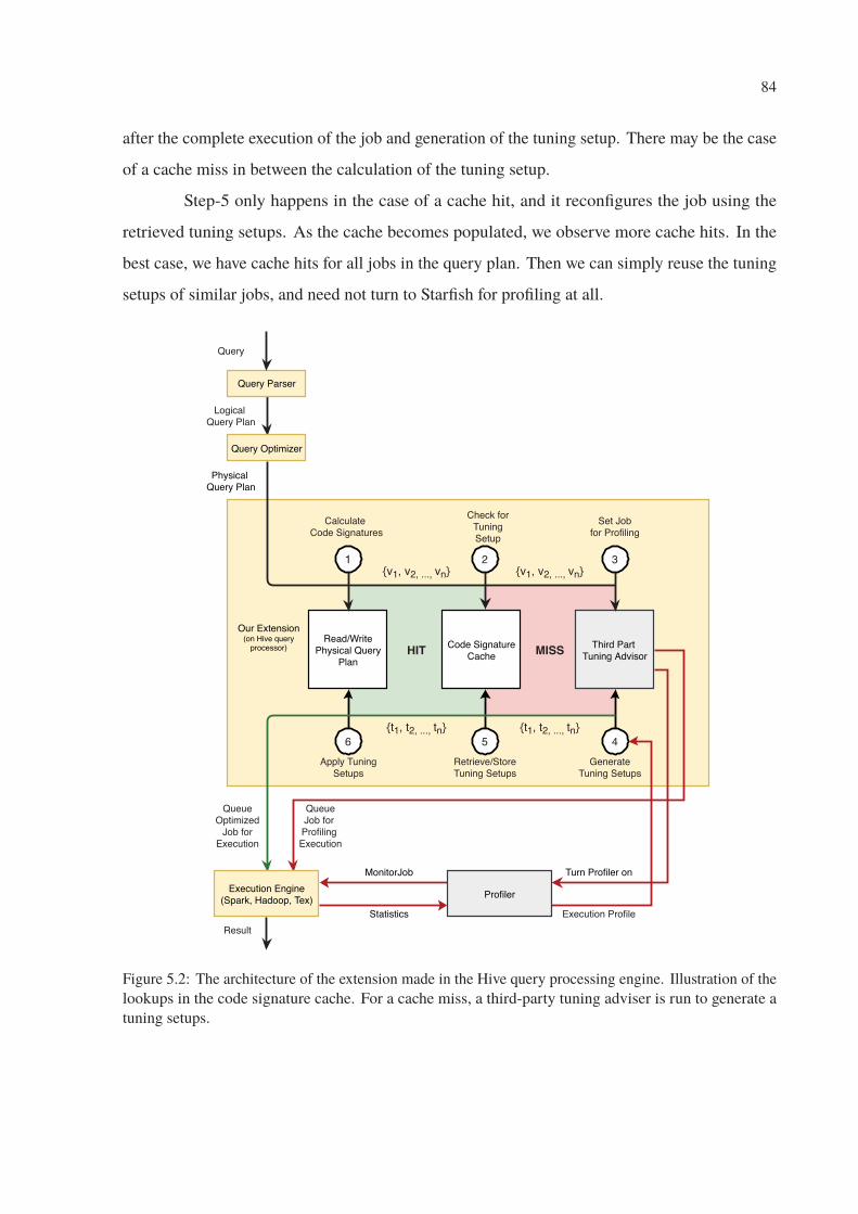
84

after the complete execution of the job and generation of the tuning setup. There may be the case

of a cache miss in between the calculation of the tuning setup.

Step-5 only happens in the case of a cache hit, and it reconfigures the job using the

retrieved tuning setups. As the cache becomes populated, we observe more cache hits. In the

best case, we have cache hits for all jobs in the query plan. Then we can simply reuse the tuning

setups of similar jobs, and need not turn to Starfish for profiling at all.

Read/WritePhysical Query

Plan

Code SignatureCache

Third Part Tuning Advisor

Calculate Code Signatures

QueueOptimized

Job forExecution

6 5 4

321

HIT MISS

{v1, v2, ..., vn} {v1, v2, ..., vn}

{t1, t2, ..., tn} {t1, t2, ..., tn}

Logical Query Plan

Set Jobfor Profiling

Check forTuningSetup

GenerateTuning Setups

Retrieve/StoreTuning Setups

Apply TuningSetups

QueueJob for

ProfilingExecution

Query Parser

Query Optimizer

Physical Query Plan

Execution Engine(Spark, Hadoop, Tex)

Query

Execution Profile

Profiler

MonitorJob

Statistics

Turn Profiler on

Our Extension(on Hive query

processor)

Result

Figure 5.2: The architecture of the extension made in the Hive query processing engine. Illustration of the

lookups in the code signature cache. For a cache miss, a third-party tuning adviser is run to generate a

tuning setups.

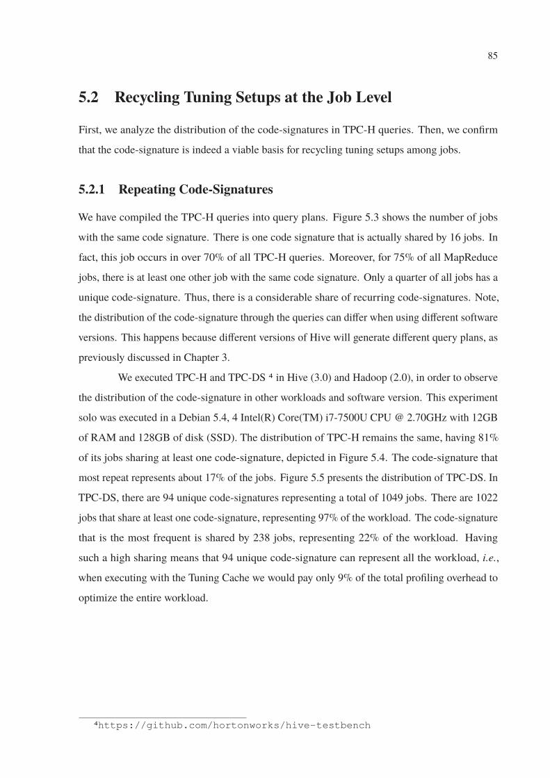
85

5.2 Recycling Tuning Setups at the Job Level

First, we analyze the distribution of the code-signatures in TPC-H queries. Then, we confirm

that the code-signature is indeed a viable basis for recycling tuning setups among jobs.

5.2.1 Repeating Code-Signatures

We have compiled the TPC-H queries into query plans. Figure 5.3 shows the number of jobs

with the same code signature. There is one code signature that is actually shared by 16 jobs. In

fact, this job occurs in over 70% of all TPC-H queries. Moreover, for 75% of all MapReduce

jobs, there is at least one other job with the same code signature. Only a quarter of all jobs has a

unique code-signature. Thus, there is a considerable share of recurring code-signatures. Note,

the distribution of the code-signature through the queries can differ when using different software

versions. This happens because different versions of Hive will generate different query plans, as

previously discussed in Chapter 3.

We executed TPC-H and TPC-DS 4 in Hive (3.0) and Hadoop (2.0), in order to observe

the distribution of the code-signature in other workloads and software version. This experiment

solo was executed in a Debian 5.4, 4 Intel(R) Core(TM) i7-7500U CPU @ 2.70GHz with 12GB

of RAM and 128GB of disk (SSD). The distribution of TPC-H remains the same, having 81%

of its jobs sharing at least one code-signature, depicted in Figure 5.4. The code-signature that

most repeat represents about 17% of the jobs. Figure 5.5 presents the distribution of TPC-DS. In

TPC-DS, there are 94 unique code-signatures representing a total of 1049 jobs. There are 1022

jobs that share at least one code-signature, representing 97% of the workload. The code-signature

that is the most frequent is shared by 238 jobs, representing 22% of the workload. Having

such a high sharing means that 94 unique code-signature can represent all the workload, i.e.,

when executing with the Tuning Cache we would pay only 9% of the total profiling overhead to

optimize the entire workload.

4https://github.com/hortonworks/hive-testbench

86

5 10 15 20 25 30 35 40 45 50

0

5

10

15

20

Distinct Code-Signatures

Num

erof

Jobs

with

this

Code-

Sig

nat

ure

Figure 5.3: MapReduce jobs compiled from TPC-H queries: Counting jobs that share the same code

signature. Executing in Hive 0.6.0 and Hadoop 0.20.0

2 4 6 8 10 12 14 16 18 20 22 24 26 28 30 32 34 36 38

0

5

10

15

20


Num

erof

Jobs

with

this

Code-

Sig

nat

ure

Figure 5.4: MapReduce jobs compiled from TPC-H queries: Counting jobs that share the same code

signature. Executing in Hive 3.0 and Hadoop 2.0.

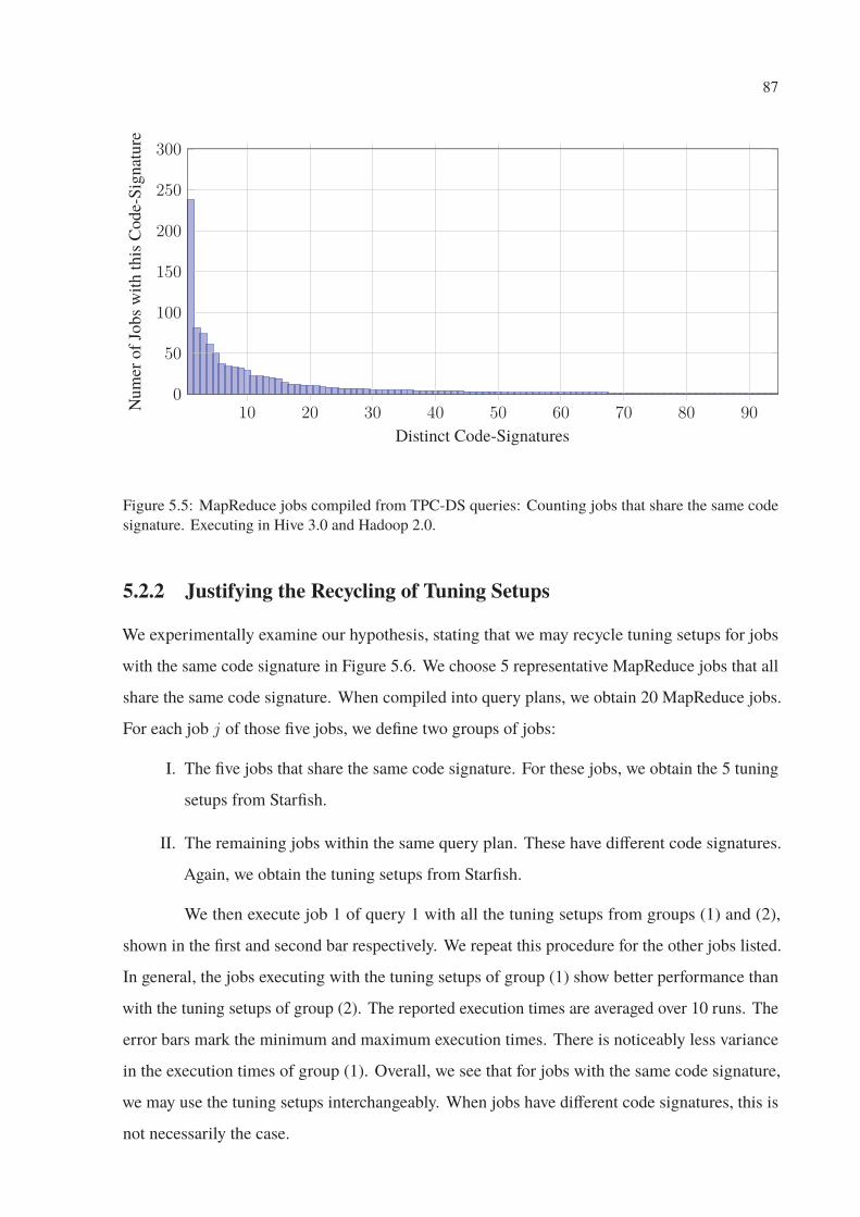
87

10 20 30 40 50 60 70 80 900

50

100

150

200

250

300


Num

erof

Jobs

with

this

Code-

Sig

nat

ure

Figure 5.5: MapReduce jobs compiled from TPC-DS queries: Counting jobs that share the same code

signature. Executing in Hive 3.0 and Hadoop 2.0.

5.2.2 Justifying the Recycling of Tuning Setups

We experimentally examine our hypothesis, stating that we may recycle tuning setups for jobs

with the same code signature in Figure 5.6. We choose 5 representative MapReduce jobs that all

share the same code signature. When compiled into query plans, we obtain 20 MapReduce jobs.

For each job j of those five jobs, we define two groups of jobs:

I. The five jobs that share the same code signature. For these jobs, we obtain the 5 tuning

setups from Starfish.

II. The remaining jobs within the same query plan. These have different code signatures.

Again, we obtain the tuning setups from Starfish.

We then execute job 1 of query 1 with all the tuning setups from groups (1) and (2),

shown in the first and second bar respectively. We repeat this procedure for the other jobs listed.

In general, the jobs executing with the tuning setups of group (1) show better performance than

with the tuning setups of group (2). The reported execution times are averaged over 10 runs. The

error bars mark the minimum and maximum execution times. There is noticeably less variance

in the execution times of group (1). Overall, we see that for jobs with the same code signature,

we may use the tuning setups interchangeably. When jobs have different code signatures, this is

not necessarily the case.

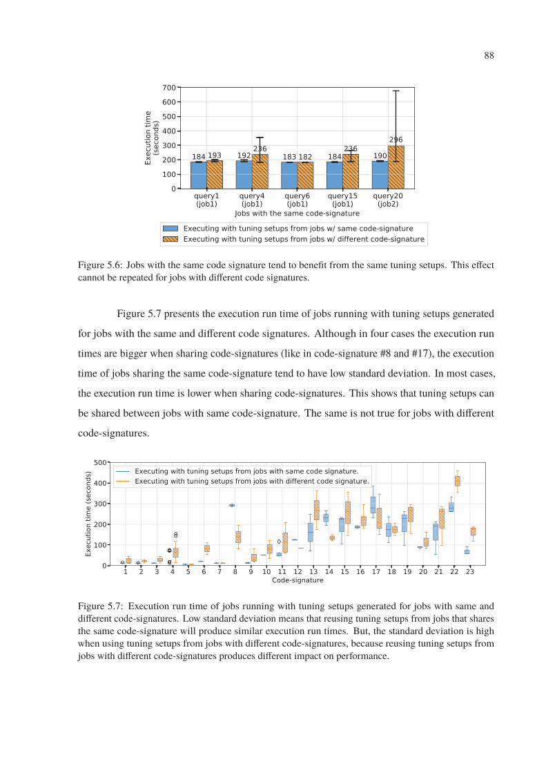
88

Figure 5.6: Jobs with the same code signature tend to benefit from the same tuning setups. This effect

cannot be repeated for jobs with different code signatures.

Figure 5.7 presents the execution run time of jobs running with tuning setups generated

for jobs with the same and different code signatures. Although in four cases the execution run

times are bigger when sharing code-signatures (like in code-signature #8 and #17), the execution

time of jobs sharing the same code-signature tend to have low standard deviation. In most cases,

the execution run time is lower when sharing code-signatures. This shows that tuning setups can

be shared between jobs with same code-signature. The same is not true for jobs with different

code-signatures.

Figure 5.7: Execution run time of jobs running with tuning setups generated for jobs with same and

different code-signatures. Low standard deviation means that reusing tuning setups from jobs that shares

the same code-signature will produce similar execution run times. But, the standard deviation is high

when using tuning setups from jobs with different code-signatures, because reusing tuning setups from

jobs with different code-signatures produces different impact on performance.

89

5.3 Recycling Tuning Setups at the Query Level

We now employ the Tuning Cache for profiling the TPC-H queries. We first profile all 22 queries

in the order specified by the benchmark and discuss the benefits of applying the Tuning Cache.

We then contrast this with the total time spent on profiling if Starfish only samples the JVM

tasks. We also consider different execution orders in profiling the TPC-H queries with the Tuning

Cache, and show that the query order does not have as much impact on profiling time as one

might expect. Finally, we compare the execution time of non-uniform tuning when we have the

Tuning Cache available during profiling and when we profile all jobs with Starfish.

5.3.1 Profiling the TPC-H Queries in Order

We profile the 22 TPC-H queries in the order of the TPC-H benchmark specification. Fig-

ure 5.8(5.8.1) shows the profiling time per query. In total, over ten thousand seconds are spent on

profiling. Even though the runs in Figure 5.8(5.8.1) do not make use the Tuning Cache, for the

purpose of illustration, we visually distinguish two groups of jobs:

I. Jobs which cause a cache miss in the Tuning Cache,

II. and jobs which cause a cache hit in the Tuning cache.

We can observe that for the first TPC-H query, all jobs would cause a cache miss. Yet

already for the second and third queries, we’d have cache hits, even though the savings are minor.

With the Tuning Cache becoming more populated, we get more cache hits, and in some cases,

some substantial savings in the profiling time. For instance, for queries Q6 and Q14, we can

recycle all tuning setups from the cache. Thus, they require no profiling at all.

Let us now turn to the quantitative assessment. In Figure 5.8(5.8.2), we use the Tuning

Cache. Thus, we employ Starfish only for the jobs from group (1), and recycle the tuning setups

for the jobs from group (2). The shaded grey area indicates the height of the original bars from

Figure 5.8(5.8.1), for easier comparison.

Using the Tuning Cache reduces the total time spent on profiling from over ten to below

five thousand seconds. Overall, we can cut down the time spent profiling by more than 50%.

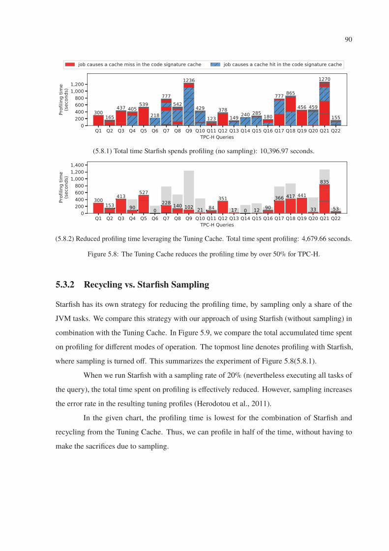
90

(5.8.1) Total time Starfish spends profiling (no sampling): 10,396.97 seconds.

(5.8.2) Reduced profiling time leveraging the Tuning Cache. Total time spent profiling: 4,679.66 seconds.

Figure 5.8: The Tuning Cache reduces the profiling time by over 50% for TPC-H.

5.3.2 Recycling vs. Starfish Sampling

Starfish has its own strategy for reducing the profiling time, by sampling only a share of the

JVM tasks. We compare this strategy with our approach of using Starfish (without sampling) in

combination with the Tuning Cache. In Figure 5.9, we compare the total accumulated time spent

on profiling for different modes of operation. The topmost line denotes profiling with Starfish,

where sampling is turned off. This summarizes the experiment of Figure 5.8(5.8.1).

When we run Starfish with a sampling rate of 20% (nevertheless executing all tasks of

the query), the total time spent on profiling is effectively reduced. However, sampling increases

the error rate in the resulting tuning profiles (Herodotou et al., 2011).

In the given chart, the profiling time is lowest for the combination of Starfish and

recycling from the Tuning Cache. Thus, we can profile in half of the time, without having to

make the sacrifices due to sampling.

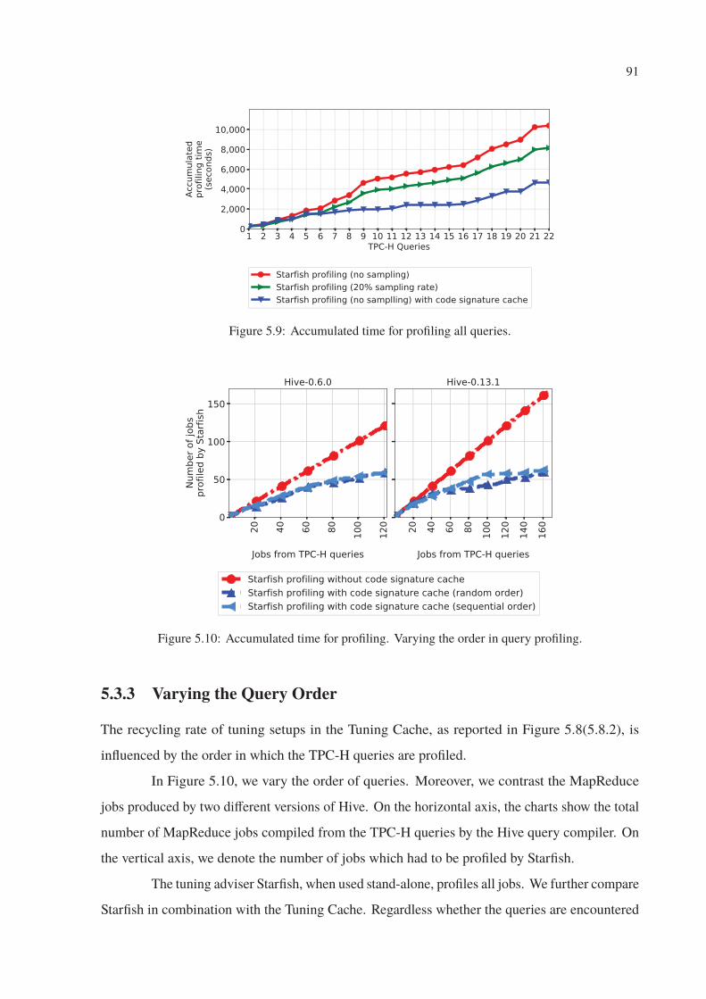
91

Figure 5.9: Accumulated time for profiling all queries.

Figure 5.10: Accumulated time for profiling. Varying the order in query profiling.

5.3.3 Varying the Query Order

The recycling rate of tuning setups in the Tuning Cache, as reported in Figure 5.8(5.8.2), is

influenced by the order in which the TPC-H queries are profiled.

In Figure 5.10, we vary the order of queries. Moreover, we contrast the MapReduce

jobs produced by two different versions of Hive. On the horizontal axis, the charts show the total

number of MapReduce jobs compiled from the TPC-H queries by the Hive query compiler. On

the vertical axis, we denote the number of jobs which had to be profiled by Starfish.

The tuning adviser Starfish, when used stand-alone, profiles all jobs. We further compare

Starfish in combination with the Tuning Cache. Regardless whether the queries are encountered

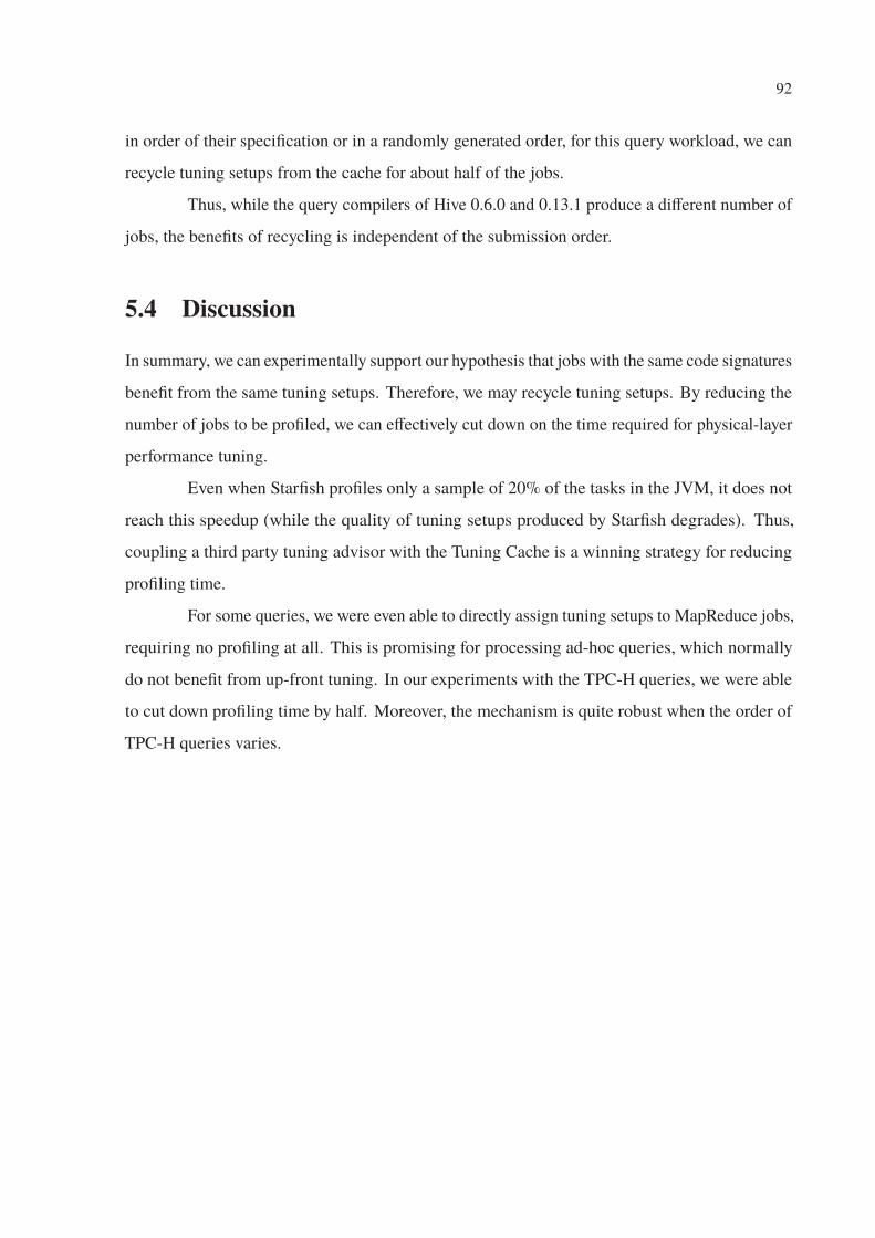
92

in order of their specification or in a randomly generated order, for this query workload, we can

recycle tuning setups from the cache for about half of the jobs.

Thus, while the query compilers of Hive 0.6.0 and 0.13.1 produce a different number of

jobs, the benefits of recycling is independent of the submission order.

5.4 Discussion

In summary, we can experimentally support our hypothesis that jobs with the same code signatures

benefit from the same tuning setups. Therefore, we may recycle tuning setups. By reducing the

number of jobs to be profiled, we can effectively cut down on the time required for physical-layer

performance tuning.

Even when Starfish profiles only a sample of 20% of the tasks in the JVM, it does not

reach this speedup (while the quality of tuning setups produced by Starfish degrades). Thus,

coupling a third party tuning advisor with the Tuning Cache is a winning strategy for reducing

profiling time.

For some queries, we were even able to directly assign tuning setups to MapReduce jobs,

requiring no profiling at all. This is promising for processing ad-hoc queries, which normally

do not benefit from up-front tuning. In our experiments with the TPC-H queries, we were able

to cut down profiling time by half. Moreover, the mechanism is quite robust when the order of

TPC-H queries varies.

93

Chapter 6

Conclusion

6.1 Lessons Learned

While there has been a significant amount of research on automatic parameter tuning for distributed

computing platforms such as Hadoop and Spark (e.g., (Herodotou et al., 2011; Liu et al., 2015;

Shi et al., 2014; Wang et al., 2016; Bao et al., 2018b)), there has been very little work on (i) how

these parameters affect the execution and performance of SQL-on-Hadoop systems, and (ii) how

to tune these parameters within the context of SQL-on-Hadoop workloads. This thesis attempt to

bridge this gap by studying how current Hadoop tuning advisors can be employed for optimizing

the performance of the popular SQL-on-Hadoop engine Hive. The major lessons learned from

our experimental study are:

I. Parameter tuning is important. Tuning the underlying Hadoop parameters can have

a significant impact on both the execution time and the resource utilization of queries

executing on SQL-on-Hadoop systems. In particular, our results reveal that different

parameter settings can cause run time variations between -171% (i.e., 2.8× slower)

and 25% speedup over default settings. At the same time, parameter tuning can have

considerable influence on the resource utilization patterns, leading to better CPU

utilization, improved memory usage, reduced disk usage, and more evenly distributed

network utilization (i.e., fewer spikes).

Reduced resource consumption can have major benefits for both the providers of

Infrastructure-as-a-Service products, as well as their customers. From the customer’s

perspective, non-uniform tuning allows for more efficient resource consumption. De-

pending on the pricing model, lower resource consumption directly translates to lower

94

charges. For instance, storage costs in Amazon AWS Elastic Block Store (EBS) are

$0.10 per GB per month for general purpose (gp2) volumes. The amount of data spilled

to disk for intermediate data, as depicted by Figure 4.4, will be directly reflected in the

billing costs. With reduced data spills, customers could also provision for lower (and

cheaper) I/O per second (IOPS) rates. In addition, lower resource utilization allows

for increased query throughput. Hence, more queries can be executed in the same

amount of time, potentially reducing the cost of cloud deployments. From the provider’s

perspective, the non-uniform tuning has great potential to reduce infrastructure costs,

such as air cooling with more efficient disk usage and data movement, and to increase

machine throughput with less resource consumption and more concurrent clients.

II. Uniform tuning is problematic. The current practice of using one tuning setup per

query (and by extension for all the jobs within each query) suffers from two main

limitations. First, finding a tuning setup that equally benefits all jobs is difficult, if

not impossible, since current Hadoop tuning advisors are designed for tuning one

MapReduce job at-a-time. Hence, even though a particular tuning setup can speed up

one job significantly, it may have a negative effect on other jobs in the same query,

leading to a sub-optimal speedup or even an overall slowdown. Second, the process of

selecting a good tuning setup is time-consuming, as it typically relies on trial-and-error.

Even intuitive strategies such as tuning for the dominant job (i.e., the longest running

job) in a query are not always effective and can actually slow down a query.

III. Non-uniform tuning is promising. Tuning each job in a query independently has been

shown to provide runtime speedups that are similar to the best-observed speedups in our

experiments. In addition, non-uniform tuning is very robust, since the speedup is always

positive, it reduces the need for speculative execution, and, unlike the uniform tuning,

does not suffer from any serious runtime variations. Most importantly, this method

can also lead to considerably better resource utilization for the key resources, namely

CPU, memory, disk, and network. Specifically, both CPU usage and memory paging

were reduced by over 40%, while the total amount of data written to and read from the

local file system was reduced by 5× compared to default settings. The aforementioned

benefits are not bound to Starfish but rather are a consequence of the non-uniform tuning

methodology that optimizes each job independently. We are confident that any Hadoop

95

tuning advisor that can recommend good tuning setups could be used in place of Starfish,

with similar results.

IV. Challenges apply to other SQL-on-Hadoop systems. Even though we focus on

tuning Hadoop parameters for Hive queries, we believe that our experimental results

and conclusions generalize to other SQL-on-Hadoop systems as many of them fork the

source code of Hive, like Shark and Hive on Tez, or present similar query processing

approaches, like SparkSQL, Impala, and Drill. For instance, Impala spans query

fragments to distributed processing deamons that resembles jobs. Impala updates system

health information across all the deamons through a “statestore” component (in Impala

terminology) and keeps all changes in the metadata of the SQL statements in “catalog”

deamons. The non-uniform approach would leverage both deamons to swap tuning

parameters according to the processing needs.

The issues with uniform tuning apply to other types of systems as well. For instance, in

Spark, a job consists of a directed acyclic graph of stages, where each stage comprises a

collection of tasks. Yet, all parameters that affect resource configuration and scheduling

(such as number of cores to use, memory sizes, etc.) are set at the level of jobs and

apply uniformly to all stages and tasks. This problem has already been identified and

efforts are made towards enabling administrators to specify task resource requirements

and configuration at the stage level (SPIP). Currently, Spark tuning advisors such as

(Wang et al., 2016; Singhal and Singh, 2017; Bao et al., 2018b) recommend parameters

at the level of individual jobs. Our findings about the benefits of non-uniform tuning

along with the push towards configuring jobs at the stage level are strong motivators for

building new Spark tuning advisors that fully embrace non-uniform tuning.

V. Recycling Tuning Setups Automated tuning of SQL-on-Hadoop engines and MapRe-

duce frameworks is a highly topical research area. Tuning adviser tools profile

MapReduce jobs to produce suitable tuning setups. Naturally, profiling introduces an

overhead. In pay-as-you-go environments, profiling can drive up the operational costs

considerably. Therefore, ways for reducing the time spent on tuning are of great interest

to the research community and practitioners alike.

Existing tuning advisers cut down the profiling time by sampling, either monitoring only

a share of the JVM tasks (as done by Starfish), by monitoring only a specific sample of

96

MapReduce jobs (as done by PStorM), or running the jobs with a sample of its data set.

Thus, they trade time for the effectiveness of the resulting tuning setup.

Caching tuning setups reduced the profiling time by skipping profiling altogether for

MapReduce jobs where we can recycle the tuning setups from similar jobs. To this end,

we rely on our model of the code signature as a means for identifying similar jobs, and

to populate the Tuning Cache. Our approach is appealingly simple, yet effective, and

lets us cut back on profiling by nearly 50% in case of the TPC-H queries, without major

sacrifices to the quality of tuning setups. Provided that we have successfully profiled

enough similar queries (or rather, their MapReduce jobs), we may even supply ad-hoc

queries with tuning setups, skipping up-front profiling altogether.

VI. Automatic Tuning of SQL-on-Hadoop Systems. In this thesis, we presented that

the performance of SQL-on-Hadoop queries can achieve better performance with

automatic tuning. However, automatic parameter tuning for SQL-on-Hadoop systems

is only possible when combining two approaches: i) the non-uniform tuning method,

presented in Chapter 4, together with ii) the Tuning Cache, a mechanism for recy-

cling tuning setups that enable tuning queries up-front execution. But approaches

were implemented as an extension of Hive query processor, and are enabled with a

hive.optimize.selftuning, completely removing humans from the loop.

With this experimental study, we share our observations with the database research

community. We hope to create an awareness for this problem as well as to initiate new research

on automatic parameter tuning for SQL-on-Hadoop systems.

6.2 Future Work

Most Hadoop tuning advisors (e.g., (Liao et al., 2013; Liu et al., 2015; Ding et al., 2015)),

including Starfish, treat the Map and Reduce functions as black-boxes. However, when the

MapReduce jobs are generated from SQL-on-Hadoop engines, the information regarding the

actual operators comprising the tasks is available. Such information can significantly improve the

performance modeling employed by the tuning advisors, which in turn can improve the tuning

setup recommendations. At the same time, current tuning advisors are designed for optimizing

each job in isolation. However, SQL-on-Hadoop engines typically generate directed acyclic

97

graphs of MapReduce jobs, with various inter-dependencies, as discussed in Section 4.5. Hence,

a new line of tuning advisors that will incorporate query-specific modeling and workflow-aware

tuning is necessary for catering to the specific requirements of SQL-on-Hadoop engines.

As future work, we plan to refine the code signature by integrating the selectivity of

query operators into the code signature. Moreover, we hope to be able to use the Tuning Cache

for application-level tuning as well: By caching power hints for MapReduce jobs, we might be

able to automatically suggest performance hints for similar jobs. This could be a great relief to

the data analyst who has no prior background in database administration.

Another interesting research direction would be to push physical tuning decisions into

the cost optimizer of an SQL-on-Hadoop engine. At optimization time, there is access to

various statistics such as cardinality estimates and possible access paths, which can be used to

(i) improve the effectiveness of the tuning choices, and to (ii) apply the selected tuning choices

to the individual jobs (i.e., in a non-uniform way). The push towards non-uniform tuning also

implies a push towards a fully automated tuning solution. Otherwise, it would be hard, if not

impossible, for an administrator to manually specify parameters for individual jobs that are

generated during a query execution. Overall, as the clusters are growing in size and the workloads

are becoming more complex, it becomes ever more essential for SQL-on-Hadoop systems to

offer self-managing features such as automatic performance tuning.

98

REFERENCES

D. Abadi, A. Ailamaki, D. Andersen, P. Bailis, M. Balazinska, P. Bernstein, P. Boncz, S. Chaudhuri,

A. Cheung, A. Doan, L. Dong, M. J. Franklin, J. Freire, A. Halevy, J. M. Hellerstein,

S. Idreos, D. Kossmann, T. Kraska, S. Krishnamurthy, V. Markl, S. Melnik, T. Milo,

C. Mohan, T. Neumann, B. Chin Ooi, F. Ozcan, J. Patel, A. Pavlo, R. Popa, R. Ramakrishnan,

C. Ré, M. Stonebraker, and D. Suciu. The seattle report on database research. SIGMOD

Rec., 48(4):44–53, Feb. 2020. ISSN 0163-5808. doi: 10.1145/3385658.3385668. URL

https://doi.org/10.1145/3385658.3385668.

F. Afrati, S. Dolev, E. Korach, S. Sharma, and J. D. Ullman. Assignment Problems of Different-

Sized Inputs in MapReduce. ACM Trans. Knowl. Discov. Data, 11(2):18:1–18:35, Dec. 2016.

ISSN 1556-4681. doi: 10.1145/2987376. URL http://doi.acm.org/10.1145/

2987376.

S. Agarwal, B. Mozafari, A. Panda, H. Milner, S. Madden, and I. Stoica. BlinkDB: queries with

bounded errors and bounded response times on very large data. In Proceedings of the 8th ACM

European Conference on Computer Systems - EuroSys ’13, page 29, New York, New York,

USA, apr 2013. ACM Press. ISBN 9781450319942. doi: 10.1145/2465351.2465355. URL

http://dl.acm.org/citation.cfm?id=2465351.2465355.

Apache Software Foundation. Apache Flink. Apache.Org, 2015. URL http://flink.

apache.org/.

M. Armbrust, A. Ghodsi, M. Zaharia, R. S. Xin, C. Lian, Y. Huai, D. Liu, J. K. Bradley, X. Meng,

T. Kaftan, and M. J. Franklin. Spark SQL: Relational Data Processing in Spark. In International

Conference on Management of Data - SIGMOD ’15, pages 1383–1394, New York, New York,

USA, may 2015a. ACM Press. ISBN 9781450327589. doi: 10.1145/2723372.2742797.

99

M. Armbrust, R. S. Xin, C. Lian, Y. Huai, D. Liu, J. K. Bradley, X. Meng, T. Kaftan, M. J. Franklin,

A. Ghodsi, and M. Zaharia. Spark SQL: Relational Data Processing in Spark. In Proceedings

of the 2015 ACM SIGMOD International Conference on Management of Data, SIGMOD ’15,

pages 1383–1394. ACM, 2015b. ISBN 978-1-4503-2758-9. doi: 10.1145/2723372.2742797.

S. Babu. Towards Automatic Optimization of MapReduce Programs. In Proceedings of the

1st ACM Symposium on Cloud Computing, SoCC ’10, pages 137–142. ACM, 2010. ISBN

978-1-4503-0036-0. doi: 10.1145/1807128.1807150.

L. Bao, X. Liu, and W. Chen. Learning-based Automatic Parameter Tuning for Big Data Analytics

Frameworks. In IEEE International Conference on Big Data (Big Data), 2018a.

L. Bao, X. Liu, and W. Chen. Learning-based Automatic Parameter Tuning for Big Data Analytics

Frameworks. In Proc. of the IEEE Intl. Conf. on Big Data, pages 181–190. IEEE, 2018b.

Z. Bei, Z. Yu, H. Zhang, W. Xiong, C. Xu, L. Eeckhout, and S. Feng. RFHOC: A Random-

Forest Approach to Auto-Tuning Hadoop’s Configuration. IEEE Transactions on Parallel and

Distributed Systems, 27(5):1470–1483, May 2016. doi: 10.1109/TPDS.2015.2449299.

Z. Bei, Z. Yu, Q. Liu, C. Xu, S. Feng, and S. Song. MEST: A Model-Driven Efficient

Searching Approach for MapReduce Self-Tuning. IEEE Access, 5:3580–3593, 2017. doi:

10.1109/ACCESS.2017.2672675.

P. A. Boncz, T. Neumann, and O. Erling. Tpc-h analyzed: Hidden messages and lessons learned

from an influential benchmark. In TPCTC, 2013.

P. Bonnet and D. E. Shasha. Physical layer tuning. In Encyclopedia of Database Systems, 2009a.

P. Bonnet and D. E. Shasha. Physical level tuning. In Encyclopedia of Database Systems, 2009b.

P. Bonnet and D. E. Shasha. Application-level tuning. In Encyclopedia of Database Systems,

2009c.

D. Borthakur, S. Rash, R. Schmidt, A. Aiyer, J. Gray, J. S. Sarma, K. Muthukkaruppan,

N. Spiegelberg, H. Kuang, K. Ranganathan, D. Molkov, and A. Menon. Apache hadoop goes

realtime at Facebook. In SIGMOD ’11 - Proceedings of the 2011 international conference

on Management of data, page 1071, New York, New York, USA, jun 2011. ACM Press.

100

ISBN 9781450306614. doi: 10.1145/1989323.1989438. URL http://dl.acm.org/

citation.cfm?id=1989323.1989438.

L. Cai, Y. Qi, and J. Li. A Recommendation-Based Parameter Tuning Approach for Hadoop.

In 2017 IEEE 7th International Symposium on Cloud and Service Computing (SC2), pages

223–230, Nov 2017. doi: 10.1109/SC2.2017.41.

C.-O. Chen, Y.-Q. Zhuo, C.-C. Yeh, C.-M. Lin, and S.-W. Liao. Machine Learning-

Based Configuration Parameter Tuning on Hadoop System. In Proceedings of the 2015

IEEE International Congress on Big Data, BIGDATACONGRESS ’15, pages 386–392,

Washington, DC, USA, 2015. IEEE Computer Society. ISBN 978-1-4673-7278-7. doi:

10.1109/BigDataCongress.2015.64.

Y. Chen, X. Qin, H. Bian, J. Chen, Z. Dong, X. Du, Y. Gao, D. Liu, J. Lu, and H. Zhang. A

Study of SQL-on-Hadoop Systems. In Workshop on Big Data Benchmarks, Performance

Optimization, and Emerging Hardware, pages 154–166, 2014.

L. Cherkasova. Performance Modeling in Mapreduce Environments: Challenges and Oppor-

tunities. In Proceedings of the 2Nd ACM/SPEC International Conference on Performance

Engineering, ICPE ’11, pages 5–6, New York, NY, USA, 2011. ACM. ISBN 978-1-4503-

0519-8. doi: 10.1145/1958746.1958752.

T. Chiba, T. Yoshimura, M. Horie, and H. Horii. Towards Selecting Best Combination of

SQL-on-Hadoop Systems and JVMs. In 11th IEEE International Conference on Cloud

Computing, CLOUD 2018, San Francisco, CA, USA, July 2-7, 2018, pages 245–252, 2018.

doi: 10.1109/CLOUD.2018.00038.

H. E. Ciritoglu, L. B. de Almeida, E. C. de Almeida, T. S. Buda, J. Murphy, and C. Thorpe.

Investigation of replication factor for performance enhancement in the hadoop distributed file

system. In K. Wolter, W. J. Knottenbelt, A. van Hoorn, and M. Nambiar, editors, Companion of

the 2018 ACM/SPEC International Conference on Performance Engineering, ICPE 2018, Berlin,

Germany, April 09-13, 2018, pages 135–140. ACM, 2018. doi: 10.1145/3185768.3186359.

URL https://doi.org/10.1145/3185768.3186359.

J. Dean and S. Ghemawat. MapReduce: Simplified Data Processing on Large Clusters. In OSDI’04,

2004. URL http://dl.acm.org/citation.cfm?id=1251254.1251264.

101

P. M. Deshpande, A. Margoor, and R. Venkatesh. Automatic Tuning of SQL-on-Hadoop Engines

on Cloud Platforms. In 2018 IEEE 11th International Conference on Cloud Computing

(CLOUD), pages 508–515, July 2018. doi: 10.1109/CLOUD.2018.00071.

X. Ding, Y. Liu, and D. Qian. JellyFish: Online Performance Tuning with Adaptive Configuration

and Elastic Container in Hadoop Yarn. In 2015 IEEE 21st International Conference on Parallel

and Distributed Systems (ICPADS), pages 831–836, Dec 2015. doi: 10.1109/ICPADS.2015.112.

X. Ding, Y. Liu, and D. Qian. JellyFish: Online Performance Tuning with Adaptive Configuration

and Elastic Container in Hadoop Yarn. In ICPADS, 2015. ISBN 9780769557854. doi:

10.1109/ICPADS.2015.112.

drill. Drill: Schema-Less Query Execution for Self-Service BI SQL Analytics at Scale, 2019.

https://mapr.com/products/apache-drill/.

M. Ead. PStorM: Profile Storage and Matching for Feedback-Based Tuning of MapReduce

Jobs. In Proceedings of the 17th International Conference on Extending Database Technology,

{EDBT} 2014, Athens, Greece, March 24-28, 2014., 2012.

A. Floratou, U. F. Minhas, and F. Özcan. SQL-on-Hadoop: Full Circle Back to Shared-nothing

Database Architectures. Proc. VLDB Endow., 7(12):1295–1306, Aug. 2014. ISSN 2150-8097.

doi: 10.14778/2732977.2733002.

A. F. Gates, O. Natkovich, S. Chopra, P. Kamath, S. M. Narayanamurthy, C. Olston, R. Benjaminn,

S. Srinavasan, and U. Srivastava. Building a High-Level Dataflow System on top of Map-

Reduce: The Pig Experience. VLDB Endowment, 2009. ISSN 2150-8097. doi: 10.1.1.151.3508.

URL http://www.vldb.org/pvldb/2/vldb09-1074.pdf.

D. Glushkova, P. Jovanovic, and A. Abelló. MapReduce Performance Model for Hadoop 2.x. Inf.

Syst., 79:32–43, 2019.

A. Gounaris. A Methodology for Spark Parameter Tuning. Big Data Research, 2018.

J. Gu, Y. Li, H. Tang, and Z. Wu. Auto-Tuning Spark Configurations Based on Neural Network.

In IEEE International Conference on Communications, 2018.

H. Herodotou and S. Babu. Xplus: a SQL-tuning-aware query optimizer. VLDB Endowment, 3

(1-2):1149–1160, sep 2010. ISSN 2150-8097.

102

H. Herodotou and S. Babu. Profiling, What-if Analysis, and Cost-based Optimization of

MapReduce Programs. Proceedings of the VLDB Endowment, 4(11):1111–1122, 2011.

H. Herodotou and S. Babu. A What-if Engine for Cost-based MapReduce Optimization. IEEE

Data Eng. Bull., 36(1):5–14, 2013.

H. Herodotou, H. Lim, G. Luo, N. Borisov, L. Dong, F. B. Cetin, and S. Babu. Starfish: A

Self-tuning System for Big Data Analytics. CIDR. Vol. 11., 2011.

H. Herodotou, Y. Chen, and J. Lu. A Survey on Automatic Parameter Tuning for Big Data

Processing Systems. ACM Computing Surveys, 53(2):1–37, 2020. ISSN 0360-0300. doi:

10.1145/3381027.

N. Heudecker and M. Adrian. Survey Analysis: Hadoop Adoption Drivers and Challenges.

Gartner, Inc., 2015.

Y. Huai, A. Chauhan, A. Gates, G. Hagleitner, E. N. Hanson, O. O’Malley, J. Pandey, Y. Yuan,

R. Lee, and X. Zhang. Major Technical Advancements in Apache Hive. In Proceedings

of the 2014 ACM SIGMOD International Conference on Management of Data, SIGMOD

’14, pages 1235–1246, New York, NY, USA, 2014. ACM. ISBN 978-1-4503-2376-5. doi:

10.1145/2588555.2595630.

M. Isard, M. Budiu, Y. Yu, A. Birrell, and D. Fetterly. Dryad: distributed data-parallel programs

from sequential building blocks. In SIGOPS/EuroSys European Conference on Computer

Systems, 2007.

A. Jain. Analyzing & optimizing Hadoop performance. In 2017 International Conference on Big

Data Analytics and Computational Intelligence (ICBDAC), pages 116–121, March 2017. doi:

10.1109/ICBDACI.2017.8070820.

D. Jiang, B. C. Ooi, L. Shi, and S. Wu. The Performance of MapReduce: An In-depth Study.

Proceedings of the VLDB Endowment, 3(1-2):472–483, 2010.

T. Johnston, M. Alsulmi, P. Cicotti, and M. Taufer. Performance tuning of MapReduce jobs using

surrogate-based modeling. In Procedia Computer Science, 2015.

A. Katsifodimos and S. Schelter. Apache Flink: Stream Analytics at Scale. IEEE International

Conference on Cloud Engineering Workshop (IC2EW), 2016.

103

A. Khaleel. Optimization of Computing and Networking Resources of a Hadoop Cluster Based

on Software Defined Network. IEEE Access, 2018.

M. Khan, Z. Huang, M. Li, G. A. Taylor, and M. Khan. Optimizing Hadoop parameter settings with

gene expression programming guided PSO. Concurrency Computation, 2017. ISSN 15320634.

doi: 10.1002/cpe.3786. URL http://doi.wiley.com/10.1002/cpe.3786.

M. Kornacker, A. Behm, V. Bittorf, T. Bobrovytsky, C. Ching, A. Choi, J. Erickson, M. Grund,

D. Hecht, M. Jacobs, et al. Impala: A Modern, Open-Source SQL Engine for Hadoop. In

CIDR, volume 1, page 9, 2015.

S. Kumar, S. Padakandla, L. Chandrashekar, P. Parihar, K. Gopinath, and S. Bhatnagar. Scal-

able Performance Tuning of Hadoop MapReduce: A Noisy Gradient Approach. In IEEE

International Conference on Cloud Computing, CLOUD, 2017.

G. J. Lee and J. A. Fortes. Hadoop performance self-tuning using a fuzzy-prediction approach.

In IEEE International Conference on Autonomic Computing, ICAC 2016, 2016.

R. Lee, T. Luo, Y. Huai, F. Wang, Y. He, and X. Zhang. YSmart: Yet Another SQL-to-MapReduce

Translator. In 2011 31st International Conference on Distributed Computing Systems, pages

25–36. IEEE, 2011.

C. Li, H. Zhuang, K. Lu, M. Sun, J. Zhou, D. Dai, and X. Zhou. An Adaptive Auto-configuration

Tool for Hadoop. In IEEE International Conference on Engineering of Complex Computer

Systems, ICECCS, 2014a.

M. Li, L. Zeng, S. Meng, J. Tan, et al. MRONLINE: MapReduce online performance tuning. In

HPDC, 2014b.

G. Liao, K. Datta, T. L. Willke, V. Kalavri, et al. Gunther: Search-based

auto-tuning of MapReduce. Euro-Par, 2013. doi: 10.1007/978-3-642-40047-6.

URLhttp://link.springer.com/10.1007/978-3-642-40047-6 http://

dl.acm.org/citation.cfm?id=2529818.2529869.

H. Lim, H. Herodotou, and S. Babu. Stubby: A Transformation-based Optimizer for MapReduce

Workflows. PVLDB, 5(11):1196–1207, 2012.

104

C. Liu, D. Zeng, H. Yao, C. Hu, et al. MR-COF: A Genetic MapReduce Configuration

Optimization Framework. In Theoretical Computer Science, 2015. ISBN 9783642131356.

doi: 10.1007/978-3-642-13136-3. URL http://www.springerlink.com/index/

10.1007/978-3-642-13136-3.

J. Liu, N. Ravi, S. Chakradhar, and M. Kandemir. Panacea: towards holistic optimization of

MapReduce applications. In CHO, 2012. ISBN 9781450312066. doi: 10.1145/2259016.

2259022. URL http://dl.acm.org/citation.cfm?id=2259016.2259022.

E. R. Lucas Filho. The Uniform Tuning Problem on SQL-On-Hadoop Query Processing. In

SIGMOD SRC, 2017.

A. Menon. Big Data @ Facebook. In MBDS ’12: Proceedings of the 2012 workshop on

Management of big data systems, page 31, New York, New York, USA, sep 2012. ACM Press.

ISBN 9781450317528. doi: 10.1145/2378356.2378364. URL http://dl.acm.org/

citation.cfm?id=2378356.2378364.

D. Miner and A. Shook. MapReduce Design Patterns: Building Effective Algorithms and

Analytics for Hadoop and Other Systems. O’Reilly Media, Inc., 1st edition, 2012a. ISBN

1449327176.

D. Miner and A. Shook. MapReduce Design Patterns: Building Effective Algorithms and

Analytics for Hadoop and Other Systems. O’Reilly Media, Inc., 1st edition, 2012b. ISBN

1449327176, 9781449327170.

N. Nguyen, M. Maifi Hasan Khan, and K. Wang. Towards Automatic Tuning of Apache Spark

Configuration. In IEEE International Conference on Cloud Computing, CLOUD, 2018.

T. Nykiel, M. Potamias, C. Mishra, G. Kollios, et al. MRShare: Sharing across multiple queries

in MapReduce. PVLDB, 3(1-2):494–505, 2010.

T. B. Perez, W. Chen, R. Ji, L. Liu, and X. Zhou. PETS: Bottleneck-aware spark tuning

with parameter ensembles. In International Conference on Computer Communications and

Networks, ICCCN, 2018.

P. Petridis, A. Gounaris, and J. Torres. Spark parameter tuning via trial-and-error. In Advances

in Intelligent Systems and Computing, 2017.

105

N. Poggi, J. L. Berral, T. Fenech, D. Carrera, J. A. Blakeley, U. F. Minhas, and N. Vujic. The

state of SQL-on-Hadoop in the cloud. In BigData, 2016.

J. Pokorny. NoSQL databases: a step to database scalability in web environment. In Proceedings

of the 13th International Conference on Information Integration and Web-based Applications

and Services - iiWAS ’11, page 278, New York, New York, USA, dec 2011. ACM Press. URL

http://dl.acm.org/citation.cfm?id=2095536.2095583.

S. Prabhu, A. P. Rodrigues, M. S. Prasad, and H. R. Nagesh. Performance enhancement of

Hadoop MapReduce framework for analyzing BigData. In IEEE International Conference on

Electrical, Computer and Communication Technologies, ICECCT 2015, 2015.

presto. Presto: Distributed SQL Query Engine for Big Data, 2019. https://prestodb.

github.io/.

A. Rajaraman and J. D. Ullman. Mining of Massive Datasets. Cambridge University Press, New

York, NY, USA, 2011.

S. Sakr, F. M. Orakzai, I. Abdelaziz, and Z. Khayyat. Large-Scale Graph Processing Using Apache

Giraph. Springer Publishing Company, Incorporated, 1st edition, 2017. ISBN 3319474308.

A. D. Sarma, F. N. Afrati, S. Salihoglu, and J. D. Ullman. Upper and Lower Bounds on the Cost

of a Map-Reduce Computation. PVLDB, 2013.

D. Shasha and P. Bonnet. Database tuning: Principles, experiments, and troubleshooting

techniques (part i). In Proceedings of the 2002 ACM SIGMOD International Conference on

Management of Data, SIGMOD ’02, pages 637–637, New York, NY, USA, 2002. ACM. ISBN

1-58113-497-5. doi: 10.1145/564691.564798. URL http://doi.acm.org/10.1145/

564691.564798.

J. Shi, J. Zou, J. Lu, Z. Cao, S. Li, and C. Wang. MRTuner: A Toolkit to Enable Holistic

Optimization for MapReduce Jobs. PVLDB, 2014.

X. Shi, M. Chen, L. He, X. Xie, L. Lu, H. Jin, Y. Chen, and S. Wu. Mammoth: Gearing Hadoop

Towards Memory-Intensive MapReduce Applications. IEEE Transactions on Parallel and

Distributed Systems, 2015.

106

K. Shvachko, H. Kuang, S. Radia, R. Chansler, et al. The Hadoop Distributed File System. In

MSST, volume 10, pages 1–10, 2010.

R. Singhal and P. Singh. Performance Assurance Model for Applications on SPARK Platform.

In Proceedings of the Technology Conference on Performance Evaluation and Benchmarking

(TPCTC), pages 131–146. Springer, 2017.

G. Song, Z. Meng, F. Huet, F. Magoules, et al. A Hadoop MapReduce Performance Prediction

Method. In HPCC 2013, 2013. URL https://hal.archives-ouvertes.fr/hal-

00918329.

SPIP. SPIP: Support Stage level resource configuration and scheduling.

https://issues.apache.org/jira/browse/SPARK-27495, 2019.

M. Stonebraker. SQL databases v. NoSQL databases. Communications of the ACM, 53(4):10, apr

2010. ISSN 00010782. doi: 10.1145/1721654.1721659. URL https://dl.acm.org/

citation.cfm?id=1721659.

M. Stonebraker, D. Abadi, D. J. DeWitt, S. Madden, E. Paulson, A. Pavlo, and A. Rasin.

MapReduce and parallel DBMSs: friends or foes? Communications of the ACM, 53(1):64–71,

2010. ISSN 00010782. doi: 10.1145/1629175.1629197. URL http://portal.acm.

org/citation.cfm?id=1629197.

tajo. Tajo: A Big Data Warehouse System on Hadoop, 2019. https://tajo.apache.org/.

The Apache Software Foundation. Rumen: A tool to extract job characterization data form.

https://hadoop.apache.org/docs/r1.2.1/rumen.html, 2018. [Online; accessed 18-Oct-2018].

A. Thusoo, J. S. Sarma, N. Jain, Z. Shao, P. Chakka, S. Anthony, H. Liu, P. Wyckoff, and

R. Murthy. Hive: a warehousing solution over a map-reduce framework. VLDB Endowment,

2009.

A. Thusoo, J. S. Sarma, N. Jain, Z. Shao, P. Chakka, N. Zhang, S. Antony, H. Liu, and

R. Murthy. Hive - a petabyte scale data warehouse using hadoop. In 2010 IEEE 26th

International Conference on Data Engineering (ICDE 2010), pages 996–1005, March 2010.

doi: 10.1109/ICDE.2010.5447738.

107

TPC. TPC Benchmark H Standard Specification, 2018. http://www.tpc.org/tpch/

spec/tpch2.18.0.pdf.

A. Vaisman and E. Zimnyi. Data Warehouse Systems: Design and Implementation. Springer

Publishing Company, Incorporated, 1st edition, 2016. ISBN 3662513501.

D. Van Aken, A. Pavlo, G. J. Gordon, and B. Zhang. Automatic Database Management System

Tuning Through Large-scale Machine Learning. In SIGMOD, 2017.

L. Viswanathan, A. Jindal, K. Karanasos Microsoft, and K. Karanasos. Query and resource

optimization: Bridging the gap. In International Conference on Data Engineering, ICDE

2018, 2018.

G. Wang, J. Xu, and B. He. A Novel Method for Tuning Configuration Parameters of Spark based

on Machine Learning. In Proc. of the 18th Intl. Conf. on High Performance Computing and

Communications, pages 586–593. IEEE, 2016.

G. Wang, J. Xu, and B. He. A Novel Method for Tuning Configuration Parameters of Spark

Based on Machine Learning. 18th IEEE International Conference on High Performance

Computing and Communications, 14th IEEE International Conference on Smart City and 2nd

IEEE International Conference on Data Science and Systems, HPCC/SmartCity/DSS 2016,

2017.

K. Wang, X. Lin, and W. Tang. Predator-An experience guided configuration optimizer for

Hadoop MapReduce. In IEEE International Conference on Cloud Computing Technology and

Science - CloudCom 2012, 2012.

K. C. Wee and M. S. M. Zahid. Auto-tuned Hadoop MapReduce for ECG analysis. In IEEE

Student Conference on Research and Development, SCOReD 2015, 2015.

D. Wu and A. Gokhale. A self-tuning system based on application Profiling and Performance

Analysis for optimizing Hadoop MapReduce cluster configuration. In International Conference

on High Performance Computing, HiPC 2013, 2013.

R. S. Xin, J. Rosen, M. Zaharia, M. J. Franklin, S. Shenker, and I. Stoica. Shark: SQL and rich

analytics at scale. In Proceedings of the 2013 ACM SIGMOD International Conference on

Management of data, pages 13–24. ACM, 2013.

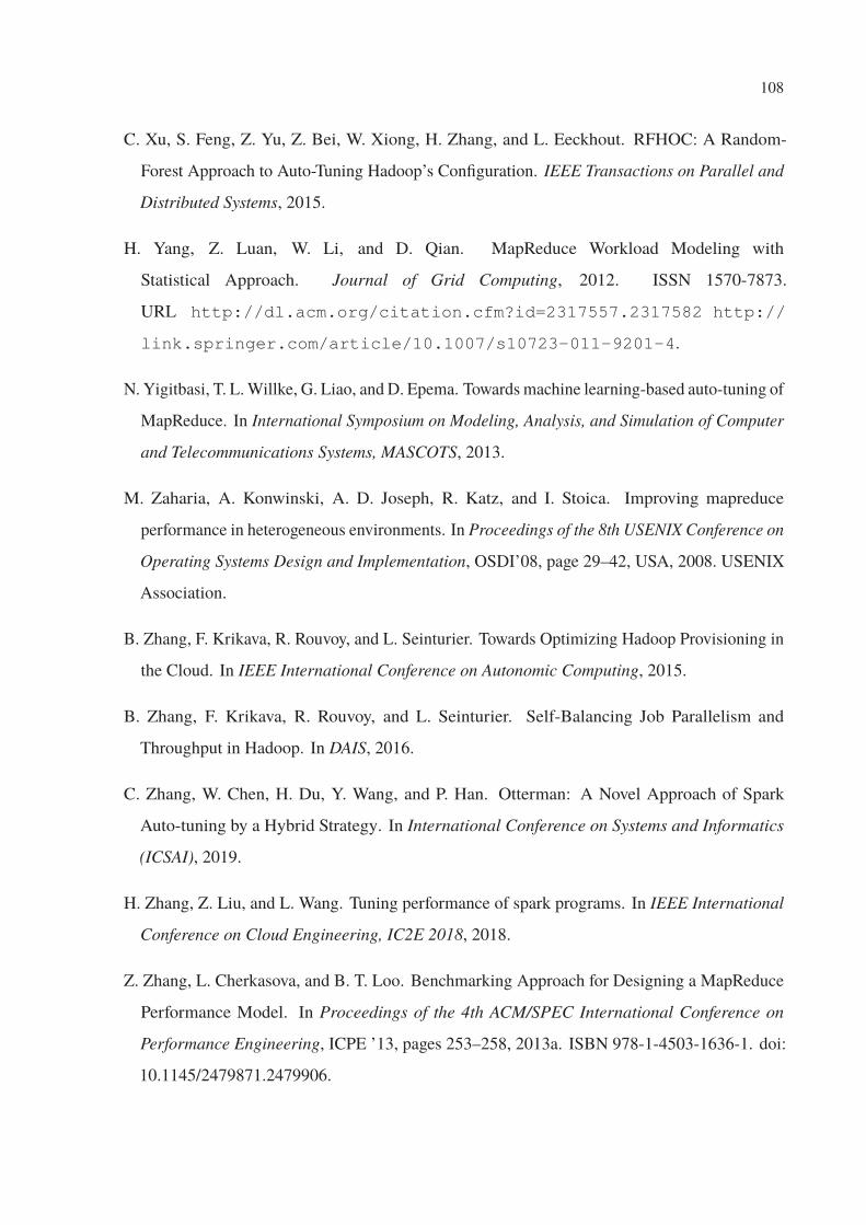
108

C. Xu, S. Feng, Z. Yu, Z. Bei, W. Xiong, H. Zhang, and L. Eeckhout. RFHOC: A Random-

Forest Approach to Auto-Tuning Hadoop’s Configuration. IEEE Transactions on Parallel and

Distributed Systems, 2015.

H. Yang, Z. Luan, W. Li, and D. Qian. MapReduce Workload Modeling with

Statistical Approach. Journal of Grid Computing, 2012. ISSN 1570-7873.

URL http://dl.acm.org/citation.cfm?id=2317557.2317582 http://

link.springer.com/article/10.1007/s10723-011-9201-4.

N. Yigitbasi, T. L. Willke, G. Liao, and D. Epema. Towards machine learning-based auto-tuning of

MapReduce. In International Symposium on Modeling, Analysis, and Simulation of Computer

and Telecommunications Systems, MASCOTS, 2013.

M. Zaharia, A. Konwinski, A. D. Joseph, R. Katz, and I. Stoica. Improving mapreduce

performance in heterogeneous environments. In Proceedings of the 8th USENIX Conference on

Operating Systems Design and Implementation, OSDI’08, page 29–42, USA, 2008. USENIX

Association.

B. Zhang, F. Krikava, R. Rouvoy, and L. Seinturier. Towards Optimizing Hadoop Provisioning in

the Cloud. In IEEE International Conference on Autonomic Computing, 2015.

B. Zhang, F. Krikava, R. Rouvoy, and L. Seinturier. Self-Balancing Job Parallelism and

Throughput in Hadoop. In DAIS, 2016.

C. Zhang, W. Chen, H. Du, Y. Wang, and P. Han. Otterman: A Novel Approach of Spark

Auto-tuning by a Hybrid Strategy. In International Conference on Systems and Informatics

(ICSAI), 2019.

H. Zhang, Z. Liu, and L. Wang. Tuning performance of spark programs. In IEEE International

Conference on Cloud Engineering, IC2E 2018, 2018.

Z. Zhang, L. Cherkasova, and B. T. Loo. Benchmarking Approach for Designing a MapReduce

Performance Model. In Proceedings of the 4th ACM/SPEC International Conference on

Performance Engineering, ICPE ’13, pages 253–258, 2013a. ISBN 978-1-4503-1636-1. doi:

10.1145/2479871.2479906.

109

Z. Zhang, L. Cherkasova, and B. T. Loo. AutoTune: Optimizing Execution Concurrency and

Resource Usage in MapReduce Workflows. In 10th International Conference on Autonomic

Computing, ICAC’13, San Jose, CA, USA, June 26-28, 2013, pages 175–181, 2013b.

110

APPENDIX A – RESOURCE

CONSUMPTION OF TPC-H QUERIES

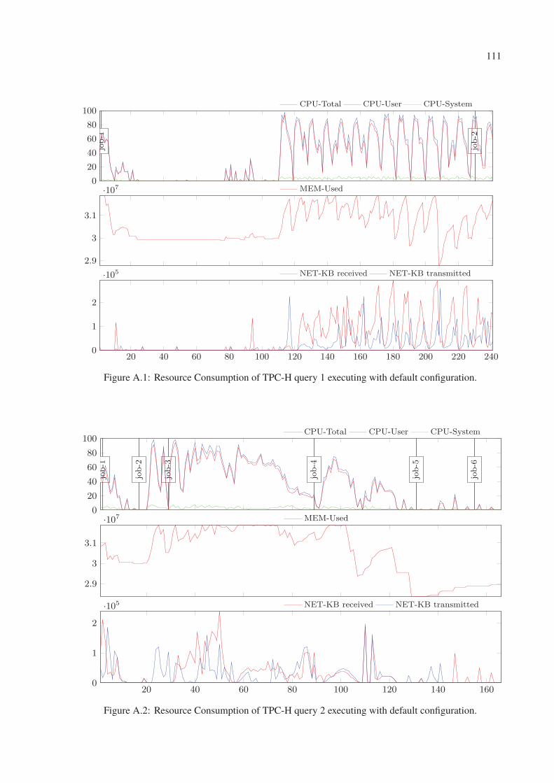
111

0

20

40

60

80

100job-1

job-2

CPU-Total CPU-User CPU-System

2.9

3

3.1

·107 MEM-Used

20 40 60 80 100 120 140 160 180 200 220 2400

1

2

·105 NET-KB received NET-KB transmitted

Figure A.1: Resource Consumption of TPC-H query 1 executing with default configuration.

0

20

40

60

80

100

job-1

job-2

job-3

job-4

job-5

job-6


2.9

3

3.1

·107 MEM-Used

20 40 60 80 100 120 140 1600

1

2



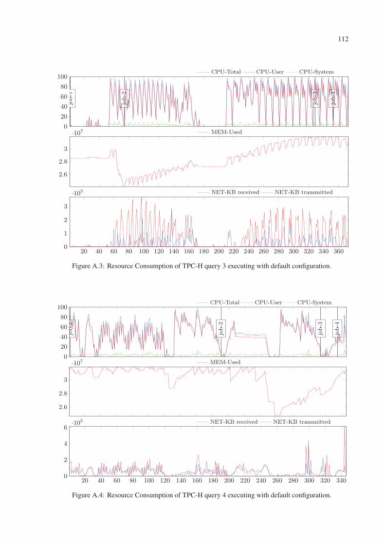
112

0

20

40

60

80

100job-1

job-2

job-3

job-4


2.6

2.8

3

·107 MEM-Used

20 40 60 80 100 120 140 160 180 200 220 240 260 280 300 320 340 3600

1

2

3



0

20

40

60

80

100

job-1

job-2

job-3

job-4


2.6

2.8

3

·107 MEM-Used

20 40 60 80 100 120 140 160 180 200 220 240 260 280 300 320 3400

2

4

6·105 NET-KB received NET-KB transmitted


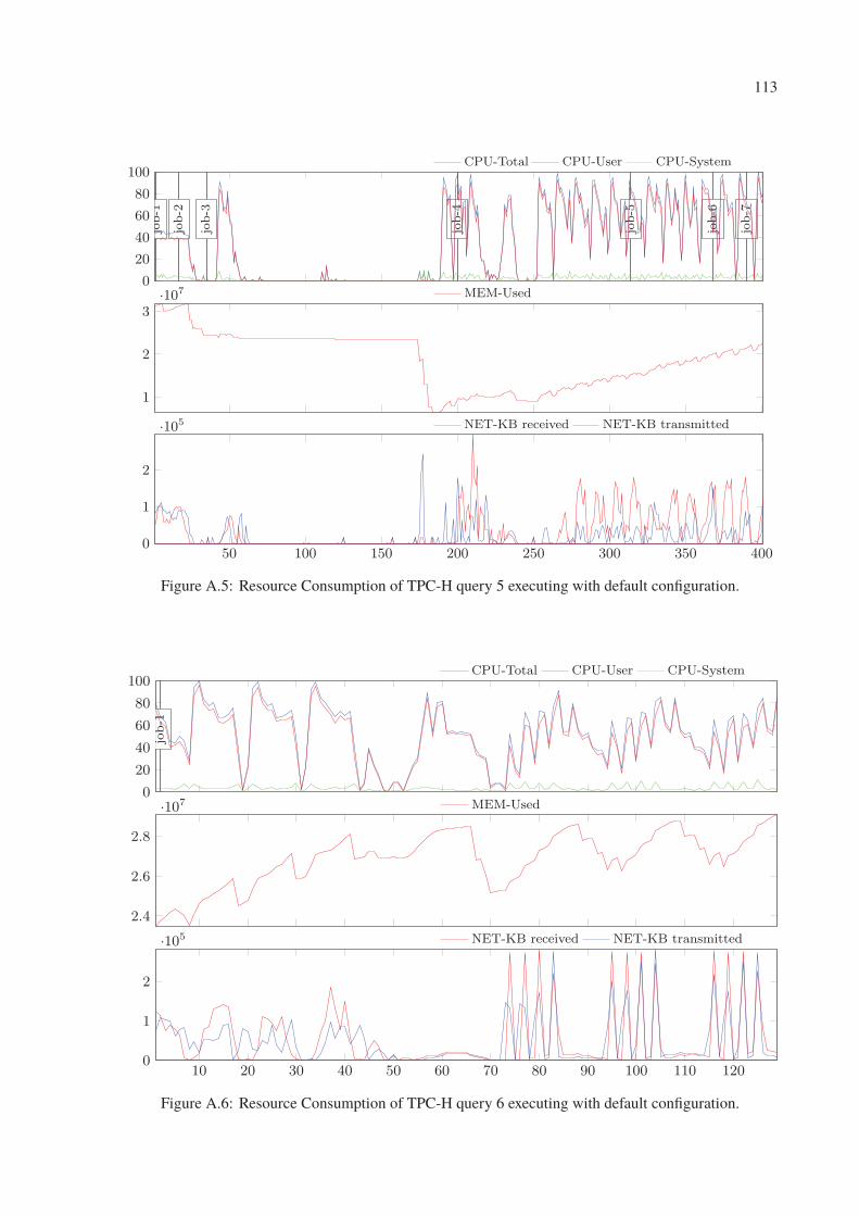
113

0

20

40

60

80

100

job-1

job-2

job-3

job-4

job-5

job-6

job-7


1

2

3·107 MEM-Used

50 100 150 200 250 300 350 4000

1

2



0

20

40

60

80

100

job-1


2.4

2.6

2.8

·107 MEM-Used

10 20 30 40 50 60 70 80 90 100 110 1200

1

2



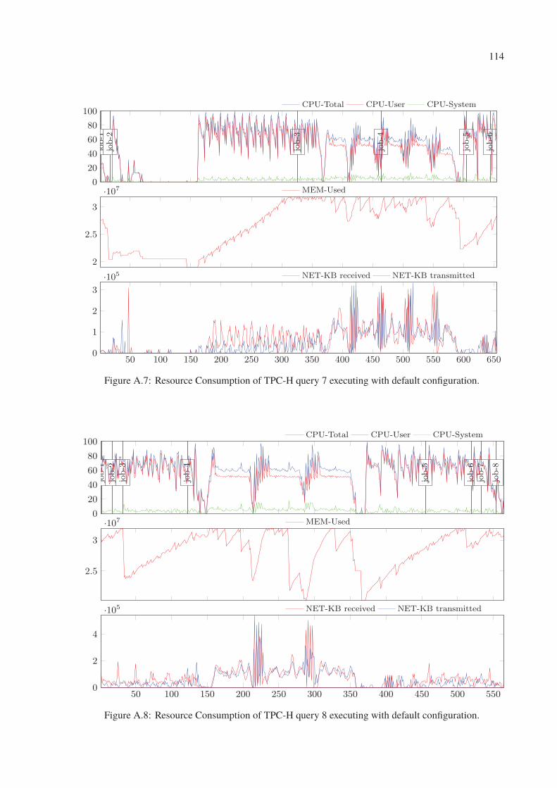
114

0

20

40

60

80

100

job-1

job-2

job-3

job-4

job-5

job-6


2

2.5

3

·107 MEM-Used

50 100 150 200 250 300 350 400 450 500 550 600 6500

1

2

3



0

20

40

60

80

100

job-1

job-2

job-3

job-4

job-5

job-6

job-7

job-8


2.5

3

·107 MEM-Used

50 100 150 200 250 300 350 400 450 500 5500

2

4



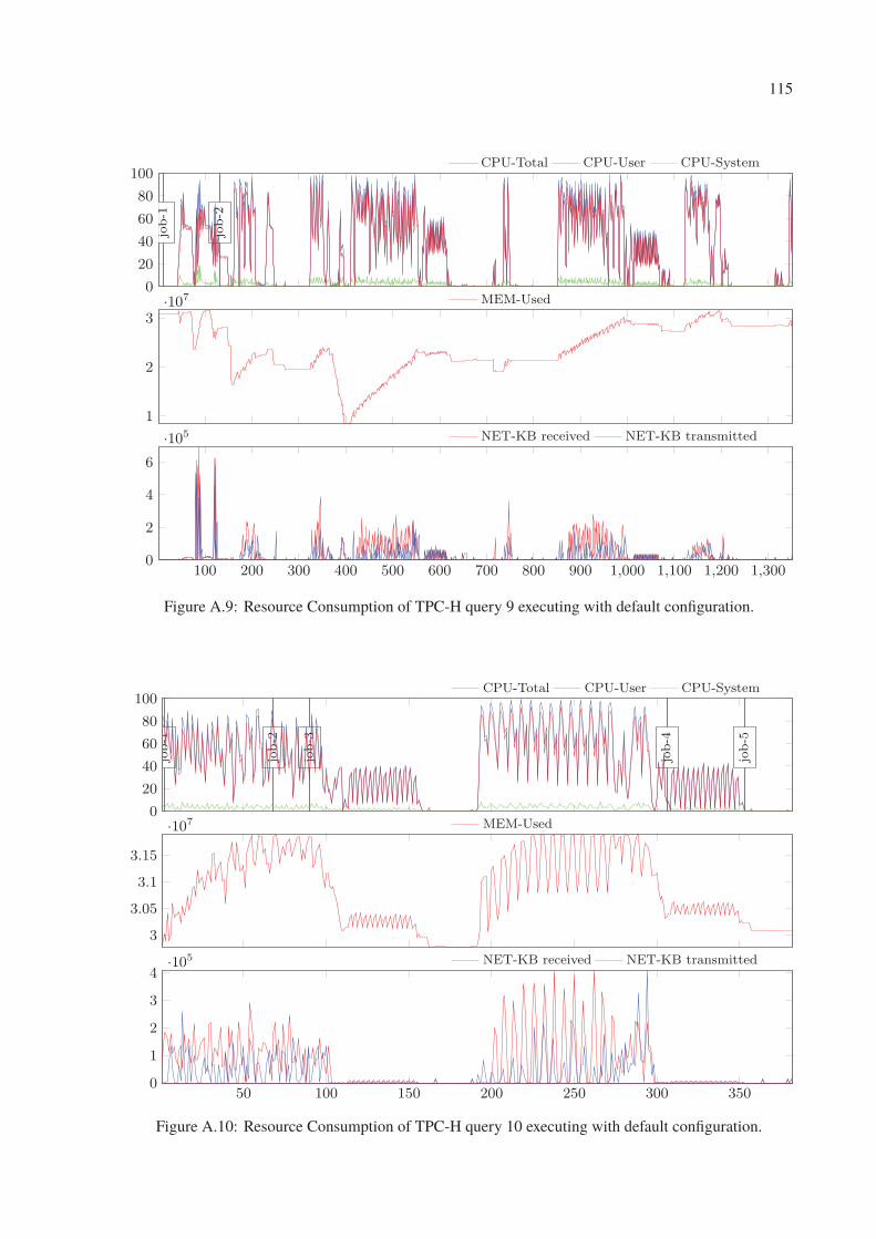
115

0

20

40

60

80

100job-1

job-2


1

2

3·107 MEM-Used

100 200 300 400 500 600 700 800 900 1,000 1,100 1,200 1,3000

2

4

6



0

20

40

60

80

100

job-1

job-2

job-3

job-4

job-5


3

3.05

3.1

3.15

·107 MEM-Used

50 100 150 200 250 300 3500

1

2

3



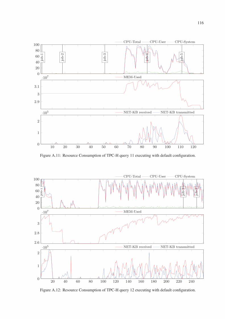
116

0

20

40

60

80

100job-1

job-2

job-3

job-4

job-5


2.9

3

3.1

·107 MEM-Used

10 20 30 40 50 60 70 80 90 100 110 1200

1

2



0

20

40

60

80

100

job-1

job-2

job-3


2.6

2.8

3

·107 MEM-Used

20 40 60 80 100 120 140 160 180 200 220 2400

1

2



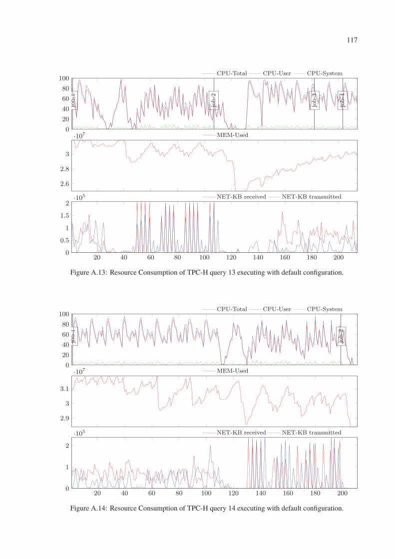
117

0

20

40

60

80

100job-1

job-2

job-3

job-4


2.6

2.8

3

·107 MEM-Used

20 40 60 80 100 120 140 160 180 2000

0.5

1

1.5



0

20

40

60

80

100

job-1

job-2


2.9

3

3.1

·107 MEM-Used

20 40 60 80 100 120 140 160 180 2000

1

2



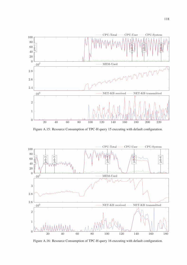
118

0

20

40

60

80

100job-1

job-2

job-3

job-4


2.4

2.6

2.8

·107 MEM-Used

20 40 60 80 100 120 140 160 180 200 2200

1

2



0

20

40

60

80

100

job-1

job-2

job-3

job-4

job-5

job-6


2.6

2.8

3

·107 MEM-Used

20 40 60 80 100 120 140 160 1800

1

2



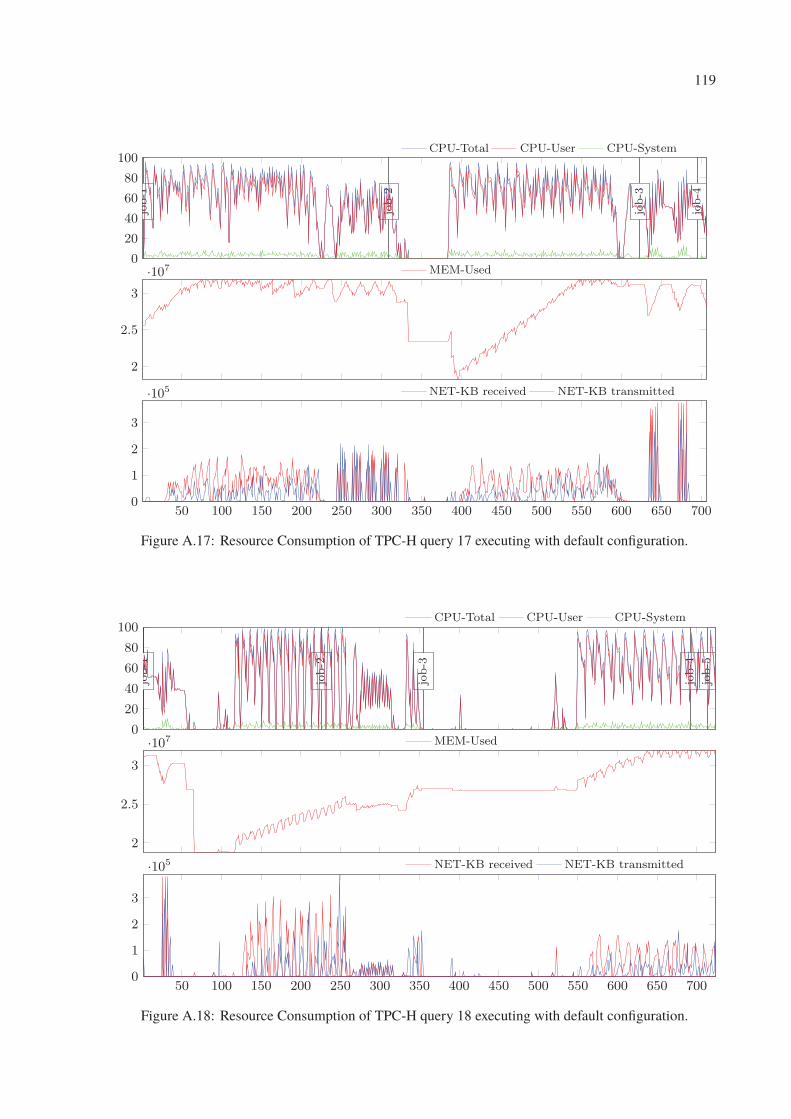
119

0

20

40

60

80

100job-1

job-2

job-3

job-4


2

2.5

3

·107 MEM-Used

50 100 150 200 250 300 350 400 450 500 550 600 650 7000

1

2

3



0

20

40

60

80

100

job-1

job-2

job-3

job-4

job-5


2

2.5

3

·107 MEM-Used

50 100 150 200 250 300 350 400 450 500 550 600 650 7000

1

2

3



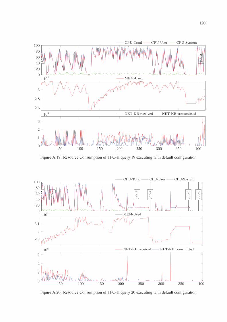
120

0

20

40

60

80

100job-1

job-2


2.6

2.8

3

·107 MEM-Used

50 100 150 200 250 300 350 4000

1

2

3



0

20

40

60

80

100

job-1

job-2

job-3

job-4

job-5

job-6


2.9

3

3.1

·107 MEM-Used

50 100 150 200 250 300 350 4000

2

4



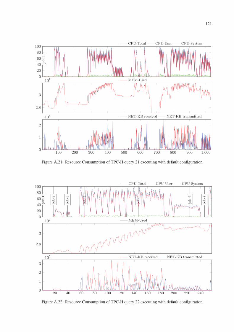
121

0

20

40

60

80

100job-1


2.8

3

·107 MEM-Used

100 200 300 400 500 600 700 800 900 1,0000

1

2



0

20

40

60

80

100

job-1

job-2

job-3

job-4

job-5

job-6

job-7


2.8

3

·107 MEM-Used

20 40 60 80 100 120 140 160 180 200 220 2400

1

2

3



122

APPENDIX B – OCCURRENCE OF

OPERATORS IN TPC-H QUERIES

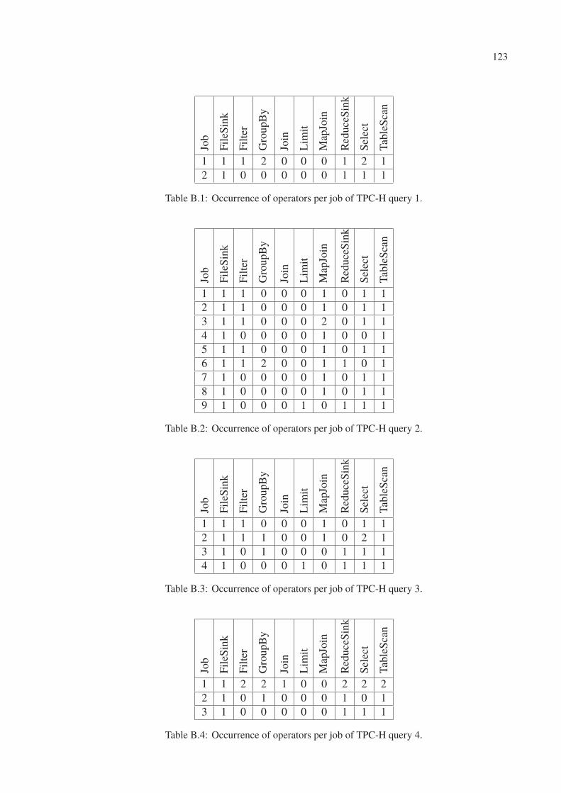
123

Job

FileS

ink

Filte

r

Gro

upB

y

Join

Lim

it

Map

Join

Red

uce

Sin

k

Sel

ect

Tab

leSca

n

1 1 1 2 0 0 0 1 2 1

2 1 0 0 0 0 0 1 1 1

Table B.1: Occurrence of operators per job of TPC-H query 1.Jo

b

FileS

ink

Filte

r

Gro

upB

y

Join

Lim

it

Map

Join

Red

uce

Sin

k

Sel

ect

Tab

leSca

n

1 1 1 0 0 0 1 0 1 1

2 1 1 0 0 0 1 0 1 1

3 1 1 0 0 0 2 0 1 1

4 1 0 0 0 0 1 0 0 1

5 1 1 0 0 0 1 0 1 1

6 1 1 2 0 0 1 1 0 1

7 1 0 0 0 0 1 0 1 1

8 1 0 0 0 0 1 0 1 1

9 1 0 0 0 1 0 1 1 1

Table B.2: Occurrence of operators per job of TPC-H query 2.

Job

FileS

ink

Filte

r

Gro

upB

y

Join

Lim

it

Map

Join

Red

uce

Sin

k

Sel

ect

Tab

leSca

n

1 1 1 0 0 0 1 0 1 1

2 1 1 1 0 0 1 0 2 1

3 1 0 1 0 0 0 1 1 1

4 1 0 0 0 1 0 1 1 1


Job

FileS

ink

Filte

r

Gro

upB

y

Join

Lim

it

Map

Join

Red

uce

Sin

k

Sel

ect

Tab

leSca

n

1 1 2 2 1 0 0 2 2 2

2 1 0 1 0 0 0 1 0 1

3 1 0 0 0 0 0 1 1 1


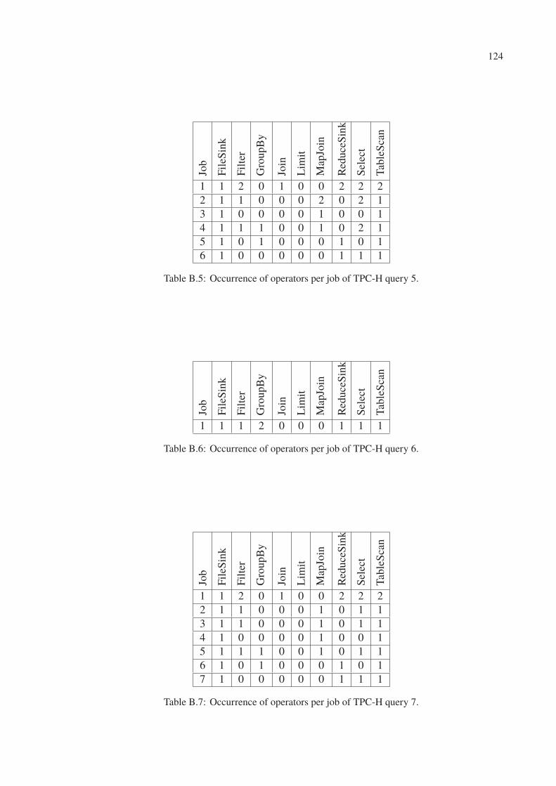
124

Job

FileS

ink

Filte

r

Gro

upB

y

Join

Lim

it

Map

Join

Red

uce

Sin

k

Sel

ect

Tab

leSca

n

1 1 2 0 1 0 0 2 2 2

2 1 1 0 0 0 2 0 2 1

3 1 0 0 0 0 1 0 0 1

4 1 1 1 0 0 1 0 2 1

5 1 0 1 0 0 0 1 0 1

6 1 0 0 0 0 0 1 1 1


Job

FileS

ink

Filte

r

Gro

upB

y

Join

Lim

it

Map

Join

Red

uce

Sin

k

Sel

ect

Tab

leSca

n

1 1 1 2 0 0 0 1 1 1


Job

FileS

ink

Filte

r

Gro

upB

y

Join

Lim

it

Map

Join

Red

uce

Sin

k

Sel

ect

Tab

leSca

n

1 1 2 0 1 0 0 2 2 2

2 1 1 0 0 0 1 0 1 1

3 1 1 0 0 0 1 0 1 1

4 1 0 0 0 0 1 0 0 1

5 1 1 1 0 0 1 0 1 1

6 1 0 1 0 0 0 1 0 1

7 1 0 0 0 0 0 1 1 1


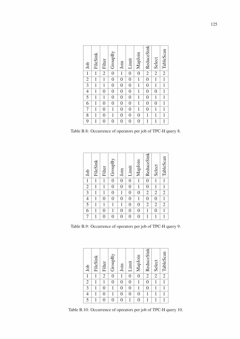
125

Job

FileS

ink

Filte

r

Gro

upB

y

Join

Lim

it

Map

Join

Red

uce

Sin

k

Sel

ect

Tab

leSca

n

1 1 2 0 1 0 0 2 2 2

2 1 1 0 0 0 1 0 1 1

3 1 1 0 0 0 1 0 1 1

4 1 0 0 0 0 1 0 0 1

5 1 1 0 0 0 1 0 1 1

6 1 0 0 0 0 1 0 0 1

7 1 0 1 0 0 1 0 1 1

8 1 0 1 0 0 0 1 1 1

9 1 0 0 0 0 0 1 1 1


Job

FileS

ink

Filte

r

Gro

upB

y

Join

Lim

it

Map

Join

Red

uce

Sin

k

Sel

ect

Tab

leSca

n

1 1 1 0 0 0 1 0 1 1

2 1 1 0 0 0 1 0 1 1

3 1 1 0 1 0 0 2 2 2

4 1 0 0 0 0 1 0 0 1

5 1 1 1 1 0 0 2 2 2

6 1 0 1 0 0 0 1 0 1

7 1 0 0 0 0 0 1 1 1


Job

FileS

ink

Filte

r

Gro

upB

y

Join

Lim

it

Map

Join

Red

uce

Sin

k

Sel

ect

Tab

leSca

n

1 1 2 0 1 0 0 2 2 2

2 1 1 0 0 0 1 0 1 1

3 1 0 1 0 0 1 0 1 1

4 1 0 1 0 0 0 1 1 1

5 1 0 0 0 1 0 1 1 1


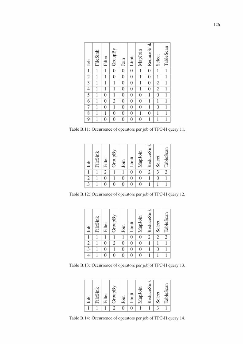
126

Job

FileS

ink

Filte

r

Gro

upB

y

Join

Lim

it

Map

Join

Red

uce

Sin

k

Sel

ect

Tab

leSca

n

1 1 1 0 0 0 1 0 1 1

2 1 1 0 0 0 1 0 1 1

3 1 1 1 0 0 1 0 2 1

4 1 1 1 0 0 1 0 2 1

5 1 0 1 0 0 0 1 0 1

6 1 0 2 0 0 0 1 1 1

7 1 0 1 0 0 0 1 0 1

8 1 1 0 0 0 1 0 1 1

9 1 0 0 0 0 0 1 1 1


Job

FileS

ink

Filte

r

Gro

upB

y

Join

Lim

it

Map

Join

Red

uce

Sin

k

Sel

ect

Tab

leSca

n

1 1 2 1 1 0 0 2 3 2

2 1 0 1 0 0 0 1 0 1

3 1 0 0 0 0 0 1 1 1


Job

FileS

ink

Filte

r

Gro

upB

y

Join

Lim

it

Map

Join

Red

uce

Sin

k

Sel

ect

Tab

leSca

n

1 1 1 1 1 0 0 2 2 2

2 1 0 2 0 0 0 1 1 1

3 1 0 1 0 0 0 1 0 1

4 1 0 0 0 0 0 1 1 1


Job

FileS

ink

Filte

r

Gro

upB

y

Join

Lim

it

Map

Join

Red

uce

Sin

k

Sel

ect

Tab

leSca

n

1 1 1 2 0 0 1 1 3 1


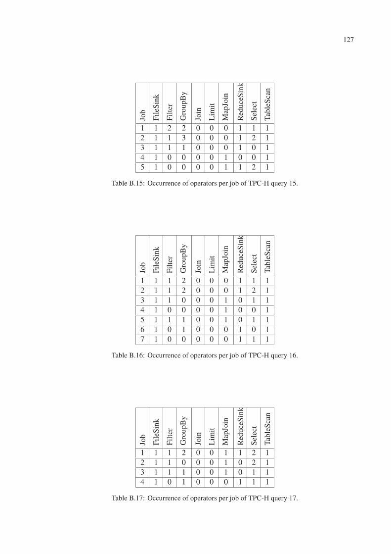
127

Job

FileS

ink

Filte

r

Gro

upB

y

Join

Lim

it

Map

Join

Red

uce

Sin

k

Sel

ect

Tab

leSca

n

1 1 2 2 0 0 0 1 1 1

2 1 1 3 0 0 0 1 2 1

3 1 1 1 0 0 0 1 0 1

4 1 0 0 0 0 1 0 0 1

5 1 0 0 0 0 1 1 2 1


Job

FileS

ink

Filte

r

Gro

upB

y

Join

Lim

it

Map

Join

Red

uce

Sin

k

Sel

ect

Tab

leSca

n

1 1 1 2 0 0 0 1 1 1

2 1 1 2 0 0 0 1 2 1

3 1 1 0 0 0 1 0 1 1

4 1 0 0 0 0 1 0 0 1

5 1 1 1 0 0 1 0 1 1

6 1 0 1 0 0 0 1 0 1

7 1 0 0 0 0 0 1 1 1


Job

FileS

ink

Filte

r

Gro

upB

y

Join

Lim

it

Map

Join

Red

uce

Sin

k

Sel

ect

Tab

leSca

n

1 1 1 2 0 0 1 1 2 1

2 1 1 0 0 0 1 0 2 1

3 1 1 1 0 0 1 0 1 1

4 1 0 1 0 0 0 1 1 1


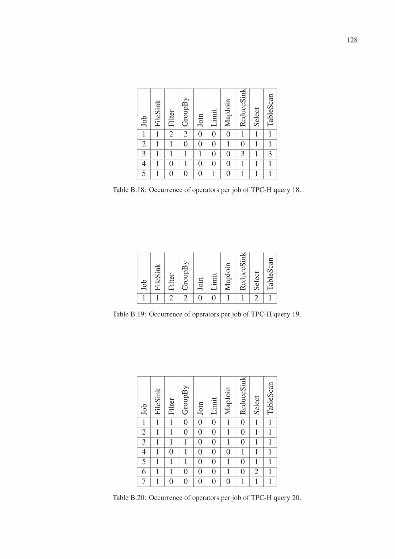
128

Job

FileS

ink

Filte

r

Gro

upB

y

Join

Lim

it

Map

Join

Red

uce

Sin

k

Sel

ect

Tab

leSca

n

1 1 2 2 0 0 0 1 1 1

2 1 1 0 0 0 1 0 1 1

3 1 1 1 1 0 0 3 1 3

4 1 0 1 0 0 0 1 1 1

5 1 0 0 0 1 0 1 1 1


Job

FileS

ink

Filte

r

Gro

upB

y

Join

Lim

it

Map

Join

Red

uce

Sin

k

Sel

ect

Tab

leSca

n

1 1 2 2 0 0 1 1 2 1


Job

FileS

ink

Filte

r

Gro

upB

y

Join

Lim

it

Map

Join

Red

uce

Sin

k

Sel

ect

Tab

leSca

n

1 1 1 0 0 0 1 0 1 1

2 1 1 0 0 0 1 0 1 1

3 1 1 1 0 0 1 0 1 1

4 1 0 1 0 0 0 1 1 1

5 1 1 1 0 0 1 0 1 1

6 1 1 0 0 0 1 0 2 1

7 1 0 0 0 0 0 1 1 1


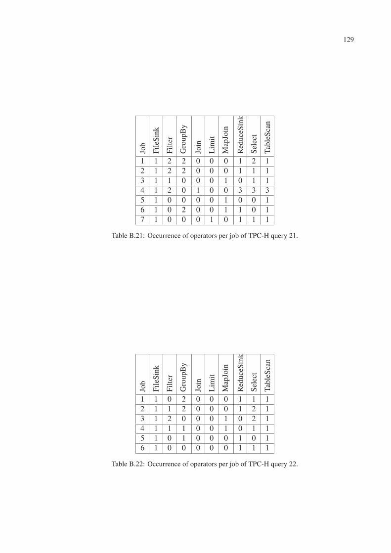
129

Job

FileS

ink

Filte

r

Gro

upB

y

Join

Lim

it

Map

Join

Red

uce

Sin

k

Sel

ect

Tab

leSca

n

1 1 2 2 0 0 0 1 2 1

2 1 2 2 0 0 0 1 1 1

3 1 1 0 0 0 1 0 1 1

4 1 2 0 1 0 0 3 3 3

5 1 0 0 0 0 1 0 0 1

6 1 0 2 0 0 1 1 0 1

7 1 0 0 0 1 0 1 1 1


Job

FileS

ink

Filte

r

Gro

upB

y

Join

Lim

it

Map

Join

Red

uce

Sin

k

Sel

ect

Tab

leSca

n

1 1 0 2 0 0 0 1 1 1

2 1 1 2 0 0 0 1 2 1

3 1 2 0 0 0 1 0 2 1

4 1 1 1 0 0 1 0 1 1

5 1 0 1 0 0 0 1 0 1

6 1 0 0 0 0 0 1 1 1


automatic physical layer tuning of mapreduce …

Documents