brno university of technology - core · brno university of technology vysokÉ uČenÍ technickÉ v...
TRANSCRIPT

BRNO UNIVERSITY OF TECHNOLOGY
VYSOKÉ UČENÍ TECHNICKÉ V BRNĚ
FACULTY OF MECHANICAL ENGINEERING
FAKULTA STROJNÍHO INŽENÝRSTVÍ
INSTITUTE OF SOLID MECHANICS, MECHATRONICS AND BIOMECHANICS
ÚSTAV MECHANIKY TĚLES, MECHATRONIKY A BIOMECHANIKY
A COMPARATIVE STUDY OF ULTIMATE LOAD AND STIFFNESS OF METAL-TO-COMPOSITE JOINTS
SROVNÁVACÍ STUDIE ÚNOSNOSTI A TUHOSTI VYBRANÝCH SPOJŮ KOVOVÉ A KOMPOZITNÍ ČÁSTI KONSTRUKCE
MASTER'S THESIS
DIPLOMOVÁ PRÁCE
AUTHOR
AUTOR PRÁCE
Bc. Michal Tchír
SUPERVISOR
VEDOUCÍ PRÁCE
prof. RNDr. Ing. Jan Vrbka, DrSc., dr. h. c.
BRNO 2016


Abstract
Nowadays, one of the method for joining especially thick and highly loaded composite
components is mechanically fastened bolted joint which allows disassembly of compo-
nents e.g. for repair unlike adhesively bonded joint. Traditional sizing method is first-
ply-failure, however prediction post first-ply-failure behavior is important too. For
structural analysis of the joints as well as for other components is widely used the
finite element method. Since modern nonlinear solvers have capability for investigation
post first-ply-failure behavior of laminate, this capability of one of them was used in
this thesis for investigation of mechanical behavior of laminate made of GFRP layers
which was joined to aluminium bracket using bolts. Progressive damage finite element
models of two metal-to-composite joints were built in order to determine post first-
ply-failure behaviour using three different failure criteria - maximum stress, Hill and
Tsai-Wu using Nastran solver. Force-displacement curves, stiffness-displacement
curves and values of loads at ultimate displacement were compared with experimental
data. As residual stiffness factor influences the results of progressive failure analysis,
sensitivity studies of the factor were done, in which accuracy and achieving conver-
gence were investigated. In the case of the first joint an agreement is less satisfying,
however, the agreement in the case of the second joint, which has a thin steel reinforc-
ing plate on its bottom side, is considerably better. Excellent agreement is especially
with interactive criteria Hill and Tsai-Wu.
Key Words
progressive failure analysis, first ply failure, failure criteria, bolted joints, the finite
element method, composite, laminate, orthotropic material, damage
Abstrakt
V současnosti jedna z metod spojování zejména tlustých a vysoce zatížených
kompozitních komponent je šroubový spoj, který je možné rozebrat pro případ opravy
na rozdíl od lepeného spoje. Kompozitní konstrukce se tradičně dimenzují tak, aby
během provozu nedošlo k porušení první vrstvy laminátu, nicméně důležité je taky
poznat chování laminátu po porušení první vrstvy. Pro strukturální analýzu nejenom
spojů, ale také dalších komponent se používá metoda konečných prvků a protože
moderní nelineání řešiče jsou schopné modelovat chování laminátu po porušení první
vrstvy, tato schopnost jednoho z nich byla využita v této práci při zkoumaní chování
sklolaminátu spojeného s hliníkovou částí šrouby. Konečno-prvkové modely dvou spojů
kovové a kompozitní části konstrukce schopné popsat progresivní porušování laminátu
byly postaveny s využitím tří různých poruchových kritérií – kritéria maximálního
napětí, kritéria Hill a kritéria Tsai-Wu. Problém byl řešen s využitím řešiče Nastran.
Křivky síla-posuv, tuhost-posuv a hodnoty zatížení při hraničním posuvu byly porov-
nány s výsledky experimentů. Jelikož faktor zbytkové tuhosti ovlivňuje výsledky ana-
lýzy progresivního porušování, byly provedeny citlivostní studie zkoumajíci vliv
faktoru na přesnost a stabilitu výpočtu. Shoda výpočtu s experimentem v případe
prvního šroubového spoje je méně uspokojivá, nicméně shoda v případě druhého spoje,
který má zesilující tenkou ocelovou destičku na spodní straně, je podstatně lepší. Vý-
borná shoda je zejména při použití interaktivních kritérií Hill a Tsai-Wu.
Klíčová slova
analýza porušování laminátů, porušení první vrstvy, poruchová kritéria, šroubové
spoje, metóda konečných prvků, kompozit, laminát, ortotropní materiál, poškození

Bibliographic citation
TCHIR, M. A comparative study of ultimate load and stiffness of metal-to-composite
joints. Brno: Brno university of technology, Faculty of mechanical engineering, 2016.
76 pages. Supervisor: prof. RNDr. Ing. Jan Vrbka, DrSc., dr. h. c.
Declaration of originality
I hereby declare that the master’s thesis on the topic A comparative study of ultimate
load and stiffness of metal-to-composite joints I wrote independly using literature and
sources written in the list in the attachment of this thesis.
In Brno 26 May 2016 …………….…………………………..
Acknowledgement
I would like to express gratitude to my supervisor prof. RNDr. Ing. Jan Vrbka, DrSc.,
dr. h. c. for giving me oportunity to work on this interesting topic, his optimism and
useful recommendations, which improved quality of the thesis. I would like to thank
my consultant, Ing. Petr Vosynek, Ph.D., for encouraging me to pursue the topic, for
helpfulness and for professional managing the work on the thesis. I would like to ex-
press my gratitude to M.Sc. Volodymyr Symonov, my consultant at Institute of aero-
space engineering, for introducing me to the world of composite materials, willingness
to answer my questions and a permission to use results of his work in this thesis. I am
grateful to prof. Ing. Přemysl Janíček, DrSc., FEng. for helpful discussion and inspira-
tional advices, which helped to clearify solution of the problem investigated in this
work.
Especially I am grateful to my parents, who have supported me during whole my
studies.
Thank you.
Contents
Introduction ............................................................................................................................. 12
1 Problem situation ............................................................................................................. 13
1.1 Formulation of the problem ..................................................................................... 13
1.2 Objectives of the thesis ............................................................................................. 13
1.3 Type of the problem ................................................................................................. 13
2 System of important quantities ........................................................................................ 15
3 Joints ................................................................................................................................ 16
3.1 Type 1 ....................................................................................................................... 16
3.2 Type 2 ....................................................................................................................... 17
3.3 Failure of bolted joints ............................................................................................. 17
4 Research study ................................................................................................................. 19
5 Mechanics of composite materials .................................................................................... 21
5.1 Constitutive equations for an orthotropic material .................................................. 21
5.2 Failure theories ......................................................................................................... 23
5.2.1 Maximum stress theory ........................................................................................ 23
5.2.2 Energy based interaction theory (Tsai-Hill) ......................................................... 25
5.2.3 Interactive tensor polynomial theory (Tsai-Wu).................................................. 26
5.3 Progressive composite failure .................................................................................... 27
5.4 Strengh ratio ............................................................................................................. 28
6 Solution method ............................................................................................................... 30
6.1 The finite element method ....................................................................................... 30
6.2 Nonlinear solution ..................................................................................................... 32
6.3 Continuum mechanics .............................................................................................. 33
7 Description of computional models and settings of solution............................................ 35
7.1 Geometry .................................................................................................................. 36
7.2 Mesh ......................................................................................................................... 38
7.2.1 Mesh sensitivity study .......................................................................................... 38
7.3 Model of material ..................................................................................................... 39
7.3.1 Sensitivity study of residual stiffness factor ......................................................... 41
7.4 Model of boundary conditions .................................................................................. 42
7.5 Contacts .................................................................................................................... 43
7.6 Model of loads ........................................................................................................... 46
7.7 Setting of the solution ............................................................................................... 48
8 Results .............................................................................................................................. 49
8.1 Type 1 ....................................................................................................................... 50
8.1.1 Comparison of force-displacement curves and stiffness-displacement curves ....... 50
8.1.2 Displacement and failure index using maximum stress failure criterion .............. 51
8.1.3 Displacement and failure index using Hill failure criterion .................................. 52
8.1.4 Displacement and failure index using Tsai-Wu failure criterion* ........................ 53
8.2 Type 2 ....................................................................................................................... 54
8.2.1 Comparison of force-displacement curves and stiffness-displacement curves ....... 54
8.2.2 Displacement and failure index using the maximum stress failure criterion ........ 55
8.2.3 Displacement and failure index using the Hill failure criterion ............................ 56
8.2.4 Displacement and failure index using the Tsai-Wu failure criterion* .................. 57
8.3 Comparison of Type 1 and Type 2 ........................................................................... 58
8.3.1 Evaluation of loads at ultimate displacement ...................................................... 59
9 Discussion ......................................................................................................................... 62
10 Conclusion ........................................................................................................................ 65
List of symbols ......................................................................................................................... 70
List of abreviations and names of software ............................................................................. 72
List of figures ............................................................................................................................ 73
List of tables ............................................................................................................................. 76

11
12
Introduction
Since 1970s the use of fiber composites in aircraft structures has increased and the
main reason is the significant weight-saving and other advantages that these compo-
sites can provide. Nevertheless, the high cost of composites compared with similar
structures made from metal, mainly aluminium alloys, do not allow their use on every
aircraft structural component. Apart from the high cost, composites have long range
of disadvantages, low resistance to mechanical damage, low through-thickness strength
and temperature limitations are only the most important.[7] Engineers need to achieve
the levels of safety given by norms, laws and standards and these days, the finite
element method is widely used for determination stresses and strains in materials,
hence for ensurance the safety in a development phase of a product. Several sizing
methods for composite structures have developed over the last 40 years. One of the
most important method is first-ply failure which is often acceptable to sign off a draw-
ing. However, progressive failure analysis allows to describe the post first-ply-failure
behavior of a structure. Nowadays, engineers use progressive failure analyses for better
understanding of the structure, increasing realiability and saving costs. In this thesis
progressive failure analyses using the finite element method of metal-to-composite
bolted joints are described.
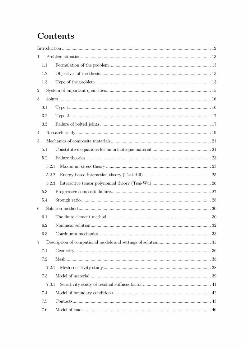
Fig. 1 Airbus A350XWB has fuselage and wings made of CFRP. [32]
13
1 Problem situation
According to Janíček [1]:
„A problem situation is a nonstandard situation unlike a standard situation, because
different activities than routine, known or algorithmizable have to be used for a solu-
tion. “
Since the use of fiber composites in aircraft structures is increasing, therefore a need
of an effective joining exists and one of the method of joining especially thick composite
components is use of bolted joints. Traditional sizing method of composites is first-ply-
failure analysis, but the FPF may lead to very conservative sizing, therefore engineers
and scientists are interested in post first-ply-failure behavior of material these days.
Other reasons can be increasing realiability and safety of structure.
1.1 Formulation of the problem
Investigation of post first-ply-failure behavior of two bolted joints with emphasis on
laminate using three different failure criteria by the finite element method and com-
parison of results from finite element analyses with experimental data.
1.2 Objectives of the thesis
„An objective is a statement formulated by a subject about an intention to do or to
create something, where an impulse for the intention comes from the subject or its
surround. [1]“
The aim of the thesis is computational modelling of post first-ply-failure behavior of
selected metal-to-composite joints with emphasis on laminate. Objectives, which
should be done, are described below:
• to build a computational models of the joints involved geometry models, mate-
rial models with three different failure criteria, model of boundary conditions
and loads,
• to do progressive failure analyses of the joints with respective failure criteria,
• to determine force-displacement curves, stiffness-displacement curves and ulti-
mate loads if possible,
• to compare the results of finite element analyses with experimental data,
• to evaluate the results.
1.3 Type of the problem
Since the problem has technical character, knowledge of mechanics of materials, con-
tinuum mechanics, mathematics and materials is needed – the problem is multidisci-
plinary.
14
In adition, the problem is causal, because the bindings to the enviroment are known
as well as its geometry and activation. The problem is direct because the inputs are
known. However, outputs, that had been measured, are known too, which can help to
asses the results of progressive failure analysis. Geometry, boundary conditions, mate-
rial characteristics are given, and the aim is to determine force-displacement curves,
stiffness-displacement curves, and ultimate load if possible.
According to Janíček [9], an experiment has five utilizations:
reduction experiment
verification experiment
formulational experiment
experiment for concretization
experiment for identification
In this work the experimental data will be used for determination of loads at ultimate
displacement and for verification of results of the progressive failure analyses.
15
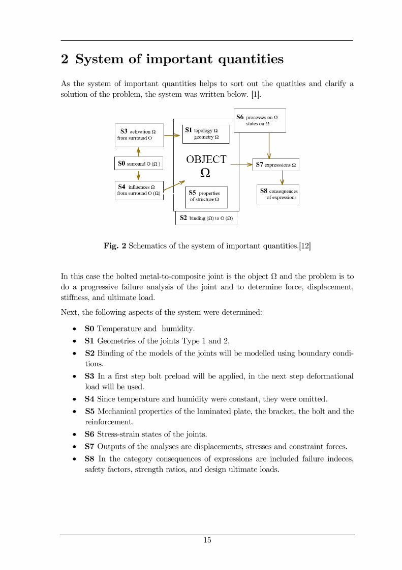
2 System of important quantities
As the system of important quantities helps to sort out the quatities and clarify a
solution of the problem, the system was written below. [1].
Fig. 2 Schematics of the system of important quantities.[12]
In this case the bolted metal-to-composite joint is the object Ω and the problem is to
do a progressive failure analysis of the joint and to determine force, displacement,
stiffness, and ultimate load.
Next, the following aspects of the system were determined:
S0 Temperature and humidity.
S1 Geometries of the joints Type 1 and 2.
S2 Binding of the models of the joints will be modelled using boundary condi-
tions.
S3 In a first step bolt preload will be applied, in the next step deformational
load will be used.
S4 Since temperature and humidity were constant, they were omitted.
S5 Mechanical properties of the laminated plate, the bracket, the bolt and the
reinforcement.
S6 Stress-strain states of the joints.
S7 Outputs of the analyses are displacements, stresses and constraint forces.
S8 In the category consequences of expressions are included failure indeces,
safety factors, strength ratios, and design ultimate loads.
16
3 Joints
Due the facts written in the Introduction, a combination of common materials like
metals and composites is getting more popular and as a result of the combination of
materials, the need of effective joining exists. According to Baker [7], three categories
of joint types are used: mechanically fastened joints using bolts and rivets, adhesively
bonded joints using a polymeric adhesive and a combination of mechanical fastening
and adhesive bonding. Intuitively, it may be concluded that mechanical fastening is
an unsatisfactory means of joining composites because the fastener holes must cut
fibers, destroying part of the load path. However, since considerable loss in strength
occurs (typically to half of the original strength), the only feasible or economic use of
bolted joints is joining highly loaded thick composite components.[7] Nevertheless, ac-
cording to Heimbs, Schmeer, Blaurock and Steeger [18] “The use of carbon fibre-rein-
forced plastic materials for primary aircraft structures is ever expanding in the last
decades with the fuselage of the latest generation of large commercial aircraft, i.e.
Airbus A350XWB and Boeing 787, being built with this composite material. Despite
considerable progress in adhesive bonding technologies, the connection of composite
structural elements is still mainly based on mechanically fastened bolted joints, allowing
for component disassembly e.g. for repair.”
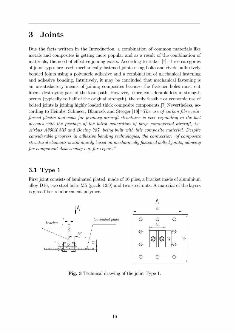
3.1 Type 1
First joint consists of laminated plated, made of 16 plies, a bracket made of aluminium
alloy D16, two steel bolts M5 (grade 12.9) and two steel nuts. A material of the layers
is glass fiber reinforcement polymer.
Fig. 3 Technical drawing of the joint Type 1.
laminated plate bracket

17
3.2 Type 2
Second joint similarly like the joint Type 1 consists of laminated plated, made of 16
plies, a bracket made of aluminium alloy D16, two bolts M5 (grade 12.9), two nuts
and, in adition, a steel reinforcement on the bottom of the plate as shown in Fig. 4.
The material of the layers is same as in the case of Type 1.
Fig. 4 Technical drawing of the joint Type 2.
3.3 Failure of bolted joints
According to Baker [7], main failure modes in mechanical joints in composites in-
clude net-tension failure, cleavage tension, essentially mixed tension/shear; bolt-head
pulling through the laminate, a problem particularly with deeply countersunk holes;
and bolt failure due to bearing failure.
Fig. 5 Schematic illustration of main failure modes in mechanical joints in
composites.[15]
laminated plate bracket
reinforcemeent
18
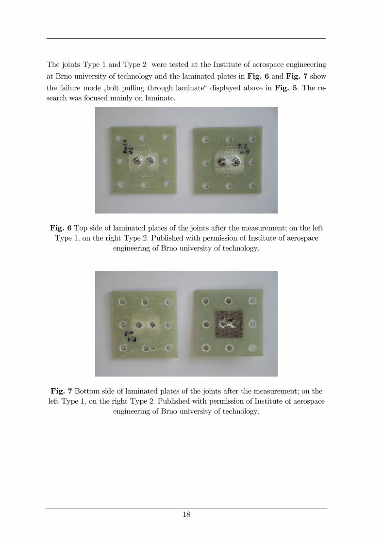
The joints Type 1 and Type 2 were tested at the Institute of aerospace engineeering
at Brno university of technology and the laminated plates in Fig. 6 and Fig. 7 show
the failure mode „bolt pulling through laminate“ displayed above in Fig. 5. The re-
search was focused mainly on laminate.
Fig. 6 Top side of laminated plates of the joints after the measurement; on the left
Type 1, on the right Type 2. Published with permission of Institute of aerospace
engineering of Brno university of technology.
Fig. 7 Bottom side of laminated plates of the joints after the measurement; on the
left Type 1, on the right Type 2. Published with permission of Institute of aerospace
engineering of Brno university of technology.
19
4 Research study
A progressive failure of bolted joints using the finite element method has been re-
searched along with an increasing of performace of computers and a progress in build-
ing of composite structures.
Adam, Bouvet, Castanié, Daidié and Bonhomme in [17] the pull-through phenomenon
firstly studied by simplified circular pull-through test method. The research extended
the Discrete Ply Model Method developed by Bouvet et al., where cohesive elements
were placed at the interfaces between solid elements to represent matrix cracks and
delamination, thus allowing the natural coupling between two damage modes. The
model showed good correalation with test results in terms of load-displacement curves
and prediction of the damage map until failure. Heimbs, Schmeer, Blaurock and Stee-
ger in 18] conducted test series of mechanically bolted joints with countersunk head
in quasi-isotropic carbon-epoxy composite laminate under quasi-static and dynamic
loads with velocities up to 10 m/s. The test campaign covered bolt pull-through tests,
single lap shear tests with one and two bolts and coach peel tests. No rate sensitivity
occurred for majority of test configurations, only the single lap shear tests with bolts
showed a change of failure mode at the highest test velocity enabling highest energy
absorption. Kabche, Caccese, Berube and Bragg in [19] presented an investigation of
the structural performance of hybrid composite-to-metal bolted joints loaded in flex-
ure, where the main goal was to develop a watertight, hybrid connection to resist
bending loads. Use of dobler plates and foam inserts in a bolted joint resulted in higher
strength and stiffness and can effectively mitigate joint opening, which improves the
ability to seal the joint and maintain watertight integrity. Kelly and Hagström in [20]
investigated experimentally and numerically a behavior of composites laminates sub-
jected to transverse load. Damage was found to initiate at low load levels, typically
20-30 % of the failure load. The dominant initial failure mode was matrix intralaminar
shear failure which occurred in sub-surface plies. The results from the finite element
model were found to be in general agreement with experimental observations. Cata-
lanotti, Camanho, Ghys and Marques in [21] presented an experimental and numerical
study of the fastener pull-through failure mode in flass-fiber reinforced plastic lami-
nates using both phenolic and vinylester resins. There is shown that the type of resin
does not affect the mechanical response of the joint when a pull-through test is per-
formed because similar values of the subcritical initial and final failure loads were
obtained. The prediction of the sub-critical initial failure load was performed using
three-dimensional finite element model where cohesive elements were used to simulate
delamination, because it was observed that the main failure mechanism was the de-
lamination. Elder, Verdaasdonk and Thomson in [2218] considered the capability of
finite element modelling to predict fastener pull-through failure of composite laminates,
which is dominated by inter-ply delamination and through-thickness shear failure of
the laminate. They used the LS-DYNA software for the study and found out that the
use of simplified FE models does have merit in modelling fastener pull-through pro-
vided the material quasi-isotropic and the boundary conditions are uniform around a
20
circular perimeter. Stocchi, Robinson and Thomson [23] dealt with analysis of single
lap shear composite joint with countersunk fasteners under static tensile load. In the
analysis he studied the influence of clamping force, coefficient of friction and clearance
on the joint behavior and fount that the model is able to identify correctly the joint
critical locations. Camanho and Matthews [24] studied a joint behavior of single and
multi-fastener joints in order to predict failure. He concluded that “there is no general
method that should be used to predict failure, but progressive damage models are quite
promising since important aspect of joint’s behavior can be modelled using this ap-
proach.” Moreover, he claims that “the use of three-dimensional models is suggested
with appropriate three-dimensional failure criterion and property degradation law.” C.
T. McCarthy with M. A. McCarthy in [25] analysed a 3D progressive damage finite
element model of multi-bolt, double-lap composite joints developed in the non-linear
finite element code Abaqus.” They studied the effects of variable bolt-hole clearance
and found out that clearance can cause major changes in the load distribution and
damage mechanism in the joint and it can lead to a significant reduction in the load
at which initial failure occurs. Wang, Zhou, Wu and Zhou [26] used extended finite
element method (XFEM) to predict failure of single-lap bolted joint. Hühne, Zerbst,
Kuhlman and Rolfes in [27] investigated a structural behavior of a single-lap, single-
bolt composite joint using three-dimensional finite element model and in contrast to
previous investigations, a influence of a liquid shim layer added between two laminates
on structural behavior of the joints was studied. As a first approach was used Hashin
three-dimensional failure criterion and a constant degradation model and it led to very
convervative results after validation with experimental data. As a second approach
they improved the model using a continuos degradation model and discover very good
correlation with the experimental data. Mouritz [28] reviewed published research into
polymer composite laminates reinforced in the through-thickness direction with z-pin.
In the paper research into the manufacture, microstructure, delamination resistance,
damage tolerance, joint strength and mechanical properties of z-pinnned composites is
described. Z-pinning can improve interlaminar toughness, impact damage resistance,
post-impact damage tolerance and through-thickness properties. The paper also de-
scribes the adverse effects of z-pins on the in-plane mechanical properties.
According to the papers can be claimed the following:
no general method exists that should be used to predict failure, but progressive
damage models are quite promising since important aspect of joint’s behavior
can be modelled using this approach,
the type of resin does not affect the mechanical response of the joint when a
pull-through test is performed,
Z-pinning can improve interlaminar toughness, impact damage resistance, post-
impact damage tolerance and through-thickness properties,
negative effects of z-pins are reduced elastic modulus, strength and fatigue per-
formance;
mechanical properties of laminate with z-pins depend on size and locations of
the pins.
21
5 Mechanics of composite materials
The most used materials these days are isotropic and homogeneus material (steel,
aluminium alloys etc). In contrast, due to increase in reliability and decrease of cost,
composite materials are used more and more. Composite materials are usually inho-
mogeneus and nonisotropic (orthotropic, anisotropic) unlike metals. An orthotropic
material can be described as a material with three different properties in three perpen-
dicular directions.[6]
Fig. 8 Comparison of behaviour of isotropic, orthotropic and anisotropic material.
[6]
5.1 Constitutive equations for an orthotropic material
Hooke’s law for linear elastic orthotropic material can be described as
𝜎1𝜎2𝜎3𝜏23𝜏31𝜏12
=
𝐶11 𝐶12 𝐶13 0 0 0𝐶21 𝐶22 𝐶23 0 0 0𝐶31 𝐶33 𝐶33 0 0 00 0 0 𝐶44 0 00 0 0 0 𝐶55 00 0 0 0 0 𝐶66
∙
휀1휀2휀3𝛾23𝛾31𝛾12
(5.1)
where 𝜎𝑖…component of normal stress, where i = 1, 2, 3
𝜏𝑖𝑗…component of shear stress, where i, j and i, j = 1, 2, 3
휀𝑖…component of normal strain, where i = 1, 2, 3
𝛾𝑖𝑗… component of shear strain, where i, j and i, j = 1, 2, 3
𝐶𝑖𝑗…component of stiffness matrix C, where i, j = 1, 2, 3, 4, 5, 6
22
Inverse Hooke’s law for linear elastic orthotropic material is given by
휀11휀22휀33𝛾23𝛾31𝛾12
=
𝑆11 𝑆12 𝑆13 0 0 0𝑆21 𝑆22 𝑆23 0 0 0𝑆31 𝑆33 𝑆33 0 0 00 0 0 𝑆44 0 00 0 0 0 𝑆55 00 0 0 0 0 𝑆66
∙
𝜎11𝜎22𝜎33𝜏23𝜏31𝜏12
where 𝑆𝑖𝑗…component of compliance matrix S, where i, j = 1, 2, 3,
4, 5, 6.
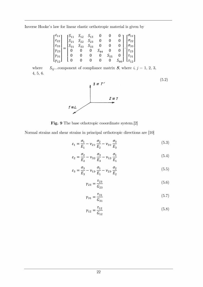
Fig. 9 The base othotropic cooordinate system.[2]
(5.2)
Normal strains and shear strains in principal orthotropic directions are [10]
휀1 =𝜎1𝐸1
− 𝜈21∙𝜎2𝐸2
− 𝜈31∙𝜎3𝐸3
(5.3)
휀2 =𝜎2𝐸2
− 𝜈32∙𝜎3𝐸3
− 𝜈12∙𝜎1𝐸1
(5.4)
휀3 =𝜎3𝐸3
− 𝜈13∙𝜎1𝐸1
− 𝜈23∙𝜎2𝐸2
(5.5)
𝛾23 =𝜏23𝐺23
(5.6)
𝛾31 =𝜏31𝐺31
(5.7)
𝛾12 =𝜏12𝐺12
(5.8)
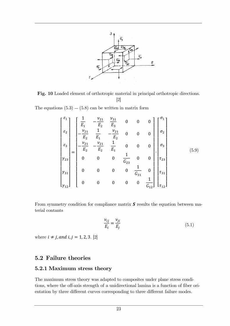
23
Fig. 10 Loaded element of orthotropic material in principal orthotropic directions.
[2]
The equations (5.3) ― (5.8) can be written in matrix form
휀1
휀2
휀3
𝛾23
𝛾31
𝛾12
=
1
𝐸1−𝜈21𝐸2
𝜈31𝐸3
0 0 0
−𝜈21𝐸2
1
𝐸1−𝜈21𝐸2
0 0 0
−𝜈21𝐸2
−𝜈21𝐸2
1
𝐸10 0 0
0 0 01
𝐺230 0
0 0 0 01
𝐺310
0 0 0 0 01
𝐺12
∙
𝜎1
𝜎2
𝜎3
𝜏23
𝜏31
𝜏12
(5.9)
From symmetry condition for compliance matrix 𝑺 results the equation between ma-
terial contants
𝜈𝑖𝑗
𝐸𝑖=
𝜈𝑗𝑖
𝐸𝑗 (5.1)
where 𝑖 ≠ 𝑗, 𝑎𝑛𝑑 𝑖, 𝑗 = 1, 2, 3. [2]
5.2 Failure theories
5.2.1 Maximum stress theory
The maximum stress theory was adapted to composites under plane stress condi-
tions, where the off-axis strength of a unidirectional lamina is a function of fiber ori-
entation by three different curves corresponding to three different failure modes.
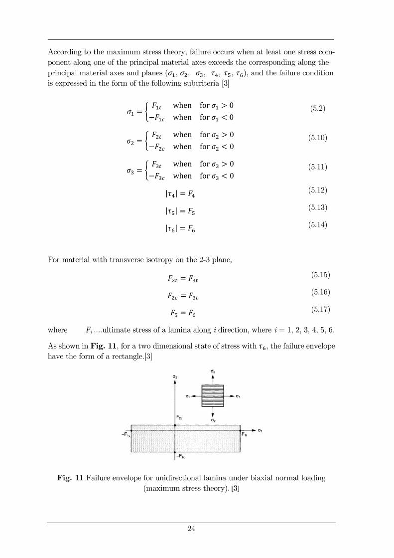
24
According to the maximum stress theory, failure occurs when at least one stress com-
ponent along one of the principal material axes exceeds the corresponding along the
principal material axes and planes (𝜎1, 𝜎2, 𝜎3, 𝜏4, 𝜏5, 𝜏6), and the failure condition
is expressed in the form of the following subcriteria [3]
𝜎1 = 𝐹1𝑡 when for 𝜎1 > 0
−𝐹1𝑐 when for 𝜎1 < 0 (5.2)
𝜎2 = 𝐹2𝑡 when for 𝜎2 > 0
−𝐹2𝑐 when for 𝜎2 < 0 (5.10)
𝜎3 = 𝐹3𝑡 when for 𝜎3 > 0
−𝐹3𝑐 when for 𝜎3 < 0 (5.11)
𝜏4 = 𝐹4 (5.12)
𝜏5 = 𝐹5 (5.13)
𝜏6 = 𝐹6 (5.14)
For material with transverse isotropy on the 2-3 plane,
𝐹2𝑡 = 𝐹3𝑡 (5.15)
𝐹2𝑐 = 𝐹3𝑡 (5.16)
𝐹5 = 𝐹6 (5.17)
where Fi ….ultimate stress of a lamina along i direction, where i = 1, 2, 3, 4, 5, 6.
As shown in Fig. 11, for a two dimensional state of stress with 𝜏6, the failure envelope
have the form of a rectangle.[3]
Fig. 11 Failure envelope for unidirectional lamina under biaxial normal loading
(maximum stress theory). [3]
25
5.2.2 Energy based interaction theory (Tsai-Hill)
The deviatoric or distortional energy has been proposed by many investigators (e.g.,
von Mises, Hencky, Nadai, Novozhilov) in various forms as a failure criterion for iso-
tropic ductile metals. For a two-dimensional state of stress referred to the principal
stress directions, the von Mises yield criterion has the form [3]
𝜎12 + 𝜎1
2 − 𝜎1𝜎2 = 𝜎𝑦𝑝2 (5.18)
where 𝜎𝑦𝑝 is the yield stress.
The following criterion for ductile metals with anisotropy was proposed by Hill
𝐴𝜎12 + 𝐵𝜎1
2 − 𝐶𝜎1𝜎2 + 𝐷𝜏62 = 1 (5.19)
where A, B, C, and D are material parameters characteristic of the current state
of anisotropy.
For uniaxial longitudinal loading to failure, 𝜎2𝑢 = 𝐹1, 𝜎2 = 𝜏6 = 0 and the equation
above yields
𝐴 =1
𝐹12
(5.20)
For uniaxial transverse loading to failure, 𝜎2𝑢 = 𝐹2, 𝜎1 = 𝜏6 = 0 and the equation
(5.19) yields
𝐵 =1
𝐹22
(5.21)
For in-plane shear loading to failure, 𝜎1 = 𝜎2 = 0, 𝜏6𝑢 = 𝐹6 and the equation (5.19)
𝐷 =1
𝐹62
(5.22)
The superscript u in the above denotes the ultimate value of stress at failure. Since
failure will occur when the transverse stress 𝜎2 reaches the transverse strength value
𝐹2, which is much lower than the longitudinal strength 𝐹1, the equation (5.19) then
yields [3]
𝐶 = −1
𝐹12 (5.23)
The Tsai-Hill criterion for a two-dimensional state of stress is given by substituting A,
B, C and D into (5.19)
𝜎12
𝐹12 +
𝜎22
𝐹22 +
𝜏62
𝐹62 −
𝜎1𝜎2
𝐹12 = 1
(5.24)
26
The appropriate strength values can be used in the equation above according to the
signs of the normal stresses 𝜎1 and 𝜎2, because there is no distinction between tensile
and compressive strengths, hence
𝐹1 = 𝐹1𝑡 when 𝜎1 > 0𝐹1𝑐 when 𝜎1 > 0
(5.25)
𝐹2 = 𝐹2𝑡 when 𝜎2 > 0𝐹2𝑐 when 𝜎2 > 0
(5.26)
As F2 ≈ F3 and F5 ≈ F6, the failure criterion for three-dimensional state of stress is
𝜎12
𝐹12 +
𝜎22 + 𝜎3
2
𝐹22 +
𝜏42
𝐹42 +
𝜏52 + 𝜏6
2
𝐹52 −
𝜎1𝜎2
𝐹42 −
𝜎1𝜎2
𝐹42 = 1
(5.27)
or
𝜎12 − 𝜎1𝜎2 − 𝜎1𝜎3
𝐹12 +
𝜎22 + 𝜎3
2 − 𝜎2𝜎3
𝐹12 +
𝜏42
𝐹42 +
𝜏52 + 𝜏6
2
𝐹52 = 1
(5.28)
The theory is based on Hill’s theory, which is suitable for homogeneous, anisotropic
and ductile material, however, composites are mostly heterogeneous and brittle.
5.2.3 Interactive tensor polynomial theory (Tsai-Wu)
Tsai and Wu [3][16] developed a modified tensor polynomial theory by assuming the
existence of a failure surface in expanded form
𝑓1𝜎1 + 𝑓2𝜎2 + 𝑓3𝜎3 + 𝑓4𝜏4 + 𝑓5𝜏5 + 𝑓6𝜏6 + 𝑓11𝜎1
2 + 𝑓22𝜎22 + 𝑓33𝜎3
2
+ 𝑓44𝜏42 +
+𝑓55𝜏52 + 𝑓66𝜏6
2 + 2𝑓12𝜎2 + 2𝑓13𝜎3 + 2𝑓14𝜏4 + 2𝑓15𝜏5 + 2𝑓16𝜏6+ 2𝑓23𝜎2𝜎3 +
+2𝑓24𝜎2𝜏4 + 2𝑓25𝜎2𝜏5 + 2𝑓36𝜎3𝜏6 + 2𝑓45𝜏4𝜏5 + 2𝑓46𝜏4𝜏6 + 2𝑓56𝜏5𝜏6= 1
(5.29)
where 𝑓𝑖 , 𝑓𝑖𝑗 are second order and fourth strength tensors, and 𝑖, 𝑗 = 1, 2, … , 6. [3]
All linear terms in the shear stresses and all terms associated with interaction of normal
and shear stresses and between shear stresses acting on different planes are omitted,
because the shear strength of a unidirectional composite, F4, F5 and F6 reffered to the
principal material planes ar independant of the sign of the shear stress (τ4, τ5, τ6). [3]
−𝑓4 = 𝑓5 = 𝑓6 = 𝑓14 = 𝑓15 = 𝑓16 = 𝑓24 = 𝑓25 = 𝑓26 = 𝑓34 = 𝑓35 = 𝑓36
= 𝑓45 =
= 𝑓46 = 𝑓56 = 0
(5.30)
If transverse isotropy in the 2-3 plane is assumed, the number of coefficient is reduced,
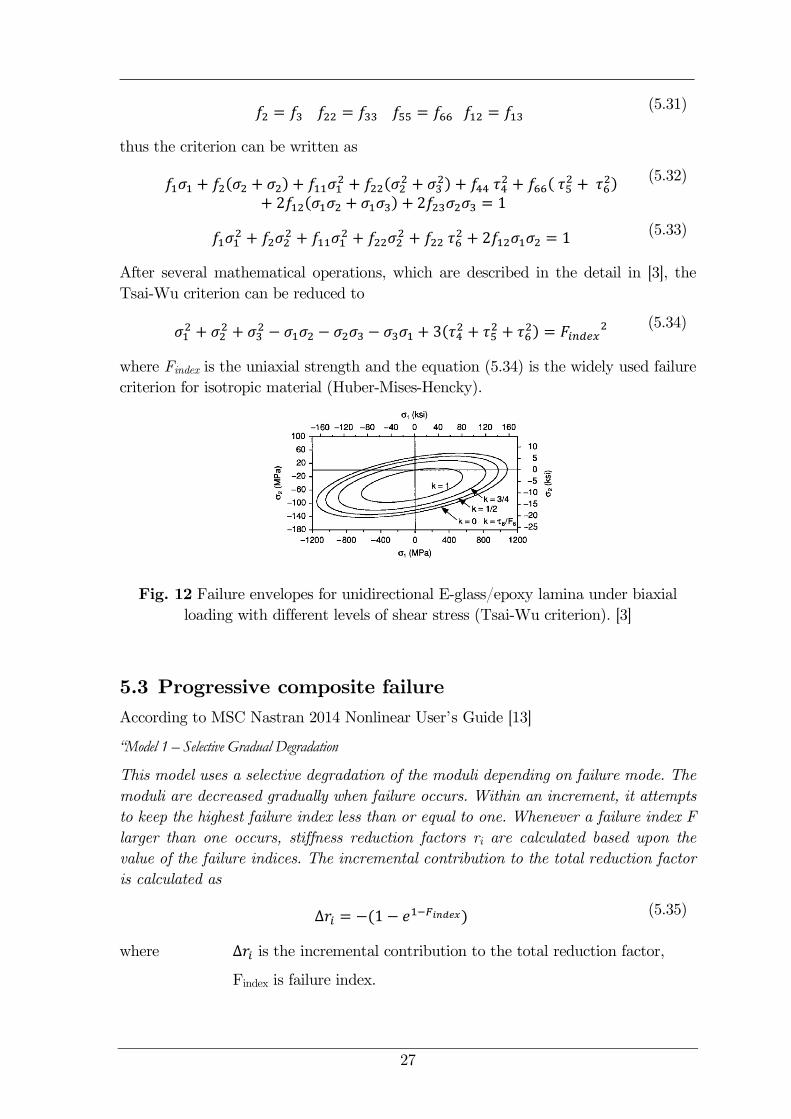
27
𝑓2 = 𝑓3 𝑓22 = 𝑓33 𝑓55 = 𝑓66 𝑓12 = 𝑓13
(5.31)
thus the criterion can be written as
𝑓1𝜎1 + 𝑓2 𝜎2 + 𝜎2 + 𝑓11𝜎1
2 + 𝑓22 𝜎22 + 𝜎3
2 + 𝑓44 𝜏42 + 𝑓66 𝜏5
2 + 𝜏62
+ 2𝑓12 𝜎1𝜎2 + 𝜎1𝜎3 + 2𝑓23𝜎2𝜎3 = 1
(5.32)
𝑓1𝜎1
2 + 𝑓2𝜎22 + 𝑓11𝜎1
2 + 𝑓22𝜎22 + 𝑓22 𝜏6
2 + 2𝑓12𝜎1𝜎2 = 1 (5.33)
After several mathematical operations, which are described in the detail in [3], the
Tsai-Wu criterion can be reduced to
𝜎12 + 𝜎2
2 + 𝜎32 − 𝜎1𝜎2 − 𝜎2𝜎3 − 𝜎3𝜎1 + 3 𝜏4
2 + 𝜏52 + 𝜏6
2 = 𝐹𝑖𝑛𝑑𝑒𝑥2
(5.34)
where Findex is the uniaxial strength and the equation (5.34) is the widely used failure
criterion for isotropic material (Huber-Mises-Hencky).
Fig. 12 Failure envelopes for unidirectional E-glass/epoxy lamina under biaxial
loading with different levels of shear stress (Tsai-Wu criterion). [3]
5.3 Progressive composite failure
According to MSC Nastran 2014 Nonlinear User’s Guide [13]
“Model 1 – Selective Gradual Degradation
This model uses a selective degradation of the moduli depending on failure mode. The
moduli are decreased gradually when failure occurs. Within an increment, it attempts
to keep the highest failure index less than or equal to one. Whenever a failure index F
larger than one occurs, stiffness reduction factors ri are calculated based upon the
value of the failure indices. The incremental contribution to the total reduction factor
is calculated as
Δ𝑟𝑖 = − 1 − 𝑒1−𝐹𝑖𝑛𝑑𝑒𝑥 (5.35)
where Δ𝑟𝑖 is the incremental contribution to the total reduction factor,
Findex is failure index.
28
This is done differently for different failure criteria as described below. Six such re-
duction factors are stored and updated. They are then used for scaling the respective
material modulus according to
𝐸11𝑛𝑒𝑤 = 𝑟1𝐸11
𝑜𝑟𝑖𝑔
(5.36)
𝐸22𝑛𝑒𝑤 = 𝑟2𝐸22
𝑜𝑟𝑖𝑔 (5.37)
𝐸33𝑛𝑒𝑤 = 𝑟3𝐸33
𝑜𝑟𝑖𝑔
(5.38)
𝐺12𝑛𝑒𝑤 = 𝑟4𝐺12
𝑜𝑟𝑖𝑔
(5.39)
𝐺23𝑛𝑒𝑤 = 𝑟5𝐺23
𝑜𝑟𝑖𝑔
(5.40)
𝐺31𝑛𝑒𝑤 = 𝑟6𝐺31
𝑜𝑟𝑖𝑔
(5.41)
The Poisson’s ratios are scaled in the same way as the corresponding shear modulus.
For the maximum stress and maximum strain criteria the reduction factors are calcu-
lated separately from each separate failure index: r1 is calculated from the first failure
index as given by equation (5.36) above, r2 is calculated from the second failure index
from equation (5.37) etc. Thus, there is no coupling of the different failure modes for
these criteria. For the failure criteria which only have one failure index: Tsai-Wu,
Hoffman and Hill, all six reduction factors are decreased in the same way, using the
smallest of the ri.“ [13]
5.4 Strengh ratio
Since failure indices Findex are in general nonlinear functions (except for the maximum
stress and strain failure theories), thus they do not determine how far is to failure and
hence strength ratio is a better indicator. Strength ratio SR is similar to margin of
safety and is described using equation
𝑆𝑅 =allowable loads
actual loads. (5.42)
Table 1 Comparison of failure index and strength ratio.
Indicator Failure condition
Failure index Findex > 1
Strength ratio SR < 1

29
For example, the determination of strength ratio will be showed using Tsai-Wu crite-
ria.
𝐹𝑖𝑛𝑑𝑒𝑥 = 𝜎12
𝑋𝑇𝑋𝑐+
𝜎22
𝑌𝑇𝑌𝑐+ 2𝐹12𝜎1𝜎2 +
𝜏122
𝑆2+ 𝜎1
1
𝑋𝑇−
1
𝑋𝐶 + 𝜎2
1
𝑌𝑇−
1
𝑌𝑐 (5.43)
Actual stresses were substituted with the product (𝑆𝑅 ⋅ 𝑎𝑐𝑡𝑢𝑎𝑙𝑙 𝑠𝑡𝑟𝑒𝑠𝑠 and set Findex
= 1, thus the equation will be
0 = 𝜎12
𝑋𝑇𝑋𝑐+
𝜎22
𝑌𝑇𝑌𝑐+ 2𝐹12𝜎1𝜎2 +
𝜏122
𝑆2 𝑆𝑅2 + 𝜎1
1
𝑋𝑇−
1
𝑋𝐶 + 𝜎2
1
𝑌𝑇−
1
𝑌𝑐 𝑆𝑅 − 1 (5.44)
As the equation (5.44) is quadratic, strength ratio will be determined solving for roots
𝑆𝑅. [31]
When at certain failure index Findex = 19,2287 is strength ratio SR = 0,228, this indi-
cates that the load is too high by a factor of
1
𝑆𝑅=
1
0,228= 4,39
(5.45)
Allowable load can be obtained dividing actual load by 4,39 or multiplying by strength
ratio SR = 0,228. [31]
30
6 Solution method
6.1 The finite element method
The finite element method provides numerical solution of field problems. An essence
of the method consists of a dividing a structure into finite number of elements, which
are connected using nodes. The process of dividing the structure is called discretiza-
tion. Degrees of freedom, defined in nodes, are refered to as unknown parameters. A
functional dependence between the unknown parameters in the elements and nodes
is given by a basis function. This greatly simplifies the mathematical description of
complex shapes and replaces it with a description of basic geometric shapes such as
rectangles, triangles or quads. This replaces the job search function continuous deter-
mination of the final number of unknown parameters to the search function interpo-
lation. This treatment is called continuous to discrete problem. Discrete problem is
then solved by means of algebraic finite number of steps using computer technology.
Basic approaches to solving the system of equations can be divided according to sev-
eral criteria. In terms of mathematical description of the problem distinguish the ap-
proaches to the differential and variation. Differential approach is to build a system
of differential equations. Variational approach based on the observation that the pro-
cesses occurring in nature have such a story, that of all the opportunities that may
arise, to implement processes are minimized. The principle of this approach, there-
fore, is to find the functions for which it becomes functional a stationary value. Vari-
ational approach is referred to as energy and is used primarily in conjunction with
numerical methods and FEM. When implementing the solution, it is possible to use
either analytical or numerical solutions. If the task is solved analytically, the aim of
finding a solution in the form of continuous functions using the methods of mathe-
matical analysis. Numerical solution lies in continuous to discrete problem, as de-
scribed in a previous paragraphs, and the solution of algebraic equations. Nowadays,
the use of FEM as a numerical method in most cases carried out using variational
formulation and deformation approach. The primary unknown functions are func-
tions of displacements. [4]
The deformation variant of FEM is the Lagrange variational principle: Only func-
tions which give a stationary value of total potential energy Π are realized of all
functions of displacements preserving continuity of body and meeting the geometric
boundary conditions." It is proven that the stationary value exists and its minimum
is the functional Π.
Equation (6.1) expresses the total potential energy Π as difference of stress energy W
and the potential of the external load P. [4]
𝛱 = 𝑊 − 𝑃 (6.1)
31
The strain energy of the body Ω is given by equation
𝑊 =
1
2 𝝈𝑇𝜖 𝑑𝑉
⬚
Ω
(6.2)
and the potential energy of the external load P
𝑃 = 𝒖𝑇𝒐 𝑑𝑉 + 𝒖𝑇𝒑 𝑑𝑆
⬚
Γ𝑝
⬚
Ω
(6.3)
In this relationship the following column matrices are used
- displacements 𝒖𝑇 = [𝑢, 𝑣, 𝑤] (6.4)
- strains 𝝐𝑇 = 𝜖𝑥, 𝜖𝑦, 𝜖𝑧 , 𝛾𝑥𝑦, 𝛾𝑦𝑧 , 𝛾𝑧𝑥 (6.5)
- stresses 𝝈𝑇 = 𝜎𝑥, 𝜎𝑦, 𝜎𝑧 , 𝜏𝑥𝑦, 𝜏𝑦𝑧, 𝜏𝑧𝑥 (6.6)
- distributed body
forces 𝒖𝑇 = 𝑜𝑥, 𝑜𝑦, 𝑜𝑧 (6.7)
- surface forces 𝒑𝑇 = 𝑝𝑥, 𝑝𝑦, 𝑝𝑧 (6.8)
After substituting the global stiffness matrix, the total strain energy can be expressed
as follows [4]:
𝑊 =
1
2𝑼𝑇𝑲1𝑼 (6.9)
Similarly, after the representation of the overall matrix F, the external load leads to:
𝑷 = 𝑼𝑇𝑭 (6.10)
Substituting equation (6.9) and (6.10) in equation for the total potential energy Π
(6.11), we obtain
Π =
1
2𝑼𝑻𝑲𝑼− 𝑼𝑻𝑭
(6.11)
The stationary value of the functional Π according to the Lagrange variational prin-
ciple:
𝜕Π
𝜕𝑼= 0
(6.12)
32
Finally, from the partial derivatives according to u1, u2, u3, u4 we obtain a system of
linear equations [4]:
𝑲𝑼 = 𝑭 (6.13)
This equation is called the basic equation of the finite element method.
6.2 Nonlinear solution
In general, three causes of nonlinear behaviour exist
a) large displacements – a change of geometrical configuration during loading
b) material nonlinearity - plasticity, viscous behaviour
c) contact – a change of touching area. [30]
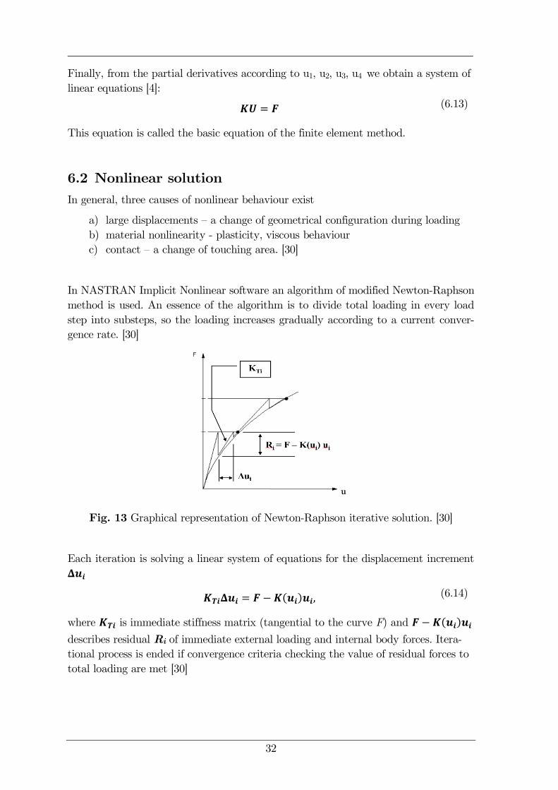
In NASTRAN Implicit Nonlinear software an algorithm of modified Newton-Raphson
method is used. An essence of the algorithm is to divide total loading in every load
step into substeps, so the loading increases gradually according to a current conver-
gence rate. [30]
Fig. 13 Graphical representation of Newton-Raphson iterative solution. [30]
Each iteration is solving a linear system of equations for the displacement increment
𝚫𝒖𝒊
𝑲𝑻𝒊𝚫𝒖𝒊 = 𝑭 −𝑲 𝒖𝒊 𝒖𝒊, (6.14)
where 𝑲𝑻𝒊 is immediate stiffness matrix (tangential to the curve F) and 𝑭 − 𝑲 𝒖𝒊 𝒖𝒊
describes residual Ri of immediate external loading and internal body forces. Itera-
tional process is ended if convergence criteria checking the value of residual forces to
total loading are met [30]
33
𝑅𝑖
𝐹𝑡𝑜𝑡𝑎𝑙≤ 𝛿𝐹 (6.15)
Similarly, the value of displacement increment can be checked
Δ𝑢𝑖
𝑢𝑡𝑜𝑡𝑎𝑙≤ 𝛿𝑢 (6.16)
compared with the given tolerances 𝛿𝐹, 𝛿𝑢. [30]
6.3 Continuum mechanics
Nowadays, two types of description of the motion of a continuum are mostly used:
1. Referential description, where the position X of the particle in a chosen refer-
ence configuration and the time are independant variables. The description is
called the Lagrangian description when the reference configuration is cho-
sen to bet he actual initial state at t = 0. The unstressed state is usually cho-
sen to be the reference configuration.
2. Relative description, where the present position x and occupied by the parti-
cle at time t and the present time t are independent variables. The description
is most used in fluid mechanics, sometimes calles the Eulerian descrip-
tion.[5]
Lagrangian description can be written symbolically
𝑥 = 𝑥 𝑋, 𝑡 (6.17)
with Cartesian components
𝑥𝑟 = 𝑥𝑟 𝑋1, 𝑋2, 𝑋3, 𝑡 (6.18)
where 𝑋1, 𝑋2, 𝑋3 are the material cooordinates of the particle.[5]
For determination stresses and strains at nonlinear analyses the following stress and
stress tensor are used.
Green-Lagrange strain tensor is related to underformed coordinates but rotation of
the element is respected. [29]
𝐸𝑖𝑗𝐿 =
1
2 𝜕𝑢𝑖
𝜕𝑋𝑗+𝜕𝑢𝑗
𝜕𝑋𝑖+𝜕𝑢𝑘
𝜕𝑋𝑗
𝜕𝑢𝑘
𝜕𝑋𝑖 (6.19)
34
Almansi-Hamel strain tensor is related to undeformed coordinates.[29]
𝐸𝑖𝑗𝐴 =
1
2 𝜕𝑢𝑖
𝜕𝑥𝑗+𝜕𝑢𝑗
𝜕𝑥𝑖−𝜕𝑢𝑘
𝜕𝑥𝑗
𝜕𝑢𝑘
𝜕𝑥𝑖 (6.20)
Cauchy logarithmic strain tensor uses the infinitesimal increment and current length
unlike Green-Lagrange and Almansi-Hamel strain tensor. [29]
𝐸𝑖𝐶 =
𝑑𝑥𝑖𝑥𝑖
𝑥𝑖𝑘
𝑋𝑖0
= ln 𝑥 𝑋𝑖0
𝑥𝑖𝑘 = ln 𝑥𝑖𝑘 − ln𝑋𝑖0 = ln 𝑥𝑖𝑘𝑋𝑖0
= ln 𝜆𝑖 (6.21)
Cauchy stress tensor (Euler’s stress tensor, true stress) is given by the derivation of a
true elementary force and a true deformed area of an element.[29]
𝜎𝑖 =𝑑𝐹𝑖
𝑑𝑥𝑗𝑑𝑥𝑘 (6.22)
The first Piola-Kirchhoff stress tensor (Lagrange stress tensor, engineering stress) is
given by the derivation of a the true elementary force and undeformed area of the
element.[29]
𝜏𝑖 =𝑑𝐹𝑖
𝑑𝑋𝑗𝑑𝑋𝑘 (6.23)
The second Piola-Kirchhoff stress tensor is given by the derivation of an elementery
force 𝑑𝐹0𝑖 and undeformed area of an element. The tensor is without exact physical
meaning, but i tis symmetric energy conjucated with Green-Lagrange strain tensor for
large strains. The force 𝑑𝐹0𝑖 is changed at loading of an element unlike the true force
in the same way as the elementary coordinate, which is changing according the follow-
ing equation [29]
𝑑𝑥𝑖 =𝑑𝑥𝑖𝑑𝑋𝑗
𝑑𝑋𝑗 (6.24)
For backward transformation to undeformed state the next formula is used
𝑑𝑥𝑖 =𝑑𝑥𝑖𝑑𝑋𝑗
𝑑𝑋𝑗 (6.25)
Finally, the stress is defined as
𝑑𝑆𝑖 =𝑑𝐹0𝑖
𝑑𝑋𝑗𝑑𝑋𝑗 (6.26)
35
7 Description of computional models and
settings of solution
All major solvers like Abaqus, Ansys and MSC Nastran and Marc allow the progressive
failure analysis of composite materials. Explicit solvers can be used too, but duration
of the analyses especially with solid elements can take extremely long time. One of the
most popular solvers these days, Abaqus, has programmed one failure criterion Hashin,
wich can be used only with shell and continuum shell elements. Since the use of Hashin
criterion with 3D solid elements is not available using GUI, a user has to write Abaqus
user-defined material model UMAT (Abaqus Standard) or VUMAT (Abaqus Ex-
plicit), where the criterion will be included. The progressive failure analysis introduced
in Ansys 14.0, has been extended in the following versions. Ansys has written the
failure criteria and they can be used with solid 3D elements as well as with shell
elements. In MAPDL, input and post – processing must be performed via commands,
no GUI input is available. In Workbench, material input and post-processing is avail-
able, and the damage evolution law – continuum damage mechanics was finally added
in version 17.0. Similarly as Ansys, Nastran Implicit Nonlinear as well as Marc have
programmed several failure criteria, which can be used with solid 3D elements as well
as with shell elements.
Several trial analysis were done using implicit solver Ansys, implicit solver Abaqus
Standard, implicit solver Nastran SOL400 and explicit solver Abaqus Explicit. The
trial analysis using explicit solver Abaqus Explicit was done with medium complex
computional model with 4 elements through-thickness of the laminate, where solution
of time 0,0002 s of total time 1 s using quad core Intel Xeon 3,6 GHz processor lasted
unacceptable long time, thus the run was terminated. Explicit solver takes into account
density of material, hence the kinetic energy of the deformed material should not ex-
ceed 5 % of its internal energy because the experiments were quasi-static, and it leads
to long computation time. After discussion with my consultant at Institute of aero-
space engineering at Brno university of technology, the solver Nastran Implicit Non-
linear SOL 400 was chosen for the FE analyses. The reasons for choosing Nastran were
the following: acceptable computation times compared to explicit solver, availability
at Institute of aerospace engineering, the fact that Nastran has programmed several
failure criteria, which can be used for progressive failure analysis and the fact that it
is widely used for aircraft development.
36
Table 2 Comparison of capabilities of implicit and explicit solver.
property
nonlinear solver type
implicit explicit
post first-ply-failure behavior yes yes
prediction of ultimate load depends on geometry, mesh
and material model
yes
duration of analysis normal enormous
7.1 Geometry
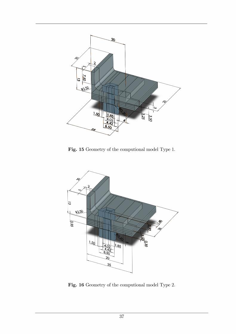
Due to two planes of symmetry, only one-quarter geometries of the joints were created
as shown in Fig. 14. The models (Fig. 15 and Fig. 16) were built and cut for pure
hexahedral meshing using the CAD system Solidworks and exported in STEP format.
Afterwards, the geometries were imported to Patran for further processing of the mod-
els. Since according to Mouritz [28] affects especially interlaminar properties, which
were not investigated in this work, z-pins of Type 2 were not modelled.
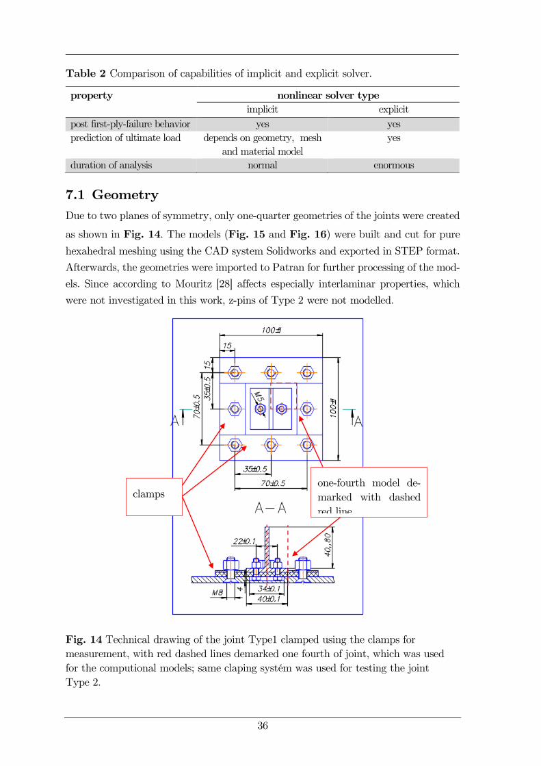
Fig. 14 Technical drawing of the joint Type1 clamped using the clamps for
measurement, with red dashed lines demarked one fourth of joint, which was used
for the computional models; same claping systém was used for testing the joint
Type 2.
one-fourth model de-
marked with dashed
red line
clamps
37
Fig. 15 Geometry of the computional model Type 1.
Fig. 16 Geometry of the computional model Type 2.
38
7.2 Mesh
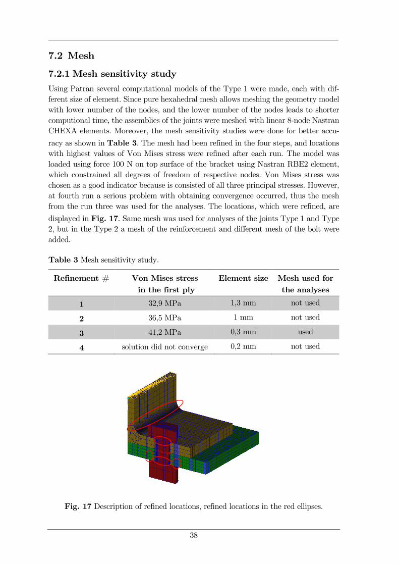
7.2.1 Mesh sensitivity study
Using Patran several computational models of the Type 1 were made, each with dif-
ferent size of element. Since pure hexahedral mesh allows meshing the geometry model
with lower number of the nodes, and the lower number of the nodes leads to shorter
computional time, the assemblies of the joints were meshed with linear 8-node Nastran
CHEXA elements. Moreover, the mesh sensitivity studies were done for better accu-
racy as shown in Table 3. The mesh had been refined in the four steps, and locations
with highest values of Von Mises stress were refined after each run. The model was
loaded using force 100 N on top surface of the bracket using Nastran RBE2 element,
which constrained all degrees of freedom of respective nodes. Von Mises stress was
chosen as a good indicator because is consisted of all three principal stresses. However,
at fourth run a serious problem with obtaining convergence occurred, thus the mesh
from the run three was used for the analyses. The locations, which were refined, are
displayed in Fig. 17. Same mesh was used for analyses of the joints Type 1 and Type
2, but in the Type 2 a mesh of the reinforcement and different mesh of the bolt were
added.
Table 3 Mesh sensitivity study.
Refinement # Von Mises stress
in the first ply
Element size Mesh used for
the analyses
1 32,9 MPa 1,3 mm not used
2 36,5 MPa 1 mm not used
3 41,2 MPa 0,3 mm used
4 solution did not converge 0,2 mm not used
Fig. 17 Description of refined locations, refined locations in the red ellipses.
39
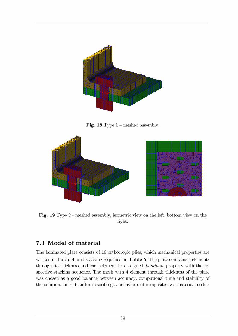
Fig. 18 Type 1 – meshed assembly.
Fig. 19 Type 2 - meshed assembly, isometric view on the left, bottom view on the
right.
7.3 Model of material
The laminated plate consists of 16 orthotropic plies, which mechanical properties are
written in Table 4. and stacking sequence in Table 5. The plate cointains 4 elements
through its thickness and each element has assigned Laminate property with the re-
spective stacking sequence. The mesh with 4 element through thickness of the plate
was chosen as a good balance between accuracy, computional time and stabililty of
the solution. In Patran for describing a behaviour of composite two material models
40
were chosen: Linear Elastic and Failure1 (SOL400/6000) as shown in Fig. 20. Orig-
inal material of the bracket was aluminium alloy D16, which is widely used for aircraft
building.
Table 4 Material properties of one lamina of glass fiber reinforced polymer.
Property Symbol Value Unit
Young’s modulus E11 39 600 MPa
Young’s modulus E22 20 600 MPa
Young’s modulus E33 3 000 MPa
Poisson’s s ratio ν12 = ν23 = ν13 0,26 -
Shear modulus G12 = G23 = G13 5 100 MPa
Longitudinal tensile strength F11t 578 MPa
Transverse tensile strength F22t 385 MPa
Transverse tensile/compressive
strength F33t= F33c 26 MPa
Transverse compressive strength F11c 462 MPa
Transverse compressive strength F22c 321 MPa
Shear strength F12 45 MPa
Shear strength F23= F13 22 MPa
Table 5 Stacking sequence.
Layer # Orientation (°) Layer # Orientation (°)
1 0 9 90
2 45 10 -45
3 -45 11 45
4 0 12 90
5 90 13 0
6 45 14 -45
7 -45 15 45
8 90 16 0
41
Table 6 Material properties of aluminium alloy D16.
Property Symbol Value Unit
Young’s modulus E 72 000 MPa
Poisson’s ratio ν 0,33 -
Yield point σyp 351 MPa
Hardening slope ET 1600 MPa
Table 7 Materials properties for steel of the bolt.
Property Symbol Value Unit
Young’s modulus E 207 000 MPa
Poisson’s ratio ν 0,3 -
Table 8 Material properties for steel of the reinforcement.
Property Symbol Value Unit
Young’s modulus E 207 000 MPa
Poisson’s ratio ν 0,3 -
Yield point σyp 500 MPa
Hardening slope ET 1600 MPa
7.3.1 Sensitivity study of residual stiffness factor
As the residual stiffness factor, which was described in detail in chapter 5.3, is an
important value for progressive failure analysis, the sensitivity study of the factor was
done using various values of the factor and computational model of the joint Type 2.
The results of the study are shown in Fig. 21. Similar study was done using the model
Type 1. In the first case (Type 2), a problem with obtaining convergence occurred
with values lower than 0,05 . In the case with the model Type 1 problems with ob-
taining convergence occurred with values lower than 0,15. As a good balance between
accuracy and stabililty of solution, the value of residual stiffness factor 0,15 was chosen
for both cases. According the study can be claimed the following statement:
“Too low values of residual stiffness factor can cause problems with achieving the
convergence, too high values can make the model too stiff, thus inaccurate.”

42
Fig. 20 Patran window for input strength limits, residual stiffness factor is in the
red box.
Fig. 21 Results of the sensitivity study of residual stiffness factor ri using the
computional model Type 2.
7.4 Model of boundary conditions
Due to symmetry two side surfaces of the whole assembly have assigned zero displace-
ment in x-direction and in y-direction, and two side surfaces of the laminated plate
were clamped. In adition, the model Type 2 has set symmetrical boundary conditions
in x-direction and in y-direction on two surfaces of the reinforcement. All the boundary
conditions are shown in Fig. 22.
43
Fig. 22 Boundary conditions.
7.5 Contacts
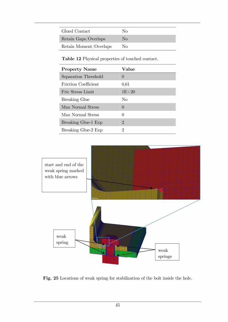
Nastran Implicit Nonlinear uses the concept of contact bodies, thus contacts were set
as shown in Table 9 and Table 10. Nonlinear touched contacts were used in both
cases with coefficient of friction f = 0,61, which was determined for friction between
steel and aluminium according to Shigley [8]. Example of values of geometrical and
physical properties, which were used in the analyses are shown in Table 11 and Table
12. In both cases a problem was with a stabilization of the bolt inside the hole, thus
achieving convergence, therefore the bolt was stabilized by four symmetrically located
weak springs with stiffness 50 N∙mm-1 as shown in Fig. 25.
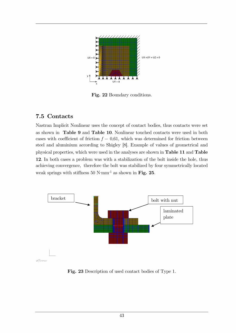
Fig. 23 Description of used contact bodies of Type 1.
bracket bolt with nut
laminated
plate
44
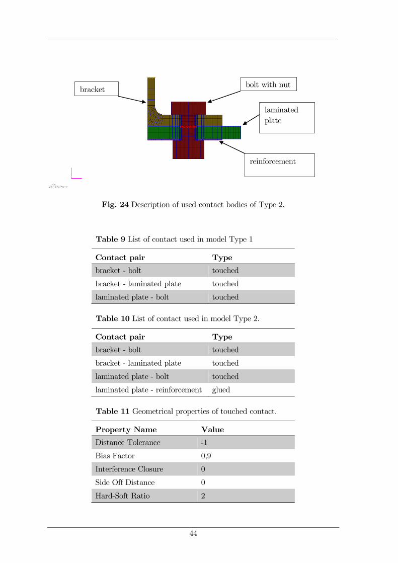
Fig. 24 Description of used contact bodies of Type 2.
Table 9 List of contact used in model Type 1
Contact pair Type
bracket - bolt touched
bracket - laminated plate touched
laminated plate - bolt touched
Table 10 List of contact used in model Type 2.
Contact pair Type
bracket - bolt touched
bracket - laminated plate touched
laminated plate - bolt touched
laminated plate - reinforcement glued
Table 11 Geometrical properties of touched contact.
Property Name Value
Distance Tolerance -1
Bias Factor 0,9
Interference Closure 0
Side Off Distance 0
Hard-Soft Ratio 2
bolt with nut
laminated
plate
bracket
reinforcement
45
Glued Contact No
Retain Gaps/Overlaps No
Retain Moment/Overlaps No
Table 12 Physical properties of touched contact.
Property Name Value
Separation Threshold 0
Friction Coefficient 0,61
Fric Stress Limit 1E+20
Breaking Glue No
Max Normal Stress 0
Max Normal Stress 0
Breaking Glue-1 Exp 2
Breaking Glue-2 Exp 2
Fig. 25 Locations of weak spring for stabilization of the bolt inside the hole.
weak
spring
weak
springs
start and end of the
weak spring marked
with blue arrows
46
7.6 Model of loads
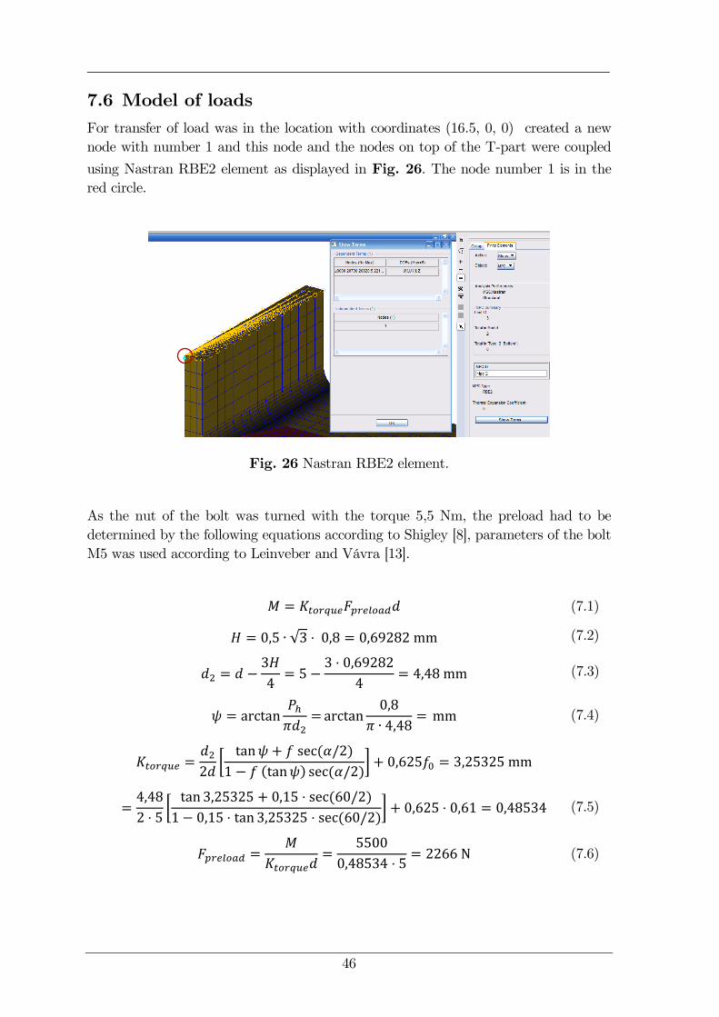
For transfer of load was in the location with coordinates (16.5, 0, 0) created a new
node with number 1 and this node and the nodes on top of the T-part were coupled
using Nastran RBE2 element as displayed in Fig. 26. The node number 1 is in the
red circle.
Fig. 26 Nastran RBE2 element.
As the nut of the bolt was turned with the torque 5,5 Nm, the preload had to be
determined by the following equations according to Shigley [8], parameters of the bolt
M5 was used according to Leinveber and Vávra [13].
𝑀 = 𝐾𝑡𝑜𝑟𝑞𝑢𝑒𝐹𝑝𝑟𝑒𝑙𝑜𝑎𝑑𝑑 (7.1)
𝐻 = 0,5 ∙ 3 ⋅ 0,8 = 0,69282 mm (7.2)
𝑑2 = 𝑑 −3𝐻
4= 5 −
3 ⋅ 0,69282
4= 4,48 mm (7.3)
𝜓 = arctan𝑃ℎ𝜋𝑑2
=arctan0,8
𝜋 ∙ 4,48= mm (7.4)
𝐾𝑡𝑜𝑟𝑞𝑢𝑒 =𝑑2
2𝑑
tan𝜓 + 𝑓 sec 𝛼/2
1 − 𝑓 tan𝜓 sec 𝛼/2 + 0,625𝑓0 = 3,25325 mm
=4,48
2 ⋅ 5
tan 3,25325 + 0,15 ⋅ sec 60/2
1 − 0,15 ⋅ tan 3,25325 ⋅ sec 60/2 + 0,625 ⋅ 0,61 = 0,48534 (7.5)
𝐹𝑝𝑟𝑒𝑙𝑜𝑎𝑑 =𝑀
𝐾𝑡𝑜𝑟𝑞𝑢𝑒𝑑=
5500
0,48534 ⋅ 5= 2266 N (7.6)
47
where
𝑀 (mm) torque,
𝐾𝑡𝑜𝑟𝑞𝑢𝑒 (―) coefficient of the torque,
𝑑 (mm) diameter of the thread,
𝑑2 (mm) pitch diameter of the thread,
𝐻 (mm) height of the thread triangle
𝐹𝑝𝑟𝑒𝑙𝑜𝑎𝑑 (N) preload,
𝑓0 (―) coefficient of friction between nut and surface of
the joined part, in this case friction occurs between
steel and aluminium, thus according to [8]
𝑓0 = 0,61 𝑓 (―) coefficient of friction between threads, according to
[8] 𝑓 = 0,15
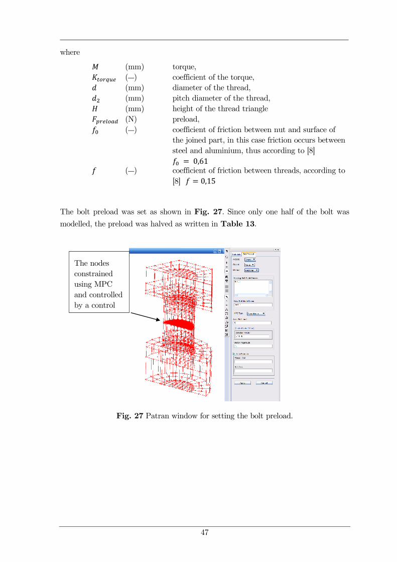
The bolt preload was set as shown in Fig. 27. Since only one half of the bolt was
modelled, the preload was halved as written in Table 13.
Fig. 27 Patran window for setting the bolt preload.
The nodes
constrained
using MPC
and controlled
by a control
node Node
48
Table 13 The loads used in the analyses.
Number of
the step
Load Character Location of ap-
plied load
Step 1 preload P = 1133 N bolt pretension Node 50 660
Step 2 displacement uz = 6 mm main load Node 1
7.7 Setting of the solution
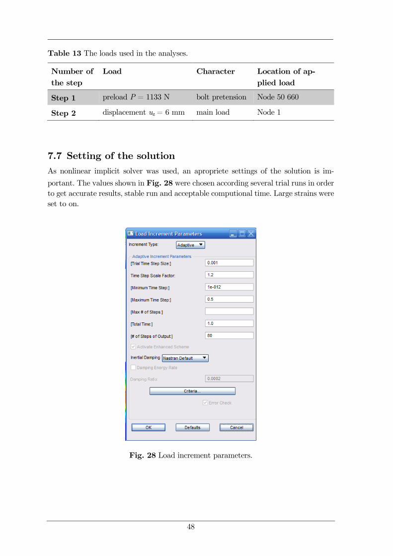
As nonlinear implicit solver was used, an apropriete settings of the solution is im-
portant. The values shown in Fig. 28 were chosen according several trial runs in order
to get accurate results, stable run and acceptable computional time. Large strains were
set to on.
Fig. 28 Load increment parameters.
49
8 Results
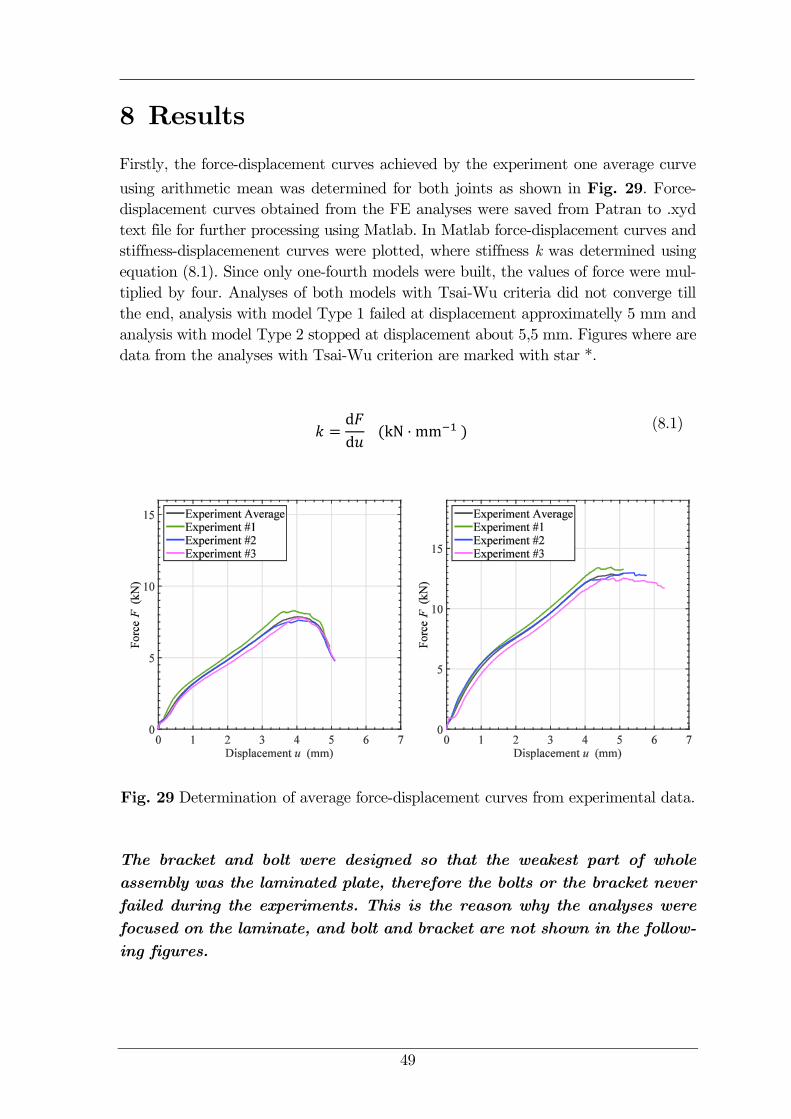
Firstly, the force-displacement curves achieved by the experiment one average curve
using arithmetic mean was determined for both joints as shown in Fig. 29. Force-
displacement curves obtained from the FE analyses were saved from Patran to .xyd
text file for further processing using Matlab. In Matlab force-displacement curves and
stiffness-displacemenent curves were plotted, where stiffness k was determined using
equation (8.1). Since only one-fourth models were built, the values of force were mul-
tiplied by four. Analyses of both models with Tsai-Wu criteria did not converge till
the end, analysis with model Type 1 failed at displacement approximatelly 5 mm and
analysis with model Type 2 stopped at displacement about 5,5 mm. Figures where are
data from the analyses with Tsai-Wu criterion are marked with star *.
𝑘 =
d𝐹
d𝑢 kN ⋅ mm−1
(8.1)
Fig. 29 Determination of average force-displacement curves from experimental data.
The bracket and bolt were designed so that the weakest part of whole
assembly was the laminated plate, therefore the bolts or the bracket never
failed during the experiments. This is the reason why the analyses were
focused on the laminate, and bolt and bracket are not shown in the follow-
ing figures.
50
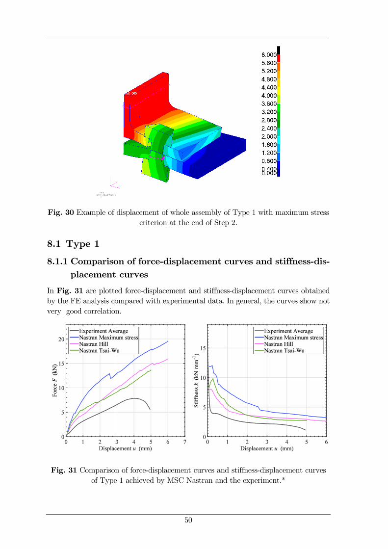
Fig. 30 Example of displacement of whole assembly of Type 1 with maximum stress
criterion at the end of Step 2.
8.1 Type 1
8.1.1 Comparison of force-displacement curves and stiffness-dis-
placement curves
In Fig. 31 are plotted force-displacement and stiffness-displacement curves obtained
by the FE analysis compared with experimental data. In general, the curves show not
very good correlation.
Fig. 31 Comparison of force-displacement curves and stiffness-displacement curves
of Type 1 achieved by MSC Nastran and the experiment.*

51
8.1.2 Displacement and failure index using maximum stress fail-
ure criterion
In the following figures displacement and plots of failure index of Type 1 are shown at
the end of Step 1 and at the end of Step 2 with maximum stress failure criterion, Hill
failure criterion in chapter 8.1.3 and Tsai-Wu criterion in chapter 8.1.4. According to
these figures, small local damage of the laminate occurs from the bolt preload.
Fig. 32 Type 1 with maximum stress criterion. Results at the end of the Step 1: in
the left image is displacement (mm) of the laminated plate in the left image, in the
right image is shown failure index (-) for element.
Fig. 33 Type 1 with maximum stress criterion. Results at the end of the Step 2: in
the left image is displacement (mm) of the laminated plate in the left image, in the
right image is shown failure index (-) for element.
52
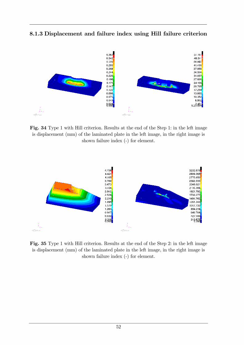
8.1.3 Displacement and failure index using Hill failure criterion
Fig. 34 Type 1 with Hill criterion. Results at the end of the Step 1: in the left image
is displacement (mm) of the laminated plate in the left image, in the right image is
shown failure index (-) for element.
Fig. 35 Type 1 with Hill criterion. Results at the end of the Step 2: in the left image
is displacement (mm) of the laminated plate in the left image, in the right image is
shown failure index (-) for element.
53
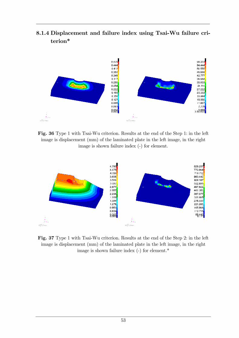
8.1.4 Displacement and failure index using Tsai-Wu failure cri-
terion*
Fig. 36 Type 1 with Tsai-Wu criterion. Results at the end of the Step 1: in the left
image is displacement (mm) of the laminated plate in the left image, in the right
image is shown failure index (-) for element.
Fig. 37 Type 1 with Tsai-Wu criterion. Results at the end of the Step 2: in the left
image is displacement (mm) of the laminated plate in the left image, in the right
image is shown failure index (-) for element.*
54
8.2 Type 2
8.2.1 Comparison of force-displacement curves and stiffness-dis-
placement curves
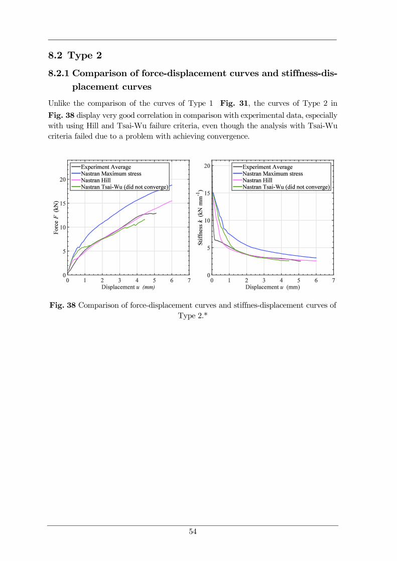
Unlike the comparison of the curves of Type 1 Fig. 31, the curves of Type 2 in
Fig..38 display very good correlation in comparison with experimental data, especially
with using Hill and Tsai-Wu failure criteria, even though the analysis with Tsai-Wu
criteria failed due to a problem with achieving convergence.
Fig..38 Comparison of force-displacement curves and stiffnes-displacement curves of
Type 2.*
55
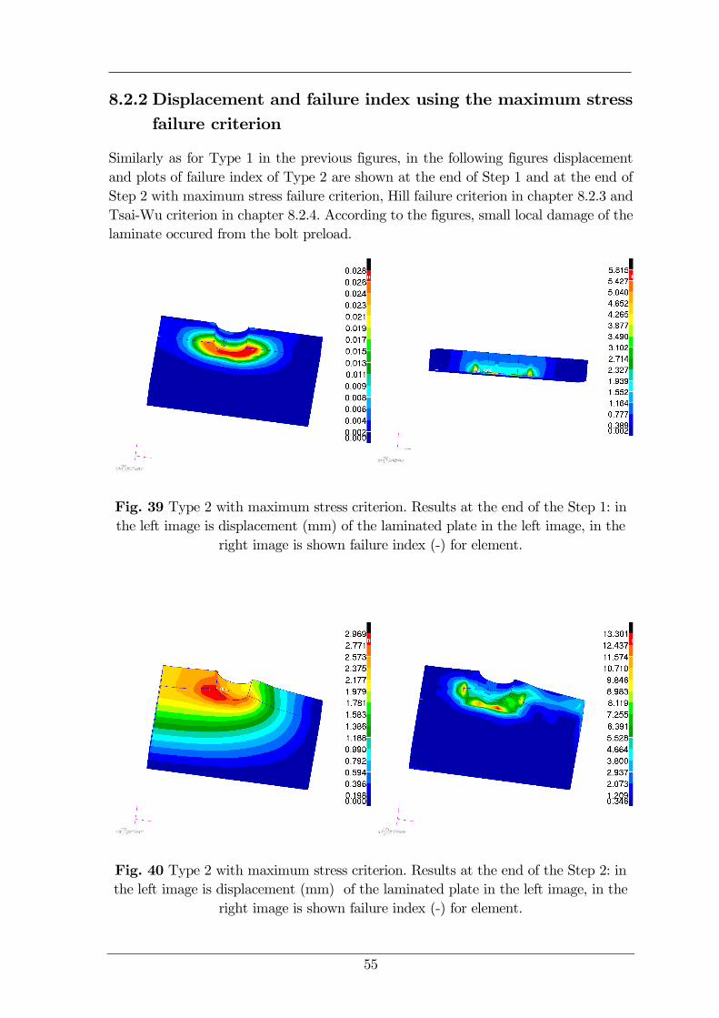
8.2.2 Displacement and failure index using the maximum stress
failure criterion
Similarly as for Type 1 in the previous figures, in the following figures displacement
and plots of failure index of Type 2 are shown at the end of Step 1 and at the end of
Step 2 with maximum stress failure criterion, Hill failure criterion in chapter 8.2.3 and
Tsai-Wu criterion in chapter 8.2.4. According to the figures, small local damage of the
laminate occured from the bolt preload.
Fig. 39 Type 2 with maximum stress criterion. Results at the end of the Step 1: in
the left image is displacement (mm) of the laminated plate in the left image, in the
right image is shown failure index (-) for element.
Fig. 40 Type 2 with maximum stress criterion. Results at the end of the Step 2: in
the left image is displacement (mm) of the laminated plate in the left image, in the
right image is shown failure index (-) for element.
56
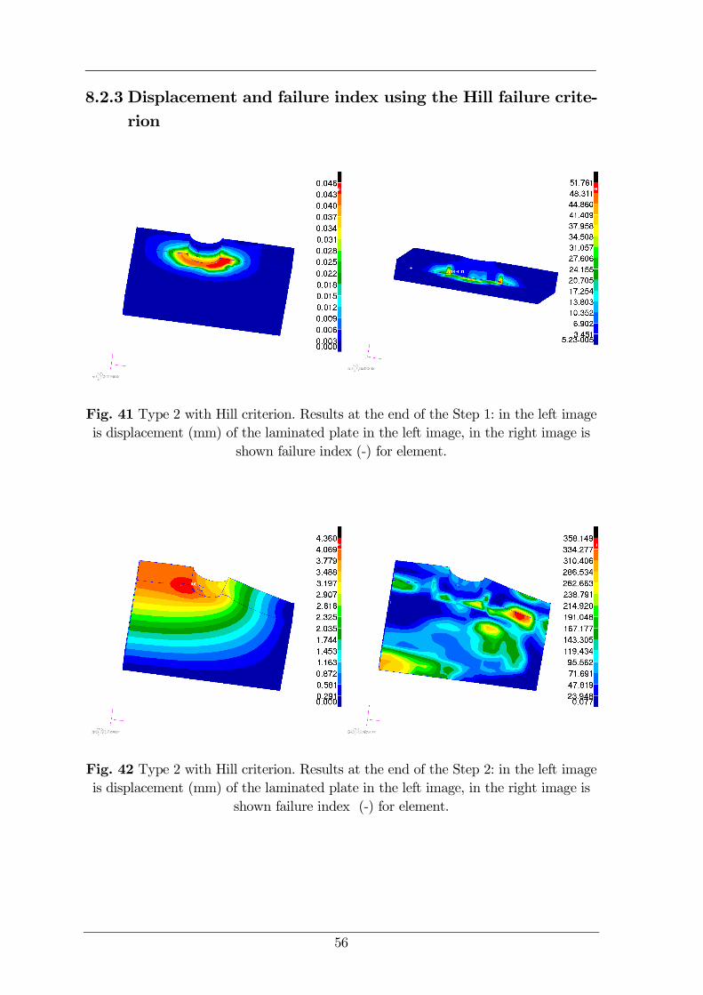
8.2.3 Displacement and failure index using the Hill failure crite-
rion
Fig. 41 Type 2 with Hill criterion. Results at the end of the Step 1: in the left image
is displacement (mm) of the laminated plate in the left image, in the right image is
shown failure index (-) for element.
Fig. 42 Type 2 with Hill criterion. Results at the end of the Step 2: in the left image
is displacement (mm) of the laminated plate in the left image, in the right image is
shown failure index (-) for element.
57
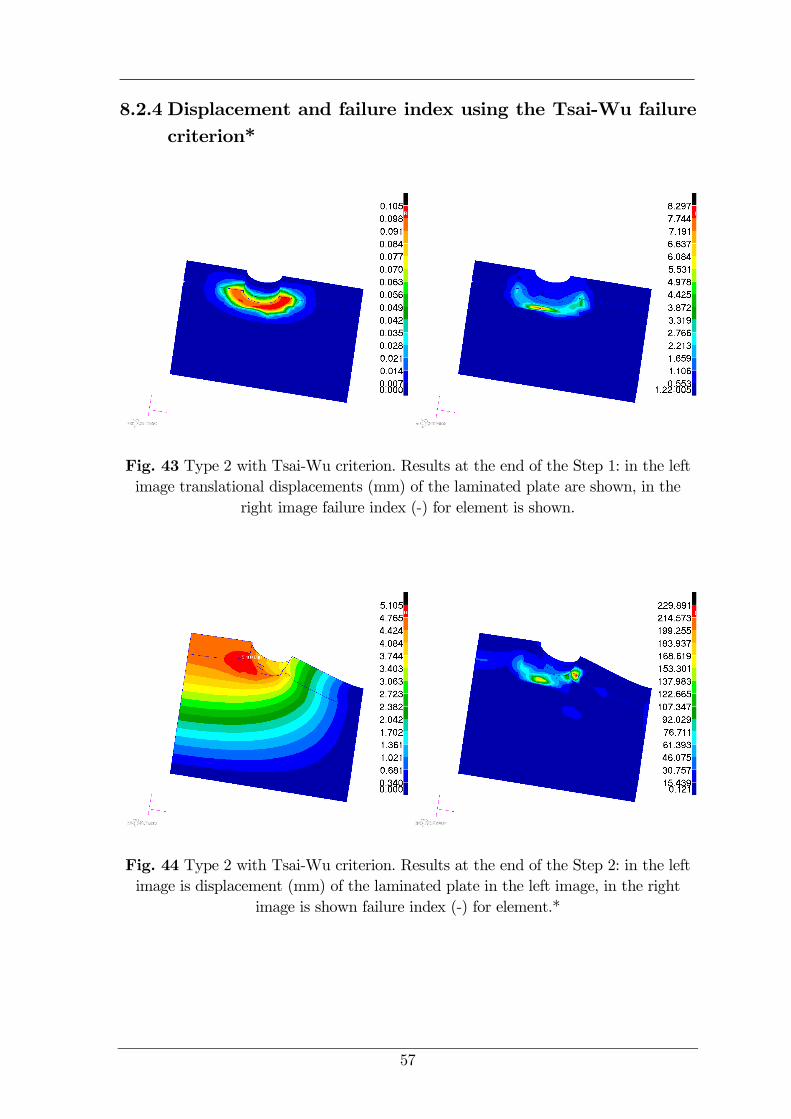
8.2.4 Displacement and failure index using the Tsai-Wu failure
criterion*
Fig. 43 Type 2 with Tsai-Wu criterion. Results at the end of the Step 1: in the left
image translational displacements (mm) of the laminated plate are shown, in the
right image failure index (-) for element is shown.
Fig. 44 Type 2 with Tsai-Wu criterion. Results at the end of the Step 2: in the left
image is displacement (mm) of the laminated plate in the left image, in the right
image is shown failure index (-) for element.*
58
8.3 Comparison of Type 1 and Type 2
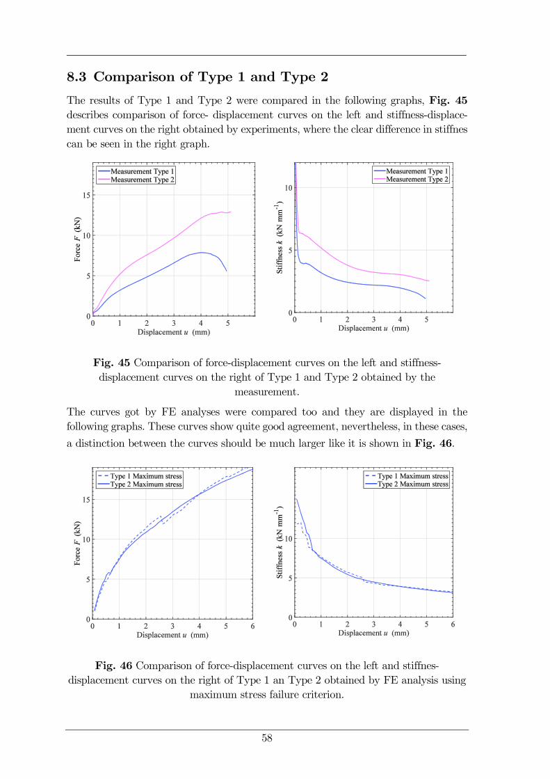
The results of Type 1 and Type 2 were compared in the following graphs, Fig. 45
describes comparison of force- displacement curves on the left and stiffness-displace-
ment curves on the right obtained by experiments, where the clear difference in stiffnes
can be seen in the right graph.
Fig. 45 Comparison of force-displacement curves on the left and stiffness-
displacement curves on the right of Type 1 and Type 2 obtained by the
measurement.
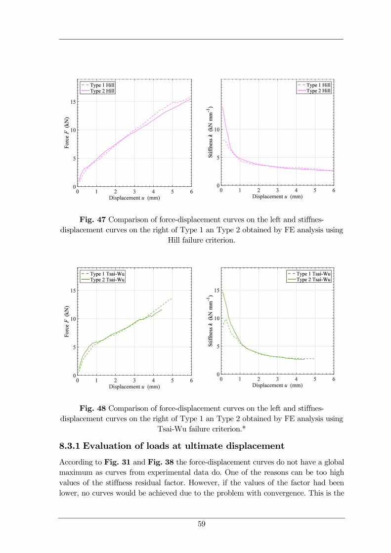
The curves got by FE analyses were compared too and they are displayed in the
following graphs. These curves show quite good agreement, nevertheless, in these cases,
a distinction between the curves should be much larger like it is shown in Fig. 46.
Fig. 46 Comparison of force-displacement curves on the left and stiffnes-
displacement curves on the right of Type 1 an Type 2 obtained by FE analysis using
maximum stress failure criterion.
59
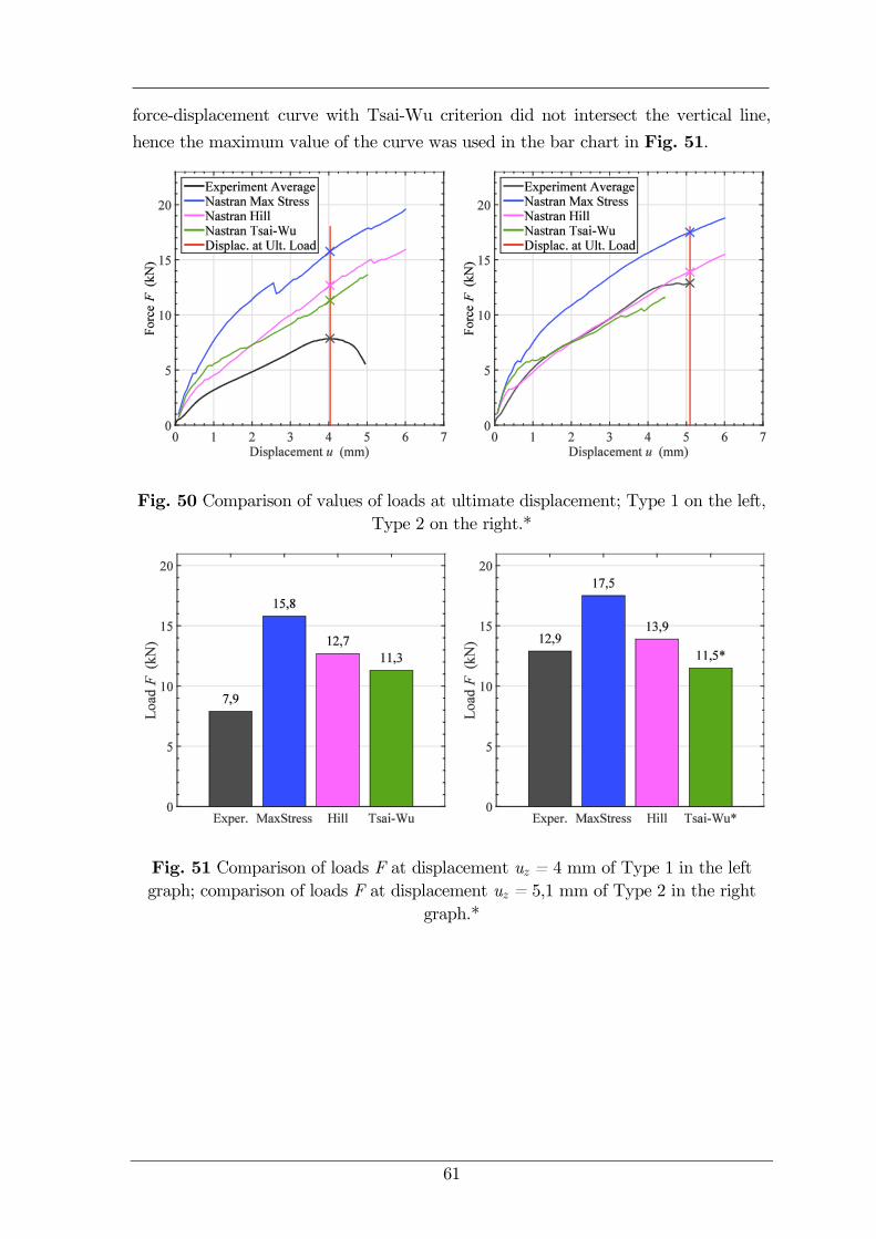
Fig. 47 Comparison of force-displacement curves on the left and stiffnes-
displacement curves on the right of Type 1 an Type 2 obtained by FE analysis using
Hill failure criterion.
Fig. 48 Comparison of force-displacement curves on the left and stiffnes-
displacement curves on the right of Type 1 an Type 2 obtained by FE analysis using
Tsai-Wu failure criterion.*
8.3.1 Evaluation of loads at ultimate displacement
According to Fig. 31 and Fig..38 the force-displacement curves do not have a global
maximum as curves from experimental data do. One of the reasons can be too high
values of the stiffness residual factor. However, if the values of the factor had been
lower, no curves would be achieved due to the problem with convergence. This is the

60
reason why ultimate loads could not be obtained by Nastran solver. Nevertheless,
values of ultimate load were obtained from experimental data, thus for evaluation of
both models a different method was used ― loads were compared at value of ultimate
displacement. The procedure of evaluation of loads at ultimate displacement is written
below:
1. determination of a displacement at the ultimate load from experimental data
as shown in Fig. 49 and plotting a vertical line at the value of the ultimate
displacement in the previous step,
2. an intersection of the vertical line and force-displacement curve will deter-
mine a value of the load at the ultimate displacement as depicted in Fig. 50,
3. an comparison of the values of loads at the ultimate displacement as displa-
yed in Fig. 51.
Fig. 49 Determination of the ultimate load and ultimate displacement of Type 1 on
the left and Type 2 on the right using Matlab from experimental data.
The values of ultimate displacements and loads are written in the Table 14.
Table 14 The values of ultimate displacements and loads obtained
by experiments.
Quantity Type 1 Type 2
ultimate displacement (mm) 4 5,1
ultimate load (kN) 7,9 12,9
Values of load at ultimate displacement obtained by Matlab were compared and re-
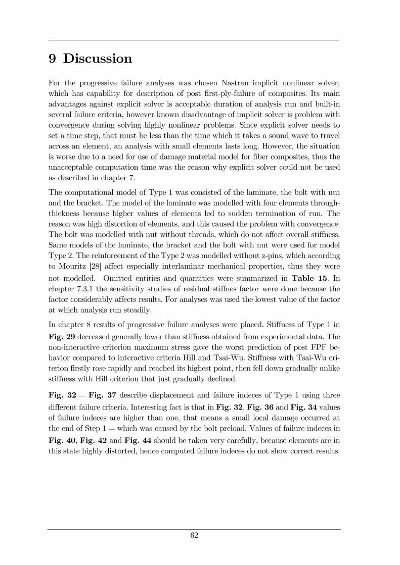
sults are displayed in bar charts in Fig. 51. According to the right graph in Fig. 50,
61
force-displacement curve with Tsai-Wu criterion did not intersect the vertical line,
hence the maximum value of the curve was used in the bar chart in Fig. 51.
Fig. 50 Comparison of values of loads at ultimate displacement; Type 1 on the left,
Type 2 on the right.*
Fig. 51 Comparison of loads F at displacement uz = 4 mm of Type 1 in the left
graph; comparison of loads F at displacement uz = 5,1 mm of Type 2 in the right
graph.*
62
9 Discussion
For the progressive failure analyses was chosen Nastran implicit nonlinear solver,
which has capability for description of post first-ply-failure of composites. Its main
advantages against explicit solver is acceptable duration of analysis run and built-in
several failure criteria, however known disadvantage of implicit solver is problem with
convergence during solving highly nonlinear problems. Since explicit solver needs to
set a time step, that must be less than the time which it takes a sound wave to travel
across an element, an analysis with small elements lasts long. However, the situation
is worse due to a need for use of damage material model for fiber composites, thus the
unacceptable computation time was the reason why explicit solver could not be used
as described in chapter 7.
The computational model of Type 1 was consisted of the laminate, the bolt with nut
and the bracket. The model of the laminate was modelled with four elements through-
thickness because higher values of elements led to sudden termination of run. The
reason was high distortion of elements, and this caused the problem with convergence.
The bolt was modelled with nut without threads, which do not affect overall stiffness.
Same models of the laminate, the bracket and the bolt with nut were used for model
Type 2. The reinforcement of the Type 2 was modelled without z-pins, which according
to Mouritz [28] affect especially interlaminar mechanical properties, thus they were
not modelled. Omitted entities and quantities were summarized in Table 15. In
chapter 7.3.1 the sensitivity studies of residual stiffnes factor were done because the
factor considerably affects results. For analyses was used the lowest value of the factor
at which analysis run steadily.
In chapter 8 results of progressive failure analyses were placed. Stiffness of Type 1 in
Fig. 29 decreased generally lower than stiffness obtained from experimental data. The
non-interactive criterion maximum stress gave the worst prediction of post FPF be-
havior compared to interactive criteria Hill and Tsai-Wu. Stiffness with Tsai-Wu cri-
terion firstly rose rapidly and reached its highest point, then fell down gradually unlike
stiffness with Hill criterion that just gradually declined.
Fig. 32 ― Fig. 37 describe displacement and failure indeces of Type 1 using three
different failure criteria. Interesting fact is that in Fig. 32, Fig. 36 and Fig. 34 values
of failure indeces are higher than one, that means a small local damage occurred at
the end of Step 1 ― which was caused by the bolt preload. Values of failure indeces in
Fig. 40, Fig. 42 and Fig. 44 should be taken very carefully, because elements are in
this state highly distorted, hence computed failure indeces do not show correct results.
63
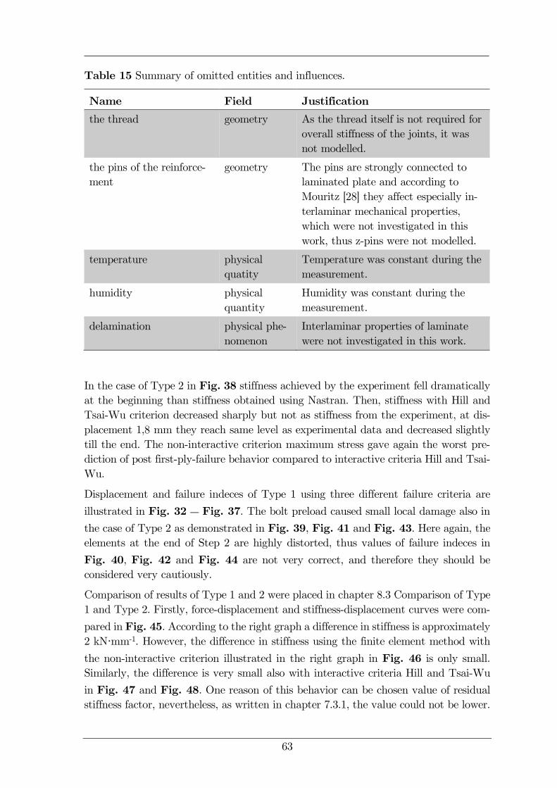
Table 15 Summary of omitted entities and influences.
Name Field Justification
the thread geometry As the thread itself is not required for
overall stiffness of the joints, it was
not modelled.
the pins of the reinforce-
ment
geometry The pins are strongly connected to
laminated plate and according to
Mouritz [28] they affect especially in-
terlaminar mechanical properties,
which were not investigated in this
work, thus z-pins were not modelled.
temperature physical
quatity
Temperature was constant during the
measurement.
humidity physical
quantity
Humidity was constant during the
measurement.
delamination physical phe-
nomenon
Interlaminar properties of laminate
were not investigated in this work.
In the case of Type 2 in Fig..38 stiffness achieved by the experiment fell dramatically
at the beginning than stiffness obtained using Nastran. Then, stiffness with Hill and
Tsai-Wu criterion decreased sharply but not as stiffness from the experiment, at dis-
placement 1,8 mm they reach same level as experimental data and decreased slightly
till the end. The non-interactive criterion maximum stress gave again the worst pre-
diction of post first-ply-failure behavior compared to interactive criteria Hill and Tsai-
Wu.
Displacement and failure indeces of Type 1 using three different failure criteria are
illustrated in Fig. 32 ― Fig. 37. The bolt preload caused small local damage also in
the case of Type 2 as demonstrated in Fig. 39, Fig. 41 and Fig. 43. Here again, the
elements at the end of Step 2 are highly distorted, thus values of failure indeces in
Fig. 40, Fig. 42 and Fig. 44 are not very correct, and therefore they should be
considered very cautiously.
Comparison of results of Type 1 and 2 were placed in chapter 8.3 Comparison of Type
1 and Type 2. Firstly, force-displacement and stiffness-displacement curves were com-
pared in Fig. 45. According to the right graph a difference in stiffness is approximately
2 kN∙mm-1. However, the difference in stiffness using the finite element method with
the non-interactive criterion illustrated in the right graph in Fig. 46 is only small.
Similarly, the difference is very small also with interactive criteria Hill and Tsai-Wu
in Fig. 47 and Fig. 48. One reason of this behavior can be chosen value of residual
stiffness factor, nevertheless, as written in chapter 7.3.1, the value could not be lower.
64
According to the text in chapter 8.3.1, the force-displacement curves do not have a
global maximum as curves from the experiment do, therefore ultimate loads were ob-
tained only from experimental data and could not be compared with results of finite
element analyses. However, loads at ultimate displacement were compared instead in
Fig. 50 and Fig. 51, where in respective graphs a difference between used failure
criteria is nicely illustrated, which can help to choose a right criterion for evaluation
of composite structure.
65
10 Conclusion
The main aim of this thesis was investigation of post first-ply-failure of metal-to-com-
posite joints with emphasis on laminate using three different failure criteria by the
finite element method. One non-interactive criterion the maximum stress and two
interactive criteria Hill and Tsai-Wu were used for studying behavior of composite
material in the work.
In the introductory part of the thesis were described the analyzed problems and the
research study of progressive failure analysis of bolted joints, mechanics of composite
materials and the finite element method. Computional models were depicted in the
chapter 7, where important sensitivity studies of residual stiffness factor were described
too and in the chapter 8 were placed results of the performed analyses.
According these results the following concluding statements can be claimed:
In general, interactive criteria Hill and Tsai-Wu failure criteria gave similar
prediction of post first-ply-failure behavior.
Non-interactive criterion gave considerably higher values of force and stiffness
than interactive criteria and its prediction of post first-ply-failure behavior is
the worst compared to experimental data, thus interactive criteria are more
apropriate for prediction of post FPF behavior of composites.
Very good agreement of the results of FE analyses and the experiment had
force-displacement curves of Type 2, especially with the Hill and Tsai-Wu cri-
teria; the agreement in the case of the Type 1 is less satisfying. In general, the
agreement is better in the case of Type 2 than in the case of Type 1.
All the results are strongly dependant on the value of residual stiffness factor,
thus accuracy can be increased, but too low values of the factor can result in
problems with obtaining the convergence. Since the problems are caused mostly
by extremely large distorsion of the elements, the solution of the problems can
be a use of a different nonlinear solver, which allow the element death technique
and remeshing. As Nastran Implicit Nonlinear SOL 400 does not allow such
advanced methods, therefore these methods could not be used for the analyses.
The most used solvers, which allow the element death technique and remeshing
and have capability for the progressive failure analysis of composites, are MSC
Marc and Abaqus. Explicit solver can be used too, but duration of analysis can
take enormous time.
If computional models are firstly harmonized according to experimental data,
then the progressive failure analyses will give good prediction of post first-ply-
failure behavior of material.
66
References
Books
[1] JANÍČEK, Přemysl. Systémova metodologie: Brána do řešení problému. 1st
ed. Brno: CERM Academické vydavatelství, 2014. ISBN 978-80-7204-887-8.
[2] VRBKA, Jan. Mechanika kompozitů. In: Insitute of solid mechanics, mech-
atronics and biomechanics FME BUT [online], 2008. [cit. 2015-10-21] Avai-
lable online on: https://www.vutbr.cz/www_base/priloha.php?dpid=83340
[3] DANIEL, Isaac. M. and Ori ISHAI. Engineeering mechanics of composite
materials. 2nd ed. New York: Oxford University Press, 2006.ISBN 978-0-19-
515097-1
[4] PETRUŠKA, Jindřich. MKP v inženýrských výpočtech. Brno university of
technology FME: Institute of solid mechanics, mechatronics and biome-
chanics [online]. 2011. [cit. 2015-04-10]. Available online on:
http://www.umt.fme.vutbr.cz/img/fckeditor/file/opory/RIV/MKP2011.pdf
[5] MALVERN, Lawrence E. Introduction to the mechanics of a continuous
medium. New Jersey: Prentice-Hall, 1969. ISBN 978-0134876030
[6] JONES, Robert Millard. Mechanics of composite materials. 2nd ed. New
York: Hemisphere Publishing Corporation, 1999. ISBN 1-56032-712-X
[7] BAKER, A., S. DUTTON and D. KELLY. Composite Materials for Air-
craft Structures. 2nd ed. Reston: American Institute of Aeronautics and As-
tronautics , 2004. ISBN 1-56347-540-5
[8] SHIGLEY, J.E., C.R. MISCHKE and R.G BUDYNAS. Kontruování stro-
jních součástí. Brno: VUTIUM Akademické vydavatelství, 2010. ISBN 978-
80-214-2629-0
[9] JANÍČEK, P., J. MAREK a kol. Expertní inženýrství v systémovém pojetí.
Praha: Grada Publishing, 2013. ISBN 978-80-247-4127-7
[10] ZIENKIEWICZ, Olgierd Cecil. The finite element method. 5th ed., Volume
1: The Basis. Oxford: Butterworth-Heinemann, 2000. ISBN 0-7506-5049-4
[11] LEINVEBER, Jan. and Pavel VÁVRA. Strojnické tabulky. 2nd ed. Úvaly:
Albra, 2005. ISBN 80-7361-011-6
[12] NOVÁK, Kamil. Analýza zbytkových napětí ve stěně tepny. Brno, 2013.
Master’s thesis. Brno university of technology, Faculty of mechanical engi-
neering, Institute of mechanics, mechatronics and biomechanics.
67
[13] MSC Software. MSC Nastran 2014 Nonlinear User’s Guide SOL 400: MSC
Software, ® 2014.
[14] MSC Software. MSC Patran User’s Guide: MSC Software, ® 2014.
Scientific reasearch papers
[15] HART-SMITH, L. J. Design and empirical analysis of bolted or riveted
joints. Joining Fibre-Reinforced Plastics. 1987, pp. 227-269.
[16] TSAI, Stephen W. A general theory of strength for anisotropic materials.
Journal of composite materials. 1971, vol.5 : pp. 58-80. Available online on:
http://www.dtic.mil/cgi-bin/GetTRDoc?AD=ADA306350
[17] ADAM, L., C. BOUVET, B. CASTANIÉ, A. DAIDIÉ and E.
BONHOMME. Discrete ply model of circular pull-through test of fasteners
in laminates. Composite Structures. 2012, vol. 94: pp. 3082-3091. Available
online on:
http://www.sciencedirect.com/science/article/pii/S0263822312002176
[18] HEIMBS, S., S. SCHMEER, J. BLAUROCK and S. STEEGER. Static and
dynamic failure behaviour of bolted joints in carbon fibre composites. Com-
posites: Part A Applied Science and Manufacturing. 2013, vol 47: pp. 91-
101. Available online on:
http://www.sciencedirect.com/science/article/pii/S1359835X12003697
[19] KABCHE, J.P., V. CACCESE, K.A. BERUBE and R. BRAGG. Experi-
mental characterization of hybrid composite-to-metal bolted joints under
flexural loading. Composites Part B. 2007, vol. 38: pp. 66-78. Available
online on:
http://www.sciencedirect.com/science/article/pii/S135983680600059X
[20] KELLY, Gordon and Stefan HALLSTROM. Strength and failure mecha-
nisms of composite laminates subject to localised transverse loading. Com-
posite structures. 2005, vol. 69: pp. 301-314. Available online on:
http://www.sciencedirect.com/science/article/pii/S0263822304002375
[21] CATALANOTTI, G., P.P CAMANHO, P. GHYS and A.T MARQUES.
Experimental and numerical study of fastener pull-through failure in GFRP
laminates. Composite structures. 2011, vol. 94: pp. 239-245. Available
online on:
http://www.sciencedirect.com/science/article/pii/S0263822311002418
68
[22] ELDER, D.J., A.H. VERDAASDONK and R.S THOMSON. Fastener pull-
through in a carbon fibre epoxy composite joint. Composite structures.
2008, vol. 86: pp. 291-298. Available online on:
http://www.sciencedirect.com/science/article/pii/S0263822308000925
[23] STOCCHI, C., P. ROBINSON and S.T PINHO. A detailed finite element
investigation of composite bolted joints with countersunk fasteners. Compo-
sites Part A: Applied Science and Manufacturing. 2013, vol. 52: pp. 143-
150. Available online on:
http://www.sciencedirect.com/science/article/pii/S1359835X1200303X
[24] CAMANHO, Pedro P. and F.L. MATTHEWS. Stress analysis and
strength prediction of mechanically fastened joints in FRP. Composite part
A: Applied Science and manufacturing. 1997, vol. 28: pp. 529-547. Availa-
ble online on:
http://www.sciencedirect.com/science/article/pii/S1359835X97000043
[25] MCCARTHY, C. T., M.A. MCCARTHY and V.P. LAWLOR. Progressive
damage analysis of multi-bolt composite joints with variable bolt-hole clear-
ance. Composites Part B Engineering. 2005, vol. 36: pp. 290-305.
Available online on:
http://www.sciencedirect.com/science/article/pii/S1359836804001404
[26] WANG, Z., S. ZHOU, J. ZHANG and L. ZHOU. Progressive failure analy-
sis of bolted single-lap composite joint based on extended finite element
method. Materials & Design. 2011, vol. 37: pp. 582-588. Available online
on: http://www.sciencedirect.com/science/article/pii/S0261306911006054
[27] HÜHNE, C., A. K. ZERBST, G. KUHLMAN and R. ROLFES. Progres-
sive damage analysis of composite bolted joints with liquid shim layers
usint constant and continuous degradation models. Composite Structures.
2010, vol. 92: pp. 189-200. Available online on:
http://www.sciencedirect.com/science/article/pii/S0263822309002049
[28] MOURITZ, Adrian P. Review of z-pinned composite laminates. Compo-
sites: Part A. 2007, vol. 38: pp. 2383-2397. Available online on:
http://www.sciencedirect.com/science/article/pii/S1359835X07001479
69
Internet sources
[29] BURŠA, Jiří. Constitutive relations of materials (lectures 2015). In: Insti-
tute of solid mechanics, mechatronics and biomechanics FME BUT
[online], 2015. [cit. 2015-11-18] Available online on:
http://www.umt.fme.vutbr.cz/~jbursa/Konstitutivni%20modely.7z
[30] PETRUŠKA, Jindřich. Nonlinear problems of mechanics in FEM. In: In-
stitute of solid mechanics, mechatronics and biomechanics FME BUT
[online], 2015. [cit. 2015-04-11] Available online on:
http://www.umt-old.fme.vutbr.cz/%7Ejpetruska/nelin-
earni_mechanika/RNK.zip
[31] MSC Software. Composites Technology Day - Section 1 Introduction to
Composites: MSC Software, ® 2012. [online] [cit. 2016-03-05]
Available online on:
http://pages.mscsoftware.com/rs/mscsoftware/images/sec1_in-
tro_to_composites_021712.pdf
[32] FLUGKERI2: A350XWB-Demo.jpg. In: https://commons.wiki-
media.org/wiki [online]. 22 July 2015 [cit. 2016-01–02]. Available on:
https://upload.wikimedia.org/wikipedia/commons/b/b1/A350XWB-
Demo.jpg
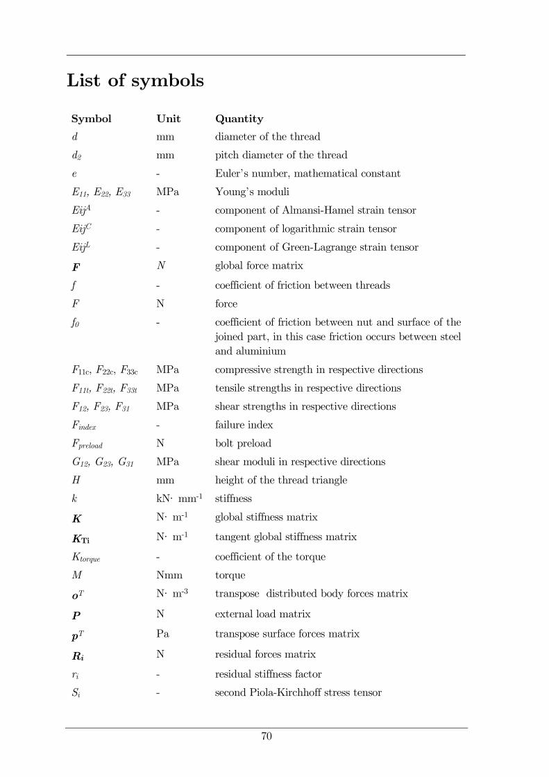
70
List of symbols
Symbol Unit Quantity
d mm diameter of the thread
d2 mm pitch diameter of the thread
e - Euler’s number, mathematical constant
E11, E22, E33 MPa Young’s moduli
EijA - component of Almansi-Hamel strain tensor
EijC - component of logarithmic strain tensor
EijL - component of Green-Lagrange strain tensor
F N global force matrix
f - coefficient of friction between threads
F N force
f0 - coefficient of friction between nut and surface of the
joined part, in this case friction occurs between steel
and aluminium
F11c, F22c, F33c MPa compressive strength in respective directions
F11t, F22t, F33t MPa tensile strengths in respective directions
F12, F23, F31 MPa shear strengths in respective directions
Findex - failure index
Fpreload N bolt preload
G12, G23, G31 MPa shear moduli in respective directions
H mm height of the thread triangle
k kN∙ mm-1 stiffness
K N∙ m-1 global stiffness matrix
KTi N∙ m-1 tangent global stiffness matrix
Ktorque - coefficient of the torque
M Nmm torque
oT N∙ m-3 transpose distributed body forces matrix
P N external load matrix
pT Pa transpose surface forces matrix
Ri N residual forces matrix
ri - residual stiffness factor
Si - second Piola-Kirchhoff stress tensor
71
U m global displacement matrix
ui m displacement matrix
UT m transpose displacement matrix
uT m transpose displacement matrix
uz mm displacement in direction z
W J strain energy
X1, X2, X3 m coordinates of the particle in the Lagrangian descrip-
tion
x1, x2, x3 m coordinates of the particle in the Eulerian descrition
δF, δu convergence criteria
Δui m displacement increment
εT - transpose strain matrix
λi - stretch ratio
ν12, ν23, ν31 - Poisson’s ratios in respective directions
Π J total potential energy
π - mathematical constant
σi Pa component of the first Piola-Kirchhoff stress tensor
σT Pa transpose stress matrix
σyp Pa yield point, yield stress
τi Pa component of Cauchy stress tensor

72
List of abreviations and names of software
FEM finite element method
PFA progressive failure analysis
FPF first-ply-failure
CFRP carbon fiber reinforced polymer
GFRP glass fiber reinforced polymer
MSC Marc implicit nonlinear finite element solver
Abaqus implicit and explicit nonlinear finite element solver
Ansys implicit nonlinear finite element solver
MSC Nastran SOL 400 implicit nonlinear finite element solver
MSC Patran preprocessor and postprocessor for preparation finite ele-
ment models and evaluating results
73
List of figures
Fig. 1 Airbus A350XWB has fuselage and wings made of CFRP. [32] ................................ 12
Fig. 2 Schematics of the system of important quantities.[12] ................................................ 15
Fig. 3 Technical drawing of the joint Type 1. ....................................................................... 16
Fig. 4 Technical drawing of the joint Type 2. ....................................................................... 17
Fig. 5 Schematic illustration of main failure modes in mechanical joints in composites.[15] 17
Fig. 6 Top side of laminated plates of the joints after the measurement; on the left Type 1,
on the right Type 2. Published with permission of Institute of aerospace engineering of Brno
university of technology. .......................................................................................................... 18
Fig. 7 Bottom side of laminated plates of the joints after the measurement; on the left Type
1, on the right Type 2. Published with permission of Institute of aerospace engineering of Brno
university of technology. .......................................................................................................... 18
Fig. 8 Comparison of behaviour of isotropic, orthotropic and anisotropic material. [6] ........ 21
Fig. 9 The base othotropic cooordinate system.[2]................................................................. 22
Fig. 10 Loaded element of orthotropic material in principal orthotropic directions. [2] ....... 23
Fig. 11 Failure envelope for unidirectional lamina under biaxial normal loading (maximum
stress theory). [3] ...................................................................................................................... 24
Fig. 12 Failure envelopes for unidirectional E-glass/epoxy lamina under biaxial loading with
different levels of shear stress (Tsai-Wu criterion). [3] ............................................................ 27
Fig. 13 Graphical representation of Newton-Raphson iterative solution. [30] ...................... 32
Fig. 14 Technical drawing of the joint Type1 clamped using the clamps for measurement,
with red dashed lines demarked one fourth of joint, which was used for the computional models;
same claping systém was used for testing the joint Type 2. ................................................... 36
Fig. 15 Geometry of the computional model Type 1. ............................................................ 37
Fig. 16 Geometry of the computional model Type 2. ............................................................ 37
Fig. 17 Description of refined locations, refined locations in the red ellipses. ....................... 38
Fig. 18 Type 1 – meshed assembly. ....................................................................................... 39
Fig. 19 Type 2 - meshed assembly, isometric view on the left, bottom view on the right. .. 39
Fig. 20 Patran window for input strength limits, residual stiffness factor is in the red box. 42
Fig. 21 Results of the sensitivity study of residual stiffness factor ri using the computional
model Type 2. .......................................................................................................................... 42
Fig. 22 Boundary conditions. ................................................................................................. 43
Fig. 23 Description of used contact bodies of Type 1. ........................................................... 43
74
Fig. 24 Description of used contact bodies of Type 2. ........................................................... 44
Fig. 25 Locations of weak spring for stabilization of the bolt inside the hole. ...................... 45
Fig. 26 Nastran RBE2 element. ............................................................................................. 46
Fig. 27 Patran window for setting the bolt preload. .............................................................. 47
Fig. 28 Load increment parameters. ...................................................................................... 48
Fig. 29 Determination of average force-displacement curves from experimental data. ......... 49
Fig. 30 Example of displacement of whole assembly of Type 1 with maximum stress criterion
at the end of Step 2.................................................................................................................. 50
Fig. 31 Comparison of force-displacement curves and stiffness-displacement curves of Type 1
achieved by MSC Nastran and the experiment.* .................................................................... 50
Fig. 32 Type 1 with maximum stress criterion. Results at the end of the Step 1: in the left
image is displacement (mm) of the laminated plate in the left image, in the right image is
shown failure index (-) for element. ......................................................................................... 51
Fig. 33 Type 1 with maximum stress criterion. Results at the end of the Step 2: in the left
image is displacement (mm) of the laminated plate in the left image, in the right image is
shown failure index (-) for element. ......................................................................................... 51
Fig. 34 Type 1 with Hill criterion. Results at the end of the Step 1: in the left image is
displacement (mm) of the laminated plate in the left image, in the right image is shown failure
index (-) for element. ............................................................................................................... 52
Fig. 35 Type 1 with Hill criterion. Results at the end of the Step 2: in the left image is
displacement (mm) of the laminated plate in the left image, in the right image is shown failure
index (-) for element. ............................................................................................................... 52
Fig. 36 Type 1 with Tsai-Wu criterion. Results at the end of the Step 1: in the left image is
displacement (mm) of the laminated plate in the left image, in the right image is shown failure
index (-) for element. ............................................................................................................... 53
Fig. 37 Type 1 with Tsai-Wu criterion. Results at the end of the Step 2: in the left image is
displacement (mm) of the laminated plate in the left image, in the right image is shown failure
index (-) for element.* .............................................................................................................. 53
Fig..38 Comparison of force-displacement curves and stiffnes-displacement curves of Type 2.*
.................................................................................................................................................. 54
Fig. 39 Type 2 with maximum stress criterion. Results at the end of the Step 1: in the left
image is displacement (mm) of the laminated plate in the left image, in the right image is
shown failure index (-) for element. ......................................................................................... 55
Fig. 40 Type 2 with maximum stress criterion. Results at the end of the Step 2: in the left
image is displacement (mm) of the laminated plate in the left image, in the right image is
shown failure index (-) for element. ......................................................................................... 55
75
Fig. 41 Type 2 with Hill criterion. Results at the end of the Step 1: in the left image is
displacement (mm) of the laminated plate in the left image, in the right image is shown failure
index (-) for element. ............................................................................................................... 56
Fig. 42 Type 2 with Hill criterion. Results at the end of the Step 2: in the left image is
displacement (mm) of the laminated plate in the left image, in the right image is shown failure
index (-) for element. .............................................................................................................. 56
Fig. 43 Type 2 with Tsai-Wu criterion. Results at the end of the Step 1: in the left image
translational displacements (mm) of the laminated plate are shown, in the right image failure
index (-) for element is shown. ................................................................................................ 57
Fig. 44 Type 2 with Tsai-Wu criterion. Results at the end of the Step 2: in the left image is
displacement (mm) of the laminated plate in the left image, in the right image is shown failure
index (-) for element.* ............................................................................................................. 57
Fig. 45 Comparison of force-displacement curves on the left and stiffness-displacement curves
on the right of Type 1 and Type 2 obtained by the measurement. ........................................ 58
Fig. 46 Comparison of force-displacement curves on the left and stiffnes-displacement curves
on the right of Type 1 an Type 2 obtained by FE analysis using maximum stress failure
criterion. ................................................................................................................................... 58
Fig. 47 Comparison of force-displacement curves on the left and stiffnes-displacement curves
on the right of Type 1 an Type 2 obtained by FE analysis using Hill failure criterion. ........ 59
Fig. 48 Comparison of force-displacement curves on the left and stiffnes-displacement curves
on the right of Type 1 an Type 2 obtained by FE analysis using Tsai-Wu failure criterion.*
................................................................................................................................................. 59
Fig. 49 Determination of the ultimate load and ultimate displacement of Type 1 on the left
and Type 2 on the right using Matlab from experimental data. ............................................ 60
Fig. 50 Comparison of values of loads at ultimate displacement; Type 1 on the left, Type 2
on the right.* ........................................................................................................................... 61
Fig. 51 Comparison of loads F at displacement uz = 4 mm of Type 1 in the left graph;
comparison of loads F at displacement uz = 5,1 mm of Type 2 in the right graph.* ............. 61
76
List of tables
Table 1 Comparison of failure index and strength ratio........................................................ 28
Table 2 Comparison of capabilities of implicit and explicit solvers. ..................................... 35
Table 3 Mesh sensitivity study. ............................................................................................. 38
Table 4 Material properties of one lamina of glass fiber reinforced polymer. ....................... 40
Table 5 Stacking sequence. .................................................................................................... 40
Table 6 Material properties of aluminium alloy D16. ............................................................ 41
Table 7 Materials properties for steel of the bolt. ................................................................. 41
Table 8 Material properties for steel of the reinforcement. ................................................... 41
Table 9 List of contact used in model Type 1 ....................................................................... 44
Table 10 List of contact used in model Type 2. .................................................................... 44
Table 11 Geometrical properties of touched contact. ............................................................ 44
Table 12 Physical properties of touched contact. .................................................................. 45
Table 13 The loads used in the analyses. .............................................................................. 48
Table 14 The values of ultimate displacements and loads obtained ..................................... 60
Table 15 Summary of omitted entities and influences. ......................................................... 63