by

Madhu Kaundal

Contributors: Mihir Kumar Dash, Jithendra Raju N.

Indian Institute of Technology Kharagpur, India

April 30, 2021

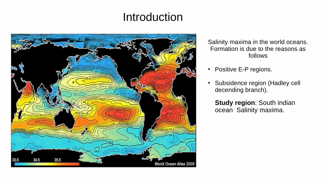
Introduction

Salinity maxima in the world oceans. Formation is due to the reasons as

follows

● Positive E-P regions.

● Subsidence region (Hadley cell decending branch).

Study region: South indian ocean Salinity maxima.

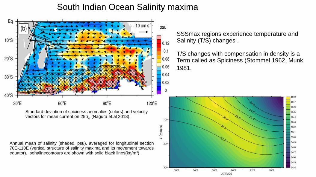
Standard deviation of spiciness anomalies (colors) and velocity vectors for mean current on 25σ

Θ (Nagura et.al 2018).).

Annual mean of salinity (shaded, psu), averaged for longitudinal section 70E-110E (vertical structure of salinity maxima and its movement towards equator). Isohalinecontours are shown with solid black lines(kg/m3) .

South Indian Ocean Salinity maxima

SSSmax regions experience temperature andSalinity (T/S) changes .

T/S changes with compensation in density is aTerm called as Spiciness (Stommel 1962, Munk 198).1.

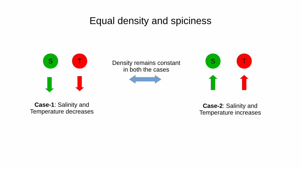
Equal density and spiciness

S T S TDensity remains constant in both the cases

Case-1: Salinity and Temperature decreases

Case-2: Salinity and Temperature increases

Spiciness processes

Subsurface T/S changes can be formed locally through two main process.

● Suduction process

● Injection process

Subduction: occurs where an isopycnal outcrops and sea surface

spiciness (T/S changes) anomalies are found and then they subduct in to

the main thermocline along the isopycnal surface.

Injection: When isopycnal is not exposed to the surface but large

destabilizing salinity gradients are present in conjuction with the weak

stratification( weak temperature gradient) and thus due to convective mixing

at the base of mixed layer saline water is injected into the main thermocline.

Background Basis

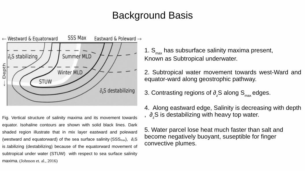
Fig. Vertical structure of salinity maxima and its movement towards

equator. Isohaline contours are shown with solid black lines. Dark

shaded region illustrate that in mix layer eastward and poleward

(westward and equatorward) of the sea surface salinity (SSSmax), ∂zS

is stabilizing (destabilizing) because of the equatorward movement of

subtropical under water (STUW) with respect to sea surface salinity

maxima. (Johnson et. al., 2016)

1. Smax

has subsurface salinity maxima present, Known as Subtropical underwater.

2. Subtropical water movement towards west-Ward and equator-ward along geostrophic pathway.

3. Contrasting regions of ∂zS along S

max edges.

4. Along eastward edge, Salinity is decreasing with depth , ∂

zS is destabilizing with heavy top water.

5. Water parcel lose heat much faster than salt and become negatively buoyant, suseptible for finger convective plumes.

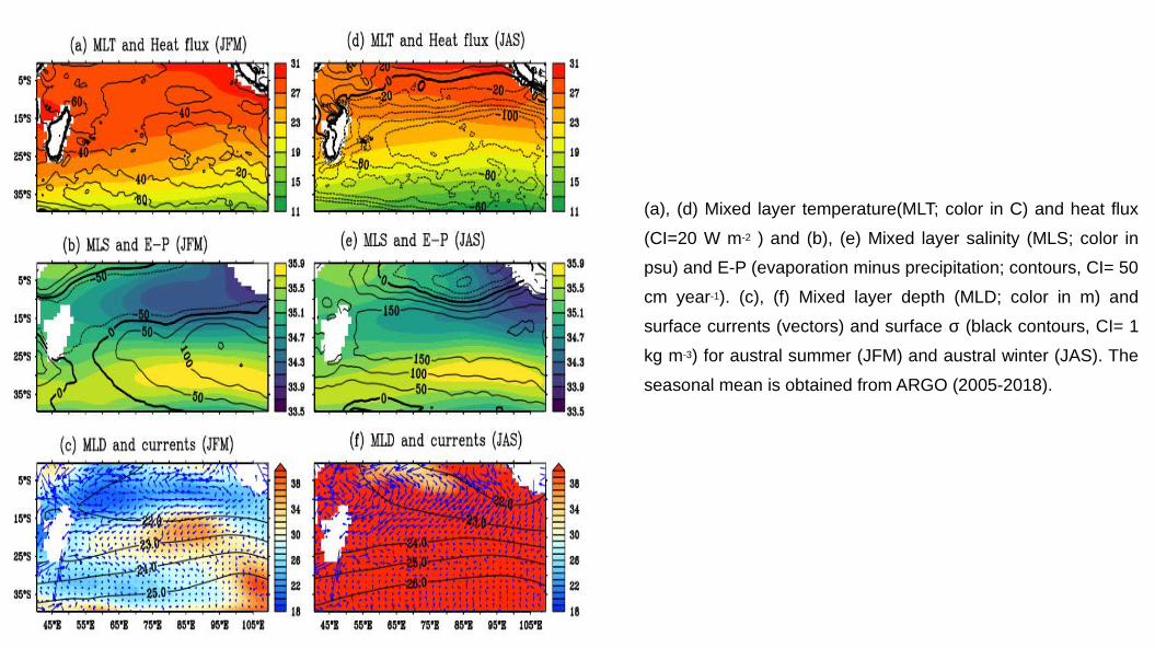
(a), (d) Mixed layer temperature(MLT; color in C) and heat flux

(CI=20 W m-2 ) and (b), (e) Mixed layer salinity (MLS; color in

psu) and E-P (evaporation minus precipitation; contours, CI= 50

cm year-1). (c), (f) Mixed layer depth (MLD; color in m) and

surface currents (vectors) and surface σ (black contours, CI= 1

kg m-3) for austral summer (JFM) and austral winter (JAS). The

seasonal mean is obtained from ARGO (2005-2018).).

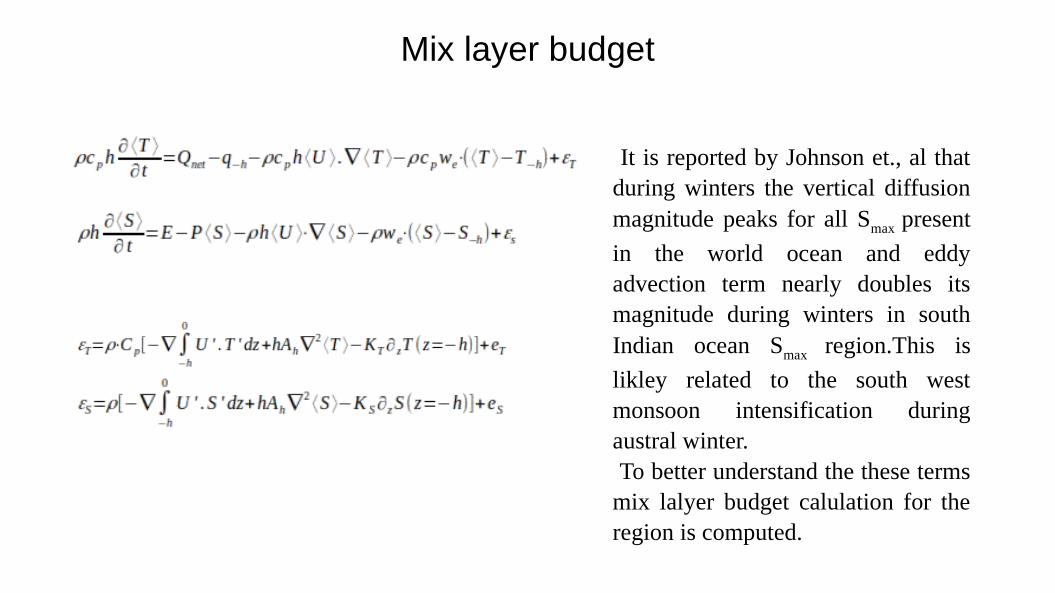
Mix layer budget

It is reported by Johnson et., al that during winters the vertical diffusion magnitude peaks for all Smax present

in the world ocean and eddy advection term nearly doubles its magnitude during winters in south Indian ocean Smax region.This is

likley related to the south west monsoon intensification during austral winter. To better understand the these terms mix lalyer budget calulation for the region is computed.

Data validation

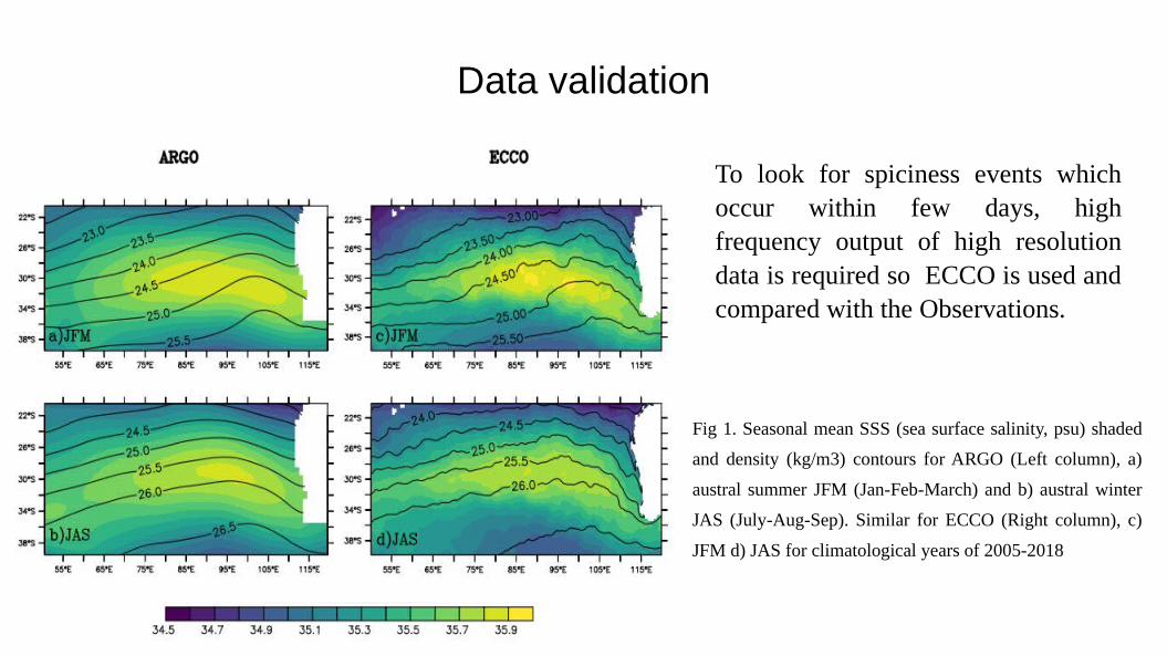
Fig 1. Seasonal mean SSS (sea surface salinity, psu) shaded

and density (kg/m3) contours for ARGO (Left column), a)

austral summer JFM (Jan-Feb-March) and b) austral winter

JAS (July-Aug-Sep). Similar for ECCO (Right column), c)

JFM d) JAS for climatological years of 2005-2018

To look for spiciness events which occur within few days, high frequency output of high resolution data is required so ECCO is used and compared with the Observations.

North box

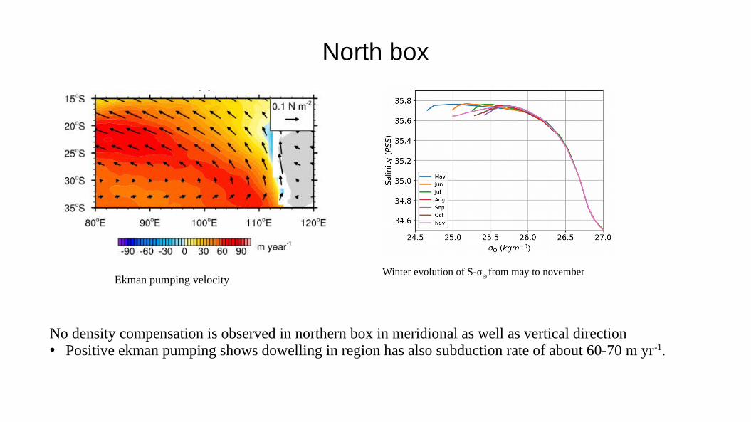
Ekman pumping velocityWinter evolution of S-σ

Θ from may to november

No density compensation is observed in northern box in meridional as well as vertical direction● Positive ekman pumping shows dowelling in region has also subduction rate of about 60-70 m yr-1.

Turner angle

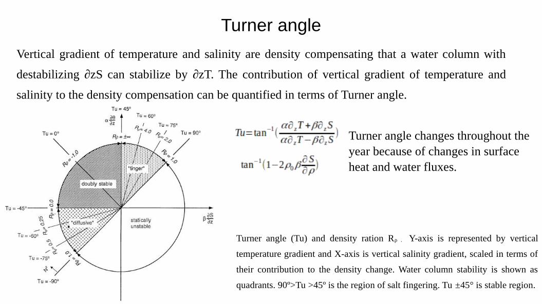
Turner angle (Tu) and density ration Rρ . Y-axis is represented by vertical

temperature gradient and X-axis is vertical salinity gradient, scaled in terms of

their contribution to the density change. Water column stability is shown as

quadrants. 90º>Tu >45º is the region of salt fingering. Tu ±45° is stable region.

Vertical gradient of temperature and salinity are density compensating that a water column with

destabilizing ∂zS can stabilize by ∂zT. The contribution of vertical gradient of temperature and

salinity to the density compensation can be quantified in terms of Turner angle.

Turner angle changes throughout the year because of changes in surface heat and water fluxes.

South box

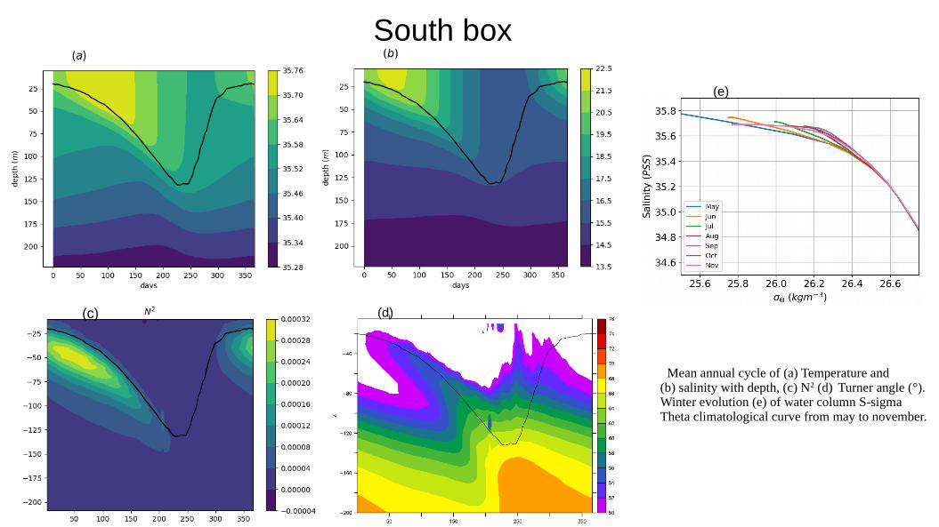
Mean annual cycle of (a) Temperature and(b) salinity with depth, (c) N2 (d) Turner angle (°).Winter evolution (e) of water column S-sigma Theta climatological curve from may to november.

(c) (d)

(e)

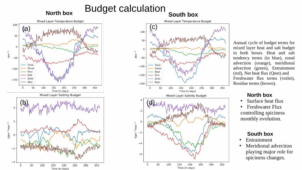
Budget calculationNorth box South box

(a)

(b)

(c)

(d)

Annual cycle of budget terms for mixed layer heat and salt budget in both boxes. Heat and salt tendency terms (in blue), zonal advection (orange), meridional advection (green), Entrainment (red), Net heat flux (Qnet) and Freshwater flux terms (voilet), Residue terms (brown).

North box● Surface heat flux● Freshwater Fluxcontrolling spiciness monthly evolution.

South box● Entrainment● Meridional advection

playing major role for spiciness changes.