第 4 章 常用的 r 內建 4: common r computing...
TRANSCRIPT

第 4 章: 常用的 R 內建函式
4: Common R Computing Functions
4.1 函式的語法
R 向量的算數操作, 有許多時候透過 “函式” (function). 一個函數是通過下面的語句形式定義:
> name <- function(arg_1, arg_2, ...) expression
多數含函式進行計算產生結果, 回傳一個 R 的物件, 有些用來進行特殊繪圖與列印. 一個函式內通常需
輸入 引數 (argument), 引數可以是一個以上, 有些引數一定要輸入 (required argument), 有些引數
可以不用輸入 (optional argument), 有些引數附有一個 = (等號), 可以直接使用 R 的內部設定值.
> x<-1:10
> max(x)
[1] 10
> min(x)
[1] 1
> log(x)
[1] 0.0000000 0.6931472 1.0986123 1.3862944 1.6094379 1.7917595
[7] 1.9459101 2.0794415 2.1972246 2.3025851
> mean(x)
[1] 5.5
> sd(x)
[1] 3.027650
> summary(x)
Min. 1st Qu. Median Mean 3rd Qu. Max.
1.00 3.25 5.50 5.50 7.75 10.00
許多時候, 可以在 R輸入函式名稱, 查看函式的內容與計算過程. 如指令提示下輸入 sd
> sd
function (x, na.rm = FALSE)
if (is.matrix(x))
apply(x, 2, sd, na.rm = na.rm)
else if (is.vector(x))
c©林建甫 (October 27, 2006)

· 2 · 4.2 算數函式
sqrt(var(x, na.rm = na.rm))
else if (is.data.frame(x))
sapply(x, sd, na.rm = na.rm)
else sqrt(var(as.vector(x), na.rm = na.rm))
4.2 算數函式 Arithmethic Computing
R 有許多內建算數函式, 包含各種三角函式, 詳見表 4.1
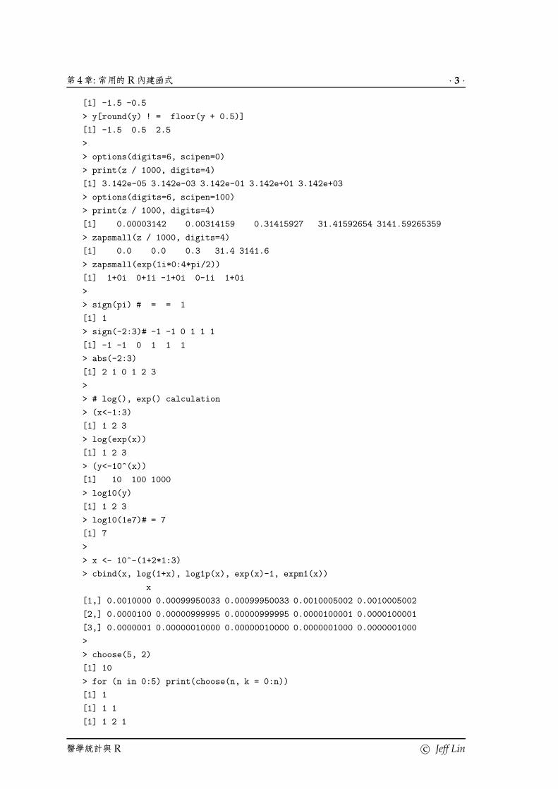
> # Arithmethic Computing
> # rounding
> (x<- 0.5 + -2:4)
[1] -1.5 -0.5 0.5 1.5 2.5 3.5 4.5
> round(x) # IEEE rounding: -2 0 0 2 2 4 4
[1] -2 0 0 2 2 4 4
> (y<-seq(-2, 4, by = 0.5))
[1] -2.0 -1.5 -1.0 -0.5 0.0 0.5 1.0 1.5 2.0 2.5 3.0 3.5 4.0
> (y.round<-round(y)) #-- IEEE rounding !
[1] -2 -2 -1 0 0 0 1 2 2 2 3 4 4
> (y.trunc<-trunc(y))
[1] -2 -1 -1 0 0 0 1 1 2 2 3 3 4
> (y.signif<-signif(y))
[1] -2.0 -1.5 -1.0 -0.5 0.0 0.5 1.0 1.5 2.0 2.5 3.0 3.5 4.0
> (y.ceil<-ceiling(y))
[1] -2 -1 -1 0 0 1 1 2 2 3 3 4 4
> (y.floor<-floor(y))
[1] -2 -2 -1 -1 0 0 1 1 2 2 3 3 4
> cbind(y,y.round, y.trunc, y.signif, y.ceil, y.floor)
y y.round y.trunc y.signif y.ceil y.floor
[1,] -2.0 -2 -2 -2.0 -2 -2
[2,] -1.5 -2 -1 -1.5 -1 -2
[3,] -1.0 -1 -1 -1.0 -1 -1
[4,] -0.5 0 0 -0.5 0 -1
[5,] 0.0 0 0 0.0 0 0
[6,] 0.5 0 0 0.5 1 0
[7,] 1.0 1 1 1.0 1 1
[8,] 1.5 2 1 1.5 2 1
[9,] 2.0 2 2 2.0 2 2
[10,] 2.5 2 2 2.5 3 2
[11,] 3.0 3 3 3.0 3 3
[12,] 3.5 4 3 3.5 4 3
[13,] 4.0 4 4 4.0 4 4
>
> y[trunc(y) ! = floor(y)]
c© Jeff Lin 醫學統計與 R
第 4 章: 常用的 R 內建函式 · 3 ·
[1] -1.5 -0.5
> y[round(y) ! = floor(y + 0.5)]
[1] -1.5 0.5 2.5
>
> options(digits=6, scipen=0)
> print(z / 1000, digits=4)
[1] 3.142e-05 3.142e-03 3.142e-01 3.142e+01 3.142e+03
> options(digits=6, scipen=100)
> print(z / 1000, digits=4)
[1] 0.00003142 0.00314159 0.31415927 31.41592654 3141.59265359
> zapsmall(z / 1000, digits=4)
[1] 0.0 0.0 0.3 31.4 3141.6
> zapsmall(exp(1i*0:4*pi/2))
[1] 1+0i 0+1i -1+0i 0-1i 1+0i
>
> sign(pi) # = = 1
[1] 1
> sign(-2:3)# -1 -1 0 1 1 1
[1] -1 -1 0 1 1 1
> abs(-2:3)
[1] 2 1 0 1 2 3
>
> # log(), exp() calculation
> (x<-1:3)
[1] 1 2 3
> log(exp(x))
[1] 1 2 3
> (y<-10^(x))
[1] 10 100 1000
> log10(y)
[1] 1 2 3
> log10(1e7)# = 7
[1] 7
>
> x <- 10^-(1+2*1:3)
> cbind(x, log(1+x), log1p(x), exp(x)-1, expm1(x))
x
[1,] 0.0010000 0.00099950033 0.00099950033 0.0010005002 0.0010005002
[2,] 0.0000100 0.00000999995 0.00000999995 0.0000100001 0.0000100001
[3,] 0.0000001 0.00000010000 0.00000010000 0.0000001000 0.0000001000
>
> choose(5, 2)
[1] 10
> for (n in 0:5) print(choose(n, k = 0:n))
[1] 1
[1] 1 1
[1] 1 2 1
醫學統計與 R c© Jeff Lin

· 4 · 4.2 算數函式
[1] 1 3 3 1
[1] 1 4 6 4 1
[1] 1 5 10 10 5 1
>
> # combination
> factorial(100)
[1] 9.33262e+157
> lfactorial(10000)
[1] 82109
>
> (x.tri<-c(0, pi/2, pi, 3*pi/2))
[1] 0.00000 1.57080 3.14159 4.71239
> sin(x.tri)
[1] 0.000000000000000000000 1.000000000000000000000
[3] 0.000000000000000122461 -1.000000000000000000000
> asin(sin(x.tri))
[1] 0.000000000000000000000 1.570796326794896600000
[3] 0.000000000000000122461 -1.570796326794896600000
c© Jeff Lin 醫學統計與 R

第 4 章: 常用的 R 內建函式 · 5 ·
表 4.1: 常見數學函式
函式 說明
? Help
<- Left assignment, binary
-> Right assignment, binary
$ List subset, binary
: Sequence, binary
: In model formulae: interaction
~ Tilde, used for model formulae, can be either uniary or binary
- Substraction, can be unary or binary
+ Addition, can be unary or binary
! Unary not
* Multiplication, binary
/ Division, binary
^ Exponentiation, binary
%% Modulus, binary
%/% Integer divide, binary
round(x, digits = 0) its first argument to the specified number of decimal places
signif(x, digits = 6) rounds the values to the specified number of significant digits
trunc(x) the integers by truncating ’x’ toward ’0’
ceiling(x) the smallest integers not less than ’x’
floor(x) the largest integers not greater than ’x’
sign(x) sign(x), the sign of a real number is 1, 0, or -1
if the number is positive, zero, or negative, respectively.
abs(x) |x|, absolute value of x
sqrt(x)√
x
exp(x) ex
expm1(x) computes exp(x) − 1 accurately also for |x| << 1.
log(x) log(x)
log10(x) log10(x)
log2(x) log2(x)
logb(x, base = z) logz(x)
log1p(x) computes log(1 + x) accurately also for |x| << 1.
gamma(x) Γ(x) = (x − 1)! =∫ ∞
0 t(x−1) exp(−t)dt
lgamma(x) loge[Γ(x)]
beta(a, b) B(a, b) = (Γ(a)Γ(b)) / (Γ(a + b)) =∫ 1
0 t(a−1)(1 − t)(b−1)dt
lbeta(a, b) loge[B(a, b)]
digamma(x) ddx loge[Γ(x)]
trigamma(x) d2
dx2 loge[Γ(x)]
psigamma(x, deriv = 0) dp
dxp loge[Γ(x)]
choose(n, k) n!k! (n−k)!
lchoose(n, k) loge(choose(n, k))
factorial(x) x! = Γ(x + 1)
lfactorial(x) log(x!) = loge[Γ(x)]
sin(x) cos(x) tan(x) trigonometric functions
asin(x) acos(x) atan(x) inverse functions
sinh(x) cosh(x) tanh(x) hyperbolic functionsx
asinh(x) acosh(x) atanh(x) inverse hyperbolic functions
醫學統計與 R c© Jeff Lin
· 6 · 4.3 all(), any(), which()
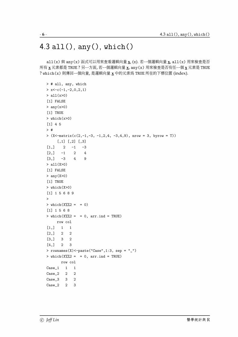
4.3 all(), any(), which()
all(x)與 any(x) 函式可以用來查看邏輯向量 x, (x). 若一個邏輯向量 x, all(x) 用來檢查是否
所有 x 元素都是 TRUE ? 另一方面,若一個邏輯向量 x, any(x) 用來檢查是否有任一個 x 元素是 TRUE
? which(x) 則傳回一個向量, 是邏輯向量 x 中的元素為 TRUE 所在的下標位置 (index).
> # all, any, which
> x<-c(-1,-2,0,2,1)
> all(x>0)
[1] FALSE
> any(x>0)
[1] TRUE
> which(x>0)
[1] 4 5
> #
> (X<-matrix(c(2,-1,-3, -1,2,4, -3,4,9), nrow = 3, byrow = T))
[,1] [,2] [,3]
[1,] 2 -1 -3
[2,] -1 2 4
[3,] -3 4 9
> all(X>0)
[1] FALSE
> any(X>0)
[1] TRUE
> which(X>0)
[1] 1 5 6 8 9
>
> which(X%%2 = = 0)
[1] 1 5 6 8
> which(X%%2 = = 0, arr.ind = TRUE)
row col
[1,] 1 1
[2,] 2 2
[3,] 3 2
[4,] 2 3
> rownames(X)<-paste("Case",1:3, sep = "_")
> which(X%%2 = = 0, arr.ind = TRUE)
row col
Case_1 1 1
Case_2 2 2
Case_3 3 2
Case_2 2 3
c© Jeff Lin 醫學統計與 R

第 4 章: 常用的 R 內建函式 · 7 ·
4.4 排序函式 Ranking and Sorting
在 R 中有數個與排序相關的函式, 如 rev(), sort(), order() 與 rank(). z<-rev(x) 回傳
一個向量 z, 是將向量 x 元素反轉; z<-rank(x) 回傳一個向量 z, 是將向量 x 每一個元素從小到大排
序之後, x 元素之相對順序 (rank); z<-sort(x) 回傳一個向量 z, 是將向量 x 從小到大排序的結果;
z<-order(x) 回傳一個向量 z, 是將向量 x 從小到大排序後的向量之元素, 在原來向量 x 的原始位
置.
> x<-c(7,9,6,10,8)
> rev(x)
[1] 8 10 6 9 7
> rank(x)
[1] 2 4 1 5 3
> sort(x) # from the smallest to the largest
[1] 6 7 8 9 10
> order(x) # x[3] is the smallest one.
[1] 3 1 5 2 4
當向量內元數有相同的數值時, 在 rank() 內引數 ties.method, 可以輸入各種相同的數值時排序的
選擇, 如 ties.method = c("average", "first", "random", "max", "min").
> x<-c(7,9,6,7,8)
> rank(x, ties.method = "average")
[1] 2.5 5.0 1.0 2.5 4.0
> sort(x)
[1] 6 7 7 8 9
> order(x)
[1] 3 1 4 5 2
在統計分析中, 常須對矩陣或資料框架中的某些變數做排序, 可以利用 order().
> (x<-c(1, 1, 3:1, 1:4, 3))
[1] 1 1 3 2 1 1 2 3 4 3
> (y<-c(9, 9:1))
[1] 9 9 8 7 6 5 4 3 2 1
> (z<-c(2, 1:9))
[1] 2 1 2 3 4 5 6 7 8 9
> (xyz.mat<-rbind(x,y,z))
[,1] [,2] [,3] [,4] [,5] [,6] [,7] [,8] [,9] [,10]
x 1 1 3 2 1 1 2 3 4 3
y 9 9 8 7 6 5 4 3 2 1
z 2 1 2 3 4 5 6 7 8 9
> xyz.order<-order(x,y,z)
> xyz.mat[, xyz.order] # reordering (ties via 2nd & 3rd arg)
[,1] [,2] [,3] [,4] [,5] [,6] [,7] [,8] [,9] [,10]
x 1 1 1 1 2 2 3 3 3 4
y 5 6 9 9 4 7 1 3 8 2
醫學統計與 R c© Jeff Lin
· 8 · 4.4 排序函式
z 5 4 1 2 6 3 9 7 2 8
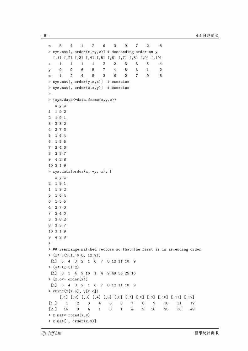
> xyz.mat[, order(x,-y,z)] # descending order on y
[,1] [,2] [,3] [,4] [,5] [,6] [,7] [,8] [,9] [,10]
x 1 1 1 1 2 2 3 3 3 4
y 9 9 6 5 7 4 8 3 1 2
z 1 2 4 5 3 6 2 7 9 8
> xyz.mat[, order(y,z,x)] # exercise
> xyz.mat[, order(z,x,y)] # exercise
>
> (xyz.data<-data.frame(x,y,z))
x y z
1 1 9 2
2 1 9 1
3 3 8 2
4 2 7 3
5 1 6 4
6 1 5 5
7 2 4 6
8 3 3 7
9 4 2 8
10 3 1 9
> xyz.data[order(x, -y, z), ]
x y z
2 1 9 1
1 1 9 2
5 1 6 4
6 1 5 5
4 2 7 3
7 2 4 6
3 3 8 2
8 3 3 7
10 3 1 9
9 4 2 8
>
> ## rearrange matched vectors so that the first is in ascending order
> (x<-c(5:1, 6:8, 12:9))
[1] 5 4 3 2 1 6 7 8 12 11 10 9
> (y<-(x-5)^2)
[1] 0 1 4 9 16 1 4 9 49 36 25 16
> (z.o<- order(x))
[1] 5 4 3 2 1 6 7 8 12 11 10 9
> rbind(x[z.o], y[z.o])
[,1] [,2] [,3] [,4] [,5] [,6] [,7] [,8] [,9] [,10] [,11] [,12]
[1,] 1 2 3 4 5 6 7 8 9 10 11 12
[2,] 16 9 4 1 0 1 4 9 16 25 36 49
> z.mat<-rbind(x,y)
> z.mat[ , order(x,y)]
c© Jeff Lin 醫學統計與 R

第 4 章: 常用的 R 內建函式 · 9 ·
[,1] [,2] [,3] [,4] [,5] [,6] [,7] [,8] [,9] [,10] [,11] [,12]
x 1 2 3 4 5 6 7 8 9 10 11 12
y 16 9 4 1 0 1 4 9 16 25 36 49
表 4.2 摘要常見的常見排序函式.
表 4.2: 常見之排序函式
函式 說明
rev(x) reverse order
rank(x) Returns the sample ranks of the values
Default argument” ties.method = "average"
sort(x) Sort a vector or factor (partially)
into ascending (or descending) order.
order(x) Returns a permutation
which rearranges its first argument into ascending
or descending order, breaking ties by further arguments.
4.5 常用之文字函式 Functinos for Characters
R 內有許多函數可以處理文字型態的資料物件 (Character Data), 常用之文字函式有 paste(),
substr(), substring(), grep()等.
4.5.1 paste() 函式
paste(..., sep = " ") 函式可以合併 2 個文字向量中的元素使其合而為 1 個文字向量, 其中
2 個文字字串合併中間分隔使用文字或符號 "text", 可以用引數 sep="text";若要 2 個文字向量合
併中間分隔使用文字或符號 "text", 且合併後成為單一文字字串, 可以用引數 collapse="text" .
> # paste
> paste(1:5) # same as as.character(1:5)
[1] "1" "2" "3" "4" "5"
> paste("A", 1:5, sep = "")
[1] "A1" "A2" "A3" "A4" "A5"
> paste("A", 1:5, sep = " ")
[1] "A 1" "A 2" "A 3" "A 4" "A 5"
> paste("A", 1:5, sep = "#")
[1] "A#1" "A#2" "A#3" "A#4" "A#5"
> paste("Today is", date())
[1] "Today is Fri Oct 27 09:37:44 2006"
> #
醫學統計與 R c© Jeff Lin

· 10 · 4.5 常用之文字函式
> paste(c("X", "Y"), 1:5)
[1] "X 1" "Y 2" "X 3" "Y 4" "X 5"
> paste(c("X", "Y"), 1:5, sep = " ")
[1] "X 1" "Y 2" "X 3" "Y 4" "X 5"
> paste(c("X", "Y"), 1:5, sep = "")
[1] "X1" "Y2" "X3" "Y4" "X5"
> paste(c("X", "Y"), 1:5, sep = "+")
[1] "X+1" "Y+2" "X+3" "Y+4" "X+5"
> paste(c("X", "Y"), 1:5, sep = "", collapse=" + ")
[1] "X1 + Y2 + X3 + Y4 + X5"
4.5.2 substr() 與 substring() 函式
substr(), substring() 函式可在 1 個文字向量中, 萃取傳回部分的字串.
substr(x.char, start, stop)
x.char 為 1 個向文字字串向量, start, 為 1 個正整數, 表示所要萃取文字字串的第 1 個文字
位置, stop, 為 1 個正整數,表示所要萃取文字字串的最後 1 個文字位置. 例如 R 內建之料框架
state,關於美國 50 洲的一些相關資料, 使用substring() 函式.
substring(x.text, first, last = 1000000)
x.text 為 1 個向文字字串向量, first, 為 1 個正整數, 表示所要萃取文字字串的第 1 個文字
位置, last, 為 1 個正整數,表示所要萃取文字字串的最後 1 個文字位置. 例如 R 內建之料框架
state,關於美國 50 洲的一些相關資料, 使用substring() 函式.
用其它文字字串來取代原先所萃取之文字字串
若用 substr(x.char, start, stop)<-new.char
或 substring(x.text, first, last = 1000000)<-new.text
可以指派新的文字字串 new.char 或 new.text 取代原先所萃取之文字字串之位置.
> # substr()
> data(state)
> state.name[47:50]
[1] "Washington" "West Virginia" "Wisconsin" "Wyoming"
> substr(state.name[47:50], 1, 4)
[1] "Wash" "West" "Wisc" "Wyom"
>
> substr(state.name[47:50], 1, 4)<-"AAA"
> state.name[47:50]
[1] "AAAhington" "AAAt Virginia" "AAAconsin" "AAAming"
>
>
> # substring()
> data(state)
> state.name[47:50]
[1] "Washington" "West Virginia" "Wisconsin" "Wyoming"
c© Jeff Lin 醫學統計與 R
第 4 章: 常用的 R 內建函式 · 11 ·
> substring(state.name[47:50], first=3, last=1000)
[1] "shington" "st Virginia" "sconsin" "oming"
>
> substring(state.name[47:50], first=3, last=1000)<-"BBB"
> state.name[47:50]
[1] "WaBBBngton" "WeBBBVirginia" "WiBBBnsin" "WyBBBng"
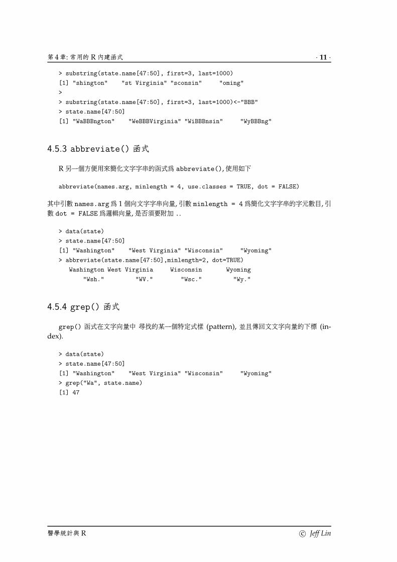
4.5.3 abbreviate() 函式
R 另一個方便用來簡化文字字串的函式為 abbreviate(), 使用如下
abbreviate(names.arg, minlength = 4, use.classes = TRUE, dot = FALSE)
其中引數 names.arg為 1 個向文字字串向量, 引數 minlength = 4 為簡化文字字串的字元數目, 引
數 dot = FALSE 為邏輯向量, 是否須要附加 ..
> data(state)
> state.name[47:50]
[1] "Washington" "West Virginia" "Wisconsin" "Wyoming"
> abbreviate(state.name[47:50],minlength=2, dot=TRUE)
Washington West Virginia Wisconsin Wyoming
"Wsh." "WV." "Wsc." "Wy."
4.5.4 grep() 函式
grep() 函式在文字向量中 尋找的某一個特定式樣 (pattern), 並且傳回文文字向量的下標 (in-
dex).
> data(state)
> state.name[47:50]
[1] "Washington" "West Virginia" "Wisconsin" "Wyoming"
> grep("Wa", state.name)
[1] 47
醫學統計與 R c© Jeff Lin

· 12 · 4.6 日期函式
4.6 日期函式 Date Function
時間在醫學研究中, 是一個非常重要的變數, 然而對時間的儲存, 列印與計算, 每一個軟體各不相
同的處理方法. 原則上, 軟體對時間的輸入通常是文字型式的日歷時間 (Calendar date and time),
如 "12/10/1979" "12/10/1979 20:30:10", "2/28/1947", "2-28-1947", 022847, 2Feb47,
"Feburary 2 1947"等, R 讀入文字型式的日歷時間, 轉換成 R 的 “日期-時間類別物件 (date-time
class object). as.Date() 函式將文字型式的日歷 (calendar date) 轉換成 R 的 “日期類別物件”
(Date class object); strptime() 函式將文字型式的日歷時間轉換成 R 的 “日期-時間類別物件”;
as.POSIXlt()與 as.POSIXct() 函式將 “日期-時間類別物件”轉換成 POSIXlt, POSIXct 格式.
format() 函式將 R 的 “日期-時間類別物件” 轉換成一般人可讀的文字型式的日期, 日, 星期, 月, 與
時間.
4.6.1 as.Date() 函式
as.Date() 函式將文字型式的日歷 (calendar date) 轉換成 R 的 “日期類別物件”, 日期類別
物件是一個擁有 Date class 數值型的向量. 在 R 中, 數值型的 Date class 向量是以 Januayr
1, 1970 為 0, 以稱做 Julian Date. 轉換後的標準格式是 yyyy-mm-dd, 若要看數值型的 Julian 格
式, 可用 as,numeric() 或 julian(). POSIXlt 物件格式表示 R 使用可讀的列表物件 (lt: legi-
ble time), POSIXct 格式表示 R 使用連續型時間計算的數值格式 (ct: continuous time), 可以用
as.numeric() 函式,轉換成以 Januayr 1, 1970, 0 時, 0 分 為 “0”, 時間零點, 加以計算.
> # Date
> x.date<-c("2/28/1947", "12/10/1979", "1/1/1970")
> x.date
[1] "2/28/1947" "12/10/1979" "1/1/1970"
> #convert to Julian dates
> x.julian<-as.Date(x.date, format = "%m/%d/%Y")
> x.julian
[1] "1947-02-28" "1979-12-10" "1970-01-01"
> #display Julian dates as a numerical vector
> as.numeric(x.julian)
[1] -8343 3630 0
> julian(x.julian)
[1] -8343 3630 0
attr(,"origin")
[1] "1970-01-01"
>
> # as.POSIXlt and as.POSIXct Object
> as.POSIXlt(x.julian)
[1] "1947-02-28" "1979-12-10" "1970-01-01"
> as.numeric(as.POSIXlt(x.julian))
錯誤在 as.double.default(as.POSIXlt(x.julian)) :
(串列) 目的物件不能強制變更成 double
> as.POSIXct(x.julian)
c© Jeff Lin 醫學統計與 R

第 4 章: 常用的 R 內建函式 · 13 ·
[1] "1947-02-28 08:00:00 台北標準時間"
[2] "1979-12-10 08:00:00 台北標準時間"
[3] "1970-01-01 08:00:00 台北標準時間"
> as.numeric(as.POSIXct(x.julian))
[1] -720835200 313632000 0
weekdays(), months(), quarters(), julian()等函式, 可以取的日期類別物件的訊息.
> # Julian
> weekdays(x.julian)
[1] "星期五" "星期一" "星期四"
> weekdays(x.julian, abbreviate = TRUE)
[1] "星期五" "星期一" "星期四"
> months(x.julian, abbreviate = FALSE)
[1] "二月" "十二月" "一月"
> quarters(x.julian, abbreviate = TRUE)
[1] "Q1" "Q4" "Q1"
> julian(x.julian)
[1] -8343 3630 0
attr(,"origin")
[1] "1970-01-01"
codeSys.Date() 可以取得電腦今天的日期, 用來計算年紀.
> # calculate age as of today’s date
> date.today<-Sys.Date()
> x.age.error<-(date.today-x.julian)/365.25
> x.age.error
Time differences of 59.5510, 26.7707, 36.7091 days
> # #the display of ’days’ is not correct
> # truncate number to get "age"
> x.age.correct<-trunc(as.numeric(x.age))
> x.age.correct
[1] 59 26 36
> # create data frame
> x.data<-data.frame(Birthday = x.date,
Standard = x.julian,
Julian = as.numeric(x.julian),
Age = x.age.correct)
> x.data
Birthday Standard Julian Age
1 2/28/1947 1947-02-28 -8343 59
2 12/10/1979 1979-12-10 3630 26
3 1/1/1970 1970-01-01 0 36
醫學統計與 R c© Jeff Lin

· 14 · 4.6 日期函式
4.6.2 日期與時間之格式 (Format)
文字型式的日歷 (calendar date) 以各種不同型式輸入, 所以有時須要用 as.Date() 函式中的引
數 format 做適當之轉換, 注意, 使用中文介面, as.Date() 有些時候無法讀出正確日期. 須對系統做
些調整. 見表 4.3, 或輔助文件: help(strptime).
> ######### date with input format
> as.Date("1990-1-19") # standard format
[1] "1990-01-19"
> as.Date("9/15/89", format = "%m/%d/%y") # two digits for year
[1] "1989-09-15"
> as.Date("4 25 92", format = "%m %d %y")
[1] "1992-04-25"
> as.Date("063095", format = "%m%d%y")
[1] "1995-06-30"
>
> # chinese GUI cause problems
> as.Date("September 15, 1995", format = "%B %d, %Y")
[1] NA
> as.Date("27Aug95", format = "%d%b%y") # two digits for year
[1] NA
> as.Date("27Aug1995", format = "%d%b%Y")
[1] NA
> as.Date("September 15 1995", format = "%B %d %Y")
[1] NA
>
> ## read in date info in format ’ddmmmyyyy’
> ## This will give NA(s) in some locales; setting the C locale
> ## as in the commented lines will overcome this on most systems.
>
> # check local setting
> ## locale-specific version of date()
> format(Sys.time(), "%a %b %d %X %Y %Z")
[1] "星期日 九月 17 上午 10:56:11 2006 台北標準時間"
>
> # change it
> (lct <- Sys.getlocale("LC_TIME"))
[1] "Chinese_Taiwan.950"
> Sys.setlocale("LC_TIME", "C")
[1] "C"
> format(Sys.time(), "%a %b %d %X %Y %Z")
[1] "Sun Sep 17 10:56:11 2006 台北標準時間"
>
> # read it again
> as.Date("September 15, 1995", format = "%B %d, %Y")
[1] "1995-09-15"
c© Jeff Lin 醫學統計與 R
第 4 章: 常用的 R 內建函式 · 15 ·
> as.Date("27Aug95", format = "%d%b%y") # two digits for year
[1] "1995-08-27"
> as.Date("27Aug1995", format = "%d%b%Y")
[1] "1995-08-27"
> as.Date("September 15 1995", format = "%B %d %Y")
[1] "1995-09-15"
> Sys.setlocale("LC_TIME", lct)
[1] "Chinese_Taiwan.950"
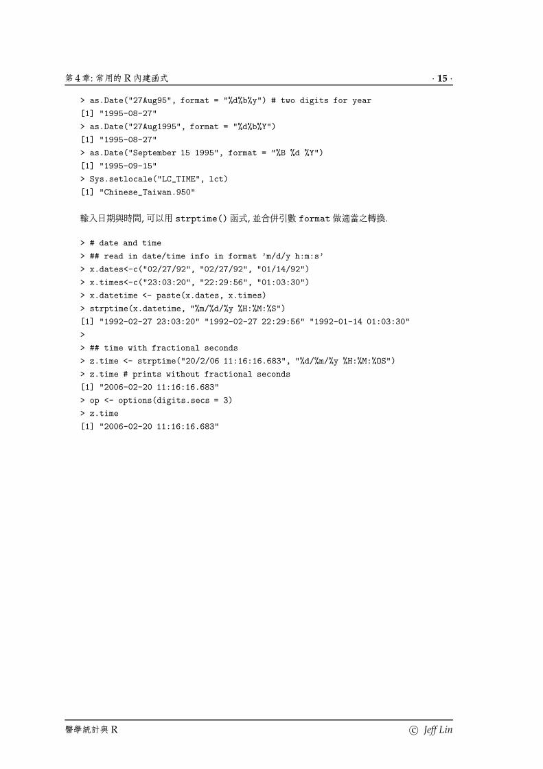
輸入日期與時間, 可以用 strptime() 函式, 並合併引數 format 做適當之轉換.
> # date and time
> ## read in date/time info in format ’m/d/y h:m:s’
> x.dates<-c("02/27/92", "02/27/92", "01/14/92")
> x.times<-c("23:03:20", "22:29:56", "01:03:30")
> x.datetime <- paste(x.dates, x.times)
> strptime(x.datetime, "%m/%d/%y %H:%M:%S")
[1] "1992-02-27 23:03:20" "1992-02-27 22:29:56" "1992-01-14 01:03:30"
>
> ## time with fractional seconds
> z.time <- strptime("20/2/06 11:16:16.683", "%d/%m/%y %H:%M:%OS")
> z.time # prints without fractional seconds
[1] "2006-02-20 11:16:16.683"
> op <- options(digits.secs = 3)
> z.time
[1] "2006-02-20 11:16:16.683"
醫學統計與 R c© Jeff Lin

· 16 · 4.6 日期函式
表 4.3: 常見日期與時間之格式
格式 說明
%a Abbreviated weekday name
%A Full weekday name
%b Abbreviated month name
%B Full month name
%c Date and time, locale-specific.
%d Day of the month as decimal number (01-31).
%H Hours as decimal number (00-23).
%I Hours as decimal number (01-12).
%j Day of year as decimal number (001-366).
%m Month as decimal number (01-12).
%M Minute as decimal number (00-59).
%p AM/PM indicator in the locale.
Used in conjuction with ’%I’ and *not* with ’%H’.
%S Second as decimal number (00-61), allowing for up to two leap-seconds
%U Week of the year as decimal number (00-53)
using the first Sunday as day 1 of week 1.
%w Weekday as decimal number (0-6, Sunday is 0).
%W Week of the year as decimal number (00-53)
using the first Monday as day 1 of week 1.
%x Date, locale-specific.
%X Time, locale-specific.
%y Year without century (00-99).
If you use this on input, which century you get is system-specific. So don’t!
Often values up to 69 (or 68) are prefixed by 20 and 70-99 by 19.
%Y Year with century.
%z (output only.) Offset from Greenwich, so ’-0800’ is 8 hours west of Greenwich.
%Z (output only.) Time zone as a character string (empty if not available).
%F Equivalent to %Y-%m-%d (the ISO 8601 date format).
%g The last two digits of the week-based year (see ’%V’).
%G The week-based year (see ’%V’) as a decimal number.
%u Weekday as a decimal number (1-7, Monday is 1).
%V Week of the year as decimal number (00-53).
If the week (starting on Monday) containing 1 January
has four or more days in the new year, then it is considered week 1.
Otherwise, it is the last week of the previous year,
and the next week is week 1.
%D Locale-specific date format such as ’%m/%d/%y’.
%k The 24-hour clock time with single digits preceded by a blank.
%l The 12-hour clock time with single digits preceded by a blank.
%n Newline on output, arbitrary whitespace on input.
%r The 12-hour clock time (using the locale’s AM or PM).
%R Equivalent to ’%H:%M’.
%t Newline on output, arbitrary whitespace on input.
%T Equivalent to ’%H:%M:%S’.
c© Jeff Lin 醫學統計與 R

第 4 章: 常用的 R 內建函式 · 17 ·
4.6.3 survival 套件常用日期與時間函式
survival 套件有一些常用日期與時間之函式, 如 as.date(), 函式類似 as.Date(), 可以讀入
9/15/89, 9-1-1990, 4 25 92, 063095, 27Aug95, or September 15 1995等格式. 但是轉換成
以 Januay 1, 1960, 0 時, 0 分 為 “0”, 時間零點, 加以計算, (與 SAS 相同).
> # "survival" package
> # as.date() without input format
> as.date(c("28feb1947", "December 10 1979", "1Jan1970"))
[1] 28Feb47 10Dec79 1Jan70
> as.date("9/15/89")
[1] 15Sep89
> as.date("9-1-1990")
[1] 1Sep90
> as.date("4 25 92")
[1] 25Apr92
> as.date("063095")
[1] 30Jun95
> as.date("27Aug95")
[1] 27Aug95
> as.date("September 15 1995")
[1] 15Sep95
>
> # survival package continuous time: day zero
> as.numeric(as.date("1/1/1960"))
[1] 0
> as.numeric(as.date("1/1/1970"))
[1] 3653
>
> # base package continuous time
> as.numeric(as.Date("1960-1-1"))
[1] -3653
> as.numeric(as.Date("1970-1-1"))
[1] 0
mdy.date(), 函式將個別代表 月份 (months), 日期 (days), 年代 (years) 的向量, 合併成 R 的
日期物件.
> # mdy.date()
> mons<-c(2, 12, 5, 9)
> days<-c(28, 10, 20, 9)
> years<-c(1947, 1979, 2000, 2006)
> s.date<-mdy.date(mons, days, years)
> s.date
[1] 28Feb47 10Dec79 20May2000 9Sep2006
> as.numeric(s.date)
[1] -4690 7283 14750 17053
醫學統計與 R c© Jeff Lin

· 18 · 4.7 敘述性統計函式
date.mdy() 函式將 R 的日期物件轉換成個別代表 月份 (months), 日期 (days), 年代 (years)
的列表物件
> # date.mdy()
> s.date
[1] 28Feb47 10Dec79 20May2000 9Sep2006
> date.mdy(s.date)
$month
[1] 2 12 5 9
$day
[1] 28 10 20 9
$year
[1] 1947 1979 2000 2006
> #
> date.mdy(s.date, weekday = T)
$month
[1] 2 12 5 9
$day
[1] 28 10 20 9
$year
[1] 1947 1979 2000 2006
$weekday
[1] 6 2 7 7
date.mmddyy(), date.ddmmyy(), date.mmddyyyy() 函式將 R 的日期物件做格式化 (for-
mat) 或不同的日期物件格式做轉換.
> # date.mmddyy(), date.ddmmmyy(), date.mmddyyyy()
> date.mmddyy(s.date)
[1] "2/28/47" "12/10/79" "5/20/2000" "9/9/2006"
> date.ddmmmyy(s.date)
[1] "28Feb47" "10Dec79" "20May2000" "9Sep2006"
> date.mmddyyyy(s.date)
[1] "2/28/1947" "12/10/1979" "5/20/2000" "9/9/2006"
4.7 統計函式 Descriptive Statistics Functions
R 有許多統計函式, 對向量物件常見的基礎敘述統計量, 如 sum(), cumsum(), diff(), prod(),
cumprod(), mean(), median(), var(), sd(), range(), min(), max(), quantile(), sample(x)
等. 參見表 4.4. 注意, 若物件中有缺失值, 須作特別處裡, 可用 mean(na.omit(x)) 或 mean(x,
na.rm = T) 引數. 另外對矩陣或資料框架物件做運算, 會有不預期的結果,須小心.
y<-sum(x) 函式是 y = ∑i xi; z<-cums(x) 函式是 zj = ∑i≤j xi; z<-diff(x) 函式是 zi =
xi+1 − xi.
同樣的, <-prod(x) 函式是 y = ∏i xi; z<-cumprod(x) 函式是 zj = ∏i≤j xi; 平均值是
c© Jeff Lin 醫學統計與 R

第 4 章: 常用的 R 內建函式 · 19 ·
xbar<-mean(x), (x̄ = 1n ∑i xi); 中位數是 x.med<-median(x), (0.5 quantile, 50th percentile);
變異數是 x.s2<-var(x), s2 = 1n−1 ∑i(xi − x̄)2; 標準差是 x.sd<-sd(x), s =
√s2; z<-range(x)
函式回傳一個向量,二個元素 [min(x), max(x)]; 極大值與極小值分別為 min(x), max(x); 取的百分
位值可以用 quantile(), 如 quantile(x, probs = c(0.05, 0.25, 0.5, 0.75, 0.95)).
fivenum(x) 回傳向量 [max, Q1, median, Q3, max].
> # STAT
> (x<-seq(-2, 3, 0.3))
[1] -2.0 -1.7 -1.4 -1.1 -0.8 -0.5 -0.2 0.1 0.4 0.7 1.0 1.3 1.6
[14] 1.9 2.2 2.5 2.8
> sum(x)
[1] 6.8
> cumsum(x)
[1] -2.0 -3.7 -5.1 -6.2 -7.0 -7.5 -7.7 -7.6 -7.2 -6.5 -5.5 -4.2 -2.6
[14] -0.7 1.5 4.0 6.8
> diff(x)
[1] 0.3 0.3 0.3 0.3 0.3 0.3 0.3 0.3 0.3 0.3 0.3 0.3 0.3 0.3 0.3 0.3
> prod(x)
[1] -0.713814
> cumprod(x)
[1] -2.0000000 3.4000000 -4.7600000 5.2360000 -4.1888000 2.0944000
[7] -0.4188800 -0.0418880 -0.0167552 -0.0117286 -0.0117286 -0.0152472
[13] -0.0243956 -0.0463516 -0.1019735 -0.2549337 -0.7138144
> mean(x)
[1] 0.4
> median(x)
[1] 0.4
> var(x)
[1] 2.295
> sd(x)
[1] 1.51493
> range(x)
[1] -2.0 2.8
> min(x)
[1] -2
> max(x)
[1] 2.8
> (y<-quantile(x, probs = c(0.05, 0.25, 0.5, 0.75, 0.95)))
5% 25% 50% 75% 95%
-1.76 -0.80 0.40 1.60 2.56
> # quantile range
> y[4]-y[2]
75%
2.4
>
> y[4]-y[2]
醫學統計與 R c© Jeff Lin

· 20 · 4.7 敘述性統計函式
75%
2.4
>
> fivenum(x)
[1] -2.0 -0.8 0.4 1.6 2.8
>
> # missing values
> x[3]<-NA
> x[7]<-NA
> x
[1] -2.0 -1.7 NA -1.1 -0.8 -0.5 NA 0.1 0.4 0.7 1.0 1.3 1.6
[14] 1.9 2.2 2.5 2.8
> mean(x)
[1] NA
> mean(na.omit(x))
[1] 0.56
> var(x, na.rm = T)
[1] 2.33829
表 4.4: 常見敘述性統計函式
格式 說明
sum(x) summation y = ∑i xi
cumsum(x) cumulative sum zj = ∑i≤j xi
diff(x) x[i+1]-x[i] zi = xi+1 − xi
prod(x) product y = ∏i xi
cumprod(x) cumulative product zj = ∏i≤j xi
mean(x) mean x̄ = 1n ∑i xi)
median(x) median 0.5 quantile, 50th percentile
var(x) variance, covariance s2 = 1n−1 ∑i(xi − x̄)2
sd(x) standard deviation s =√
s2
range(x) range [min(x), max(x)]
min(x) minimum
max(x) maximum
quantile(x) percentile
fivenum(x) five-number summary [max, Q1, median, Q3, max]
sample(x) random sample
c© Jeff Lin 醫學統計與 R

第 4 章: 常用的 R 內建函式 · 21 ·
4.8 線性代數函式 Matrix Algebra
R 有許多矩陣運算函式, 在 R 的程式操作, 盡量向量或矩陣化, 避免使用迴圈計算, 可以加快執行速
度.
4.8.1 加法, 減法與轉置矩陣
矩陣 (或向量) 的加法與減法, 可以一般 +, -計算.
> (A<-matrix(c(1:12),nrow = 3, byrow = T))
[,1] [,2] [,3] [,4]
[1,] 1 2 3 4
[2,] 5 6 7 8
[3,] 9 10 11 12
> (B<-matrix(c(1:12),nrow = 3))
[,1] [,2] [,3] [,4]
[1,] 1 4 7 10
[2,] 2 5 8 11
[3,] 3 6 9 12
> A+B
[,1] [,2] [,3] [,4]
[1,] 2 6 10 14
[2,] 7 11 15 19
[3,] 12 16 20 24
> A-B
[,1] [,2] [,3] [,4]
[1,] 0 -2 -4 -6
[2,] 3 1 -1 -3
[3,] 6 4 2 0
向量或矩陣的 “轉置” (transpose) 使用 t().
> t(A)
[,1] [,2] [,3]
[1,] 1 5 9
[2,] 2 6 10
[3,] 3 7 11
[4,] 4 8 12
函式 aperm(a.arr, perm) 可以用來重排一個陣列 a.arr. 即陣列的廣義轉置; 引數 perm 可
以是 {1, . . . , k} 的一個排列 (permutation), 其中 k 是 a.arr 的下標數目. 這個函數將產生一個和
a.arr 大小一致的陣列, 不過舊的維度 perm[j] 將會變成新陣列的第 j個維度. 這種操作實際上是對
矩陣的一種廣義轉置. 實際上, 如果 AAA 是一個矩陣, 那麼 B < −aperm(A, c(2, 1)) 是 AAA 的轉置矩陣,
若BBB 僅僅是 AAA 的一個轉置,這種情況下,簡單的函數 t() 可以使用.
> # aperm()
醫學統計與 R c© Jeff Lin

· 22 · 4.8 線性代數函式
> A<-matrix(c(1:12),nrow = 3, byrow = T)
> (B.aperm<-aperm(A, c(2,1))) # = t(A) = matrix transpose
[,1] [,2] [,3]
[1,] 1 5 9
[2,] 2 6 10
[3,] 3 7 11
[4,] 4 8 12
>
> ## aperm array
> a.vec<-1:24
> b.arr<-array(a.vec, dim = c(2,3,4), dimnames = c("x", "y", "z"))
> dimnames(b.arr)<-list(letters[1:2],LETTERS[1:3],c("i", "ii", "iii", "iv"))
> b.arr
, , i
A B C
a 1 3 5
b 2 4 6
, , ii
A B C
a 7 9 11
b 8 10 12
, , iii
A B C
a 13 15 17
b 14 16 18
, , iv
A B C
a 19 21 23
b 20 22 24
> aperm(b.arr,c(2,3,1))
, , a
i ii iii iv
A 1 7 13 19
B 3 9 15 21
C 5 11 17 23
, , b
c© Jeff Lin 醫學統計與 R

第 4 章: 常用的 R 內建函式 · 23 ·
i ii iii iv
A 2 8 14 20
B 4 10 16 22
C 6 12 18 24
4.8.2 矩陣乘法
矩陣 (或向量) 的乘法, 可以分成矩陣與單一個數值 “純量” (scalar), B = s × Am×n = s ⋆AAA, 可
以用 * 指令.
s ×AAAm×n = s ⋆AAA =
sa1,1 sa1,2 . . .
sa2,1. . .
...
(4.8.1)
> # product: scalar
> A<-matrix(c(1:12),nrow = 3, byrow = T)
> A*2
[,1] [,2] [,3] [,4]
[1,] 2 4 6 8
[2,] 10 12 14 16
[3,] 18 20 22 24
矩陣 Am×n 內每一個元素, 與矩陣 Bm×n 內每一個元素, 個別相乘, Cm×n = Am×n × Bm×n,
Cm×n[i, j] = Am×n[i, j] × Bm×n[i, j], 可以用 * 指令.
CCCm×n = AAAm×n ⋆ Bm×n
=
c1,1 = a1,1 ⋆ b1,1 c1,2 = a1,2 ⋆ b1,2 . . . . . .
c2,1 = a2,1 ⋆ b2,1. . . . . .
... ci,j = ai,j ⋆ bi,j
... cm,n = am,n ⋆ bm,n
(4.8.2)
> # product: element by element
> (A<-matrix(c(1:12),nrow = 3, byrow = T)) # A_(4x3)
[,1] [,2] [,3] [,4]
[1,] 1 2 3 4
[2,] 5 6 7 8
[3,] 9 10 11 12
> (B<-matrix(c(1:12),nrow = 3)) # A_(4x3)
[,1] [,2] [,3] [,4]
[1,] 1 4 7 10
[2,] 2 5 8 11
[3,] 3 6 9 12
> A*B
[,1] [,2] [,3] [,4]
醫學統計與 R c© Jeff Lin

· 24 · 4.8 線性代數函式
[1,] 1 8 21 40
[2,] 10 30 56 88
[3,] 27 60 99 144
矩陣 Am×n 內每一個元素,與矩陣 Bm×n 內每一個元素, 個別相除的除法ai,j
bi.j, 以 / 指令執行,
> # product: division: /
> (A<-matrix(c(1:12),nrow = 3, byrow = T)) # A_(3x4)
[,1] [,2] [,3] [,4]
[1,] 1 2 3 4
[2,] 5 6 7 8
[3,] 9 10 11 12
> (B<-matrix(c(1:12),nrow = 3)) # B_(3x4)
[,1] [,2] [,3] [,4]
[1,] 1 4 7 10
[2,] 2 5 8 11
[3,] 3 6 9 12
> A/B
[,1] [,2] [,3] [,4]
[1,] 1.0 0.500000 0.4285714 0.4000000
[2,] 2.5 1.200000 0.8750000 0.7272727
[3,] 3.0 1.666667 1.2222222 1.0000000
矩陣 Am×n與矩陣 Bn×p 的 “內積” (matrix product, innder product, dot product), 以 %*%
指令進行, Cm×p = Am×n %*% Bn×p, Cm×p[i, j] = ∑nk=1 Am×n[i, k] × Bn×p[k, j],
Cm×p
= Am×n %*% Bn×p
=
c1,1 = ∑nk=1 a1,k ⋆ bk,1 c1,2 = ∑
nk=1 a1,k ⋆ bk,2 . . . . . .
c2,1 = ∑nk=1 a2,k ⋆ bk,1
. . . . . . . . .... ci,j = ∑
nk=1 ai,k ⋆ bk,j
...
cm,p = ∑nk=1 am,k ⋆ bk,p
(4.8.3)
> # product: inner %*%
> (A<-matrix(c(1:12),nrow = 3, byrow = T)) # A_(3x4)
[,1] [,2] [,3] [,4]
[1,] 1 2 3 4
[2,] 5 6 7 8
[3,] 9 10 11 12
> (B<-matrix(c(1:8),nrow = 4)) # B_(4x2)
[,1] [,2]
[1,] 1 5
[2,] 2 6
c© Jeff Lin 醫學統計與 R

第 4 章: 常用的 R 內建函式 · 25 ·
[3,] 3 7
[4,] 4 8
> A%*%B # C_3x2
[,1] [,2]
[1,] 30 70
[2,] 70 174
[3,] 110 278
矩陣 Am×n 與矩陣 Bp×q 的 “外積” (outer product), 以 %o% 指令進行, 傳回列表 (list).
> # product: outer %o%
> (A<-matrix(c(1:6),nrow = 3)) # A_(3x2)
[,1] [,2]
[1,] 1 4
[2,] 2 5
[3,] 3 6
> (B<-matrix(c(1:4),nrow = 2)) # B_(2x2)
[,1] [,2]
[1,] 1 3
[2,] 2 4
> A%o%B
, , 1, 1
[,1] [,2]
[1,] 1 4
[2,] 2 5
[3,] 3 6
, , 2, 1
[,1] [,2]
[1,] 2 8
[2,] 4 10
[3,] 6 12
, , 1, 2
[,1] [,2]
[1,] 3 12
[2,] 6 15
[3,] 9 18
, , 2, 2
[,1] [,2]
[1,] 4 16
[2,] 8 20
醫學統計與 R c© Jeff Lin

· 26 · 4.8 線性代數函式
[3,] 12 24
> B%o%A
, , 1, 1
[,1] [,2]
[1,] 1 3
[2,] 2 4
, , 2, 1
[,1] [,2]
[1,] 2 6
[2,] 4 8
, , 3, 1
[,1] [,2]
[1,] 3 9
[2,] 6 12
, , 1, 2
[,1] [,2]
[1,] 4 12
[2,] 8 16
, , 2, 2
[,1] [,2]
[1,] 5 15
[2,] 10 20
, , 3, 2
[,1] [,2]
[1,] 6 18
[2,] 12 24
c© Jeff Lin 醫學統計與 R
第 4 章: 常用的 R 內建函式 · 27 ·
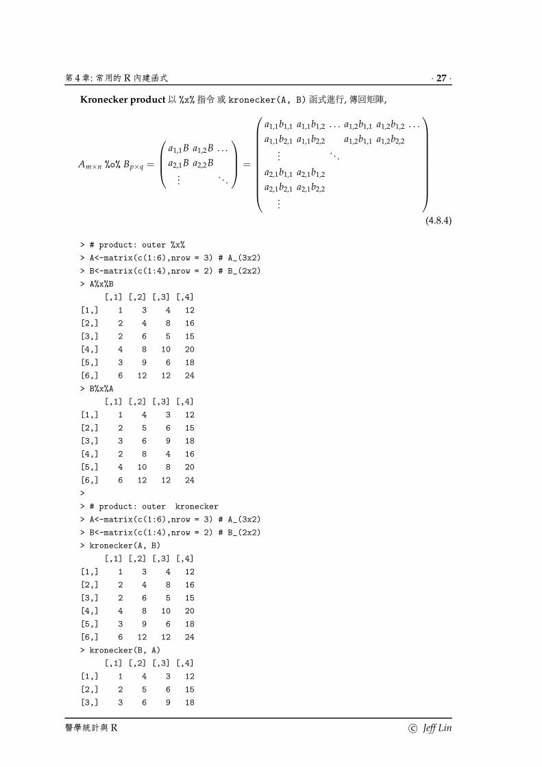
Kronecker product 以 %x% 指令 或 kronecker(A, B) 函式進行, 傳回矩陣,
Am×n %o% Bp×q =
a1,1B a1,2B . . .
a2,1B a2,2B...
. . .
=
a1,1b1,1 a1,1b1,2 . . . a1,2b1,1 a1,2b1,2 . . .
a1,1b2,1 a1,1b2,2 a1,2b1,1 a1,2b2,2
.... . .
a2,1b1,1 a2,1b1,2
a2,1b2,1 a2,1b2,2
...
(4.8.4)
> # product: outer %x%
> A<-matrix(c(1:6),nrow = 3) # A_(3x2)
> B<-matrix(c(1:4),nrow = 2) # B_(2x2)
> A%x%B
[,1] [,2] [,3] [,4]
[1,] 1 3 4 12
[2,] 2 4 8 16
[3,] 2 6 5 15
[4,] 4 8 10 20
[5,] 3 9 6 18
[6,] 6 12 12 24
> B%x%A
[,1] [,2] [,3] [,4]
[1,] 1 4 3 12
[2,] 2 5 6 15
[3,] 3 6 9 18
[4,] 2 8 4 16
[5,] 4 10 8 20
[6,] 6 12 12 24
>
> # product: outer kronecker
> A<-matrix(c(1:6),nrow = 3) # A_(3x2)
> B<-matrix(c(1:4),nrow = 2) # B_(2x2)
> kronecker(A, B)
[,1] [,2] [,3] [,4]
[1,] 1 3 4 12
[2,] 2 4 8 16
[3,] 2 6 5 15
[4,] 4 8 10 20
[5,] 3 9 6 18
[6,] 6 12 12 24
> kronecker(B, A)
[,1] [,2] [,3] [,4]
[1,] 1 4 3 12
[2,] 2 5 6 15
[3,] 3 6 9 18
醫學統計與 R c© Jeff Lin

· 28 · 4.8 線性代數函式
[4,] 2 8 4 16
[5,] 4 10 8 20
[6,] 6 12 12 24
函數 crossprod() 可以完成 “矢積, 叉乘積”(crossproduct) 運算, 也就是說 crossprod(X,
Y) 和 t(X) %*% Y 一樣, 但是在運算上更有效率. 如果 crossprod()第二個引數省略了, 它將和第
一個參數一樣.
> # product: crossproduct()
> A<-matrix(c(1:6),nrow = 3) # A_(3x2)
> B<-matrix(c(1:6),nrow = 3) # B_(3x2)
> crossprod(A,B)
[,1] [,2]
[1,] 14 32
[2,] 32 77
> t(A) %*% B
[,1] [,2]
[1,] 14 32
[2,] 32 77
矩陣 Am×n 的次方 (power), Ak, 可以直接使用 ^ (注意: 只有方陣 (square matrix) 才能求出其
次方).
> # product: power "^"
> A<-matrix(c(1:9),nrow = 3) # square matrix A_(3x3)
> A^3
[,1] [,2] [,3]
[1,] 1 64 343
[2,] 8 125 512
[3,] 27 216 729
4.8.3 矩陣行列式值
假設 AAA 是一個 “方塊矩陣” (方陣, square matrix), 則其 行列式值 (determinant) 為
det(A) = |A| (4.8.5)
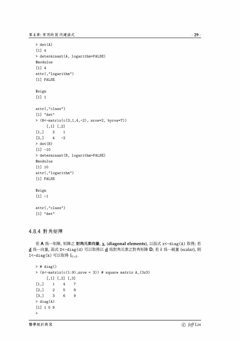
R 有 det() 與 determinant() 函式, det(A) 回傳行列式值, determinant(A, logarithm =
TRUE) 回傳一個列表物件, 包含 modulus (= log(|determinant|))與 sign(determinant).
> # det()
> (A<-matrix(c(1,2,3, 2,3,4, 3,4,1), nrow=3, byrow=T))
[,1] [,2] [,3]
[1,] 1 2 3
[2,] 2 3 4
[3,] 3 4 1
c© Jeff Lin 醫學統計與 R
第 4 章: 常用的 R 內建函式 · 29 ·
> det(A)
[1] 4
> determinant(A, logarithm=FALSE)
$modulus
[1] 4
attr(,"logarithm")
[1] FALSE
$sign
[1] 1
attr(,"class")
[1] "det"
> (B<-matrix(c(3,1,4,-2), nrow=2, byrow=T))
[,1] [,2]
[1,] 3 1
[2,] 4 -2
> det(B)
[1] -10
> determinant(B, logarithm=FALSE)
$modulus
[1] 10
attr(,"logarithm")
[1] FALSE
$sign
[1] -1
attr(,"class")
[1] "det"
4.8.4 對角矩陣
若 AAA 為一矩陣, 矩陣之 對角元素向量, x, (diagonal elements), 以函式 x<-diag(A) 取得; 若
d 為一向量, 函式 D<-diag(d) 可以取得以 d 為對角元素之對角矩陣 DDD; 若 k 為一純量 (scalar), 則
I<-diag(k) 可以取得 Ik×k.
> # diag()
> (A<-matrix(c(1:9),nrow = 3)) # square matrix A_(3x3)
[,1] [,2] [,3]
[1,] 1 4 7
[2,] 2 5 8
[3,] 3 6 9
> diag(A)
[1] 1 5 9
>
醫學統計與 R c© Jeff Lin

· 30 · 4.8 線性代數函式
> diag(rep(2,3))
[,1] [,2] [,3]
[1,] 2 0 0
[2,] 0 2 0
[3,] 0 0 2
> diag(3)
[,1] [,2] [,3]
[1,] 1 0 0
[2,] 0 1 0
[3,] 0 0 1
>
> (B<-matrix(c(1:6),nrow = 3)) # B_(3x2)
[,1] [,2]
[1,] 1 4
[2,] 2 5
[3,] 3 6
> diag(B)
[1] 1 5
>
> (B<-matrix(c(1:6),nrow = 2)) # B_(2x3)
[,1] [,2] [,3]
[1,] 1 3 5
[2,] 2 4 6
> diag(B)
[1] 1 4
4.8.5 反矩陣與線性方程式
反矩陣 (matrix inverse) 與解線性方程式, 假設 AAA 是一個方塊矩陣 (square matrix), 則其反矩
陣可用 solve(A)求出. 解線性方程式 b = AAAx, (b = A %*% x), 已知 AAA與 b, 欲求 x 的解,須利用反
矩陣概念, 在 R 可以用 x<-solve(A, b). 若要計算 xTAAA−1x二次型式的結果, 以 x %*% solve(A,
x)較有效率.
b = AAAx (4.8.6)
x = AAA−1b (4.8.7)
x = solve(AAA) %*% b (4.8.8)
x = solve(AAA, b) (4.8.9)
考慮以下線性方程式
b1 + 2b2 + 3b3 = 3
2b1 + 3b2 + 4b3 = 0
3b1 + 4b2 + b3 = 1
(4.8.10)
c© Jeff Lin 醫學統計與 R

第 4 章: 常用的 R 內建函式 · 31 ·
> # inverse, linear equation
> (A<-matrix(c(1,2,3, 2,3,4, 3,4,1), nrow = 3, byrow = T))
[,1] [,2] [,3]
[1,] 1 2 3
[2,] 2 3 4
[3,] 3 4 1
> (b<-c(3,0,1))
[1] 3 0 1
> solve(A)
[,1] [,2] [,3]
[1,] -3.25 2.5 -0.25
[2,] 2.50 -2.0 0.50
[3,] -0.25 0.5 -0.25
> round(solve(A)%*%A,2)
[,1] [,2] [,3]
[1,] 1 0 0
[2,] 0 1 0
[3,] 0 0 1
> x<-solve(A,b)
> A%*%x
[,1]
[1,] 2.99999999999999820000
[2,] -0.00000000000000177636
[3,] 1.00000000000000000000
>
4.8.6 特徵值和特徵向量
函式 EV<-eigen(Sm)用來計算矩陣 Sm 的 “特徵值” 和 “特徵向量” (eigenvalues and eigen-
vectors). 這個函式傳回一個含有兩個成分的列表, 分別是 EV$val 特徵值向量 和 EV$vec 特徵向量
組成的矩陣. prod(eigen(X)$valves)計算 XXX行列式的絕對值.
> # eigen valves and vectors
> (A<-matrix(c(1,2,3, 2,3,4, 3,4,1), nrow = 3, byrow = T))
[,1] [,2] [,3]
[1,] 1 2 3
[2,] 2 3 4
[3,] 3 4 1
> A.eig<-eigen(A)
> A.eig$values
[1] 7.862717 -0.190368 -2.672349
> A.eig$vectors
[,1] [,2] [,3]
[1,] -0.452500 0.781340 -0.429827
[2,] -0.670108 -0.615944 -0.414208
[3,] -0.588387 0.100601 0.802297
醫學統計與 R c© Jeff Lin

· 32 · 4.8 線性代數函式
> # determinant
> prod(eigen(A)$valves)
[1] 1
> det(A)
[1] 4
4.8.7 矩陣的奇異值分解
矩陣的奇異值分解 (SVD, Singular Value Decomposition) 是指
XXX = UUU %*% DDD %*% VVVT = UUUDDDVVVT (4.8.11)
使用函式 svd(X) 對 XXX進行奇異值分解. 這包括一個和 XXX 列空間 (row)一致的正交列 UUU 的矩陣,
一個和 XXX 行 (欄, column) 空間一致的正交列 VVV 的矩陣, 以及一個僅具正值之元素 DDD 的對角矩陣, 如
X = U %*% D %*% t(V). DDD 實際上以對角元素向量的形式傳回. svd(X) 的結果是由 d, u 和 v
構成的一個列表. 如果 XXX 是一個方塊矩陣, absdetM<-prod(svd(X)$d)計算XXX行列式的絕對值. 矩
陣主對角線元素和 (trace), 相當於特徵值和, 可以利用 DDD 得到.
> # SVD
> (A<-matrix(c(1,2,3, 2,3,4, 3,4,1), nrow = 3, byrow = T))
[,1] [,2] [,3]
[1,] 1 2 3
[2,] 2 3 4
[3,] 3 4 1
> b.svd<-svd(A)
> b.svd$d
[1] 7.862717 2.672349 0.190368
> b.svd$u
[,1] [,2] [,3]
[1,] -0.452500 -0.429827 -0.781340
[2,] -0.670108 -0.414208 0.615944
[3,] -0.588387 0.802297 -0.100601
> b.svd$v
[,1] [,2] [,3]
[1,] -0.452500 0.429827 0.781340
[2,] -0.670108 0.414208 -0.615944
[3,] -0.588387 -0.802297 0.100601
>
> # determinant
> det (A)
[1] 4
> prod(svd(A)$d)
[1] 4
c© Jeff Lin 醫學統計與 R

第 4 章: 常用的 R 內建函式 · 33 ·
4.8.8 矩陣的 QR 與 Cholski 分解
矩陣除了奇異值分解分解外, 尚有 QR與 Cholski 分解, QR 分解是將 XXX 矩陣分解成一個 QQQ 矩陣
與 RRR 矩陣的乘積, XXX = QQQRRR, 其中 RRR 是上三角矩陣, Q 是直交矩陣 (orthogonal matrix), QQQTQQQ = III.
或者QQQ 是擁有互相垂直的單位行 (欄, column) 向量之矩陣,而且此單位行向量之集合, 形成矩陣 XXX 之
行向量空間 (欄, column space). QR 分解在計算矩陣行列式值 (determinant)較 eigen()要有效
率. B.qr.list<-qr(X) 可進行 QR 分解, 回傳一陣列 B.list, 其中的矩陣 B.list$qr 將 QQQ 矩陣
與 RRR 矩陣放在一起. qr.X(B.qr.list), qr.Q(B.qr.list). qr.R(B.qr.list) 可以還原 XXX, 以
及 QQQ與 RRR.
# QR
> (X<-matrix(c(1,2,3, 2,3,4, 3,4,1), nrow = 3, byrow = T))
[,1] [,2] [,3]
[1,] 1 2 3
[2,] 2 3 4
[3,] 3 4 1
> (Xqr<-qr(X))
$qr
[,1] [,2] [,3]
[1,] -3.741657 -5.345225 -3.74166
[2,] 0.534522 0.654654 3.05505
[3,] 0.801784 0.988693 -1.63299
$rank
[1] 3
$qraux
[1] 1.26726 1.14995 1.63299
$pivot
[1] 1 2 3
attr(,"class")
[1] "qr"
> (X.back<-qr.X(Xqr))
[,1] [,2] [,3]
[1,] 1 2 3
[2,] 2 3 4
[3,] 3 4 1
> (R.back<-qr.R(Xqr))
[,1] [,2] [,3]
[1,] -3.74166 -5.345225 -3.74166
[2,] 0.00000 0.654654 3.05505
[3,] 0.00000 0.000000 -1.63299
> (Q.back<-qr.Q(Xqr))
[,1] [,2] [,3]
[1,] -0.267261 0.872872 0.408248
醫學統計與 R c© Jeff Lin

· 34 · 4.8 線性代數函式
[2,] -0.534522 0.218218 -0.816497
[3,] -0.801784 -0.436436 0.408248
> Q.back%*%R.back
[,1] [,2] [,3]
[1,] 1 2 3
[2,] 2 3 4
[3,] 3 4 1
當矩陣 XXX 是對稱正向 (symmetric positive definite) 矩陣, 利用 Cholski 分解, 則 XXX 可分
解成上三角矩陣 RRR, 與下三角矩陣 RRRT 的乘積, 即 XXX = RRRTRRR, 其中上三角矩陣 RRR 主對角上的元素
RRR1,1 =√
XXX1,1. RRRi,i =√
Xi,i − ∑k RRR2k,i, k = 1, . . . , i − 1. 函式 chol(X) 執行 Cholski 分解, 若矩
陣 XXX 不是對稱正向矩陣, 則函式無法執行.
> # Choleski Decomposition
> (X<-matrix(c(2,-1,-3, -1,2,4, -3,4,9), nrow = 3, byrow = T))
[,1] [,2] [,3]
[1,] 2 -1 -3
[2,] -1 2 4
[3,] -3 4 9
> # (X.chol<-chol(X, pivot = TRUE))
> (X.chol<-chol(X))
[,1] [,2] [,3]
[1,] 1.41421 -0.707107 -2.12132
[2,] 0.00000 1.224745 2.04124
[3,] 0.00000 0.000000 0.57735
> t(X.chol)%*%X.chol
[,1] [,2] [,3]
[1,] 2 -1 -3
[2,] -1 2 4
[3,] -3 4 9
> crossprod(X.chol)
[,1] [,2] [,3]
[1,] 2 -1 -3
[2,] -1 2 4
[3,] -3 4 9
c© Jeff Lin 醫學統計與 R

第 4 章: 常用的 R 內建函式 · 35 ·
4.9 列聯表函式 Cross-Tabulation Function
在 R 中,一些函式用來製造或操作列聯表 ( contingency table), 如 table(), ftable(), xtabs(),
margin.table(), prop.table()等.
table() 函式, 從任何向量, 創造列聯表, 回傳一個 “列聯表. “ contingency table ”, 是一個
R 物件類別 (class) 為 "table" 之物件. as.table()與 is.table() 用來強制形成列聯表物件或
查看列聯表物件.
> # table()
> xvec<-c(rep(0,5), rep(1,7), rep(2,6), rep(3,6))
> yvec<-rep(c(1,0), 12)
> zvec<-rep(c(1,2), times = c(12,12))
> xyz.data<-data.frame(xdat = xvec, ydat = yvec, zdat = zvec)
> xyz.data
xdat ydat zdat
1 0 1 1
2 0 0 1
3 0 1 1
4 0 0 1
5 0 1 1
6 1 0 1
7 1 1 1
8 1 0 1
9 1 1 1
10 1 0 1
11 1 1 1
12 1 0 1
13 2 1 2
14 2 0 2
15 2 1 2
16 2 0 2
17 2 1 2
18 2 0 2
19 3 1 2
20 3 0 2
21 3 1 2
22 3 0 2
23 3 1 2
24 3 0 2
> attach(xyz.data)
>
> xy.tab<-table(xdat, ydat)
> xy.tab
ydat
xdat 0 1
醫學統計與 R c© Jeff Lin

· 36 · 4.9 列聯表函式
0 2 3
1 4 3
2 3 3
3 3 3
> xyz.tab<-table(xdat, ydat, zdat)
> xyz.tab
, , zdat = 1
ydat
xdat 0 1
0 2 3
1 4 3
2 0 0
3 0 0
, , zdat = 2
ydat
xdat 0 1
0 0 0
1 0 0
2 3 3
3 3 3
ftable() 函式, 從任何向量, 創造一個 “扁平” (flat) 列聯表, 扁平列聯表是一個 "ftalbe" 類
別 (class) 矩陣物件, 其中變數 (欄位) 為分類因子變數, 令外再加上各組頻率數目, 每一列 (row) 代表
每一種分類階層 (level), 列印較 table() 好看. read.ftable() 與 write.ftable() 用來讀寫
"ftalbe"類別矩陣物件.
> # ftable()
> xy.ftab<-ftable(xdat, ydat)
> xy.ftab
ydat 0 1
xdat
0 2 3
1 4 3
2 3 3
3 3 3
> xyz.ftab<-ftable(xdat, ydat, zdat)
> xyz.ftab
zdat 1 2
xdat ydat
0 0 2 0
1 3 0
1 0 4 0
1 3 0
2 0 0 3
c© Jeff Lin 醫學統計與 R

第 4 章: 常用的 R 內建函式 · 37 ·
1 0 3
3 0 0 3
1 0 3
xtabs()函式, 從資料框架中, 利用統計模型公式 (model formula) 創造一個列聯表; as.data.frame()
函式是 xtabs() 反函式, 從列聯表物件創造一個資料框架.
> # xtabs()
> xy.xtabs<-xtabs(~xdat+ydat)
> xy.xtabs
ydat
xdat 0 1
0 2 3
1 4 3
2 3 3
3 3 3
> xyz.xtabs<-xtabs(~xdat+ydat+zdat)
> xyz.xtabs
, , zdat = 1
ydat
xdat 0 1
0 2 3
1 4 3
2 0 0
3 0 0
, , zdat = 2
ydat
xdat 0 1
0 0 0
1 0 0
2 3 3
3 3 3
> # as.data.frame
> xy.as<-as.data.frame(xy.xtabs)
> xy.as
xdat ydat Freq
1 0 0 2
2 1 0 4
3 2 0 3
4 3 0 3
5 0 1 3
6 1 1 3
7 2 1 3
醫學統計與 R c© Jeff Lin

· 38 · 4.9 列聯表函式
8 3 1 3
> xyz.as<-as.data.frame(xyz.xtabs)
> xyz.as
xdat ydat zdat Freq
1 0 0 1 2
2 1 0 1 4
3 2 0 1 0
4 3 0 1 0
5 0 1 1 3
6 1 1 1 3
7 2 1 1 0
8 3 1 1 0
9 0 0 2 0
10 1 0 2 0
11 2 0 2 3
12 3 0 2 3
13 0 1 2 0
14 1 1 2 0
15 2 1 2 3
16 3 1 2 3
margin.table(x, margin = NULL) 函式從陣列型式之列聯表物件, 計算邊際總合, margin
下標 1 為列 (row), 依此列推. prop.table(x, margin = NULL) 函式從陣列型式之列聯表物件,
計算列聯表內的相對頻率, 是 sweep(x, margin, margin.table(x, margin), "/") 的簡化.
> # margin.table(), prop.table()
> margin.table(xy.tab, margin = 1)
xdat
0 1 2 3
5 7 6 6
> prop.table(xy.tab, margin = 1)
ydat
xdat 0 1
0 0.4000000 0.6000000
1 0.5714286 0.4285714
2 0.5000000 0.5000000
3 0.5000000 0.5000000
>
> margin.table(xyz.tab, margin = 2)
ydat
0 1
12 12
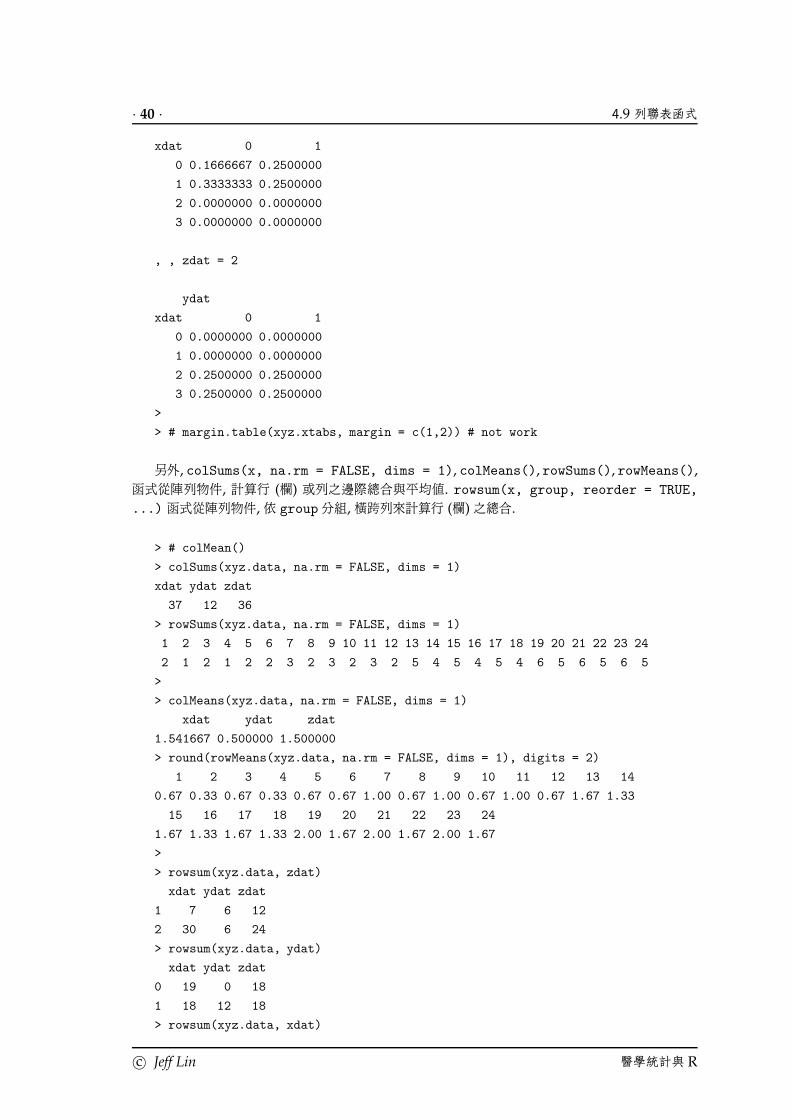
> prop.table(xyz.tab, margin = 2)
, , zdat = 1
ydat
xdat 0 1
c© Jeff Lin 醫學統計與 R

第 4 章: 常用的 R 內建函式 · 39 ·
0 0.1666667 0.2500000
1 0.3333333 0.2500000
2 0.0000000 0.0000000
3 0.0000000 0.0000000
, , zdat = 2
ydat
xdat 0 1
0 0.0000000 0.0000000
1 0.0000000 0.0000000
2 0.2500000 0.2500000
3 0.2500000 0.2500000
>
> margin.table(xyz.tab, margin = c(1,2))
ydat
xdat 0 1
0 2 3
1 4 3
2 3 3
3 3 3
>
> # margin.table(xy.ftab, margin = 1) # not work
> # margin.table(xyz.ftab, margin = 2) # not work
> # margin.table(xyz.ftab, margin = c(1,2)) # not work
>
> margin.table(xy.xtabs, margin = 1)
xdat
0 1 2 3
5 7 6 6
> prop.table(xy.xtabs, margin = 1)
ydat
xdat 0 1
0 0.4000000 0.6000000
1 0.5714286 0.4285714
2 0.5000000 0.5000000
3 0.5000000 0.5000000
>
> margin.table(xyz.xtabs, margin = 2)
ydat
0 1
12 12
> prop.table(xyz.xtabs, margin = 2)
, , zdat = 1
ydat
醫學統計與 R c© Jeff Lin
· 40 · 4.9 列聯表函式
xdat 0 1
0 0.1666667 0.2500000
1 0.3333333 0.2500000
2 0.0000000 0.0000000
3 0.0000000 0.0000000
, , zdat = 2
ydat
xdat 0 1
0 0.0000000 0.0000000
1 0.0000000 0.0000000
2 0.2500000 0.2500000
3 0.2500000 0.2500000
>
> # margin.table(xyz.xtabs, margin = c(1,2)) # not work
另外, colSums(x, na.rm = FALSE, dims = 1), colMeans(), rowSums(), rowMeans(),
函式從陣列物件, 計算行 (欄) 或列之邊際總合與平均值. rowsum(x, group, reorder = TRUE,
...) 函式從陣列物件, 依 group 分組, 橫跨列來計算行 (欄) 之總合.
> # colMean()
> colSums(xyz.data, na.rm = FALSE, dims = 1)
xdat ydat zdat
37 12 36
> rowSums(xyz.data, na.rm = FALSE, dims = 1)
1 2 3 4 5 6 7 8 9 10 11 12 13 14 15 16 17 18 19 20 21 22 23 24
2 1 2 1 2 2 3 2 3 2 3 2 5 4 5 4 5 4 6 5 6 5 6 5
>
> colMeans(xyz.data, na.rm = FALSE, dims = 1)
xdat ydat zdat
1.541667 0.500000 1.500000
> round(rowMeans(xyz.data, na.rm = FALSE, dims = 1), digits = 2)
1 2 3 4 5 6 7 8 9 10 11 12 13 14
0.67 0.33 0.67 0.33 0.67 0.67 1.00 0.67 1.00 0.67 1.00 0.67 1.67 1.33
15 16 17 18 19 20 21 22 23 24
1.67 1.33 1.67 1.33 2.00 1.67 2.00 1.67 2.00 1.67
>
> rowsum(xyz.data, zdat)
xdat ydat zdat
1 7 6 12
2 30 6 24
> rowsum(xyz.data, ydat)
xdat ydat zdat
0 19 0 18
1 18 12 18
> rowsum(xyz.data, xdat)
c© Jeff Lin 醫學統計與 R

第 4 章: 常用的 R 內建函式 · 41 ·
xdat ydat zdat
0 0 3 5
1 7 3 7
2 12 3 12
3 18 3 12
4.10 apply(), lapply(), sapply(), mapply(), tapply(),
by(), sweep(), aggregate() · · · 等函式
在 R 中, 許多函式利用向量做運算, 但更多時候, 必須對許多的向量使用同一函式做運算, 如對資
料框架內的每一變數 (行向量), 計算平均值與變異數. 有時候, 針對一變數, 更據不同的組別, 分別使
用同一函式做運算, 如根據不同治療組別, 分別計算血壓的計算平均值與變異數. 在上述的情形, 常常
須用到迴圈, R 迴圈的執行非常無效率, 應儘量避免,. 因此, 在 R 有些函式如 apply(), lapply(),
sapply(), replicate(), tapply(), mapply()等, 可以更有效率的執行類似迴圈的函式指令.
4.10.1 apply() 函式
apply(X, MARGIN, FUN, ...) 對一陣列 X 的邊際 (margins of an array) 執行同一函式做
運算, 並回傳一向量, 陣列或列表. 其中引數 x 為所要執行之陣列物件, MARGIN 為陣列的邊際維度序號,
FUN 為執行同一函式的名稱. 若 X 為矩陣或資料框架, apply() 會將該矩陣或資料框架轉換成 2-維度
陣列. MARGIN = 1 會對陣列物件 x 的第 1 的維度執行函式, (如矩陣或資料框架的每一列 (row)) 做運
算, MARGIN = 2 會對陣列物件 x 的第 2 的維度執行函式, (如矩陣或資料框架的每一行 (欄, column))
做運算,等等.
> # apply() and array
> a<-1:48
> b.arr<-array(a, dim=c(4,3,4), dimnames=c("x", "y", "z"))
> b.arr
, , 1
[,1] [,2] [,3]
[1,] 1 5 9
[2,] 2 6 10
[3,] 3 7 11
[4,] 4 8 12
, , 2
[,1] [,2] [,3]
[1,] 13 17 21
[2,] 14 18 22
[3,] 15 19 23
醫學統計與 R c© Jeff Lin

· 42 · 4.10 apply() · · · 等函式
[4,] 16 20 24
, , 3
[,1] [,2] [,3]
[1,] 25 29 33
[2,] 26 30 34
[3,] 27 31 35
[4,] 28 32 36
, , 4
[,1] [,2] [,3]
[1,] 37 41 45
[2,] 38 42 46
[3,] 39 43 47
[4,] 40 44 48
> b.arr[1, , ]
[,1] [,2] [,3] [,4]
[1,] 1 13 25 37
[2,] 5 17 29 41
[3,] 9 21 33 45
> mean(b.arr[1, , ])
[1] 23
>
> b.arr[ , 2, ]
[,1] [,2] [,3] [,4]
[1,] 5 17 29 41
[2,] 6 18 30 42
[3,] 7 19 31 43
[4,] 8 20 32 44
> mean(b.arr[ , 2, ])
[1] 24.5
>
> b.arr[ , ,3]
[,1] [,2] [,3]
[1,] 25 29 33
[2,] 26 30 34
[3,] 27 31 35
[4,] 28 32 36
> mean(b.arr[ , ,3])
[1] 30.5
>
> # matrix, data
> a<-1:48
> b.data<-as.data.frame(matrix(a, nrow = 12, byrow = T))
c© Jeff Lin 醫學統計與 R

第 4 章: 常用的 R 內建函式 · 43 ·
> b.data
V1 V2 V3 V4
1 1 2 3 4
2 5 6 7 8
3 9 10 11 12
4 13 14 15 16
5 17 18 19 20
6 21 22 23 24
7 25 26 27 28
8 29 30 31 32
9 33 34 35 36
10 37 38 39 40
11 41 42 43 44
12 45 46 47 48
>
> # apply()
> apply(b.arr, 1, mean)
[1] 23 24 25 26
> apply(b.arr, 2, mean)
[1] 20.5 24.5 28.5
> apply(b.arr, 3, mean)
[1] 6.5 18.5 30.5 42.5
>
> apply(b.data, 1, mean)
1 2 3 4 5 6 7 8 9 10 11 12
2.5 6.5 10.5 14.5 18.5 22.5 26.5 30.5 34.5 38.5 42.5 46.5
> apply(b.data, 2, mean)
V1 V2 V3 V4
23 24 25 26
4.10.2 lapply() 與 sapply() 函式
lapply(X, , FUN, ...) 對一列表的每一成分 (component), 執行同一函式, 回傳一個列表
物件, 且此回傳的列表物件長度與原有 X 長度相同. sapply(X, FUN, ..., simplify = TRUE,
USE.NAMES = TRUE)是較容易使用的 lapply()函式, 且回傳一向量或矩陣. sapply(X.data)對
資料框架 (列表物件) X.data 執行同一函式, 是指對每一個變數 (欄), 做運算.
> # lapply(), sallpy(), replicate()
> # list + lapply()
> c.list<-list(a = 1:20,
+ beta = exp(-2:2),
+ logic = c(TRUE,FALSE,FALSE,TRUE,FALSE))
> lapply(c.list, mean)
$a
[1] 10.5
醫學統計與 R c© Jeff Lin

· 44 · 4.10 apply() · · · 等函式
$beta
[1] 2.322111
$logic
[1] 0.4
> # list + sapply()
> sapply(c.list, mean, simplify = FALSE)
$a
[1] 10.5
$beta
[1] 2.322111
$logic
[1] 0.4
> sapply(c.list, mean, simplify = TRUE)
a beta logic
10.500000 2.322111 0.400000
>
> sapply(b.data, mean) # for each variable in a data.frame
V1 V2 V3 V4
23 24 25 26
4.10.3 replicate() 函式
replicate(n, expr, simplify = TRUE) 如同 sapply() 的包裝封套, 可以重覆執行同一
運算式 (expr),通常是執行產生隨機變數.
> # replicate
> replicate(5, rexp(10))
[,1] [,2] [,3] [,4] [,5]
[1,] 0.002377610 1.12608402 1.3655184 0.770839129 1.2173416
[2,] 0.095294966 1.07961521 0.7859411 0.126137957 1.1453436
[3,] 0.292917136 0.01132655 0.4803611 3.272213980 0.5079139
[4,] 0.194720482 0.12017418 0.3639454 0.001253859 1.4902494
[5,] 0.053378940 0.10680672 1.4500199 0.031822894 0.3266150
[6,] 0.028073654 0.49771918 2.0123197 0.794271854 0.6262215
[7,] 0.151922586 0.53818551 0.5569553 0.619600469 1.1510464
[8,] 0.267240588 3.29991750 0.2520244 0.097163025 0.9194827
[9,] 0.152619028 0.34104853 1.4342287 2.080907619 1.4058583
[10,] 0.010633701 3.25183414 1.1823071 0.242085239 1.7422518
> replicate(5, mean(rexp(10)))
[1] 0.6962537 0.8582474 0.7792168 1.1299690 0.7481463
c© Jeff Lin 醫學統計與 R

第 4 章: 常用的 R 內建函式 · 45 ·
4.10.4 tapply() 函式
tapply(X, INDEX, FUN = NULL, ..., simplify = TRUE)對一參差不齊的陣列, 更據不
同的組別指標值, 分別使用同一函式做運算, 引數 X 通常是一個向量 (可以為一陣列), INDEX通常是一
個組別因子陣列 (或向量),長度與 X 相同.
> # tapply()
> x.vec<-1:12
> y.group<-c(1,2,1,1,2,2,1,1,1,1,1,1)
> cbind(x.vec, y.group)
x.vec y.group
[1,] 1 1
[2,] 2 2
[3,] 3 1
[4,] 4 1
[5,] 5 2
[6,] 6 2
[7,] 7 1
[8,] 8 1
[9,] 9 1
[10,] 10 1
[11,] 11 1
[12,] 12 1
> tapply(x.vec, y.group, mean)
1 2
7.222222 4.333333
>
> # data + tapply()
> b.data<-as.data.frame(matrix(c(1:48), nrow = 12, byrow = T))
> b.data<-transform(b.data, sex = rep(c(1:2),6), race = rep(c(1:3),4))
> b.data
V1 V2 V3 V4 sex race
1 1 2 3 4 1 1
2 5 6 7 8 2 2
3 9 10 11 12 1 3
4 13 14 15 16 2 1
5 17 18 19 20 1 2
6 21 22 23 24 2 3
7 25 26 27 28 1 1
8 29 30 31 32 2 2
9 33 34 35 36 1 3
10 37 38 39 40 2 1
11 41 42 43 44 1 2
12 45 46 47 48 2 3
> sapply(b.data, tapply, b.data$sex, mean) # not easy to understand
V1 V2 V3 V4 sex race
1 21 22 23 24 1 2
醫學統計與 R c© Jeff Lin

· 46 · 4.10 apply() · · · 等函式
2 25 26 27 28 2 2
4.10.5 mapply() 與 Vectorize() 函式
mapply(FUN, ARG1 = arg1, ARG2 = arg2, ..., MoreArgs = NULL, SIMPLIFY = TRUE,
USE.NAMES = TRUE) 是 sapply() 的多變量型式, 函式 FUN() 本身含有引數, 如 FUN(ARG1 =
arg1, ARG2 = arg2, ..., mapply()執行 FUN函式時, 使用 ARG1 = arg1的第 1 元素, ARG2 =
arg2 的第 1 元素, · · · ,等等, MoreArgs = list(), MoreArgs = 需要用列表物件, 來執行 FUN 函
式, 引數可以循環使用. mapply()回傳一向量, 矩陣或陣列表. Vectorize(FUN, vectorize.args
= arg.names, SIMPLIFY = TRUE, USE.NAMES = TRUE) 是 mapply() 的的包裝封套, 回傳一
新函式, 有如呼叫 mapply() 函式.
> ######
> # mapply()
> mapply(rep, 1:3, 3:1)
[[1]]
[1] 1 1 1
[[2]]
[1] 2 2
[[3]]
[1] 3
> mapply(rep, times = 1:3, x = 3:1)
[[1]]
[1] 3
[[2]]
[1] 2 2
[[3]]
[1] 1 1 1
> mapply(rep, times = 1:3, MoreArgs = list(x = 7))
[[1]]
[1] 7
[[2]]
[1] 7 7
[[3]]
[1] 7 7 7
>
> # Vectorize()
> vrep<-Vectorize(rep)
c© Jeff Lin 醫學統計與 R

第 4 章: 常用的 R 內建函式 · 47 ·
> vrep(1:3, 3:1)
[[1]]
[1] 1 1 1
[[2]]
[1] 2 2
[[3]]
[1] 3
> vrep(times = 1:3, x = 3:1)
[[1]]
[1] 3
[[2]]
[1] 2 2
[[3]]
[1] 1 1 1
> vrep<-Vectorize(rep, "times")
> vrep(times = 1:3, x = 7)
[[1]]
[1] 7
[[2]]
[1] 7 7
[[3]]
[1] 7 7 7
4.10.6 by() 函式
by()函式將資料框架依不同的組別因子, 計算統計量. 指令通常為 by(data, INDICES, FUN,
...), 其中 data為資料框架或矩陣, INDICES為組別因子向量,長度與資料框架變數長度 (nrows(data))
相同, FUN 是指所要計算的統計量.
> # by
> b.data<-as.data.frame(matrix(c(1:48), nrow = 12, byrow = T))
> b.data<-transform(b.data, sex = rep(c(1:2),6), race = rep(c(1:3),4))
> by(b.data, b.data$sex, mean)
b.data$sex: 1
V1 V2 V3 V4 sex race
21 22 23 24 1 2
----------------------------------------------------
b.data$sex: 2
醫學統計與 R c© Jeff Lin

· 48 · 4.10 apply() · · · 等函式
V1 V2 V3 V4 sex race
25 26 27 28 2 2
> #
> sapply(b.data, tapply, b.data$sex, mean) # not easy to understand
V1 V2 V3 V4 sex race
1 21 22 23 24 1 2
2 25 26 27 28 2 2
4.10.7 sweep() 函式
sweep(x, MARGIN, STATS, FUN = "-", ...) 對一輸入之陣列 (array) X之邊際維度 (MAR-
GIN), 對一統計量 (STATS, summary statistic), 進行某一特定運算 (FUN = ”-”), 此特定運算 (如
−)須加用雙引號, sweep()通常與 apply() 並用.
> help(sweep)
> # sweep()
> b.data<-as.data.frame(matrix(c(1:48), nrow = 12, byrow = T))
> b.mean<-apply(b.data,2,mean)
> sweep(b.data,2,b.mean)
V1 V2 V3 V4
1 -22 -22 -22 -22
2 -18 -18 -18 -18
3 -14 -14 -14 -14
4 -10 -10 -10 -10
5 -6 -6 -6 -6
6 -2 -2 -2 -2
7 2 2 2 2
8 6 6 6 6
9 10 10 10 10
10 14 14 14 14
11 18 18 18 18
12 22 22 22 22
4.10.8 aggregate() 函式
aggregate()函式將資料框架分成不同的組別, 分別計算統計量. 如 aggregate(X, by, FUN,
...), 其中 by 是長度與 X 變數相同的 (因子)變數用來分組, FUN 是指所要計算的統計量.
> # aggregate()
> b.data<-as.data.frame(matrix(c(1:48), nrow = 12, byrow = T))
> b.data<-transform(b.data, sex = rep(c(1:2),6), race = rep(c(1:3),4))
> aggregate(b.data, by = list(SEX = b.data$sex), mean)
SEX V1 V2 V3 V4 sex race
1 1 21 22 23 24 1 2
2 2 25 26 27 28 2 2
c© Jeff Lin 醫學統計與 R
第 4 章: 常用的 R 內建函式 · 49 ·
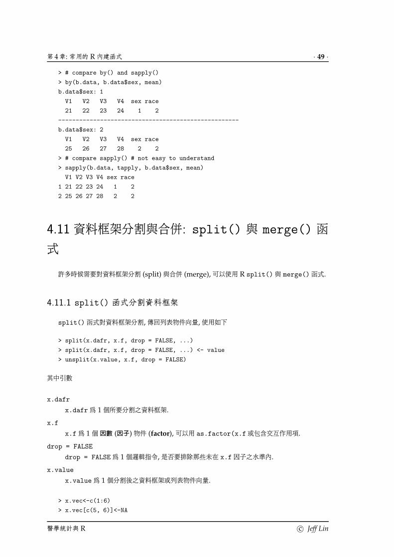
> # compare by() and sapply()
> by(b.data, b.data$sex, mean)
b.data$sex: 1
V1 V2 V3 V4 sex race
21 22 23 24 1 2
----------------------------------------------------
b.data$sex: 2
V1 V2 V3 V4 sex race
25 26 27 28 2 2
> # compare sapply() # not easy to understand
> sapply(b.data, tapply, b.data$sex, mean)
V1 V2 V3 V4 sex race
1 21 22 23 24 1 2
2 25 26 27 28 2 2
4.11 資料框架分割與合併: split() 與 merge() 函
式
許多時候需要對資料框架分割 (split)與合併 (merge), 可以使用 R split()與 merge() 函式.
4.11.1 split() 函式分割資料框架
split() 函式對資料框架分割, 傳回列表物件向量, 使用如下
> split(x.dafr, x.f, drop = FALSE, ...)
> split(x.dafr, x.f, drop = FALSE, ...) <- value
> unsplit(x.value, x.f, drop = FALSE)
其中引數
x.dafr
x.dafr 為 1 個所要分割之資料框架.
x.f
x.f 為 1 個 因數 (因子) 物件 (factor), 可以用 as.factor(x.f 或包含交互作用項.
drop = FALSE
drop = FALSE 為 1 個邏輯指令, 是否要排除那些未在 x.f 因子之水準內.
x.value
x.value 為 1 個分割後之資料框架或列表物件向量.
> x.vec<-c(1:6)
> x.vec[c(5, 6)]<-NA
醫學統計與 R c© Jeff Lin

· 50 · 4.11 資料框架分割與合併: split() 與 merge()
> x.f1<-rep(c(1,2),3)
> x.f2<-rep(c(1,2), each=3)
> x.f3<-rep(c(1,2,3), length.out=6)
> x.df<-data.frame(x.vec=x.vec, x.f1=x.f1, x.f2=x.f2, x.f3=x.f3)
> x.df
x.vec x.f1 x.f2 x.f3
1 1 1 1 1
2 2 2 1 2
3 3 1 1 3
4 4 2 2 1
5 NA 1 2 2
6 NA 2 2 3
> #
> x.split<-split(x.df, as.factor(x.f1))
> x.split
$‘1‘
x.vec x.f1 x.f2 x.f3
1 1 1 1 1
3 3 1 1 3
5 NA 1 2 2
$‘2‘
x.vec x.f1 x.f2 x.f3
2 2 2 1 2
4 4 2 2 1
6 NA 2 2 3
4.11.2 merge() 函式合併資料框架
merge(x.dafr, y.dafr, ...) 函式對資料框架 x.dafr, y.dafr 合併, 傳回資料框架物件,
使用如下
> merge(x, y, by = intersect(names(x), names(y)),
by.x = "by.x.name", by.y = "by.y.name",
all.x = all, all.y = all, all = FALSE,
sort = TRUE, suffixes = c(".x",".y"), ...)
其中引數
x.dafr, y.dafr
x.dafr, y.dafr 為所要合併之資料框架.
by, by.x="x.anme", by.y="y.name"
設定 x.dafr, y.dafr合併之資料框架中, 所依據之共同之變數欄位名稱 (common columns),
如 by.x="x.name", by.y=y.name".
c© Jeff Lin 醫學統計與 R

第 4 章: 常用的 R 內建函式 · 51 ·
all.x, all.y, all
all.x 為 1 個邏輯指令, 當all.x = TRUE 時, 在所要合併之資料框架 x.dafr, 若與資料框
架 y.dafr 沒有相配之 by.y 列位 (rows), 會附加在合併後之資料框架最後, 並設定在相對應
之 by.y變數為 NA. all.y 為 1 個邏輯指令, 作用與 all.x類似. all表示 all.x, all.y 有
相同之邏輯指令.
suffixes = c(".x",".y")
在 x.dafr, y.dafr 合併之資料框架中,非合併所依據之共同之變數的其餘變數欄位名稱,若有
仍有相同的變數欄位名稱, 則會附加文字在其餘仍有相同名稱變數欄位.
> # merge
> x.vec<-c(1:6)
> x.f1<-rep(c(1,2),3)
> x.f2<-rep(c(1,2), each=3)
> x.f3<-rep(c(1,2,3), length.out=6)
> x.df<-data.frame(x.vec=x.vec, x.f1=x.f1, x.f2=x.f2, x.f3=x.f3)
> x.df
x.vec x.f1 x.f2 x.f3
1 1 1 1 1
2 2 2 1 2
3 3 1 1 3
4 4 2 2 1
5 5 1 2 2
6 6 2 2 3
> #
> y.vec<-c(3:8)
> x.f1<-rep(c(1,2),3)
> y.f2<-rep(c(1,2), each=3)
> y.f3<-rep(c(1,2,3,4), length.out=6)
> y.df<-data.frame(y.vec=y.vec, x.f1=x.f1, y.f2=y.f2, y.f3=y.f3)
> y.df
y.vec x.f1 y.f2 y.f3
1 3 1 1 1
2 4 2 1 2
3 5 1 1 3
4 6 2 2 4
5 7 1 2 1
6 8 2 2 2
> #
> merge(x.df, y.df, by.x="x.vec", by.y="y.vec", sort=FALSE)
x.vec x.f1.x x.f2 x.f3 x.f1.y y.f2 y.f3
1 3 1 1 3 1 1 1
2 4 2 2 1 2 1 2
3 5 1 2 2 1 1 3
4 6 2 2 3 2 2 4
> merge(x.df, y.df, by.x="x.vec", by.y="y.vec", all=TRUE, sort=FALSE)
x.vec x.f1.x x.f2 x.f3 x.f1.y y.f2 y.f3
醫學統計與 R c© Jeff Lin

· 52 · 4.11 資料框架分割與合併: split() 與 merge()
1 3 1 1 3 1 1 1
2 4 2 2 1 2 1 2
3 5 1 2 2 1 1 3
4 6 2 2 3 2 2 4
5 1 1 1 1 NA NA NA
6 2 2 1 2 NA NA NA
7 7 NA NA NA 1 2 1
8 8 NA NA NA 2 2 2
> merge(y.df, x.df, by.x="y.vec", by.y="x.vec", all=TRUE, sort=TRUE)
y.vec x.f1.x y.f2 y.f3 x.f1.y x.f2 x.f3
1 1 NA NA NA 1 1 1
2 2 NA NA NA 2 1 2
3 3 1 1 1 1 1 3
4 4 2 1 2 2 2 1
5 5 1 1 3 1 2 2
6 6 2 2 4 2 2 3
7 7 1 2 1 NA NA NA
8 8 2 2 2 NA NA NA
> merge(x.df, y.df, by.x="x.vec", by.y="y.vec",
+ sort=FALSE, all=TRUE, suffixes = c(".X",".Y"))
x.vec x.f1.X x.f2 x.f3 x.f1.Y y.f2 y.f3
1 3 1 1 3 1 1 1
2 4 2 2 1 2 1 2
3 5 1 2 2 1 1 3
4 6 2 2 3 2 2 4
5 1 1 1 1 NA NA NA
6 2 2 1 2 NA NA NA
7 7 NA NA NA 1 2 1
8 8 NA NA NA 2 2 2
c© Jeff Lin 醫學統計與 R

第 4 章: 常用的 R 內建函式 · 53 ·
4.12 物件查看與強制轉換函式
R 的函式, is.object(), 如 is.na(), is.vector()等, 用來查看某一特定物件是否屬於某一
類別. as.object(), 如 as.vector(), as.matrix(()等, 用來某強制轉換一特定物件到所指定的
物件類別,見表 4.5, 詳見輔助文件.
表 4.5: 物件查看與強制轉換函式
物件查看函式 強制轉換函式
is.na() n/a
is.nan() n/a
is.null() as.null()
is.numeric() as.numeric()
is.integer() as.integer()
is.character() as.character()
is.logical() as.logical()
is.complex() as.complex()
is.vector() as.vector()
is.matrix() as.matrix()
is.array() as.array()
is.list() as.list()
is.data.frame() as.data.frame()
is.ordered() as.ordered()
is.table() as.table()
is.function() as.function()
> # is() and as()
> xvec<-1:12
> is.vector(xvec)
[1] TRUE
> is.character(xvec)
[1] FALSE
>
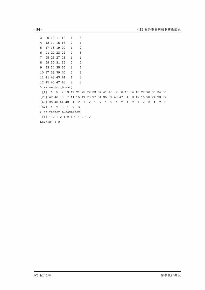
> b.data<-as.data.frame(matrix(c(1:48), nrow = 12, byrow = T))
> b.data<-transform(b.data, sex = rep(c(1:2),6), race = rep(c(1:3),4))
> is.matrix(b.data)
[1] FALSE
> b.mat<-as.matrix(b.data)
> b.mat
V1 V2 V3 V4 sex race
1 1 2 3 4 1 1
2 5 6 7 8 2 2
醫學統計與 R c© Jeff Lin
· 54 · 4.12 物件查看與強制轉換函式
3 9 10 11 12 1 3
4 13 14 15 16 2 1
5 17 18 19 20 1 2
6 21 22 23 24 2 3
7 25 26 27 28 1 1
8 29 30 31 32 2 2
9 33 34 35 36 1 3
10 37 38 39 40 2 1
11 41 42 43 44 1 2
12 45 46 47 48 2 3
> as.vector(b.mat)
[1] 1 5 9 13 17 21 25 29 33 37 41 45 2 6 10 14 18 22 26 30 34 38
[23] 42 46 3 7 11 15 19 23 27 31 35 39 43 47 4 8 12 16 20 24 28 32
[45] 36 40 44 48 1 2 1 2 1 2 1 2 1 2 1 2 1 2 3 1 2 3
[67] 1 2 3 1 2 3
> as.factor(b.data$sex)
[1] 1 2 1 2 1 2 1 2 1 2 1 2
Levels: 1 2
c© Jeff Lin 醫學統計與 R