CBinfer: Change-Based Inference for Convolutional NeuralNetworks on Video Data

Lukas CavigelliETH Zurich, Zurich, Switzerland

cavigelli@iis.ee.ethz.ch

Philippe DegenETH Zurich, Zurich, Switzerland

degenp@ee.ethz.ch

Luca BeniniETH Zurich, Zurich, Switzerland

benini@iis.ee.ethz.ch

ABSTRACTExtracting per-frame features using convolutional neural networksfor real-time processing of video data is currently mainly performedon powerful GPU-accelerated workstations and compute clusters.However, there are many applications such as smart surveillancecameras that require or would benefit from on-site processing. Tothis end, we propose and evaluate a novel algorithm for change-based evaluation of CNNs for video data recorded with a staticcamera setting, exploiting the spatio-temporal sparsity of pixelchanges. We achieve an average speed-up of 8.6× over a cuDNNbaseline on a realistic benchmark with a negligible accuracy loss ofless than 0.1% and no retraining of the network. The resulting en-ergy efficiency is 10× higher than that of per-frame evaluation andreaches an equivalent of 328GOp/s/W on the Tegra X1 platform.

1 INTRODUCTIONComputer vision (CV) technology has become a key ingredientfor automatized data analysis over a broad range of real-worldapplications: smart cameras for video surveillance, robotics, indus-trial quality assurance, medical diagnostics, and advanced driverassistance systems have recently become popular due the risingreliability of CV algorithms [15, 16, 37, 46]. This industry interesthas fostered the procedure of a wealth of research projects yieldinga fierce competition on many benchmarks datasets such as theImageNet/ILSVRC [13, 41], MS COCO [33], and Cityscapes [11]benchmarks, on which scientists from academia and big industryplayers evaluate their latest algorithms.

In recent years, the most competitive approaches to addressmany CV challenges have relied on machine learning with com-plex, multi-layered, trained feature extractors commonly referredto as deep learning [20, 28, 43]. The most frequently used flavorof deep learning techniques for CV are convolutional neural net-works (ConvNets, CNNs). Since their landslide success at the 2012ILSVRC competition over hand-crafted features, their accuracy hasfurther improved year-over-year even exceeding human perfor-mance on this complex dataset [21, 41]. CNNs keep on expandingto more areas of computer vision and data analytics in general[1, 16, 21, 34, 35, 45].

Unfortunately, the high accuracy of CNNs comes with a highcomputational cost, requiring powerful GPU servers to train thesenetworks for several weeks using hundreds of gigabytes of labeleddata. While this effort is very costly, it is a one-time endeavour andcan be done offline for many applications. However, the inferenceof state-of-the-art CNNs also requires several billions of multipli-cations and additions to classify even low resolution images bytoday’s standards [7]. While in some cases offloading to central-ized compute centers with powerful GPU servers is also possiblefor inference after deployment, it is extremely costly in terms of

compute infrastructure and energy. Furthermore, collecting largeamounts of data at a central site raises privacy concerns and therequired high-bandwidth communication channel causes additionalreliability problems and potentially prohibitive cost of deploymentand during operation [29].

The alternative, on-site near sensor embedded processing, largelysolves the aforementioned issues by transmitting only the less sensi-tive, condensed information—potentially only security alerts in caseof a smart surveillance camera—but imposes restrictions on avail-able computation resources and power. These push the evaluationof such networks for real-time semantic segmentation or object de-tection out of reach of even the most powerful embedded platformsavailable today for high-resolution video data [7]. However, exactlysuch systems are required for a wide range of applications limited incost (CCTV/urban surveillance, perimeter surveillance, consumerbehavior and highway monitoring) and latency (aerospace and UAVmonitoring and defence, visual authentication) [29, 37].

Large efforts have thus already been taken to develop optimizedsoftware for heterogeneous platforms [7, 9, 25, 30, 31, 44], to designspecialized hardware architectures [3, 4, 6, 8, 14, 35], and to adaptthe networks to avoid expensive arithmetic operations [12, 38, 45].However, they either do not provide a strong enough performanceboost, are already at the theoretical limit of what can be achievedon a given platform, are inflexible and not commercially available,or incur a considerable accuracy loss. It is thus essential to extendthe available options to efficiently perform inference on CNNs.

In this paper, we propose a novel method to perform inferencefor convolutional neural networks on video data from a static cam-era with limited frame-to-frame changes. Evaluations on a NvidiaTegra X11 show that an average speed-up of 8.6× is possible withnegligible accuracy loss over cuDNN-based per-frame evaluationon an urban video surveillance dataset. This pushes real-time CNNinference on high-resolution frames within the computation andpower budget of current embedded platforms.

Organization of the Paper. In the next section we will discussrelated work, before proposing our change-based convolution al-gorithm in Section 3. We present experimental results and discussthem in in Section 4. We then conclude the paper in Section 5.

2 RELATEDWORKIn this section, wewill first discuss available datasets and CNNswithwhich we can evaluate our proposed algorithm. Then we describeexisting optimized implementations for CNN inference and existingapproximations trading accuracy for throughput. Finally, we surveyrelated approaches exploiting the limited changes in video data toreduce the computational effort required to perform CNN inference.1The Nvidia Tegra X1 is a system-on-chip available on an embedded board with anaffordable power budget (<15W) for a stationary camera.

arX

iv:1

704.

0431

3v2

[cs

.CV

] 2

1 Ju

n 20

17

arXiv preprint, v2, June 2017 L. Cavigelli et al.

2.1 Suitable Datasets and Neural NetworksFor our evaluations we are interested in performing object detec-tion or semantic segmentation, which are both often applied tohigh-resolution images and video streams with frame rates above10 frame/s for meaningful applications. With still image object clas-sification being considered solved by having achieved beyond hu-man accuracy [20, 41], there is now a rapidly increasing interestin extracting information from video data, e.g. video tagging andaction recognition on datasets that have recently become available(Sports-1M [27], Youtube-8M [1]).

We are specifically interested in video sequences obtained froma static camera. While some such dataset exist, most of them arespecifically targeted at person tracking and/or re-identification anddo not provide labeled data for multi-class object detection or seg-mentation. However, the dataset used in [5] provides ground truthlabels for 10-class semantic segmentation from an urban streetsurveillance perspective, and while they work with individual im-ages, several surrounding unlabeled frames and a trained convolu-tional network are available. An example image labeled with theprovided CNN is shown in Figure 2, and a sample sequence of 3images is visualized in Figure 3.

2.2 Optimized Embedded SystemImplementations

The latest wave of interest in neural networks can be attributed totheir sudden success driven by the availability of large datasets andthe increasingly powerful computing platforms. One of the mosteconomical and practicable solutions for training medium-sizedCNNs is to use a workstation with GPUs. The available softwareframeworks to implement and train CNNs provide strong supportfor this kind of platform.

The massive amounts of compute time spent training CNNs hasspurred the development of highly optimized GPU implementations.First, most widely used frameworks relied on their own customimplementations which have all converged to methods relying onmatrix-multiplications [10, 25], leveraging the availability of highlyoptimized code in BLAS libraries and the fact that GPUs are capa-ble of achieving a throughput within a few percent of their peakperformance with this type of workload. Specialized libraries suchas Nvidia’s cuDNN and Nervana Systems’ Neon provide some addi-tional performance gains through assembly-level implementations[30] and additional algorithmic improvements such as Winogradand FFT-based convolution [31]. A specific implementation for non-batched inference on an embedded platform building on a matrixmultiplication is documented in [7], also showing that more than90% of time is spent computing convolutions.

2.3 Approximations Trading Accuracy forThroughput

Admitting limited accuracy losses in order to gain a higher through-put by approximating existing networks, inference algorithms, andarithmetic operations can help overcome the computational obsta-cles preventing widespread adoption of CNN-based algorithms onembedded and mobile platforms.

One such option is the reduction of the required arithmetic pre-cision to evaluation NNs. Various methods from normal fixed-point

analysis to retraining networks to adapt for quantized weights andactivations exist. While most fixed-point methods are of limiteduse on many off-the-shelf software programmable platforms, somecan benefit from vectorization of lower-precision operations [17].Extreme methods go as far as to enforce binary weights [3, 12], andin some cases also binary activations [38]. This means that multi-plications can be dropped entirely, and in case of binary activationseven collapse some of the add/subtract operations into XNOR andbit count operations. Many networks can be quantized with 8 bitwithout an increase in error rate, before there is a trade-off be-tween precision and accuracy [4, 19]. Some methods try reducingthe computational effort by pruning many very small weights tozero, making it possible to skip some operations [32]. More so-phisticated quantization schemes such as vector quantization existand can further compress a trained CNN model, but they requirespecialized hardware to bring an improvement in energy efficiency[2, 18]. Once focusing on application-specific accelerators, alsoapproximate arithmetic such as inaccurate multipliers have beenconsidered [47].

Further research has focused on optimizing semantic segmenta-tion and object detection algorithms to better reuse already com-puted features by eliminating any non-convolutional elements fromthe network [34, 39, 40]. Simplifying the operations in a network,such as low-rank approximations of 2D convolutions or by simplydesigning smaller networks with state-of-the-art methods havebeen evaluated in [23, 24, 36].

The method we propose in this paper does not supersede thesemethods, but can be combined with the aforementioned approxi-mation methods to further improve throughput.

2.4 Video-based Computation ReductionObtaining per-frame features naturally seems like an easier taskwhen these frames belong to a video sequence rather than a randomcollection of images. Limited movement of objects in a frame canbe exploited in object tracking by working with a limited searchwindow within the frame [22], not only reducing the problem size,but also simplifying the regression task—up until the tracked targetis occluded by a large object.

For object detection and semantic segmentation, the availablework in this direction is limited to clockwork CNNs [42]. The au-thors of [34] have extended their work on fully convolutional net-works for semantic segmentation, which presents a CNN with skipconnections and deconvolution layers to refine the lower-resolutionfeature maps obtained deep within the network using the featuresextracted early in the network. They exploit the fact that lower-resolution feature maps within the network are more stable overtime than the full-resolution input. They thus propose to reevalu-ate the first few layers and the last few affected through the skipconnections more frequently than the more coarse grained featuremaps. This is a strong limitation on the set of CNNs this methodcan be applied to. They present evaluations based on a static aswell as a dynamic, content-adaptive reevaluation schedule, show-ing that they can reduce the number of full-frame convolutions byabout 40% before the accuracy starts to drop on the Youtube-Objectsdataset.

CBinfer: Change-Based Inference for Convolutional Neural Networks on Video Data arXiv preprint, v2, June 2017

convolution 7x7pooling,

activation convolution 7x7pooling,

activationconvolution 7x7,

activation

871

541

3 16

541

871

16436

271

64436

27164

218

136 256

218

136

FEATURE EXTRACTION PIXEL-WISE CLASSIFICATION

256 64

fully-conn.layer

64 8

activation

fully-conn.layer

Stage 1 Stage 2 Stage 3

Figure 1: Schematic of the scene labeling convolutional neural network used for our evaluations [5].

Figure 2: Example output of the scene labeling network of [5] onwhich we evaluate our algorithm.

Figure 3: A sample video sequence from the dataset of [5] showingthe frame-by-frame changes by overlaying a sequence of length 3.Moving objects are only a small part of the overall scene and affectonly a small share of the pixels.

However, this approach is limited to updating entire frames,whereas we exploit that often only small parts of the scene changeand need to be reevaluated. We are not aware of any existing meth-ods exploiting limited changes between frames, which we show toallow for much larger gains in throughput.

3 METHODOLOGYDifferently from to previous work looking at reevaluating entireframes, we exploit the limited number of pixels changing frame-to-frame to increase the throughput without loss in classification ac-curacy. The most straight-forward pixel-level approach is to detect

changing pixels at the input based on a threshold on the differenceto the previous frame and then update all the pixels affected by them,increasing the number of pixels to be updated layer-after-layer dueto the convolution operations. Thus for e.g. a 7 × 7 convolution aone-pixel change triggers an update of 49 pixels in the next layerand 169 pixels after another 7 × 7 convolution. Strided operations(often used with pooling layers) reduce this effect, but do not pre-vent it. This issue might seem prohibitive for multi-layer CNNs,particularly when considering that individual pixels might keepexceeding the threshold due to noise.

However, the change is not only spatially local at the input, butalso at the output. Furthermore, noise-like changes will likely nothave strong impacts on feature maps deeper within the network.We thus propose to perform the change-detection not only at theinput, but before each convolution layer—relative to its previousinput—and to compute an updated value only for the affected outputpixels. This can be done without modifications to the training of theCNN, can be applied to existing pre-trained networks, and is notspecific to the CNN on which we evaluate the proposed algorithm.

We propose to replace all spatial convolution layers (conv lay-ers) with change-based spatial convolution layers (CBconv layers).This means adapting the widely used, simple and well-performingmatrix-generation and matrix-multiplication sequence of opera-tions [7, 25]. The convolution layer computes

yo (j, i) = bo +∑c∈Cin

∑(∆j,∆i )∈Sk

ko,c (∆j, ∆i)xc (j − ∆j, i − ∆i), (1)

where o indexes the output channels Cout and c indexes the inputchannels Cin . The pixel is identified by the tuple (j, i) and Sk de-notes the support of the filters kernels k . This can be computed byperforming a matrix multiplication

Y = KX, Y ∈ R |CO |×ho ·wo , (2)

K ∈ R |CO |× |CI | ·hk ·wk , X ∈ R |CI | ·hk ·wk×ho ·wo . (3)

The image matrix X is constructed as X ((khk + j)wk + i,yowo +

xo ) = x(k, j + yo , i + xo ) with k = 1, . . . , |Cin |, j = 1, . . . ,hk ,i = 1, . . . ,wk and yo = 1, . . . ,ho , xo = 1, . . . ,wo . The filter matrixK is given byK(o, (chk + j)wk +i) = k(o, c, j, i) for o = 1, . . . , |Cout |,c = 1, . . . , |Cin |, j = 1, . . . ,hk and i = 1, . . . ,wk . The result matrixis stored as Y (o,yowo + xo ) = y(o,yo ,xo ). Zero-padding can beapplied during the construction of the X matrix and an efficientstrided convolution can be computed by dropping the unused rows.

We replace this matrix multiplication by the following sequenceof processing steps, thereby drastically reducing the size of thematrix used in the main computation step.

arXiv preprint, v2, June 2017 L. Cavigelli et al.

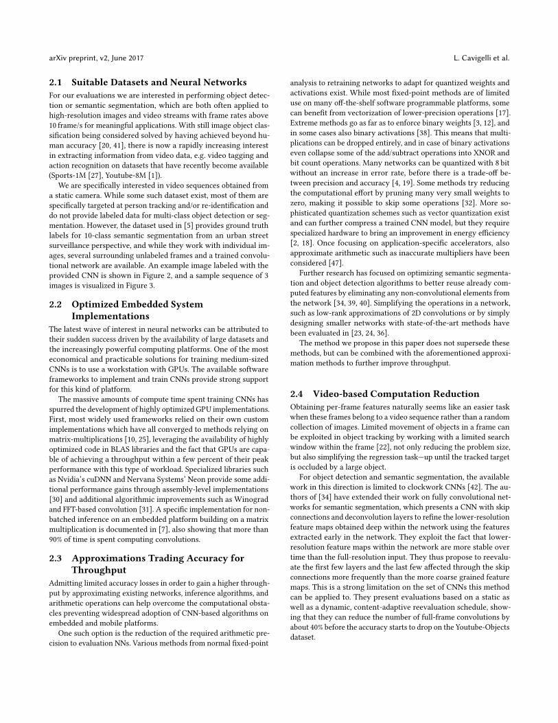
3.1 Processing StepsWe modify the standard approach and use a sequence of processingsteps (cf. Figure 4): change detection, change indexes extraction,matrix generation, matrix multiplication, and output update. In thefollowing, we will explain the individual steps.

Change Detection. In this step, changed pixels are detected. Wedefine a changed pixel as one where the absolute difference of thecurrent to the previous input of any feature map/channel exceedssome threshold τ , i.e.

m(j, i) =∨c ∈CI

|x (t )(c, j, i) − x (t−1)(c, j, i)| > τ .

The computation effort of this step is crucial, since it is executedindependently of whether any pixel changed. Each of these changesaffects a region equal to the filter size, and these output pixels aremarked for updating:

m̃(j, i) =∨

(∆j,∆i)∈Skm(j + ∆j, i + ∆i),

whereSk is the filter kernel support, e.g.Sk = {−3, . . . , 3}2 for a 7×7 filter. All of this is implemented on GPU by clearing the the changemap to all-zero and having one thread per pixel, which—if a changeis detected—sets the pixels of the filter support neighborhood inthe resulting change map.

Change Indexes Extraction. In this step, we condense the changemap m̃ to 1) a list of pixel indexes where changes occurred and2) count the number of changed pixels. This cannot easily be per-formed in parallel, so for our implementation we split the changemap into blocks of pixels, compute the result for all the blocks inparallel, and reassemble the result. The computed index list is lateron needed to access the right pixels to assemble the matrix for theconvolution.

Matrix Generation & Matrix Multiplication. Matrix multiplica-tions are used in many applications, and highly optimized imple-mentations such as the GEMM (general matrix multiplication) func-tion provided by the Nvidia cuBLAS library come within a fewpercent of the peak FLOPS of which a GPU is capable to provide.Matrix multiplication-based implementations of the convolutionlayer relying on this are widely available and are highly efficient[7, 26] and is described earlier in this section. The X matrix in (2)is not generated full-sized, but instead only those columns corre-sponding to the relevant output pixels are assembled, resulting ina reduced width equal to the number of output pixels affected bythe changes in the input image. The K matrix is made up of thefilters trained using normal convolution layers and keeps the samedimensions, so the computation effort in this step is proportional tothe number of changed pixels and the matrix multiplication is in theworst case only as time consuming as the full-frame convolution.

Output Updating. We use the previously stored results and thenewly computed output values along with the change indexes list toprovide the updated output feature maps. To maximize throughput,we also include the ReLU activation of the affected pixels in thisstep.

3.2 Memory RequirementsThe memory requirements of DNN frameworks are known to bevery high, up to the point where it becomes a limiting factor for in-creasing the mini-batch size during learning and thus reducing thethroughput when parallelizing across multiple GPUs. These require-ments are very different when looking at embedded inference-onlysystems:

(1) Inference is typically done on single frames and creatingmini-batches would introduce often unacceptable latencyand the benefit of doing so is limited to a few percent ofadditional performance [7].

(2) To maximize modularity and because it is required duringtraining, each layer typically has memory allocated to storeits output with the exception of ReLU activation layerswhich are often applied in-place.

(3) To keep a high modularity, the memory to keep the matrixX is often not shared among layers, although its values arenever reused after finishing the convolution computation.

(4) Batch normalization layers (if present) are considered in-dependent layers with their own output buffer, but theycan be absorbed into the convolution layer for inference.

To obtain a baseline memory requirement, we compute the requiredmemory of common DNN frameworks performing convolutionsusing matrix multiplication with a batch size of 1. We assume anoptimized network minimizing the number of layers, e.g. by ab-sorbing batch normalization layers into the convolution layers orusing in-place activation layers. This way 30M values need to bestored for the intermediate results, 264M values for the X matrix,and 873k values for the parameters. This can further be optimizedby sharing X among all convolution layers and by keeping onlymemory allocated to storing only the output of two layers andswitching back-and-forth between them, layer-by-layer. This re-duces the memory footprint to 9M, 93M, and 872k values, and atotal of 103M values for our baseline.

Applying our algorithm requires a little more memory, becausewe need to store additional intermediate results (cf. Figure 4) suchas the change matrix, the changed indexes list, and the Y matrix,which can all again be shared between the layers. We also needto store the previous output to use it as a basis for the updatedoutput and to use it as the previous input of the subsequent layer.For our sample network, this required another ∼ 60M values toa total of 163M values (+58%, total size ∼ 650MB)—an acceptableincrease and not a limitation, considering that modern graphicscards typically come with 8GB memory and even GPU-acceleratedembedded platforms such as the Nvidia Jetson TX1 module provide4GB of memory.

3.3 Threshold SelectionThe proposed algorithm adds one parameter to each convolutionlayer, the detection threshold. It is fixed offline after the trainingbased on sample video sequences. A threshold of zero should yieldidentical results to the non-change-based implementation, whichhas been used for functional verification. For our evaluations weused the following procedure to select the thresholds: We startby setting all thresholds to zero. Then we iteratively step through

CBinfer: Change-Based Inference for Convolutional Neural Networks on Video Data arXiv preprint, v2, June 2017

inputnin × h × w, �t

prev. input

changedetect.

changeindexesextract.

change maph × w, bool

X matrixgen.

change indexesnchg, int

matrixmultipl.

X matrixnink2 × nchg, �t

outputupdate

Y matrixnout × nchg, �t

prev. output

outputnout × h × w, �t

Figure 4: Processing flow of the change-based convolution algorithm. Custom processing kernels are shown in blue, processing steps usingavailable libraries are shown in green, variables sharable among layers are shown in yellow, and variables to be stored per-layer are coloredorange. The size and data type of the tensor storing the intermediate results is indicated below each the variable name.

Ground Truth

Frame 6

Frame 1 Frame 2 Frame 5 Frame 6

full-framechange-based change-based

evaluationNo ground truth available

...change-based

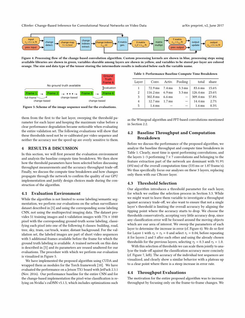
Figure 5: Scheme of the image sequence used for the evaluations.

them from the first to the last layer, sweeping the threshold pa-rameter for each layer and keeping the maximum value before aclear performance degradation became noticeable when evaluatingthe entire validation set. The following evaluations will show thatthese thresholds need not be re-calibrated per video sequence andneither the accuracy nor the speed-up are overly sensitive to them.

4 RESULTS & DISCUSSIONIn this section, we will first present the evaluation environmentand analysis the baseline compute time breakdown. We then showhow the threshold parameters have been selected before discussingthroughput measurements and the accuracy-throughput trade-off.Finally, we discuss the compute time breakdown and how changespropagate through the network to confirm the quality of our GPUimplementation and justify design choices made during the con-struction of the algorithm.

4.1 Evaluation EnvironmentWhile the algorithm is not limited to scene labeling/semantic seg-mentation, we perform our evaluations on the urban surveillancedataset described in [5] and using the corresponding scene labelingCNN, not using the multispectral imaging data. The dataset pro-vides 51 training images and 6 validation images with 776 × 1040pixel with the corresponding ground-truth scene labeling, classi-fying each pixel into one of the following 8 classes: building, road,tree, sky, tram, car/truck, water, distant background. For the val-idation set, the labeled images are part of short video sequenceswith 5 additional frames available before the frame for which theground truth labeling is available. A trained network on this datais described in [5] and its parameters are reused unaltered for ourevaluations. The procedure with which we perform our evaluationis visualized in Figure 5.

We have implemented the proposed algorithm using CUDA andwrapped them as modules for the Torch framework [10]. We haveevaluated the performance on a Jetson TX1 board with JetPack 2.3.1(Nov. 2016). Our performance baseline for the entire CNN and forthe change-based implementation the pixel-wise classification is re-lying on Nvidia’s cuDNN v5.1.5, which includes optimizations such

Table 1: Performance Baseline Compute Time Breakdown

Layer Conv. Activ. Pooling total share

1 72.9ms 7.4ms 3.3ms 83.6ms 15.6%2 116.2ms 6.9ms 3.3ms 126.4ms 23.6%3 302.8ms 6.6ms — 309.4ms 57.8%4 12.7ms 1.7ms — 14.4ms 2.7%5 1.6ms — — 1.6ms 0.3%

as the Winograd algorithm and FFT-based convolutions mentionedin Section 2.2.

4.2 Baseline Throughput and ComputationBreakdown

Before we discuss the performance of the proposed algorithm, weanalyze the baseline throughput and compute time breakdown inTable 1. Clearly, most time is spent performing convolutions, andthe layers 1–3 performing 7 × 7 convolutions and belonging to thefeature extraction part of the network are dominant with 91.9%(492ms) of the overall computation time (535ms or 1.87 frame/s).We thus specifically focus our analyses on these 3 layers, replacingonly them with our CBconv layer.

4.3 Threshold SelectionOur algorithm introduces a threshold parameter for each layer,for which we outline the selection process in Section 3.3. Whilewe might want to leave them variable to investigate a throughputagainst accuracy trade-off, we also want to ensure that not a singlelayer’s threshold is limiting the overall accuracy by aligning thetipping point where the accuracy starts to drop. We choose thethresholds conservatively, accepting very little accuracy drop, sinceany classification error will be focused around the moving objectswhich are our area of interest. We sweep the parameters of eachlayer to determine the increase in error (cf. Figure 6). We do so firstfor Layer 1 with τ2 = τ3 = 0 and select τ1 = 0.04, before repeatingit for layers 2 and 3 after each other and using the already chosenthresholds for the previous layers, selecting τ2 = 0.3 and τ3 = 1.0.

With this selection of thresholds we can scale them jointly to ana-lyze the trade-off against the classification accuracy more concisely(cf. Figure 7, left). The accuracy of the individual test sequences arevisualized, and clearly show a similar behavior with a plateau upto a clear point where there is a steep increase in error rate.

4.4 Throughput EvaluationsThe motivation for the entire proposed algorithm was to increasethroughput by focusing only on the frame-to-frame changes. We

arXiv preprint, v2, June 2017 L. Cavigelli et al.

0 5 · 10−2 0.1 0.150

0.20.40.60.8

Threshold for Layer 1 (τ1)

ErrorIncr.[%]

0 0.2 0.4 0.6 0.8 1Threshold for Layer 2 (τ2)

0 1 2 3Threshold for Layer 3 (τ3)

Figure 6: Analysis of the increase in pixel classification error rate by selecting a certain change detect threshold. This analysis is conductedlayer-by-layer, where the error increase of any layer includes the error introduced by the previous layers’ threshold choice (τ1 = 0.04, τ2 =0.3, τ3 = 1.0).

0 0.5 1 1.5 2

0

0.2

0.4

0.6

Threshold Factor

Classif.ErrorIncrease[%]

0 0.5 1 1.5 2104

105

106

Threshold Factor

#Ch

angedpixels

0 0.5 1 1.5 20

5

10

15

20

25

cuDNN

Threshold Factor

Throug

hput

[frame/s]

Figure 7: Evaluation of the impact of jointly scaling the change detection thresholds on the classification error, the number of detected changedpixels (sum over all 3 layers), and the throughput.

show the performance gain in Figure 7 (right) with the indicatedbaseline analyzing the entire frame with the same network usingcuDNN. In the extreme case of setting all thresholds to zero, theentire frame is updated, which results in a clear performance lossbecause of the change detection overhead as well as fewer opti-mization options such as less cache-friendly access patterns whengenerating the X matrix.

When increasing the threshold factor, the throughput increasesrapidly to about 16 frame/s, where it starts saturating because thechange detection step as well as other non-varying components likethe pooling and pixel classification layers are becoming dominantand the number of detected changed pixels does not further de-crease. We almost reach this plateau already for a threshold factorof 1, where we have by construction almost no accuracy loss. Theaverage frame rate over the different sequences is near 17 frame/sat this point—an improvement of 8.6× over the cuDNN baseline of1.96 frame/s.

One sequence ( ) has—while still being close to 5.1× fasterthan the baseline—a significantly lower throughput than the othersequences. While most of them show typical scenarios such asshown in Figure 3, this sequences shows a very busy situationwherethe entire road is full of vehicle and all of them are moving. Theaggregate number of changed pixels across all 3 layers is visualizedin Figure 7 (center). Most sequences trigger less than 3% of themaximum possible number of changes while the aforementionedexceptional case has a significantly higher share of around 9%.

We have repeated the same evaluations on a workstation with aNvidia GTX Titan X GPU, obtaining an almost identical throughput-threshold trade-off and compute time breakdown up to a scaling

92 94 96 980

5

10

15

20

25

cuDNN

Pixel Classification Accuracy [%]

Throug

hput

[frame/s]

Figure 8: Evaluation of the throughput-accuracy trade-off for all 6video sequences.

factor of 11.9×—as can be expected for a largely very well paral-lelizable workload and a 12× more powerful device with a similararchitecture (TX1: 512 GFLOPS and 25.6 GB/s DRAM bandwidth,GTX Titan X: 6144 GFLOPS and 336 GB/s).

4.5 Accuracy-Throughput Trade-OffWhile for some scenarios any drop in accuracy is unacceptable,many applications allow for some trade-off between accuracy andthroughput—after all choosing a specific CNN already implies se-lecting a network with an associated accuracy and computationalcost.

We analyze the trade-off directly in Figure 8. The most extremecase is updating the entire frame every time resulting in the lowest

CBinfer: Change-Based Inference for Convolutional Neural Networks on Video Data arXiv preprint, v2, June 2017

0 0.2 0.4 0.6 0.8 1 1.2 1.4 1.6 1.8

·104

L1 Conv.

L2 Conv.

L3 Conv.

Compute Time [µs]

Change Det. Change Extr. gen. X GEMM Output Upd.

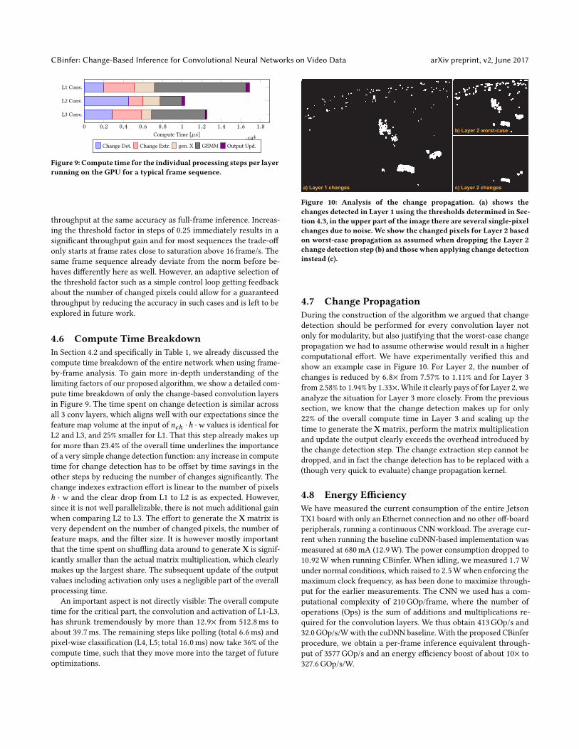
Figure 9: Compute time for the individual processing steps per layerrunning on the GPU for a typical frame sequence.

throughput at the same accuracy as full-frame inference. Increas-ing the threshold factor in steps of 0.25 immediately results in asignificant throughput gain and for most sequences the trade-offonly starts at frame rates close to saturation above 16 frame/s. Thesame frame sequence already deviate from the norm before be-haves differently here as well. However, an adaptive selection ofthe threshold factor such as a simple control loop getting feedbackabout the number of changed pixels could allow for a guaranteedthroughput by reducing the accuracy in such cases and is left to beexplored in future work.

4.6 Compute Time BreakdownIn Section 4.2 and specifically in Table 1, we already discussed thecompute time breakdown of the entire network when using frame-by-frame analysis. To gain more in-depth understanding of thelimiting factors of our proposed algorithm, we show a detailed com-pute time breakdown of only the change-based convolution layersin Figure 9. The time spent on change detection is similar acrossall 3 conv layers, which aligns well with our expectations since thefeature map volume at the input of nch ·h ·w values is identical forL2 and L3, and 25% smaller for L1. That this step already makes upfor more than 23.4% of the overall time underlines the importanceof a very simple change detection function: any increase in computetime for change detection has to be offset by time savings in theother steps by reducing the number of changes significantly. Thechange indexes extraction effort is linear to the number of pixelsh · w and the clear drop from L1 to L2 is as expected. However,since it is not well parallelizable, there is not much additional gainwhen comparing L2 to L3. The effort to generate the X matrix isvery dependent on the number of changed pixels, the number offeature maps, and the filter size. It is however mostly importantthat the time spent on shuffling data around to generate X is signif-icantly smaller than the actual matrix multiplication, which clearlymakes up the largest share. The subsequent update of the outputvalues including activation only uses a negligible part of the overallprocessing time.

An important aspect is not directly visible: The overall computetime for the critical part, the convolution and activation of L1-L3,has shrunk tremendously by more than 12.9× from 512.8ms toabout 39.7ms. The remaining steps like polling (total 6.6ms) andpixel-wise classification (L4, L5; total 16.0ms) now take 36% of thecompute time, such that they move more into the target of futureoptimizations.

a) Layer 1 changes

b) Layer 2 worst-case

c) Layer 2 changes

Figure 10: Analysis of the change propagation. (a) shows thechanges detected in Layer 1 using the thresholds determined in Sec-tion 4.3, in the upper part of the image there are several single-pixelchanges due to noise. We show the changed pixels for Layer 2 basedon worst-case propagation as assumed when dropping the Layer 2change detection step (b) and thosewhen applying change detectioninstead (c).

4.7 Change PropagationDuring the construction of the algorithm we argued that changedetection should be performed for every convolution layer notonly for modularity, but also justifying that the worst-case changepropagation we had to assume otherwise would result in a highercomputational effort. We have experimentally verified this andshow an example case in Figure 10. For Layer 2, the number ofchanges is reduced by 6.8× from 7.57% to 1.11% and for Layer 3from 2.58% to 1.94% by 1.33×. While it clearly pays of for Layer 2, weanalyze the situation for Layer 3 more closely. From the previoussection, we know that the change detection makes up for only22% of the overall compute time in Layer 3 and scaling up thetime to generate the X matrix, perform the matrix multiplicationand update the output clearly exceeds the overhead introduced bythe change detection step. The change extraction step cannot bedropped, and in fact the change detection has to be replaced with a(though very quick to evaluate) change propagation kernel.

4.8 Energy EfficiencyWe have measured the current consumption of the entire JetsonTX1 board with only an Ethernet connection and no other off-boardperipherals, running a continuous CNN workload. The average cur-rent when running the baseline cuDNN-based implementation wasmeasured at 680mA (12.9W). The power consumption dropped to10.92W when running CBinfer. When idling, we measured 1.7Wunder normal conditions, which raised to 2.5Wwhen enforcing themaximum clock frequency, as has been done to maximize through-put for the earlier measurements. The CNN we used has a com-putational complexity of 210GOp/frame, where the number ofoperations (Ops) is the sum of additions and multiplications re-quired for the convolution layers. We thus obtain 413GOp/s and32.0 GOp/s/Wwith the cuDNN baseline. With the proposed CBinferprocedure, we obtain a per-frame inference equivalent through-put of 3577GOp/s and an energy efficiency boost of about 10× to327.6 GOp/s/W.

arXiv preprint, v2, June 2017 L. Cavigelli et al.

5 CONCLUSIONWe have proposed and evaluated a novel algorithm for change-based evaluation of CNNs for video recorded with a static camerasetting, exploiting the spatio-temporal sparsity of pixel changes.The results clearly show that even when choosing the change detec-tion parameters conservatively to introduce no significant increasein misclassified pixels during semantic segmentation, an averagespeed-up of 8.6× over a cuDNN baseline has been achieved usingan optimized GPU implementation. An in-depth evaluation of thethroughput-accuracy trade-off shows the aforementioned perfor-mance jump without loss and shows how the throughput can befurther increased at the expense of accuracy. Analysis of the com-pute time split-up of the individual steps of the algorithm showthat despite some overhead the GPU is fully loaded performingmultiply-accumulate operations to update the changed pixels usingthe highly optimized cuBLAS matrix multiplication. An analysisof how changes propagate through the CNN further underline theoptimality of the structure of the proposed algorithm. The resultingboost in energy efficiency over per-frame evaluation is an averageof 10×, equivalent to 328GOp/s/W on the Tegra X1 platform.

ACKNOWLEDGMENTSThe authors would like to thank armasuisse Science & Technologyfor funding this research. This project was supported in part by theEU’s H2020 programme under grant no. 732631 (OPRECOMP).

REFERENCES[1] Sami Abu-El-Haija, Nisarg Kothari, and others. 2016. YouTube-8M: A Large-Scale

Video Classification Benchmark. (2016).[2] Alessandro Aimar, Hesham Mostafa, and others. 2017. NullHop: A Flexible

Convolutional Neural Network Accelerator Based on Sparse Representations ofFeature Maps. IEEE Transactions on Very Large Scale Integration Systems (2017).

[3] Renzo Andri, Lukas Cavigelli, and others. 2016. YodaNN: An Ultra-Low PowerConvolutional Neural Network Accelerator Based on Binary Weights. In Proc.IEEE ISVLSI. 236–241.

[4] Lukas Cavigelli and Luca Benini. 2016. Origami: A 803 GOp/s/W ConvolutionalNetwork Accelerator. IEEE TCSVT (2016).

[5] Lukas Cavigelli, Dominic Bernath, and others. 2016. Computationally efficienttarget classification in multispectral image data with Deep Neural Networks. InProc. SPIE Security + Defence, Vol. 9997.

[6] Lukas Cavigelli, David Gschwend, and others. 2015. Origami: A ConvolutionalNetwork Accelerator. In Proc. ACM GLSVLSI. ACM Press, 199–204.

[7] Lukas Cavigelli, Michele Magno, and Luca Benini. 2015. Accelerating Real-TimeEmbedded Scene Labeling with Convolutional Networks. In Proc. ACM/IEEEDAC.

[8] Yu-Hsin Chen, Tushar Krishna, and others. 2016. Eyeriss: An energy-efficientreconfigurable accelerator for deep convolutional neural networks. In Proc. IEEEISSCC. 262–263.

[9] Sharan Chetlur, Cliff Woolley, and others. 2014. cuDNN: Efficient Primitives forDeep Learning.

[10] Ronan Collobert. 2011. Torch7: AMatlab-like Environment for Machine Learning.Advances in Neural Information Processing Systems Workshops (2011).

[11] Marius Cordts, Mohamed Omran, and others. 2016. The Cityscapes Dataset forSemantic Urban Scene Understanding. In Proc. IEEE CVPR. 3213–3223.

[12] Matthieu Courbariaux, Yoshua Bengio, and Jean-Pierre David. 2015. BinaryCon-nect: Training Deep Neural Networks with binary weights during propagations.In Adv. NIPS. 3105–3113.

[13] Jia Deng, Wei Dong, and others. 2009. ImageNet: A large-scale hierarchical imagedatabase. In Proc. IEEE CVPR.

[14] Clement Farabet, Berin Martini, and others. 2011. NeuFlow: A Runtime Recon-figurable Dataflow Processor for Vision. In Proc. IEEE CVPRW. 109–116.

[15] Nicolas Farrugia, Franck Mamalet, and others. 2009. Fast and Robust FaceDetection on a Parallel Optimized Architecture Implemented on FPGA. IEEETCSVT 19, 4 (2009), 597–602.

[16] Philipp Fischer, Alexey Dosovitskiy, and others. 2015. FlowNet: Learning OpticalFlow with Convolutional Networks. In arXiv:15047.06852.

[17] Philipp Gysel, Mohammad Motamedi, and Soheil Ghiasi. 2016. Hardware-oriented Approximation of Convolutional Neural Networks. In ICLR Workshops.

[18] Song Han, Xingyu Liu, and others. 2016. EIE: Efficient Inference Engine onCompressed Deep Neural Network. arXiv:1602.01528 (2016).

[19] Soheil Hashemi, Nicholas Anthony, and others. 2016. Understanding the Impactof Precision Quantization on the Accuracy and Energy of Neural Networks.arXiv:1612.03940 (2016).

[20] Kaiming He, Xiangyu Zhang, and others. 2015. Deep Residual Learning forImage Recognition. Proc. IEEE CVPR (2015), 770–778.

[21] Kaiming He, Xiangyu Zhang, and others. 2015. Delving Deep into Rectifiers:Surpassing Human-Level Performance on ImageNet Classification.

[22] David Held, Sebastian Thrun, and Silvio Savarese. 2016. Learning to track at 100FPS with deep regression networks. LNCS 9905 (2016), 749–765.

[23] Forrest N. Iandola, Matthew W. Moskewicz, and others. 2016. SqueezeNet:AlexNet-Level Accuracy with 50x Fewer Parameters and 1MB Model Size.arXiv:1602.07360 (2016).

[24] Max Jaderberg, Andrea Vedaldi, and A Zisserman. 2014. Speeding up Convolu-tional Neural Networks with Low Rank Expansions. In arXiv:1405.3866.

[25] Yangqing Jia. 2013. Caffe: An Open Source Convolutional Architecture for FastFeature Embedding. (2013). http://caffe.berkeleyvision.org

[26] Jonghoon Jin, Vinayak Gokhale, and others. 2014. An efficient implementationof deep convolutional neural networks on a mobile coprocessor. In Proc. IEEEMWSCAS’14. 133–136.

[27] Andrej Karpathy, George Toderici, and others. 2014. Large-scale video classifica-tion with convolutional neural networks. Proc. IEEE CVPR (2014), 1725–1732.

[28] Alex Krizhevsky, Ilya Sutskever, and Geoffrey E Hinton. 2012. Imagenet Classifi-cation With Deep Convolutional Neural Networks. In Adv. NIPS.

[29] Herman Kruegle. 1995. CCTV Surveillance: Video Practices and Technology.Butterworth-Heinemann, Woburn, MA, USA.

[30] Andrew Lavin. 2015. maxDNN: An Efficient Convolution Kernel for Deep Learn-ing with Maxwell GPUs. In arXiv:1501.06633v3.

[31] Andrew Lavin and Scott Gray. 2016. Fast Algorithms for Convolutional NeuralNetworks. In Proc. IEEE CVPR. 4013–4021.

[32] Hao Li, Asim Kadav, and others. 2016. Pruning Filters for Efficient ConvNets.arXiv:1608.08710 (2016).

[33] Tsung-Yi Lin, Michael Maire, and others. 2014. Microsoft COCO: CommonObjects in Context. In Proc. ECCV.

[34] Jonathan Long, Evan Shelhamer, and Trevor Darrell. 2015. Fully ConvolutionalNetworks for Semantic Segmentation. In Proc. IEEE CVPR.

[35] Woon-sung Park and Munchurl Kim. 2016. CNN-based in-loop filtering forcoding efficiency improvement. In Proc. IEEE Image, Video, and MultidimensionalSignal Processing Workshop.

[36] Adam Paszke, Abhishek Chaurasia, and others. 2016. ENet: A Deep NeuralNetworkArchitecture for Real-Time Semantic Segmentation. In arXiv:1609.02147.

[37] Fatih Porikli, Francois Bremond, and others. 2013. Video surveillance: past,present, and now the future [DSP Forum]. IEEE Signal Processing Magazine 30(2013), 190–198.

[38] Mohammad Rastegari, Vicente Ordonez, and others. 2016. XNOR-Net: ImageNetClassification Using Binary Convolutional Neural Networks. In arXiv:1603.05279.

[39] Joseph Redmon, Santosh Divvala, and others. 2016. You Only Look Once: Unified,Real-Time Object Detection.

[40] Shaoqing Ren, Kaiming He, and others. 2015. Faster R-CNN: Towards Real-TimeObject Detection with Region Proposal Networks. arXiv:1506.01497 (2015).

[41] Olga Russakovsky, Jia Deng, and others. 2015. ImageNet Large Scale VisualRecognition Challenge. IJCV 115, 3 (2015), 211–252.

[42] Evan Shelhamer, Kate Rakelly, and others. 2016. Clockwork Convnets for VideoSemantic Segmentation. arXiv:1608.03609 (2016).

[43] Christian Szegedy, Wei Liu, and others. 2015. Going Deeper with Convolutions.In Proc. IEEE CVPR.

[44] Nicolas Vasilache, Jeff Johnson, and others. 2014. Fast Convolutional Nets Withfbfft: A GPU Performance Evaluation. arXiv:1412.7580 (2014).

[45] Chen Zhang, Zhenman Fang, and others. 2016. Caffeine: Towards UniformedRepresentation and Acceleration for Deep Convolutional Neural Networks. InProc. ACM ICCAD. New York, NY, USA.

[46] Kaihua Zhang, Qingshan Liu, and others. 2016. Robust Visual Tracking viaConvolutional Networks without Training. IEEE TIP (2016).

[47] Qian Zhang, Ting Wang, and others. 2015. ApproxANN: An ApproximateComputing Framework for Artificial Neural Network. In Proc. IEEE DATE.