chap-3 cfd
DESCRIPTION
fffTRANSCRIPT
Chap. 3 Methods of
Numerical Analysis

3.1 Numerical Procedure
PDEElliptic typeParabolic typeHyperbolic type
FDMFVMFEM
Grid or Mesh Generation
What’s your governing eq
(PDE) ?
Identify PDE type:
Apply IC and/or BC
Discretization :
Apply numerical scheme that you want
Solution Post-processing

Type of Numerical Approach
FDM (Finite Difference Method, 유한차분법)
FVM (Finite Volume Method, 유한체적법)
FEM (Finite Element Method, 유한요소법)
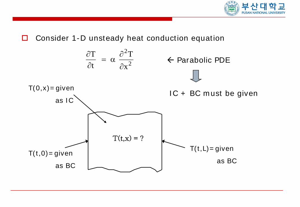
Consider 1-D unsteady heat conduction equation
Parabolic PDE
IC + BC must be given
∂∂
α∂
∂
Tt
Tx
=2
2
T(t,x) = ?
T(t,0)=given
as BC
T(t,L)=given
as BC
T(0,x)=given
as IC

T(t,x) = ?
T(t,0)=given
as BC
T(t,L)=given
as BC
T(0,x)=given
as IC
T(n,1) = Given 4 T(n,11) = Given
as B.C. 3 as B.C.
t
x
6
5 T(n,i) = ?
n=0
n=1 T(0,i) = Givenas I.C.
2
i=1 2 3 4 5 6 7 8 9 10 11
x=0 x=L

3.1 FDM (Finite Difference Method)
FDM may use polynomial, sin/cos, Legendre polynomial,
Fouries, or Taylor series expansion.
But, Taylor series expansion is mostly used.
DNS usually uses Fourier series expansion.
Taylor series expansion in time :
( ) ( )( ) ( ) ( )
( )∞+⋅⋅⋅⋅⋅+
∆+⋅⋅⋅⋅⋅
∆+
∆+∆+=∆+
!
+
!3
2
, ,
,
,3
33
,2
22
,
xtn
nn
xtxtxt
tT
nt
tTt
tTt
tTtxtTxttT
∂∂
∂∂
∂∂
∂∂
Brook Taylor (1685-1731)- born in Edmonton, Middlesex, England
http://numericalmethods.eng.usf.edu/topics/comprehensive_index.htmlhttp://numericalmethods.eng.usf.edu/

Rewriting as tT∂∂
( )
( ) ( )( ) ( )
∂∂
∂
∂
∂
∂
Tt
T t t x T t xt
t Tt
t Ttt x t x t x, , ,
, ,=
+ −− − − ⋅ ⋅ ⋅ ⋅ ⋅ − ∞
∆∆
∆ ∆2 6
2
2
2 3
3
( )
( ) ( )∂∂Tt
T t t x t xt
tt x,
, ,( )
T O≈
+ −+
∆∆
∆
Truncation (Discretization) Error
1st order accurate in time

Taylor series expansion in space(x-axis):
( ) ( )( ) ( ) ( )
( )
T t x x t x x Tx
x Tx
x Tx
x Tx
t x t x t x
t x
, ,!
!
, , ,
,
+ = + + +
+ + ⋅ ⋅ ⋅ ⋅ ⋅ + ∞
∆ ∆∆ ∆
∆
T
∂∂
∂
∂
∂
∂
∂
∂
2 2
2
3 3
3
4 4
4
2 3
4
( ) ( )( ) ( ) ( )
( )
T t x x t x x Tx
x Tx
x Tx
x Tx
t x t x t x
t x
, ,!
!
, , ,
,
− = − + −
+ − ⋅ ⋅ ⋅ ⋅ ⋅ + ∞
∆ ∆∆ ∆
∆
T
∂∂
∂
∂
∂
∂
∂
∂
2 2
2
3 3
3
4 4
4
2 3
4
(a)
(b)

Adding (a) and (b) and, then, write in terms of ∂ ∂2 2T(t x x, )
( )
( ) ( ) ( )
( ) ( )
∂
∂
∂
∂
∂
∂
2
2 2
2 4
4
4 6
6
2
24
26!
Tx
T t x x t x t x xx
x Tx
x Tx
t x
t x t x
,
, ,
, , ,
!
=+ − + −
− − − ⋅ ⋅ ⋅ ⋅ ⋅ − ∞
T T
∆ ∆
∆
∆ ∆
( )
( ) ( ) ( ) ( )∂
∂
2
2 222T
xT t x x t x t x x
xx
t x,
, , ,≈
+ − + −+
T T O
∆ ∆
∆∆
Approximately,
2nd order accurate in space

In summary,
Governing eq. : ∂∂
α∂
∂
Tt
Tx
=2
2
( )
( ) ( )∂∂Tt
T t t x t xt
tt x,
, ,( )
T O≈
+ −+
∆∆
∆
( )
( ) ( ) ( ) ( )∂
∂
2
2 222T
xT t x x t x t x x
xx
t x,
, , ,≈
+ − + −+
T T O
∆ ∆
∆∆
From Taylor series expansion,

To simplify the equation, the following notations are
introduced:
( ) ( ) ( ) ( ) ( ) ( )T t t x T t xt
T t x x T t x T t x xx
O t x+ −
=+ − + −
+∆
∆∆ ∆
∆∆ ∆
, , , , ,,α
22
2
( )( )( )( )
T t x T
T t t x T
T t x x T
T t x x T
in
in
in
in
,
,
,
,
=
+ =
+ =
− =
+
+
−
∆
∆
∆
1
1
1

Then,
( )Tt
Tx
t xin
in
in
in
in+
+ −−=
− ++
11 1
222 T
T T
O∆ ∆
∆ ∆α ,
“Finite-Difference Equation”
1st order accurate in time
and 2nd order accurate in space

Rewrite in terms of
2 2
111
xTTT
tTT n
in
in
in
in
i
∆+−
≈∆− −+
+α
1+niT
( )Tin
in
in
in
in+
+ −= + − +11 12 T d T T T
whered t
x=α ∆∆ 2 : Diffusion number

Example 1.
i=1 2 3 4 5
BC : T(t,0)=10oC BC : T(t,L)=50oC
IC : )5~1 ( 1000 == iforCT oi
Tin+ =1 ?
L

Assume =0.3
While n=0,
(1) at i=2, =73oC
(2) at i=3, =100oC
d tx
=α ∆∆ 2
( )Tin
in
in
in
in+
+ −= + − +11 12 T d T T T
( ) 2 0.3 111 n
in
in
in
in
i TTTTT −++ +−+=
( ) 2 0.3 01
02
03
02
12 TTTTT +−+=
100oC 100oC 100oC 10oC
i=1 2 3 4 5
BC: BC:T(t,0)=10oC T(t,L)=50oC
IC : )5~1 ( 1000 == iforCT oi
Tin+ =1 ?
( ) 2 0.3 02
03
04
03
13 TTTTT +−+=
100oC 100 100 100

(1) at i=4,
( ) 2 0.3 111 n
in
in
in
in
i TTTTT −++ +−+=
( ) 2 0.3 03
04
05
04
14 TTTTT +−+=
100oC 10010050oC
i=1 2 3 4 5
BC: BC:T(t,0)=10oC T(t,L)=50oC
IC : )5~1 ( 1000 == iforCT oi
Tin+ =1 ?
= 85oC

i=1 2 3 4 5
BC : T(t,0)=10oC BC : T(t,L)=50oC
IC : )5~1 ( 1000 == iforCT oi
Tin+ =1 ?
L
i=1 2 3 4 5
10
100
50
73
85
After ∆t
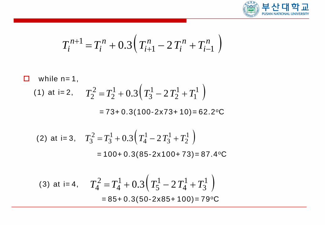
while n=1,
(1) at i=2,
(2) at i=3,
(3) at i=4,
( ) 2 0.3 111 n
in
in
in
in
i TTTTT −++ +−+=
( ) 2 0.3 11
12
13
12
22 TTTTT +−+=
=73+0.3(100-2x73+10)=62.2oC
( ) 2 0.3 12
13
14
13
23 TTTTT +−+=
=100+0.3(85-2x100+73)=87.4oC
( ) 2 0.3 13
14
15
14
24 TTTTT +−+=
=85+0.3(50-2x85+100)=79oC

i=1 2 3 4 5
10
100
50
73
85
After 2∆t
62.2
87.479

while n=2,
(1) at i=2,
(2) at i=3,
(3) at i=4,
( ) 2 0.3 111 n
in
in
in
in
i TTTTT −++ +−+=
( ) 2 0.3 21
22
23
22
32 TTTTT +−+=
=62.2+0.3(87.4-2x62.2+10)=oC
( ) 2 0.3 22
23
24
23
33 TTTTT +−+=
=87.4+0.3(79-2x87.4+62.2)=oC
( ) 2 0.3 23
24
25
24
34 TTTTT +−+=
=79+0.3(50-2x79+87.4)=oC

i=1 2 3 4 5
10
100
50
After 2∆t
Steady state solution

Repeat until the steady state approaches.
The present algorithm is called “explicit time marching
scheme”.
0 .,.
0
1
4~2≈−
=
+
=
ni
ni
iTTei
tT
Max∂∂

3.2 FVM (Finite-Volume Method)
FVM solves the following integral equation, rather than
differential equation.
Substitute our PDE into the above integral equation,
[ ]Physicalspace
PDE dV ≡∫∫∫ 0
At eachnode i
Tt
Tx
dx ∂∂
α∂
∂−
≡∫2
2 0
Control volume
i-1 i i+1

Applying each control volume (i-1/2 ~ i+1/2),
Here, we define the average value, Ti, as:
Then,
dx ∂∂
α∂
∂
Tt
Txx x
x x
i
i−
=−
+
∫2
22
20
∆
∆
/
/
Txi
x x
x x
i
i T dx=
−
+
∫12
2
∆ ∆
∆
/
/
Term#1 = ∂∂Tt
dxx x
x x
i
i
−
+
∫ ∆
∆
/
/
2
2 [ ] T 2/2/ dx
dtd xx
xxi
i∫
∆+∆−
=
( integral domain i±1/2 is indep to time)

Thus,
Similarly,
[ ] ( ) xdtdTxTdx
dtdTerm i
idtdxx
xxi
i∆=∆== ∫
∆+∆−
T 1# 2/2/
Txi
x x
x x
i
i T dx=
−
+
∫12
2
∆ ∆
∆
/
/
2# 2/2/ 2
2dx
xTTerm xx
xxi
i∫
∆+∆−
=
∂∂α
−=
∆−∆+
2/2/ xxxx iixT
xT
∂∂
∂∂α

Therefore,
dx ∂∂
α∂
∂
Tt
Txx x
x x
i
i−
=−
+
∫2
22
20
∆
∆
/
/
∆∆ ∆
x dTdt
Tx
Tx
i
x x x xi i
= −
+ −
α∂∂
∂∂/ /2 2
( )dTdt
T Tt
O ti in
in
=−
++1
∆∆ ( )∂
∂Tx
T Tx
O xx x
in
in
i−
−=−
+∆ ∆
∆/2
1 2
( )∂∂Tx
T Tx
O xx x
in
in
i+
+=−
+∆ ∆
∆/2
1 2
Taylor series expn
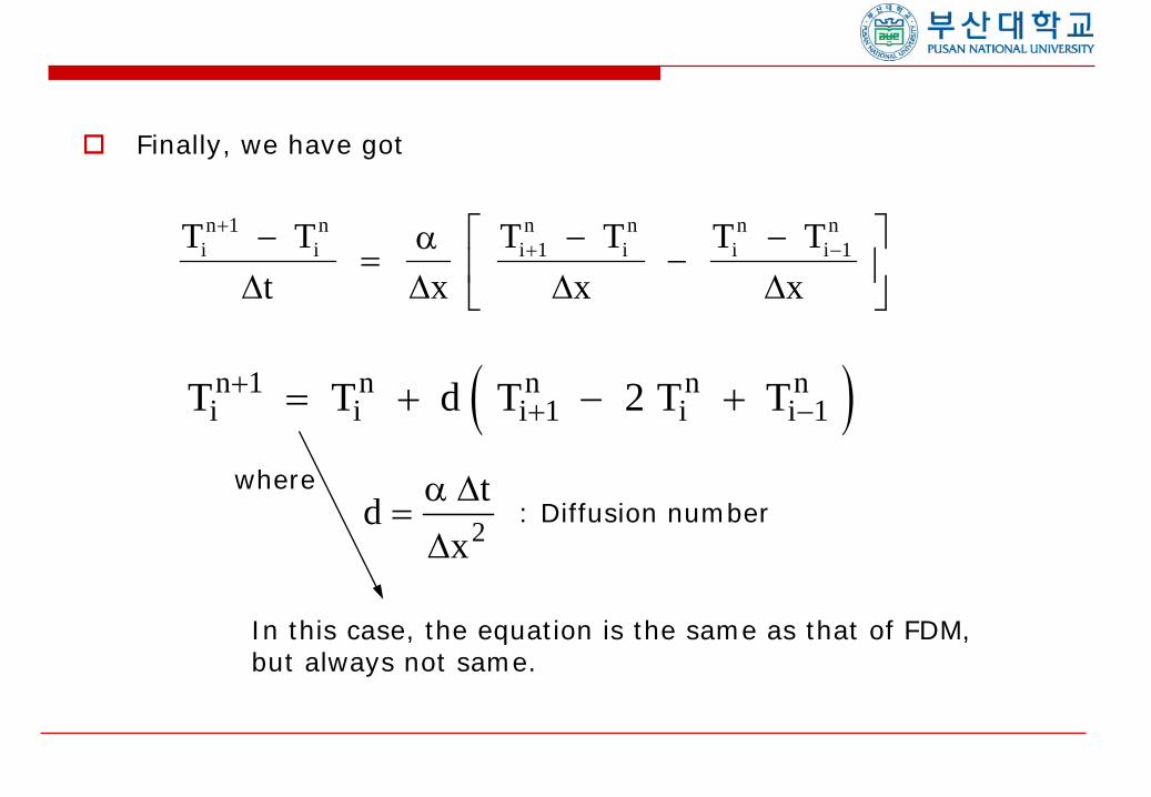
Finally, we have got
( )Tin
in
in
in
in+
+ −= + − +11 12 T d T T T
Tt x
Tx
Tx
in
in
in
in
in
in+
+ −−=
−−
−
11 1 T T T
∆ ∆ ∆ ∆α
whered t
x=α ∆∆ 2
: Diffusion number
In this case, the equation is the same as that of FDM, but always not same.

Solution procedure is the same as that of FDM.
(a) While n=0,
(1) at i=2,
=73oC
(2) at i=3, =100oC
( )Tin
in
in
in
in+
+ −= + − +11 12 T d T T T
( ) 2 0.3 111 n
in
in
in
in
i TTTTT −++ +−+=
( ) 2 0.3 01
02
03
02
12 TTTTT +−+=
100oC 100oC 100oC 10oC
i=1 2 3 4 5
BC: BC:T(t,0)=10oC T(t,L)=50oC
IC : )5~1 ( 1000 == iforCT oi
Tin+ =1 ?
( ) 2 0.3 02
03
04
03
13 TTTTT +−+=
100oC 100 100 100
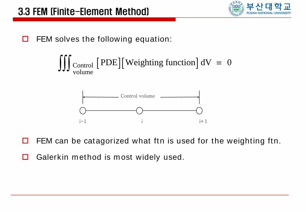
3.3 FEM (Finite-Element Method)
FEM solves the following equation:
FEM can be catagorized what ftn is used for the weighting ftn.
Galerkin method is most widely used.
[ ] [ ]Controlvolume
PDE Weighting function dV ∫∫∫ ≡ 0
Control volume
i-1 i i+1

Galerkin Method:
- uses the same order of polynomial ftn that is used to
approximate the unknown(s).
( ) 0 1
12
2≡
−∫
+
−
dxxwxT
tTi
i
x
x ∂∂α
∂∂
( )dxxwtTTerm i
i
x
x 1# 1
1∫
+
−
=∂∂ ( ) ( )dxxw
tTdxxw
tT i
i
i
i
x
x
x
x 1
1∫∫
+
−
+=∂∂
∂∂
( ) ( )
+= ∫∫
+
−
dxxwdxxwt
i
i
i
i
x
x
x
x T T 1
1∂∂
t∂∂
= { ϑ1 + ϑ2 }

where ( ) ; T1
1 dxxwi
i
x
x∫ −
=ϑ ( )ϑ21
= T dxx
x
i
iw x
+
∫T(x)
i-1 i i+1 x
w(x)
1
0
i-1 i i+1 x
1st order polynomial ftn for unknown, T
1st order polynomial ftn for weighting, w
Ti-1
Ti
Ti+1
Galerkin: Same order of poly
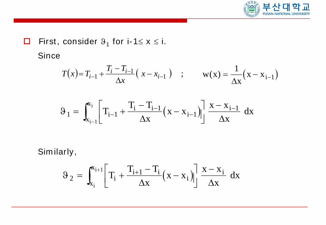
First, consider ϑ1 for i-1≤ x ≤ i.
Since
Similarly,
( ) ( ) ; 11
1 −−
− −∆−
+= iii
i xxxTTTxT ( )w x
xx xi( ) = − −
11∆
( )ϑ1 11
11
1
= +−
−
−−
−−
−
−∫ T T T
xx x x x
xii i
ix
x i
i
i
∆ ∆ dx
( )ϑ211
= +−
−
−++
∫ T T Tx
x x x xxi
i ii
x
x i
i
i
∆ ∆ dx

Thus,
tTerm
∂∂
=1# { ϑ1 + ϑ2 }
dtdT
dtdT
dtdT iii 11
61
32
61 +− ++=
∆−
+
∆−
+
∆−
= +++
+−
+−
tTT
tTT
tTT n
in
in
in
in
in
i 11
11
11
1 61
32
61

whereas,
Here, partial integration was used.
dxxwxTTerm i
i
x
x )( 2# 1
12
2
∫+
−
=∂∂α
dxxT
xxw
xTxw
i
i
x
x )( )( 1+i
1-i
1
1
x
x ∂∂
∂∂α
∂∂α ∫−
=
+
−
[ ] P dx dQdx
PQ dPdx
Q dxa
b
ab
a
b= −∫ ∫

dxxT
xxw
xTxwTerm
i
i
x
x )( )( 2# 1+i
1-i
1
1
x
x ∂∂
∂∂α
∂∂α ∫−
=
+
−
dxxT
xxw )( 1+i
1-i
x
x ∂∂
∂∂α ∫−=
(because w(x)=0 at xi±1)
w(x)
1
0
i-1 i i+1 x
dxxT
xwdx
xT
xwTerm ii
i
x
x
x
x 2# 1
11 ∂∂
∂∂α
∂∂
∂∂α ∫∫
+
−
−−=

dxxT
xwdx
xT
xwTerm ii
i
x
x
x
x 2# 1
11 ∂∂
∂∂α
∂∂
∂∂α ∫∫
+
−
−−=
( )
∆∆−
∆−
+∆∆
∆−
−= +−
xx
xTT
xx
xTT iiii 1 11α
[ ] 2 11 −+ +−∆
= iii TTTxα
Therefore, the final equation by FEM is
16
23
16
11
11
11
1 T
T
TT
tT
tT
tin
in
in
in
in
in
−+
−+
++
+−
+
−
+
−
∆ ∆ ∆
[ ] 2 11 −+ +−∆
= iii TTTxα