chapter 4: generalized predictive controlfumblog.um.ac.ir/gallery/839/mpc_lecture_92_4_1.pdf ·...
TRANSCRIPT
CHAPTER 4:
Generalized Predictive Control
1
S.K. Hosseini Sani
Assistant Professor
Electrical Engineering
Ferdowsi University
Mashhad, Iran1392
Generalized Predictive Control
2
4.1 Introduction
1987سالدرclarkeتوسطGPCکنترلطرح•
تحقیقوپژوهشدروصنعتدرمحبوبروش•
فرآیندتبدیلتابعمدلبرمتکی•
ناپایداروفازمینیممغیرسیستمهایبهاعمالقابلیت•
3
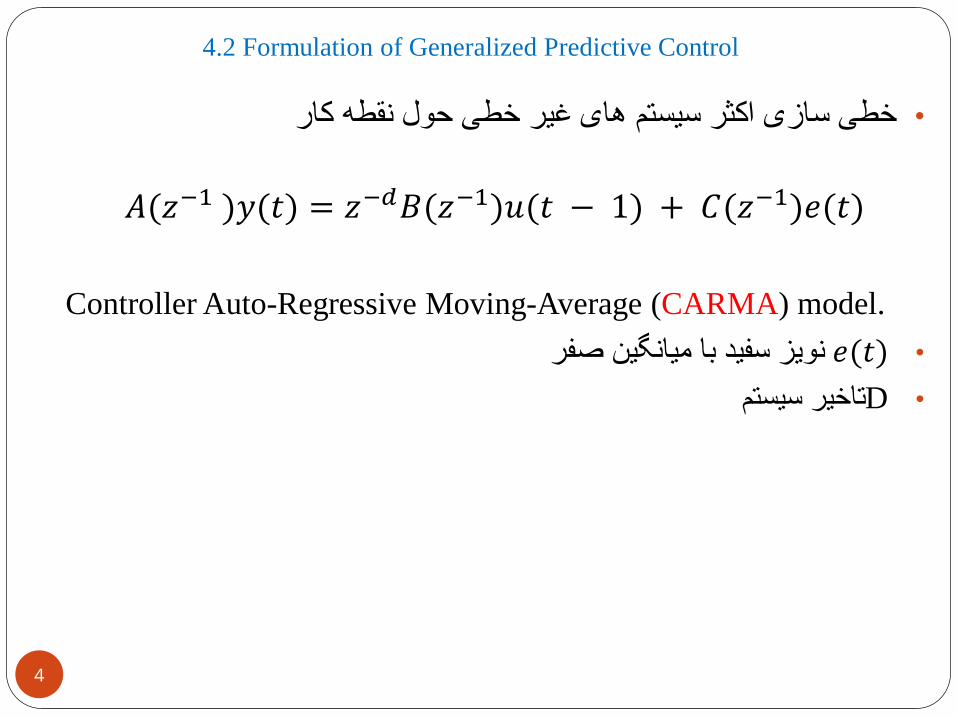
4.2 Formulation of Generalized Predictive Control
کارنقطهحولخطیغیرهایسیستماکثرسازیخطی•
𝐴(𝑧−1 )𝑦(𝑡) = 𝑧−𝑑𝐵(𝑧−1)𝑢(𝑡 − 1) + 𝐶(𝑧−1)𝑒(𝑡)
Controller Auto-Regressive Moving-Average (CARMA) model.
•𝑒(𝑡)صفرمیانگینباسفیدنویز
•Dسیستمتاخیر
4
4.2 Formulation of Generalized Predictive Control
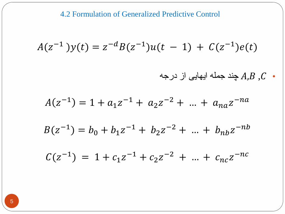
𝐴(𝑧−1 )𝑦(𝑡) = 𝑧−𝑑𝐵(𝑧−1)𝑢(𝑡 − 1) + 𝐶(𝑧−1)𝑒(𝑡)
•𝐴,𝐵 ,𝐶درجهازایهاییجملهچند
𝐴 𝑧−1 = 1 + 𝑎1𝑧−1 + 𝑎2𝑧−2 + … + 𝑎𝑛𝑎𝑧−𝑛𝑎
𝐵(𝑧−1) = 𝑏0 + 𝑏1𝑧−1 + 𝑏2𝑧−2 + … + 𝑏𝑛𝑏𝑧−𝑛𝑏
𝐶(𝑧−1) = 1 + 𝑐1𝑧−1 + 𝑐2𝑧−2 + … + 𝑐𝑛𝑐𝑧
−𝑛𝑐
5
4.2 Formulation of Generalized Predictive Control
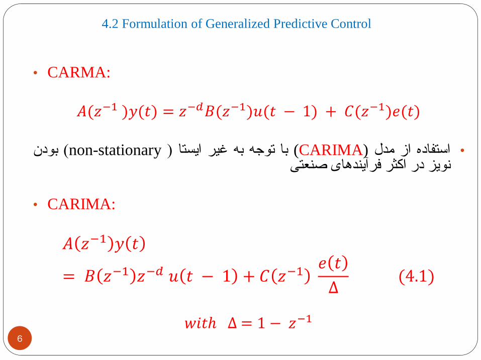
• CARMA:
𝐴(𝑧−1 )𝑦(𝑡) = 𝑧−𝑑𝐵(𝑧−1)𝑢(𝑡 − 1) + 𝐶(𝑧−1)𝑒(𝑡)
بودن(non-stationary)ایستاغیربهتوجهبا(CARIMA)مدلازاستفاده•صنعتیفرآیندهایاکثردرنویز
• CARIMA:
𝐴 𝑧−1 𝑦 𝑡
= 𝐵 𝑧−1 𝑧−𝑑 𝑢 𝑡 − 1 + 𝐶 𝑧−1𝑒 𝑡
∆(4.1)
𝑤𝑖𝑡ℎ ∆ = 1 − 𝑧−1
6
4.2 Formulation of Generalized Predictive Control
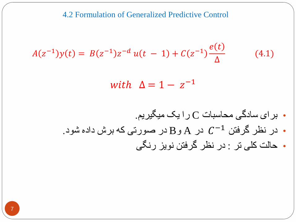
𝐴 𝑧−1 𝑦 𝑡 = 𝐵 𝑧−1 𝑧−𝑑 𝑢 𝑡 − 1 + 𝐶 𝑧−1𝑒 𝑡
∆(4.1)
𝑤𝑖𝑡ℎ ∆ = 1 − 𝑧−1
.میگیریمیکراCمحاسباتسادگیبرای•
.شوددادهبرشکهصورتیدرBوAدر𝐶−1گرفتننظردر•
رنگینویزگرفتننظردر:ترکلیحالت•
7
4.2 Formulation of Generalized Predictive Control
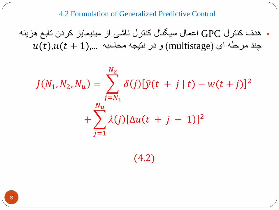
هزینهتابعکردنمینیمایزازناشیکنترلسیگنالاعمالGPCکنترلهدف•
𝑢(𝑡),𝑢(𝑡محاسبهنتیجهدرو(multistage)ایمرحلهچند + 1),...
𝐽 𝑁1, 𝑁2, 𝑁𝑢 =
𝑗=𝑁1
𝑁2
𝛿 𝑗 𝑦(𝑡 + 𝑗 | 𝑡) − 𝑤(𝑡 + 𝑗) 2
+
𝑗=1
𝑁𝑢
𝜆 𝑗 ∆𝑢 𝑡 + 𝑗 − 1 2
(4.2)
8
4.2 Formulation of Generalized Predictive Control
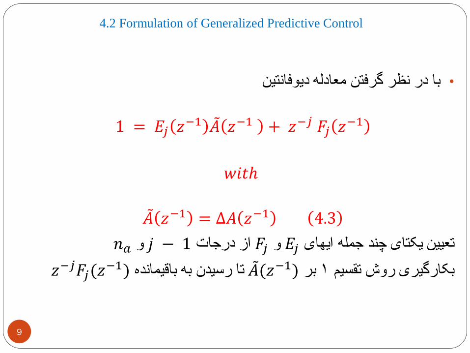
دیوفانتینمعادلهگرفتننظردربا•
1 = 𝐸𝑗 𝑧−1 𝐴 𝑧−1 + 𝑧−𝑗 𝐹𝑗 𝑧−1
𝑤𝑖𝑡ℎ
𝐴 𝑧−1 = ∆𝐴 𝑧−1 4.3
𝑗درجاتاز𝐹𝑗و𝐸𝑗ایهایجملهچندیکتایتعیین − 𝑛𝑎و1
𝑧−𝑗𝐹𝑗(𝑧باقیماندهبهرسیدنتا𝐴(𝑧−1) بر1تقسیمروشبکارگیری−1)
9
4.2 Formulation of Generalized Predictive Control
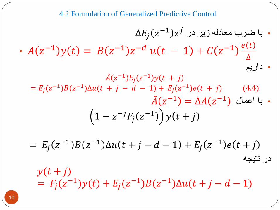
𝐸𝑗∆درزیرمعادلهضرببا• 𝑧−1 𝑧𝑗
• 𝐴 𝑧−1 𝑦 𝑡 = 𝐵 𝑧−1 𝑧−𝑑 𝑢 𝑡 − 1 + 𝐶 𝑧−1 𝑒 𝑡
∆
داریم• 𝐴 𝑧−1 𝐸𝑗 𝑧−1 𝑦 𝑡 + 𝑗
= 𝐸𝑗(𝑧−1)𝐵(𝑧−1)∆𝑢(𝑡 + 𝑗 − 𝑑 − 1) + 𝐸𝑗(𝑧
−1)𝑒(𝑡 + 𝑗) (4.4)
𝐴 اعمالبا• 𝑧−1 = ∆𝐴 𝑧−1
1 − 𝑧−𝑗𝐹𝑗 𝑧−1 𝑦 𝑡 + 𝑗
= 𝐸𝑗 𝑧−1 𝐵 𝑧−1 ∆𝑢 𝑡 + 𝑗 − 𝑑 − 1 + 𝐸𝑗 𝑧−1 𝑒 𝑡 + 𝑗
نتیجهدر
𝑦(𝑡 + 𝑗)= 𝐹𝑗(𝑧
−1)𝑦(𝑡) + 𝐸𝑗(𝑧−1)𝐵(𝑧−1)∆𝑢(𝑡 + 𝑗 − 𝑑 − 1)
10
4.2 Formulation of Generalized Predictive Control
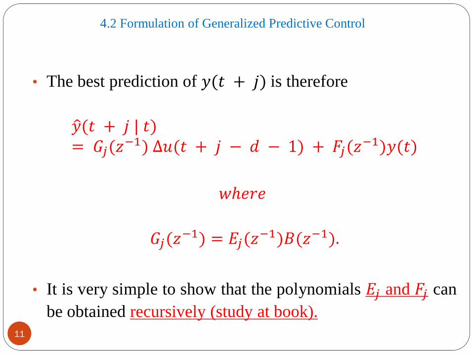
• The best prediction of 𝑦(𝑡 + 𝑗) is therefore
𝑦(𝑡 + 𝑗 | 𝑡)= 𝐺𝑗(𝑧
−1) ∆𝑢(𝑡 + 𝑗 − 𝑑 − 1) + 𝐹𝑗(𝑧−1)𝑦(𝑡)
𝑤ℎ𝑒𝑟𝑒
𝐺𝑗(𝑧−1) = 𝐸𝑗(𝑧
−1)𝐵(𝑧−1).
• It is very simple to show that the polynomials 𝐸𝑗 and 𝐹𝑗 can
be obtained recursively (study at book).
11
4.2 Formulation of Generalized Predictive Control
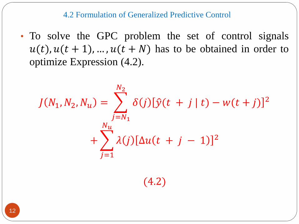
• To solve the GPC problem the set of control signals
𝑢(𝑡), 𝑢(𝑡 + 1), … , 𝑢(𝑡 + 𝑁) has to be obtained in order to
optimize Expression (4.2).
𝐽 𝑁1, 𝑁2, 𝑁𝑢 =
𝑗=𝑁1
𝑁2
𝛿 𝑗 𝑦(𝑡 + 𝑗 | 𝑡) − 𝑤(𝑡 + 𝑗) 2
+
𝑗=1
𝑁𝑢
𝜆 𝑗 ∆𝑢 𝑡 + 𝑗 − 1 2
(4.2)
12
4.2 Formulation of Generalized Predictive Control
13
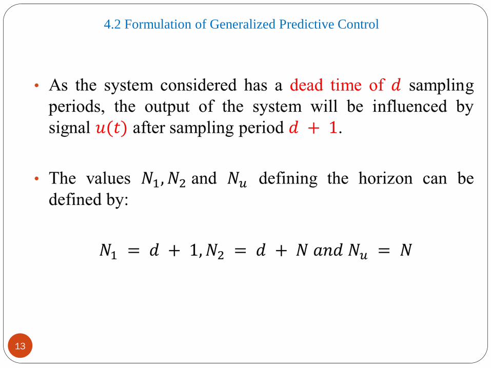
4.2 Formulation of Generalized Predictive Control
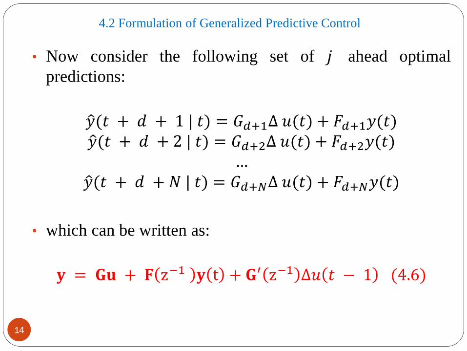
• Now consider the following set of 𝑗 ahead optimal
predictions:
𝑦(𝑡 + 𝑑 + 1 | 𝑡) = 𝐺𝑑+1∆ 𝑢(𝑡) + 𝐹𝑑+1𝑦(𝑡) 𝑦(𝑡 + 𝑑 + 2 | 𝑡) = 𝐺𝑑+2∆ 𝑢(𝑡) + 𝐹𝑑+2𝑦(𝑡)
… 𝑦(𝑡 + 𝑑 + 𝑁 | 𝑡) = 𝐺𝑑+𝑁∆ 𝑢(𝑡) + 𝐹𝑑+𝑁𝑦(𝑡)
• which can be written as:
𝐲 = 𝐆𝐮 + 𝐅 z−1 𝐲 t + 𝐆′ z−1 ∆𝑢 𝑡 − 1 (4.6)
14
4.2 Formulation of Generalized Predictive Control
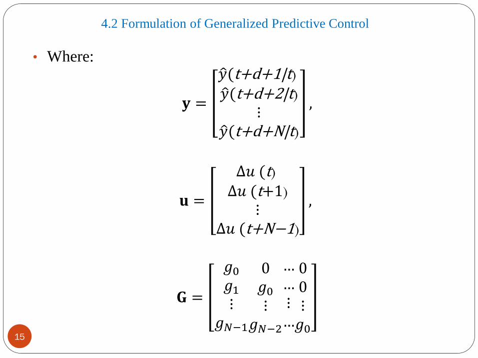
• Where:
𝐲 =
𝑦(t+d+1|t) 𝑦(t+d+2|t)
⋮ 𝑦(t+d+N|t)
,
𝐮 =
∆𝑢 (t)∆𝑢 (t+1)
⋮∆𝑢 (t+N−1)
,
𝐆 =
𝑔0
𝑔1
⋮𝑔𝑁−1
0𝑔0
⋮𝑔𝑁−2
……⋮…
00⋮
𝑔015
4.2 Formulation of Generalized Predictive Control
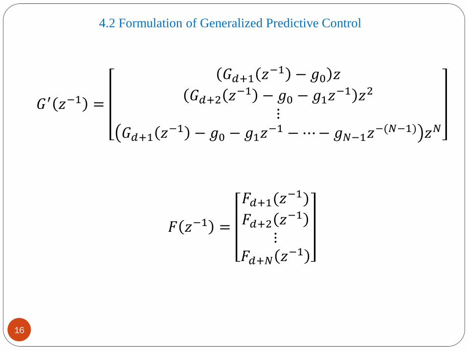
𝐺′ 𝑧−1 =
𝐺𝑑+1 𝑧−1 − 𝑔0 𝑧
𝐺𝑑+2 𝑧−1 − 𝑔0 − 𝑔1𝑧−1 𝑧2
⋮𝐺𝑑+1 𝑧−1 − 𝑔0 − 𝑔1𝑧
−1 − ⋯ − 𝑔𝑁−1𝑧−(𝑁−1) 𝑧𝑁
𝐹 𝑧−1 =
𝐹𝑑+1(𝑧−1)
𝐹𝑑+2 𝑧−1
⋮𝐹𝑑+𝑁 𝑧−1
16
4.2 Formulation of Generalized Predictive Control
• Notice that the last two terms in Equation (4.6)
• 𝐲 = 𝐆𝐮 + 𝐅 z−1 𝐲 t + 𝐆′ z−1 ∆𝑢 𝑡 − 1 (4.6)
• only depend on the past and can be grouped into 𝐟 leading
to:
𝐲 = 𝐆𝐮 + 𝐟
• Notice that if all initial conditions are zero, the free
response 𝐟 is also zero.
17
4.2 Formulation of Generalized Predictive Control
• If a unit step is applied to the input at time 𝑡; that is,
∆𝑢(𝑡) = 1, ∆𝑢(𝑡 + 1) = 0, . . . , ∆𝑢(𝑡 + 𝑁 − 1) = 0
• the expected output sequence:
𝑦 𝑡 + 1 , 𝑦 𝑡 + 2 , . . . , 𝑦 𝑡 + 𝑁 𝑇
• is equal to the first column of matrix 𝐺.
• That is, the first column of matrix 𝐺 can be calculated asthe step response of the plant when a unit step is applied tothe manipulated variable.
18
4.2 Formulation of Generalized Predictive Control
• The free response term can be calculated recursively by:
𝑓𝑗+1 = 𝑧 1 − 𝐴 𝑧−1 𝐟𝑗 + 𝐵(𝑧−1)∆𝑢(𝑡 − 𝑑 + 𝑗)
• with 𝐟0 = 𝑦(𝑡) and ∆𝑢(𝑡 + 𝑗) = 0 𝑓𝑜𝑟 𝑗 ≥ 0.
19
4.2 Formulation of Generalized Predictive Control
• Expression (4.2) can be written as:
𝐉 = 𝐆𝐮 + 𝐟 − 𝐰 T (𝐆𝐮 + 𝐟 − 𝐰) + λ𝐮T𝐮 (4.7)
• Where:
𝐰 = 𝑤 𝑡 + 𝑑 + 1 𝑤 𝑡 + 𝑑 + 2 · · · 𝑤 𝑡 + 𝑑 + 𝑁 𝑇
20
4.2 Formulation of Generalized Predictive Control
• Equation (4.7) can be written as:
𝑱 =1
2𝐮T𝐇𝐮 + 𝐛T𝐮 + 𝑓0 (4.8)
• Where:
𝑯 = 𝟐(𝑮𝑇𝑮 + 𝜆𝑰)
𝐛T = 2 𝐟 − 𝐰 T𝐆
𝑓0 = 𝐟 − 𝐰 T (𝐟 − 𝐰)
21
4.2 Formulation of Generalized Predictive Control
• The minimum of 𝑱, assuming there are no constraints on the
control signals, can be found by making the gradient of 𝑱equal to zero, which leads to:
𝐮 = −𝐇−1𝐛 = 𝐆T𝐆 + λ𝐈−1
𝐆T (𝐰 − 𝐟 ) (4.9)
• Notice that the control signal that is actually sent to the
process is the first element of vector 𝐮, given by:
∆𝑢 𝑡 = 𝐊 𝐰 − 𝐟 (4.10)
• Where 𝐾 is the first row of matrix 𝐆T𝐆 + λ𝐈−1
𝐆T .22
4.2 Formulation of Generalized Predictive Control
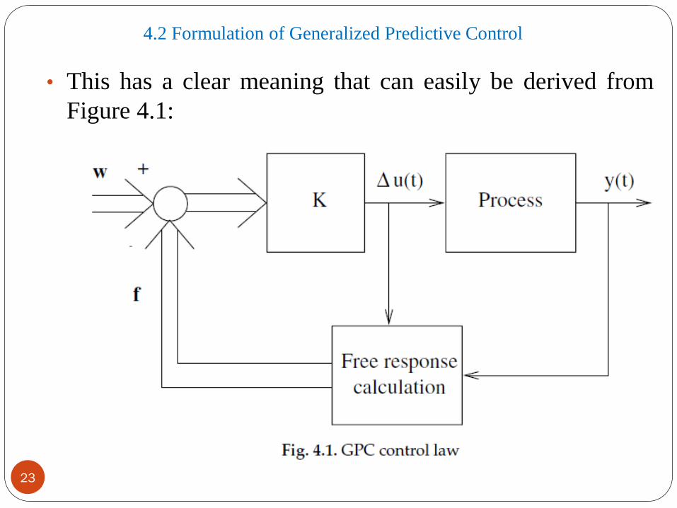
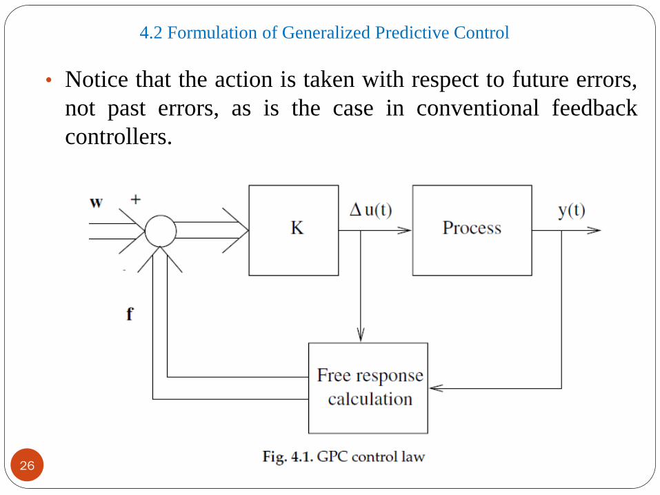
• This has a clear meaning that can easily be derived from
Figure 4.1:
23
4.2 Formulation of Generalized Predictive Control
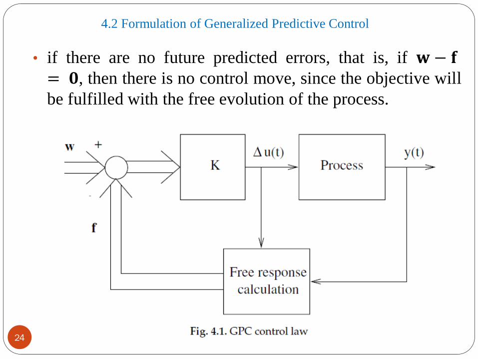
• if there are no future predicted errors, that is, if 𝐰 − 𝐟= 𝟎, then there is no control move, since the objective will
be fulfilled with the free evolution of the process.
24

4.2 Formulation of Generalized Predictive Control
• However, in the other case, there will be an increment in
the control action proportional (with a factor K) to that
future error.
25
4.2 Formulation of Generalized Predictive Control
• Notice that the action is taken with respect to future errors,
not past errors, as is the case in conventional feedback
controllers.
26
4.2 Formulation of Generalized Predictive Control
• Notice that only the first element of 𝐮is applied and the
procedure is repeated at the next sampling time.
• The solution to the GPC given involves the inversion (or
triangularization) of an 𝑁 × 𝑁 matrix which requires a
substantial amount of computation.
27

4.2 Formulation of Generalized Predictive Control
• In [58] the concept of control horizon is used to reduce the
amount of computation needed, assuming that the projected
control signals are going to be constant after 𝑁𝑢 < 𝑁.
• This leads to the inversion of an 𝑁𝑢 × 𝑁𝑢 matrix which
reduces the amount of computation (in particular, if 𝑁𝑢
= 1 it is reduced to a scalar computation, as in EPSAC),
but restricts the optimality of the GPC.
28

4.4 An Example
29
4.4 An Example
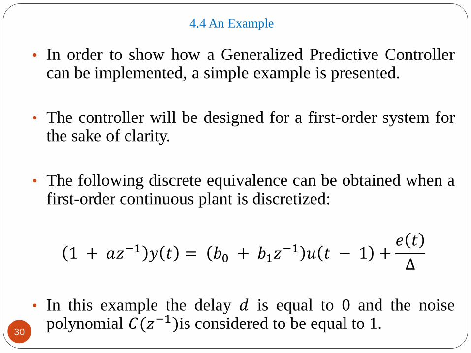
• In order to show how a Generalized Predictive Controllercan be implemented, a simple example is presented.
• The controller will be designed for a first-order system forthe sake of clarity.
• The following discrete equivalence can be obtained when afirst-order continuous plant is discretized:
1 + 𝑎𝑧−1 𝑦 𝑡 = 𝑏0 + 𝑏1𝑧−1 𝑢 𝑡 − 1 +𝑒 𝑡
∆
• In this example the delay 𝑑 is equal to 0 and the noisepolynomial 𝐶(𝑧−1)is considered to be equal to 1.
30
4.4 An Example
• The algorithm to obtain the control law described in the
previous section will be used on the preceding system,
obtaining numerical results for the parameter values 𝑎= −0.8, 𝑏0 = 0.4 and 𝑏1 = 0.6, the horizons being 𝑁1
= 1and 𝑁2 = 𝑁𝑢 = 3.
• As has been shown, predicted values of the process output
over the horizon are first calculated and rewritten in the
form of Equation (4.6), and then the control law is
computed using Expression (4.9).
31
4.4 An Example
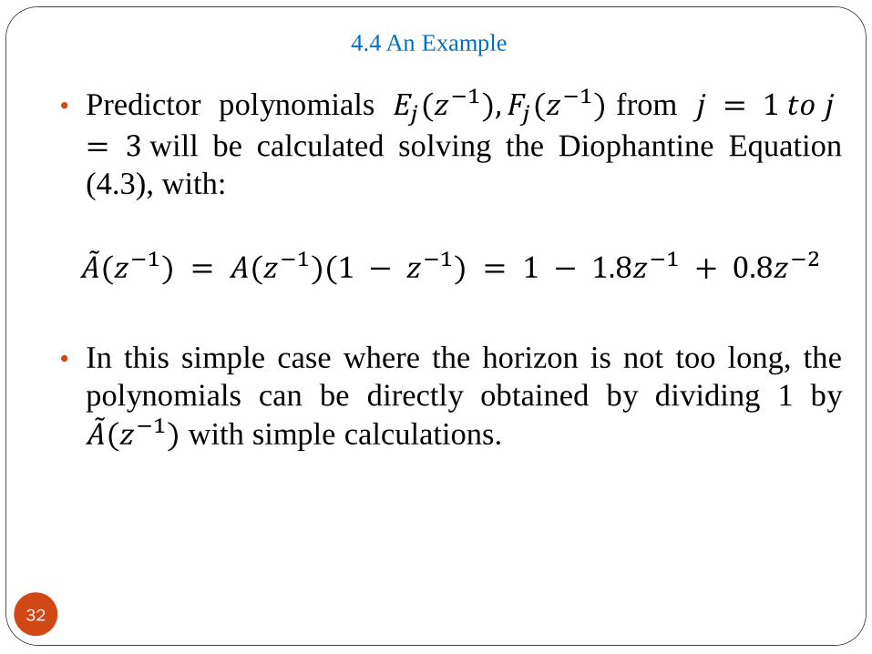
• Predictor polynomials 𝐸𝑗(𝑧−1), 𝐹𝑗(𝑧
−1) from 𝑗 = 1 𝑡𝑜 𝑗
= 3 will be calculated solving the Diophantine Equation
(4.3), with:
𝐴(𝑧−1) = 𝐴(𝑧−1)(1 − 𝑧−1) = 1 − 1.8𝑧−1 + 0.8𝑧−2
• In this simple case where the horizon is not too long, the
polynomials can be directly obtained by dividing 1 by 𝐴(𝑧−1) with simple calculations.
32
33
4.4 An Example
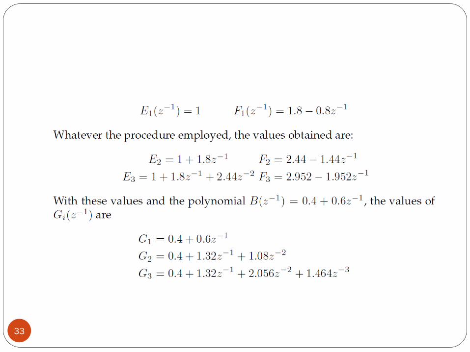
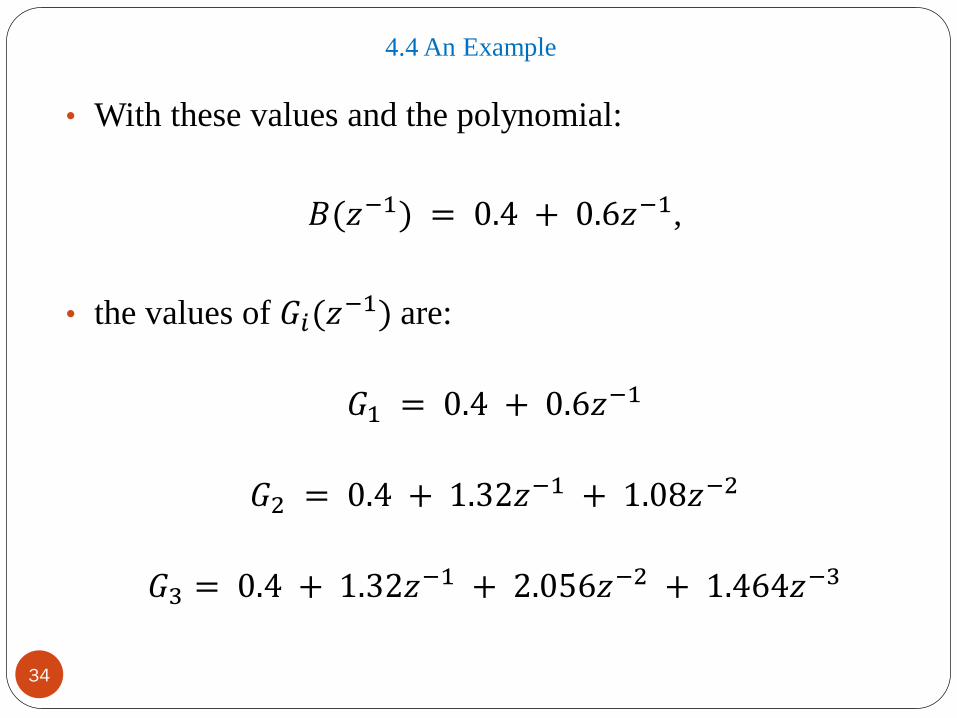
• With these values and the polynomial:
𝐵(𝑧−1) = 0.4 + 0.6𝑧−1,
• the values of 𝐺𝑖(𝑧−1) are:
𝐺1 = 0.4 + 0.6𝑧−1
𝐺2 = 0.4 + 1.32𝑧−1 + 1.08𝑧−2
𝐺3 = 0.4 + 1.32𝑧−1 + 2.056𝑧−2 + 1.464𝑧−3
34
4.4 An Example
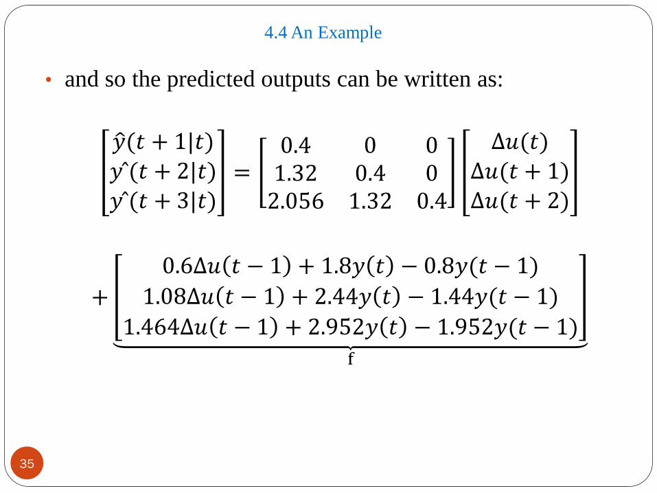
• and so the predicted outputs can be written as:
𝑦(𝑡 + 1|𝑡)
𝑦 ̂(𝑡 + 2|𝑡)𝑦 ̂(𝑡 + 3|𝑡)
=0.4 0 01.32 0.4 02.056 1.32 0.4
∆𝑢(𝑡)
∆𝑢(𝑡 + 1)∆𝑢(𝑡 + 2)
+
0.6∆𝑢 𝑡 − 1 + 1.8𝑦 𝑡 − 0.8𝑦(𝑡 − 1)
1.08∆𝑢 𝑡 − 1 + 2.44𝑦 𝑡 − 1.44𝑦(𝑡 − 1)
1.464∆𝑢 𝑡 − 1 + 2.952𝑦 𝑡 − 1.952𝑦(𝑡 − 1)
f
35
4.4 An Example
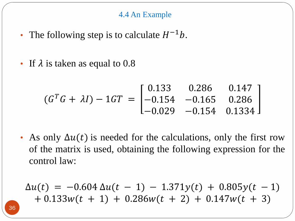
• The following step is to calculate 𝐻−1𝑏.
• If 𝜆 is taken as equal to 0.8
(𝐺𝑇𝐺 + 𝜆𝐼) − 1𝐺𝑇 =0.133 0.286 0.147
−0.154 −0.165 0.286−0.029 −0.154 0.1334
• As only ∆𝑢(𝑡) is needed for the calculations, only the first row
of the matrix is used, obtaining the following expression for the
control law:
∆𝑢(𝑡) = −0.604 ∆𝑢(𝑡 − 1) − 1.371𝑦(𝑡) + 0.805𝑦(𝑡 − 1)+ 0.133𝑤(𝑡 + 1) + 0.286𝑤(𝑡 + 2) + 0.147𝑤(𝑡 + 3)
36
4.4 An Example
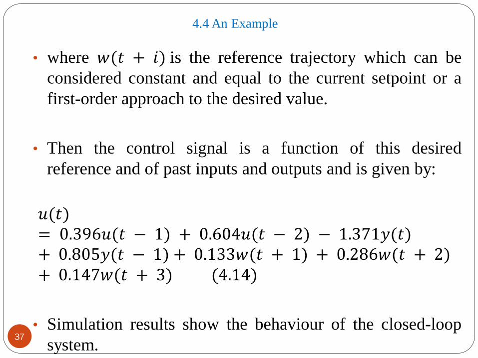
• where 𝑤(𝑡 + 𝑖) is the reference trajectory which can be
considered constant and equal to the current setpoint or a
first-order approach to the desired value.
• Then the control signal is a function of this desired
reference and of past inputs and outputs and is given by:
𝑢(𝑡)= 0.396𝑢(𝑡 − 1) + 0.604𝑢(𝑡 − 2) − 1.371𝑦(𝑡)+ 0.805𝑦(𝑡 − 1) + 0.133𝑤(𝑡 + 1) + 0.286𝑤(𝑡 + 2)+ 0.147𝑤(𝑡 + 3) (4.14)
• Simulation results show the behaviour of the closed-loop
system.37
4.4 An Example
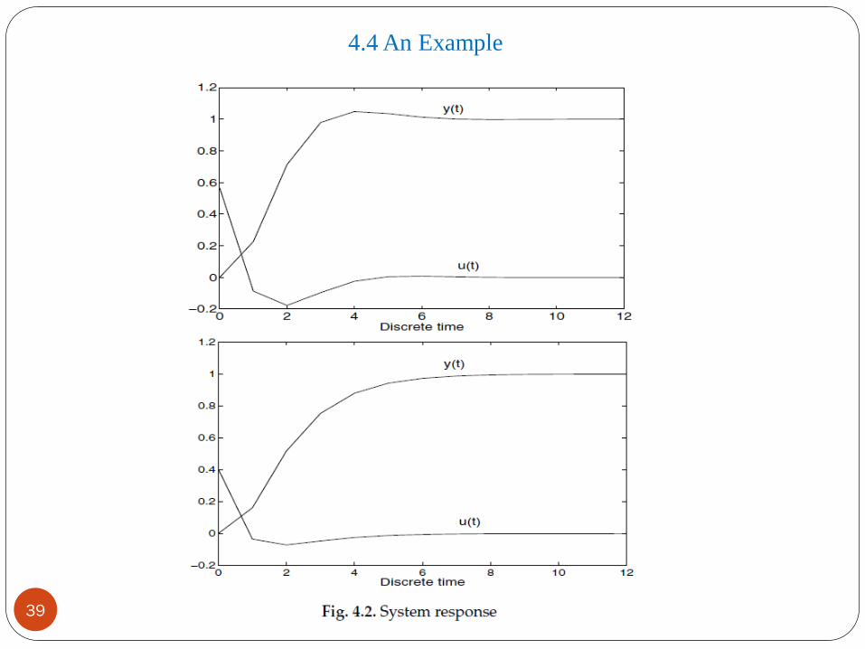
• In the first graph of Figure 4.2 the reference is constant and
equal to 1, and in the second one there is a smooth
approach to the same value, obtaining a slightly different
response, slower but without overshoot.
38
4.4 An Example
39
4.4 An Example
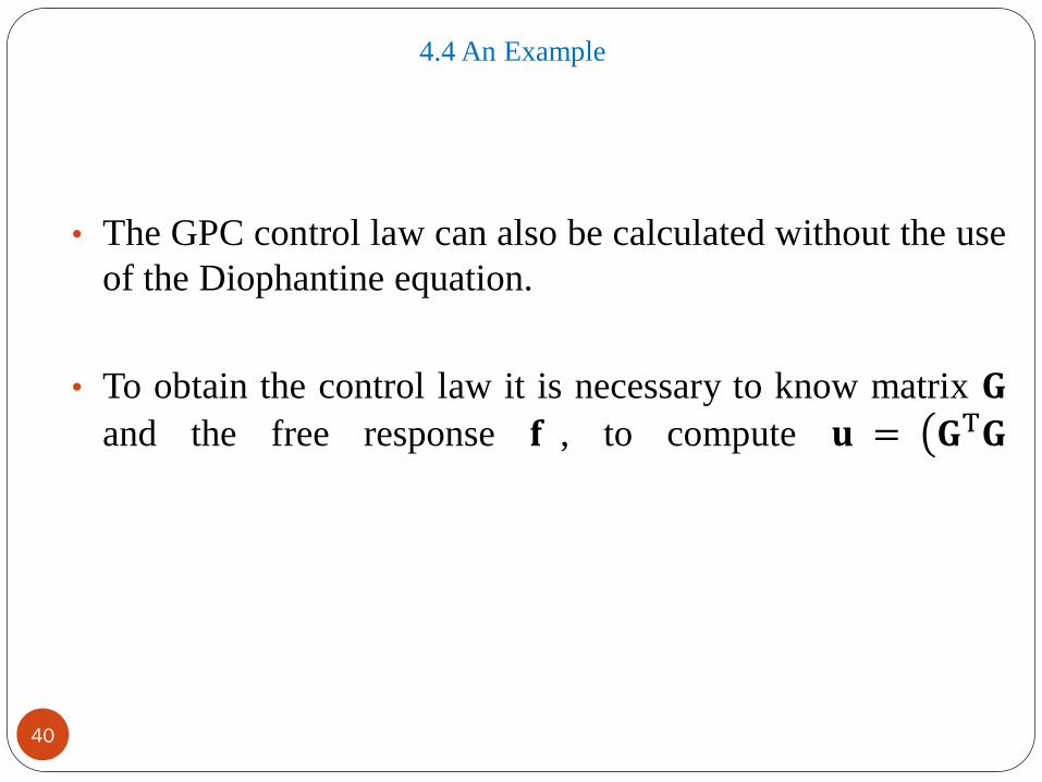
• The GPC control law can also be calculated without the use
of the Diophantine equation.
• To obtain the control law it is necessary to know matrix 𝐆
and the free response 𝐟 , to compute 𝐮 = 𝐆T𝐆
40
4.4 An Example
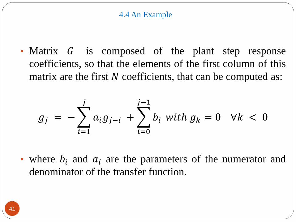
• Matrix 𝐺 is composed of the plant step response
coefficients, so that the elements of the first column of this
matrix are the first 𝑁 coefficients, that can be computed as:
𝑔𝑗 = −
𝑖=1
𝑗
𝑎𝑖𝑔𝑗−𝑖 +
𝑖=0
𝑗−1
𝑏𝑖 𝑤𝑖𝑡ℎ 𝑔𝑘 = 0 ∀𝑘 < 0
• where 𝑏𝑖 and 𝑎𝑖 are the parameters of the numerator and
denominator of the transfer function.
41
4.4 An Example
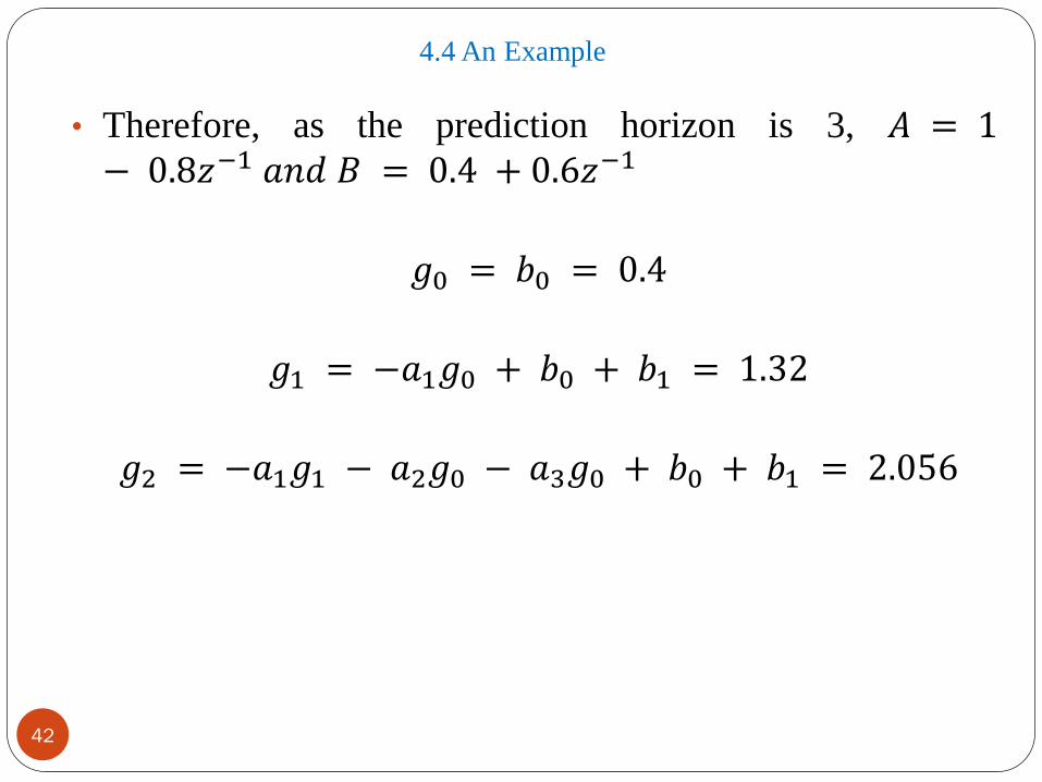
• Therefore, as the prediction horizon is 3, 𝐴 = 1− 0.8𝑧−1 𝑎𝑛𝑑 𝐵 = 0.4 + 0.6𝑧−1
𝑔0 = 𝑏0 = 0.4
𝑔1 = −𝑎1𝑔0 + 𝑏0 + 𝑏1 = 1.32
𝑔2 = −𝑎1𝑔1 − 𝑎2𝑔0 − 𝑎3𝑔0 + 𝑏0 + 𝑏1 = 2.056
42
4.4 An Example
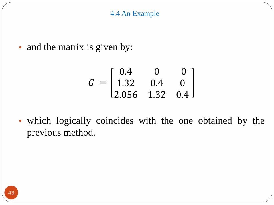
• and the matrix is given by:
𝐺 =0.4 0 01.32 0.4 02.056 1.32 0.4
• which logically coincides with the one obtained by the
previous method.
43
4.4 An Example
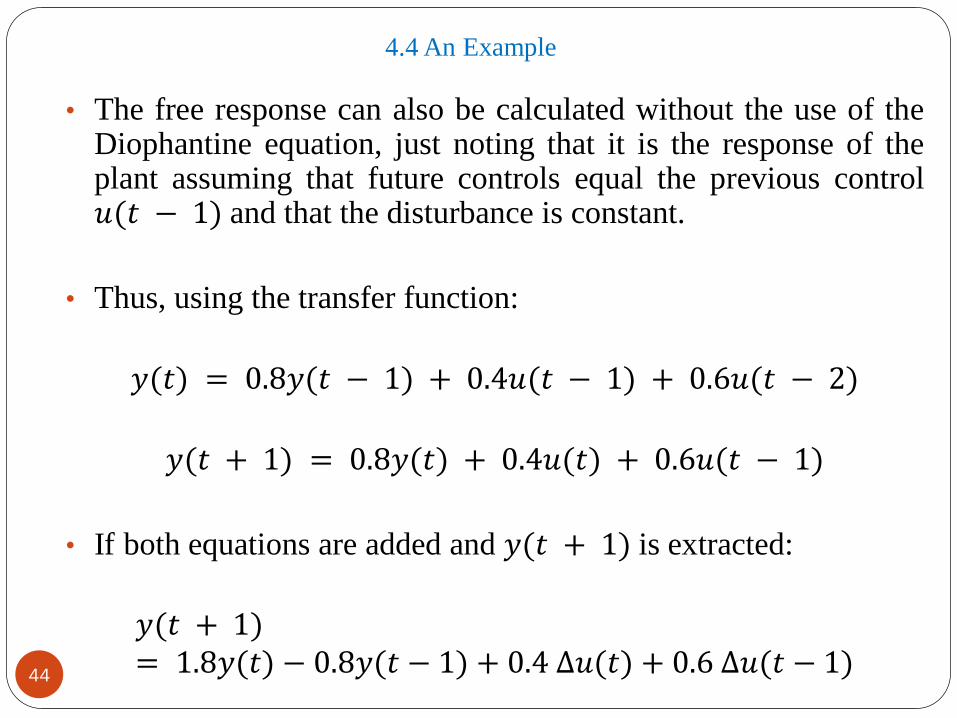
• The free response can also be calculated without the use of theDiophantine equation, just noting that it is the response of theplant assuming that future controls equal the previous control𝑢(𝑡 − 1) and that the disturbance is constant.
• Thus, using the transfer function:
𝑦(𝑡) = 0.8𝑦(𝑡 − 1) + 0.4𝑢(𝑡 − 1) + 0.6𝑢(𝑡 − 2)
𝑦(𝑡 + 1) = 0.8𝑦(𝑡) + 0.4𝑢(𝑡) + 0.6𝑢(𝑡 − 1)
• If both equations are added and 𝑦(𝑡 + 1) is extracted:
𝑦(𝑡 + 1)= 1.8𝑦(𝑡) − 0.8𝑦(𝑡 − 1) + 0.4 ∆𝑢(𝑡) + 0.6 ∆𝑢(𝑡 − 1)
44
4.4 An Example
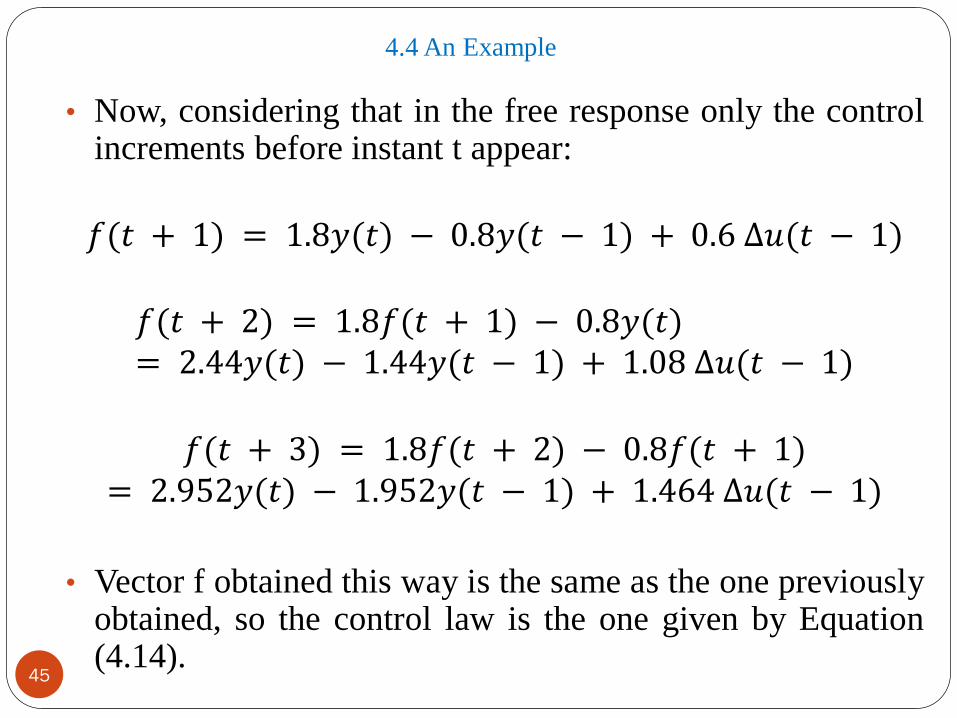
• Now, considering that in the free response only the controlincrements before instant t appear:
𝑓(𝑡 + 1) = 1.8𝑦(𝑡) − 0.8𝑦(𝑡 − 1) + 0.6 ∆𝑢(𝑡 − 1)
𝑓(𝑡 + 2) = 1.8𝑓(𝑡 + 1) − 0.8𝑦(𝑡)= 2.44𝑦(𝑡) − 1.44𝑦(𝑡 − 1) + 1.08 ∆𝑢(𝑡 − 1)
𝑓(𝑡 + 3) = 1.8𝑓(𝑡 + 2) − 0.8𝑓(𝑡 + 1)= 2.952𝑦(𝑡) − 1.952𝑦(𝑡 − 1) + 1.464 ∆𝑢(𝑡 − 1)
• Vector f obtained this way is the same as the one previouslyobtained, so the control law is the one given by Equation(4.14).
45

4.3 The Coloured Noise Case
46
4.3 The Coloured Noise Case
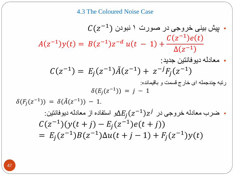
𝐶(𝑧−1)نبودن1صورتدرخروجیبینیپیش•
𝐴 𝑧−1 𝑦 𝑡 = 𝐵 𝑧−1 𝑧−𝑑 𝑢 𝑡 − 1 +𝐶 𝑧−1 𝑒 𝑡
∆ 𝑧−1
:جدیددیوفانتینمعادله•
𝐶 𝑧−1 = 𝐸𝑗 𝑧−1 𝐴 𝑧−1 + 𝑧−𝑗𝐹𝑗 𝑧−1
:رتبه چندجمله ای خارج قسمت و باقیمانده
𝛿(𝐸𝑗(𝑧−1)) = 𝑗 − 1
𝛿(𝐹𝑗(𝑧−1)) = 𝛿( 𝐴(𝑧−1)) − 1.
𝐸𝑗∆ضرب معادله خروجی در • 𝑧−1 𝑧𝑗و استفاده از معادله دیوفانتین:
𝐶(𝑧−1)(𝑦(𝑡 + 𝑗) − 𝐸𝑗(𝑧−1)𝑒(𝑡 + 𝑗))
= 𝐸𝑗(𝑧−1)𝐵(𝑧−1)∆𝑢(𝑡 + 𝑗 − 1) + 𝐹𝑗(𝑧
−1)𝑦(𝑡)
47
4.3 The Coloured Noise Case
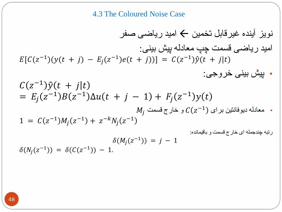
امید ریاضی صفرنویز آینده غیرقابل تخمین
:امید ریاضی قسمت چپ معادله پیش بینی𝐸[𝐶(𝑧−1)(𝑦(𝑡 + 𝑗) − 𝐸𝑗(𝑧
−1)𝑒(𝑡 + 𝑗))] = 𝐶(𝑧−1) 𝑦(𝑡 + 𝑗|𝑡)
:پیش بینی خروجی•
𝐶 𝑧−1 𝑦 𝑡 + 𝑗 𝑡= 𝐸𝑗 𝑧−1 𝐵 𝑧−1 ∆𝑢 𝑡 + 𝑗 − 1 + 𝐹𝑗 𝑧−1 𝑦 𝑡
𝐶برایدیوفانتینمعادله• 𝑧−1قسمتخارجو𝑀𝑗
1 = 𝐶 𝑧−1 𝑀𝑗 𝑧−1 + 𝑧−𝑘𝑁𝑗 𝑧−1
:رتبه چندجمله ای خارج قسمت و باقیمانده
𝛿(𝑀𝑗(𝑧−1)) = 𝑗 − 1
𝛿(𝑁𝑗(𝑧−1)) = 𝛿(𝐶(𝑧−1)) − 1.
48
4.3 The Coloured Noise Case
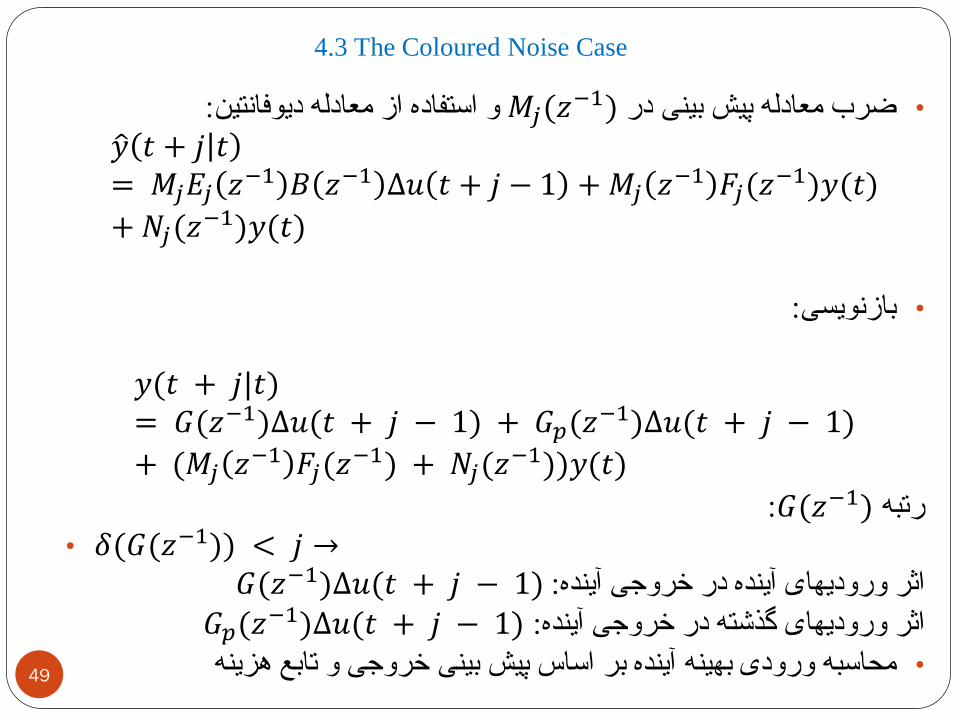
𝑀𝑗(𝑧دربینیپیشمعادلهضرب•:دیوفانتینمعادلهازاستفادهو(1−
𝑦 𝑡 + 𝑗 𝑡= 𝑀𝑗𝐸𝑗 𝑧−1 𝐵 𝑧−1 ∆𝑢 𝑡 + 𝑗 − 1 + 𝑀𝑗 𝑧−1 𝐹𝑗(𝑧
−1)𝑦(𝑡)
+ 𝑁𝑗(𝑧−1)𝑦(𝑡)
:بازنویسی•
𝑦(𝑡 + 𝑗|𝑡)= 𝐺(𝑧−1)∆𝑢(𝑡 + 𝑗 − 1) + 𝐺𝑝(𝑧−1)∆𝑢(𝑡 + 𝑗 − 1)
+ (𝑀𝑗 𝑧−1 𝐹𝑗(𝑧−1) + 𝑁𝑗(𝑧
−1))𝑦(𝑡)
:𝐺(𝑧−1)رتبه
• 𝛿(𝐺(𝑧−1)) < 𝑗 →𝐺(𝑧−1)∆𝑢(𝑡:آیندهخروجیدرآیندهورودیهایاثر + 𝑗 − 1)𝐺𝑝(𝑧−1)∆𝑢(𝑡:آیندهخروجیدرگذشتهورودیهایاثر + 𝑗 − 1)
49هزینهتابعوخروجیبینیپیشاساسبرآیندهبهینهورودیمحاسبه•
4.3 The Coloured Noise Case
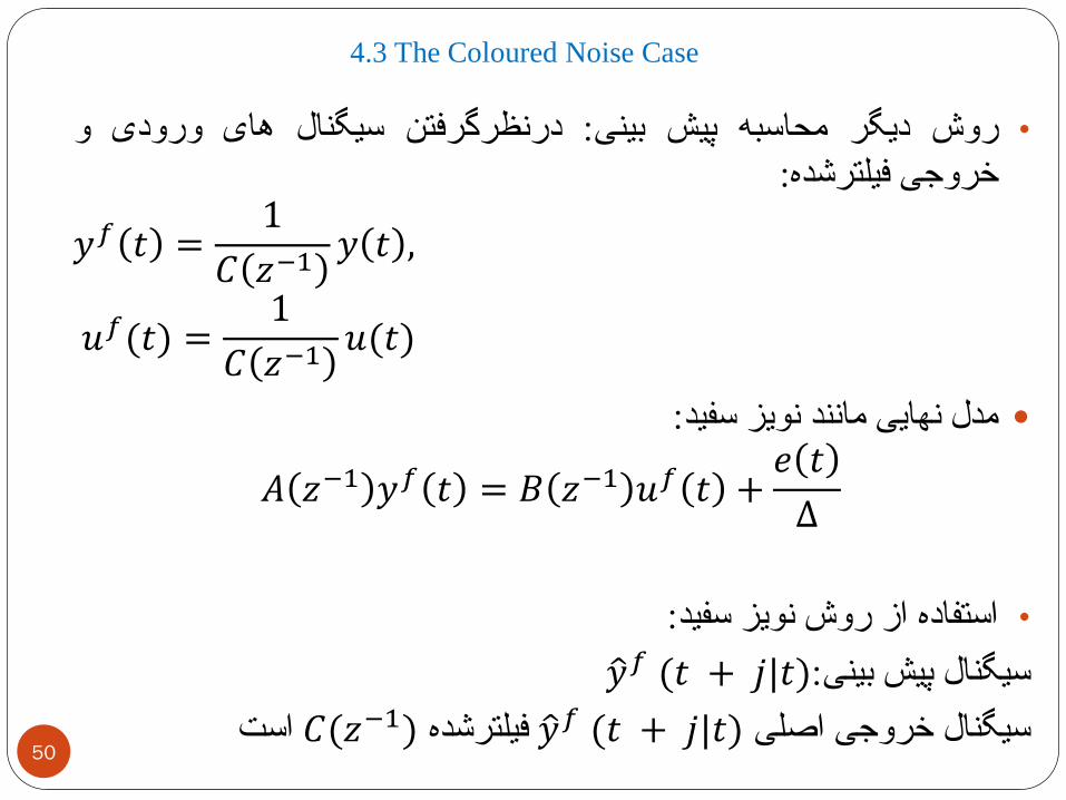
وورودیهایسیگنالدرنظرگرفتن:بینیپیشمحاسبهدیگرروش•
:فیلترشدهخروجی
𝑦𝑓 𝑡 =1
𝐶 𝑧−1𝑦 𝑡 ,
𝑢𝑓(𝑡) =1
𝐶 𝑧−1𝑢(𝑡)
مدل نهایی مانند نویز سفید:
𝐴 𝑧−1 𝑦𝑓 𝑡 = 𝐵 𝑧−1 𝑢𝑓 𝑡 +𝑒 𝑡
∆
:استفاده از روش نویز سفید•
𝑦𝑓 :سیگنال پیش بینی (𝑡 + 𝑗|𝑡)
𝑦𝑓 سیگنال خروجی اصلی (𝑡 + 𝑗|𝑡) فیلترشده𝐶(𝑧−1)است50