chapter 8 competition and coexistence
DESCRIPTION
Chapter 8 Competition and Coexistence. 群體生態學 Synecology: community ecology. 以生物組織水準來分 個體生態學 Autecology: Life history, adaptation 種群生態學 Population ecology 群體生態學 Synecology: community ecology 生態系統生態學 Ecosystem ecology. Outline. Forms of competition: Interspecific and intraspecific - PowerPoint PPT PresentationTRANSCRIPT
Chapter 8Competition
and Coexistence
群體生態學 Synecology: community ecology
以生物組織水準來分1.個體生態學 Autecology: Life history,
adaptation
2.種群生態學 Population ecology
3.群體生態學 Synecology: community ecology
4.生態系統生態學 Ecosystem ecology
Outline• Forms of competition: Interspecific and
intraspecific• Intraspecific competition
– Common in nature– Described by the 3/2 thinning law
Outline• Interspecific competition
– Common in nature– Outcome affected by
• Physical environment• Other species
Outline• Competition
– Exists among 55-75% of the species– Mechanism: over use of the same resource
Outline• Mathematical models, called Lotka-
Volterra models, predict four outcomes of competition– One species eliminated– The other species is eliminated– Both species coexist– Either species is eliminated, depending on
starting conditions
Outline• Competing species can coexist through
partitioning of resources

Community :群體,群聚,群落
• 群落是居住的相當靠近且有交互作用可能物種集合
• 生物在自然界依循一定的規律而集合成群落
• 特定空間或特定生境下若干生物種群有規律的組合
• 彼此間或與環境間互相作用與影響,具有一定形態結構與營養結構,執行一定功能
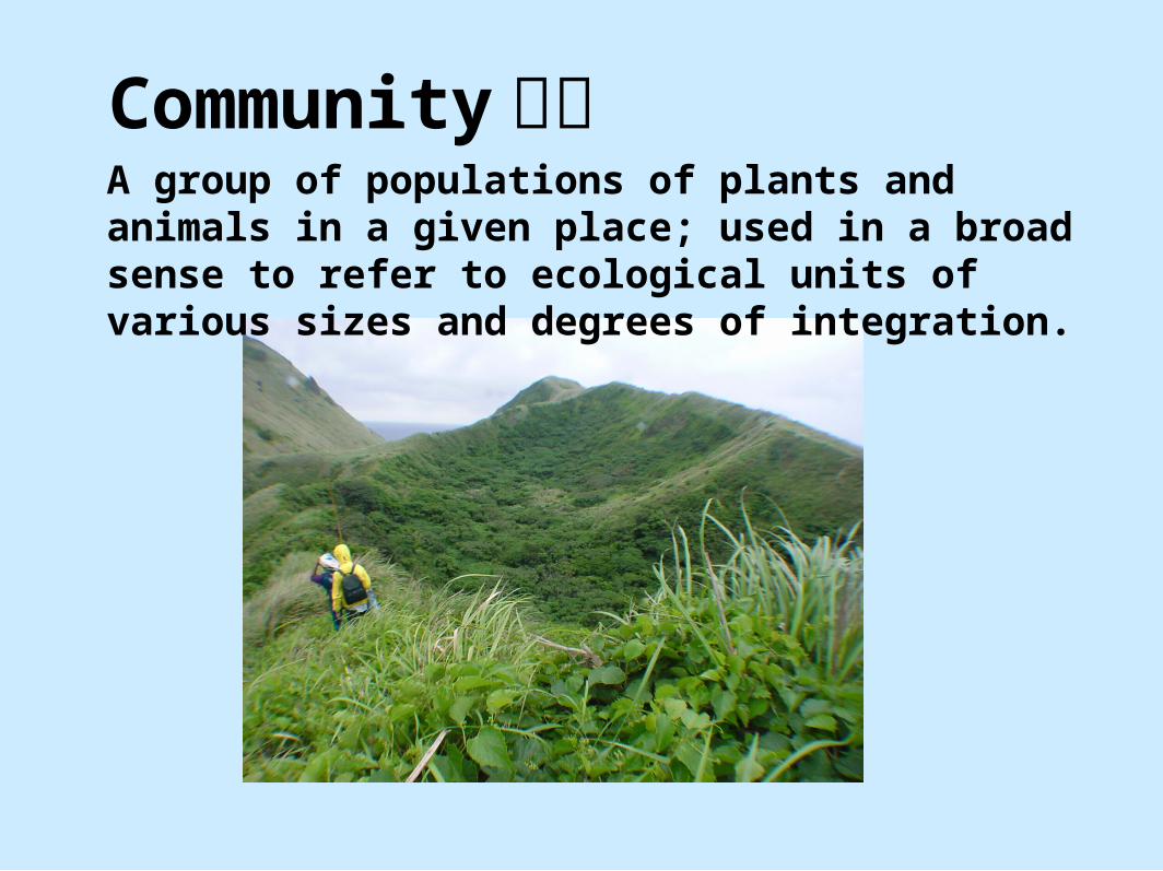
Community 群落 A group of populations of plants and animals in a given place; used in a broad sense to refer to ecological units of various sizes and degrees of integration.

福壽螺為什麼要把卵產在枝幹上?
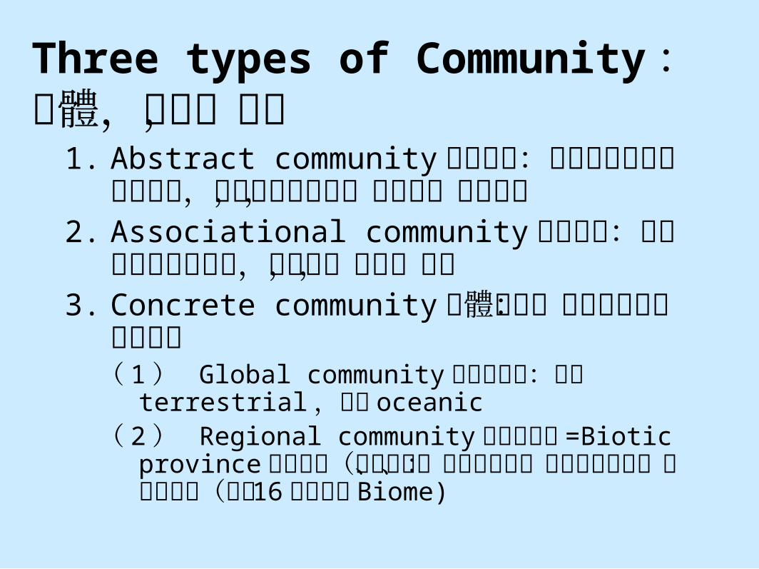
Three types of Community :群體,群聚,群落
1. Abstract community 抽象群聚:心裡想像的特殊形式群聚,事實上並不存在,如沙漠,草原群聚
2. Associational community 聯合群聚:過渡形式的生物群聚,如森林,草原,池塘
3. Concrete community 具體群聚:可直接觀察的特殊區域( 1 ) Global community 全球性群聚:陸地
terrestrial ,海洋 oceanic( 2 ) Regional community 區域性群聚 =Biotic
province 生物領域(根據溫度、雨量等不同、將全世界分成:冷溫熱三區(下含 16 個生物相 Biome)
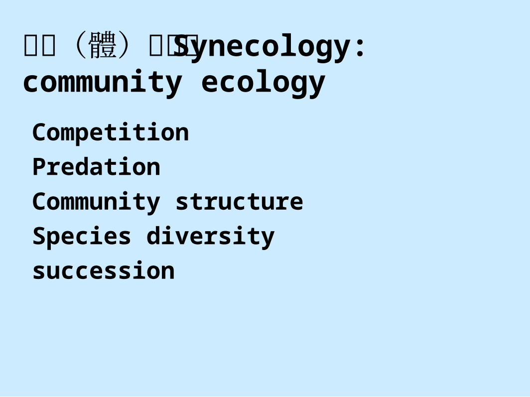
群落(體)生態學 Synecology: community ecology
Competition
Predation
Community structure
Species diversity
succession

群落的基本特徵
1.具有一定種類組成2.不同物種間相互影響3.形成群落環境4.具有一定結構5.一定的動態形式6.一定的分布範圍7.群落的邊界特徵
#14Chapt. 08
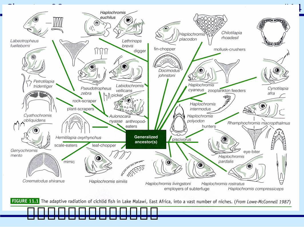
馬拉威湖慈鯛科的適應性演化
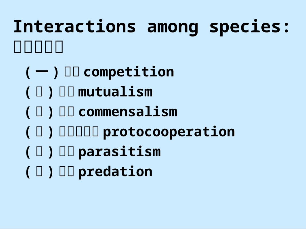
Interactions among species:種間的關係
( 一 ) 競爭 competition
( 二 ) 互惠 mutualism
( 三 ) 共棲 commensalism
( 四 ) 共生和附生 protocooperation
( 五 ) 寄生 parasitism
( 六 ) 捕食 predation
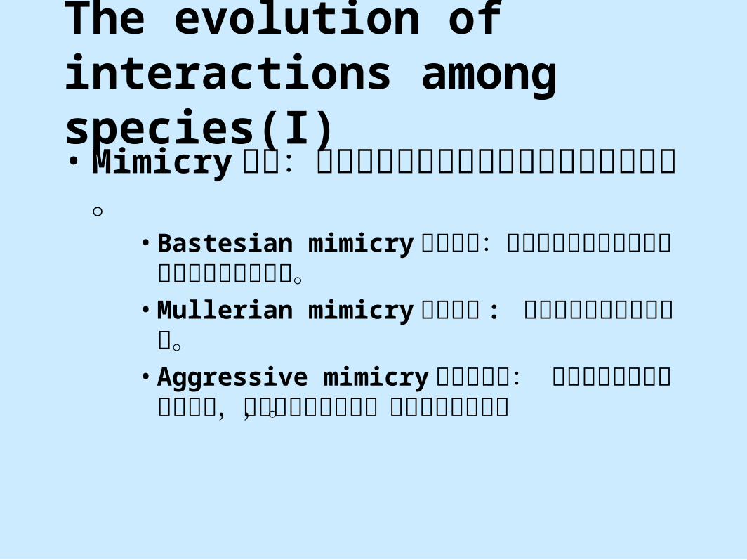
The evolution of interactions among species(I)• Mimicry 擬態:從模仿其他物種的外表上獲得好處的現象。
• Bastesian mimicry 貝氏擬態:無毒害的物種藉由模擬有害物種而獲利的情形。
• Mullerian mimicry 木氏擬態 : 兩種不同物種之間的擬態。
• Aggressive mimicry 攻擊性擬態: 有毒的種類模擬無毒的種類,以提升其偽裝效果,增加掠食成功率。
The evolution of interactions among species(II)• Coevolution 共同演化:例如植物和昆蟲間的共同演化。
• Parasitism 寄生 :
• Mutualism 互利共生:• Competition 競爭:• Predator-prey 掠食者與獵物:• Herbivore-plant 草食性動物與植物:
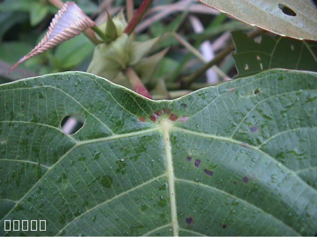
血桐的蜜線

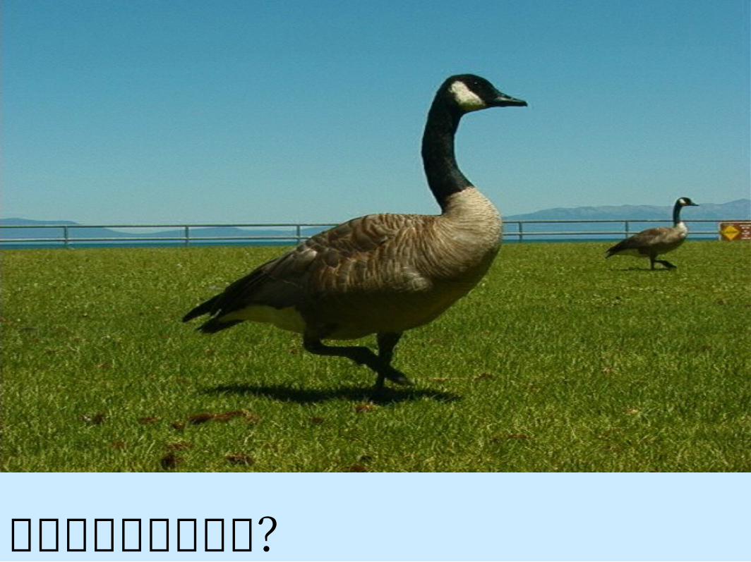
Why are community interactions important?
• 群體是居住的相當靠近且有交互作用可能物種集合
• 烏頭翁和白頭翁混居的結果會如何?• 草原上只有羚羊而沒有獅子,結果會如何?
• 如果沒有蝴蝶或蜜蜂,開花植物的世界將會如何?
動物可以消滅植物嗎?
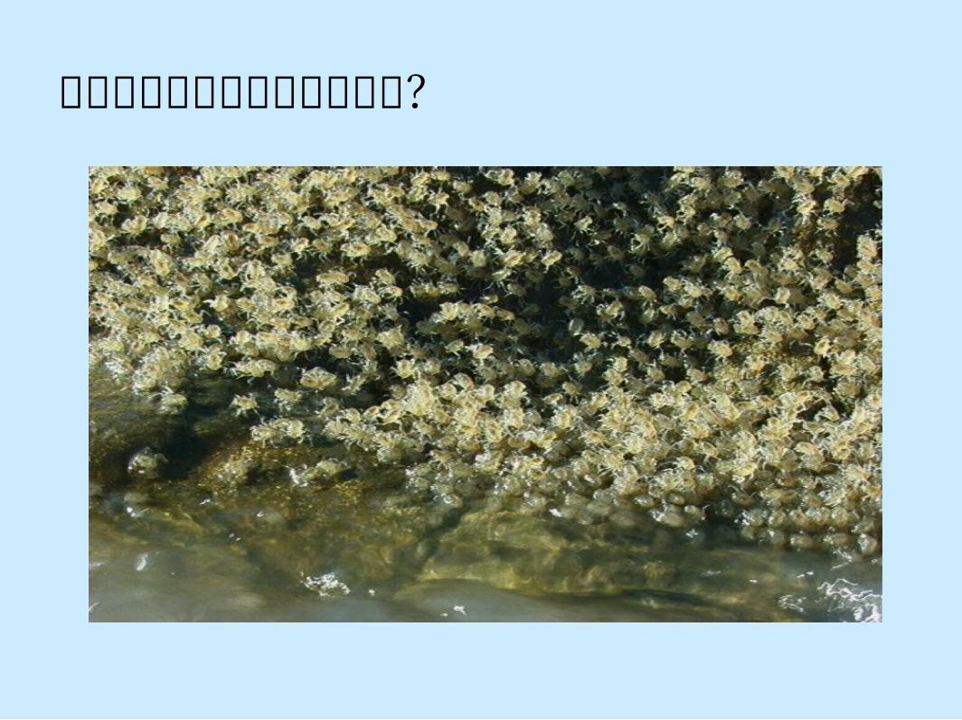
這麼多的小螃蟹都可以長大嗎?
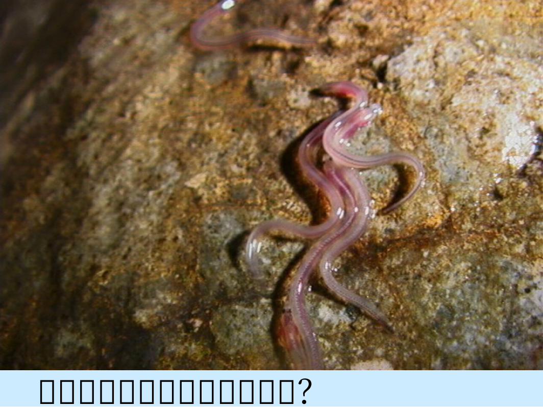
這些小鰻苗為什麼要力爭上游?
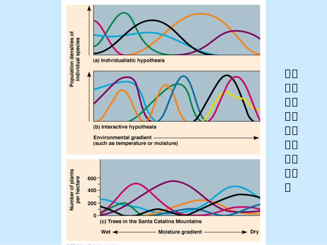
群聚的利己主義與交互作用假設的檢驗
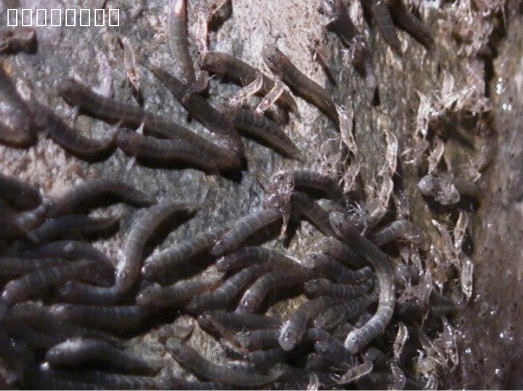
日本禿頭鯊和蝦苗

小蘭嶼火山口
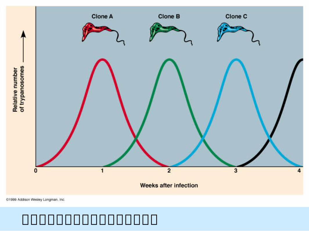
在寄主與寄生系統中快速的族群改變
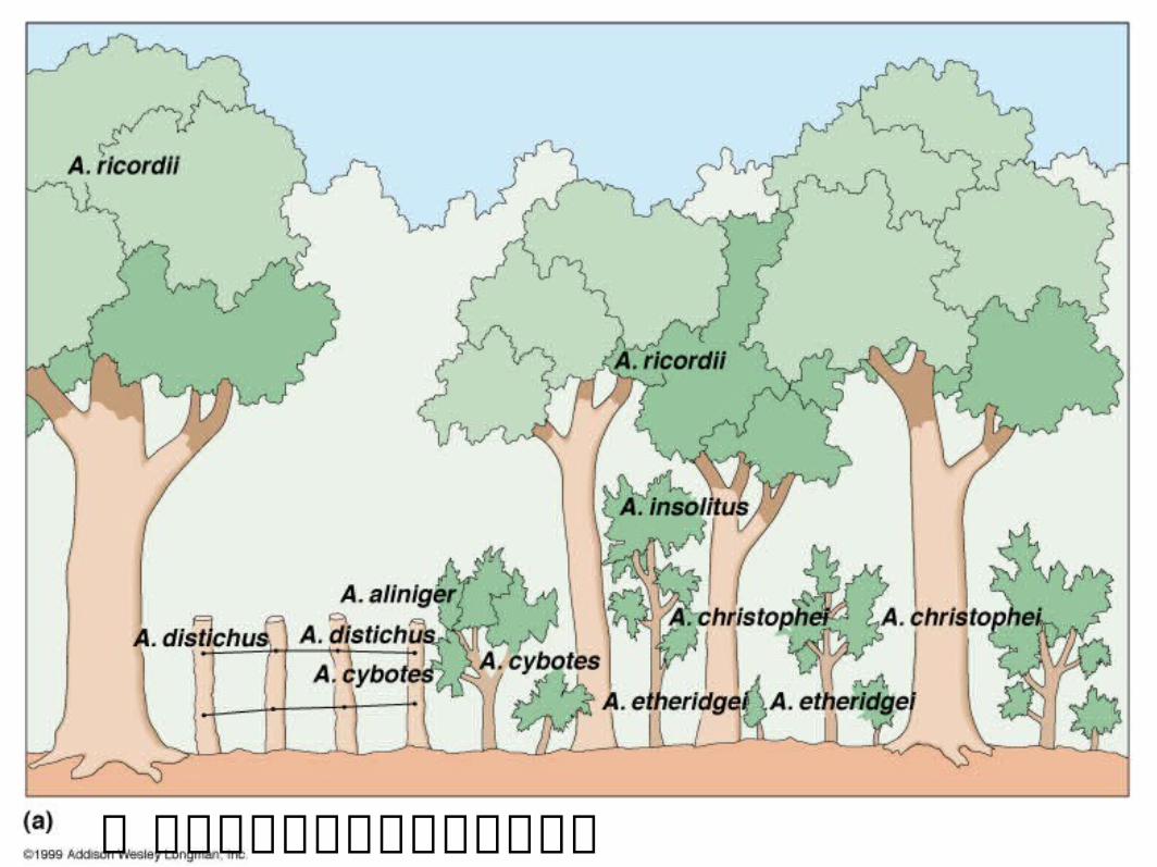
一群共域棲息蜥蜴的資源分配現象
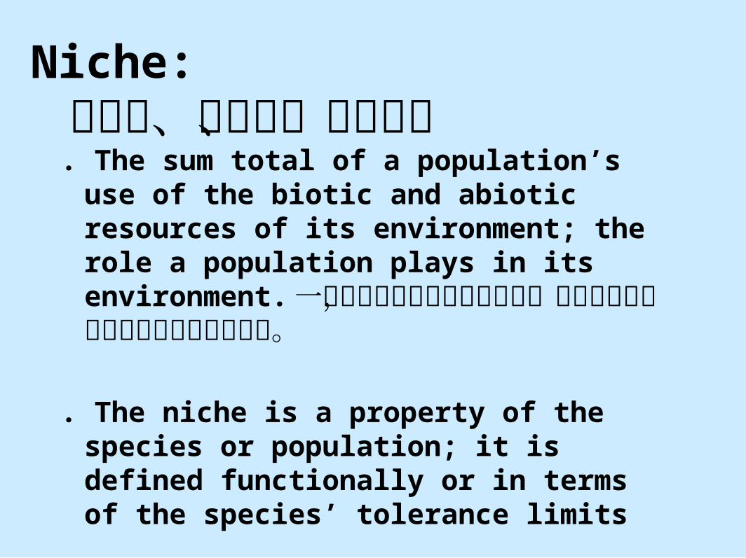
Niche: 生態龕、生態位、生態區位
. The sum total of a population’s use of the biotic and abiotic resources of its environment; the role a population plays in its environment. 一個生物在它所生存的環境中,對於生物性與非生物性資源利用的總和。
. The niche is a property of the species or population; it is defined functionally or in terms of the species’ tolerance limits
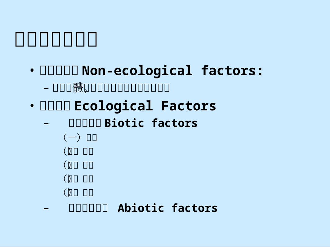
影響生物的因子• 非生態因子 Non-ecological factors:
– 對有機體生活無明顯影響的環境因子。• 生態因子 Ecological Factors
– 生物性因子 Biotic factors(一)共生(二)天敵(三)競爭(四)抑制(五)傳播
– 非生物性因子 Abiotic factors
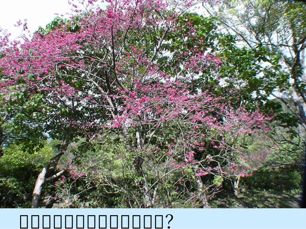
山櫻花為什麼先開花後長葉子?
自然競爭的實驗性證據
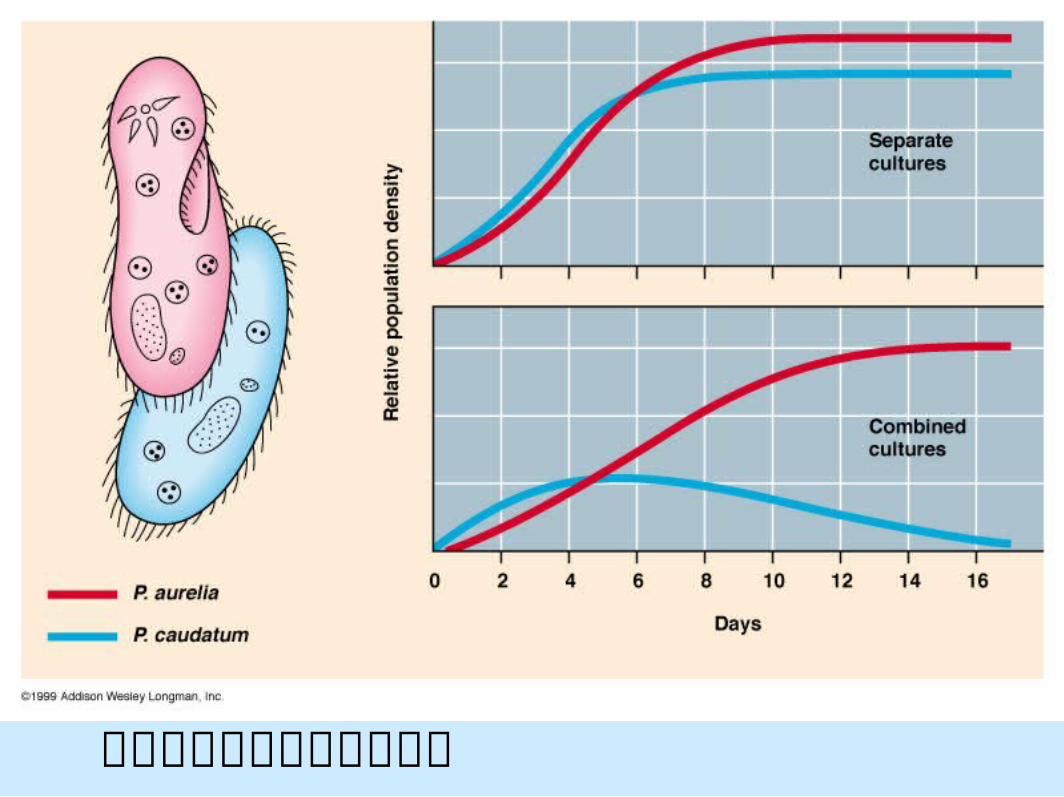
實驗室中草履蟲族群的競爭
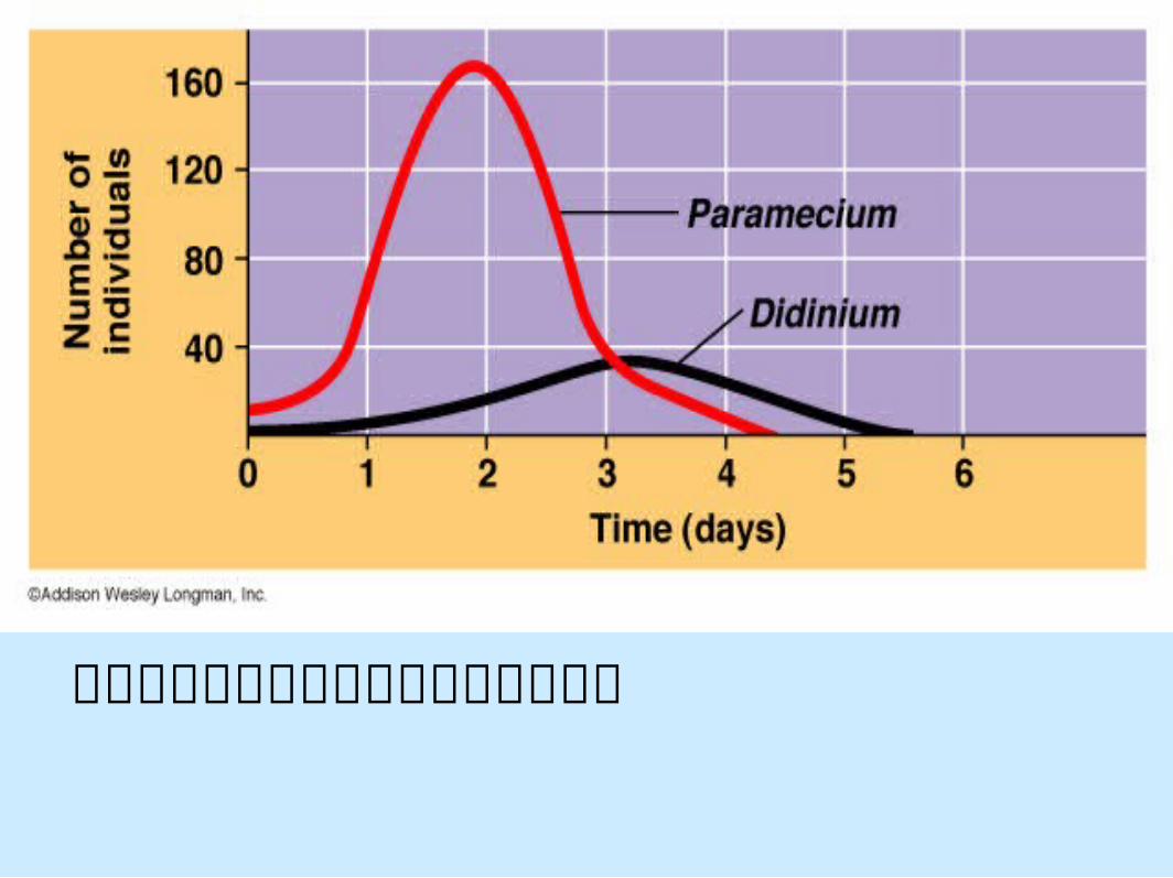
實驗室中掠食者和獵物之間的動態關係
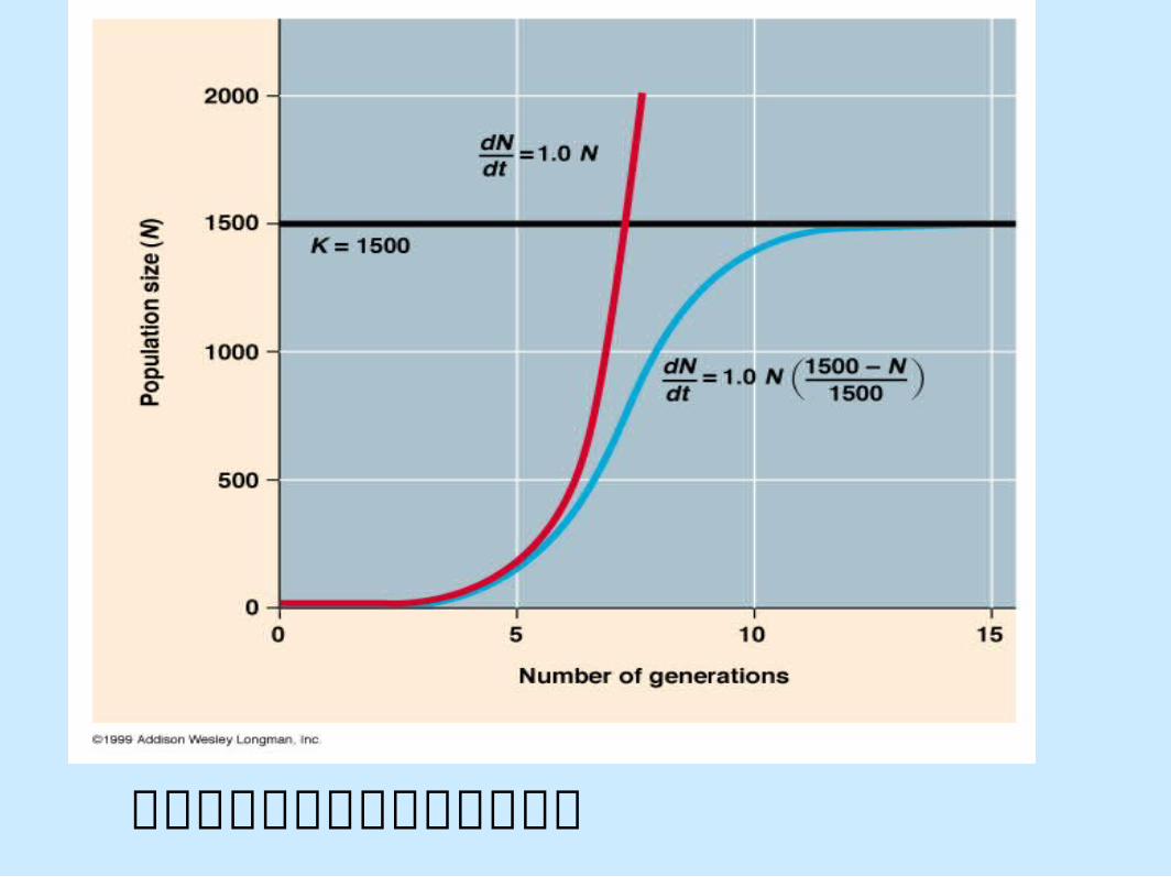
邏輯模型所預測的族群成長情形
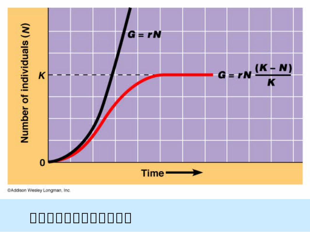
指數成長和對數成長的比較
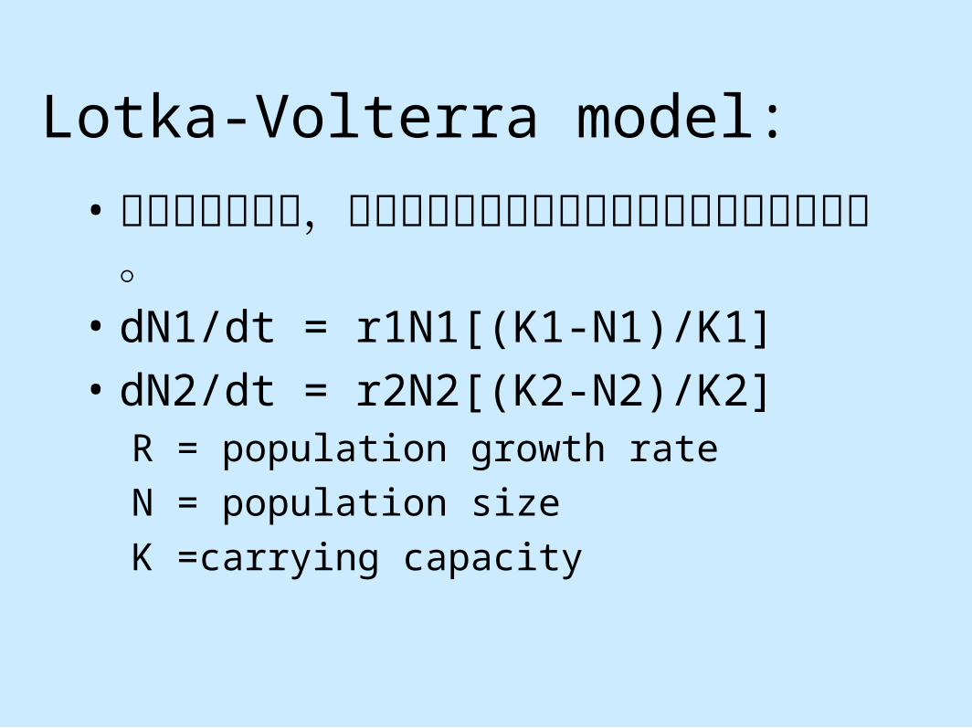
Lotka-Volterra model:
• 獵物按指數增長,捕食者沒有獵物時按指數減少的世代連續模型。
• dN1/dt = r1N1[(K1-N1)/K1]
• dN2/dt = r2N2[(K2-N2)/K2]R = population growth rate
N = population size
K =carrying capacity
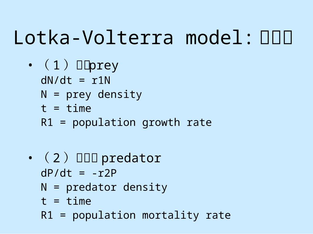
Lotka-Volterra model: 獨立時• ( 1 )獵物 prey
dN/dt = r1NN = prey densityt = timeR1 = population growth rate
• ( 2 )捕食者 predatordP/dt = -r2PN = predator densityt = timeR1 = population mortality rate
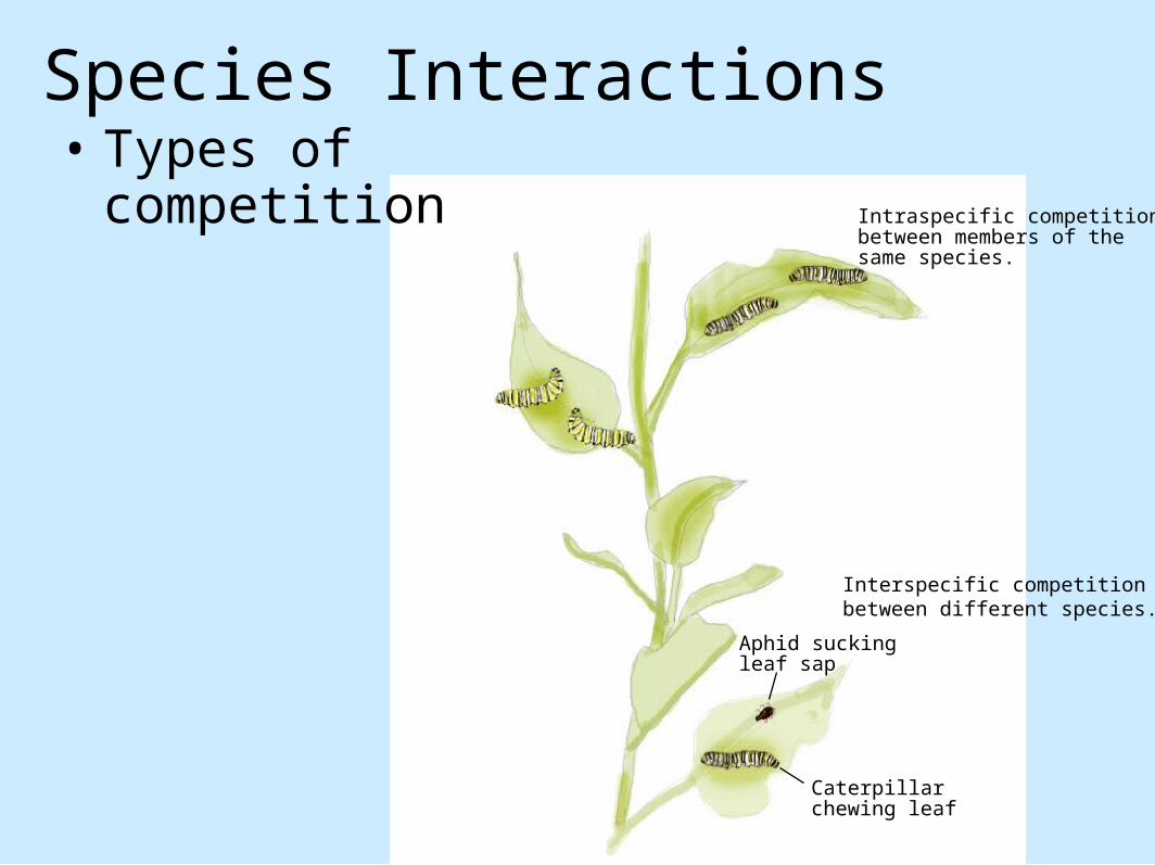
Aphid suckingleaf sap
Caterpillarchewing leaf
Intraspecific competitionbetween members of thesame species.
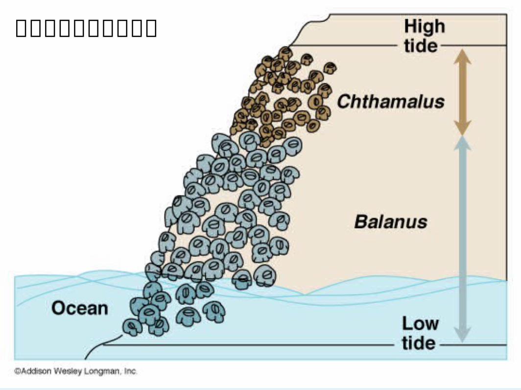
Interspecific competition between different species.
Species Interactions• Types of
competition
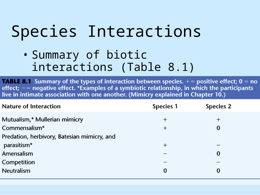
Species Interactions• Summary of biotic interactions (Table 8.1)
Species Interactions• Summary of biotic interactions (cont.)
– Herbivory, predation, parasitism• Positive for one population• Negative for the other population
– Batesian mimicry• Mimicry of a non-palatable species by a palatable
one
Species Interactions– Batesian mimicry (cont.).
• Positive for one population• Negative for the other population
– Amensalism• One-sided competition• One species had a negative effect on another, but
the reverse is not true.
Species Interactions– Neutralism
• Coexistence of noninteracting species• Probably rare
– Mutualism and commensalisms• Less common• Symbiotic relationships
Species Interactions– Mutualism and commensalisms (cont).
• Species are intimately associated with one another• Both species may NOT benefit from relationship• Not harmful, as is the case with parasitism
– Competition• Negative effect for both species
Species Interactions• Types of competition (cont.).
– Interspecific– Intraspecific
• Characterizing competition– Resource competition
• Organisms compete for a limiting resource
Species Interactions• Characterizing competition (cont.).
– Interference competition• Individuals harm one another directly by physical
force
Intraspecific Competition• Quantifying competition in plants vs.
animals– For plants, expressed as change in biomass– For animals, expressed as change in numbers– Plants can not escape competition
Intraspecific Competition• Quantifying competition in plants vs.
animals (cont.).– Animals can move away from competition– Yoda (1963)
• Quantify competition between plants• Yoda's Law or self-thinning rule; 3/2 power rule
Intraspecific Competition– Yoda (1963) (cont.).
• Describes the increase in biomass of individual plants as the number of plant competitors decrease.
• Log w = -3/2 (log N) + log c• w = mean plant weight• N = plant density• C = constant
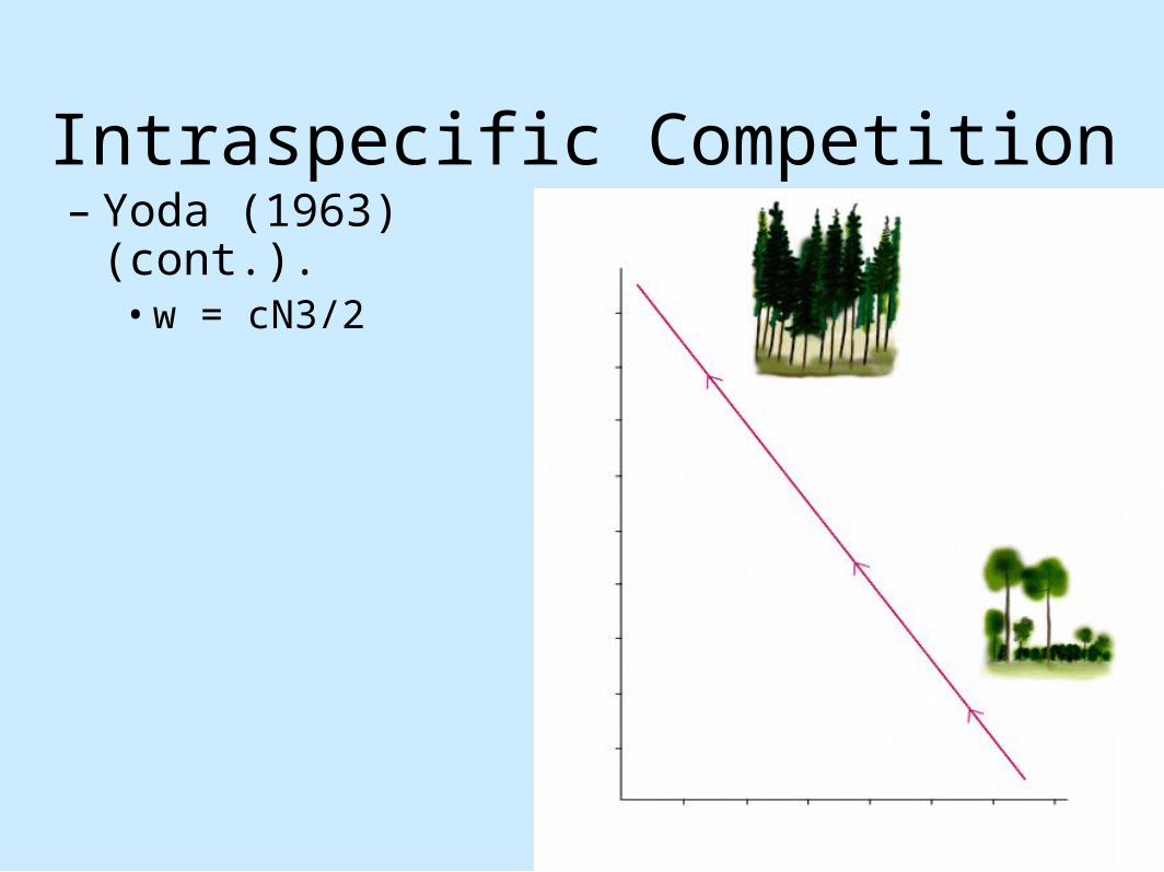
Intraspecific Competition– Yoda (1963) (cont.).
• w = cN3/2
Interspecific Competition: Laboratory Experiments
• Field experiments– Organisms can interact with all other
organisms– Natural variations in the abiotic environment is
factored in
Interspecific Competition: Laboratory Experiments
• Laboratory experiments– All important factors can be controlled– Vary important factors systematically
Interspecific Competition: Laboratory Experiments
• Thomas Park competition experiments– Tribolium castaneum (Figure 8.4a) and
Tribolium confusum
Interspecific Competition: Laboratory Experiments
• Thomas Park competition experiments (cont). – Large colonies of beetles can be grown in
small containers– Large number of replications
Interspecific Competition: Laboratory Experiments
• Thomas Park competition experiments (cont).– Observed changes in population sizes over
two-three years
Interspecific Competition: Laboratory Experiments
• Thomas Park competition experiments (cont). – Waited until one species became extinct
Interspecific Competition: Laboratory Experiments
• Thomas Park competition experiments (cont). – Cultures were infested with a parasite Adelina
Interspecific Competition: Laboratory Experiments
• Thomas Park competition experiments (cont). – T. confusum won 89% of the time Without the
parasite, no clear winner
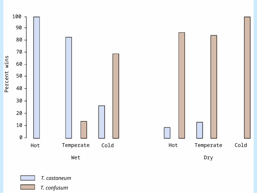
Interspecific Competition: Laboratory Experiments
• Thomas Park competition experiments (cont). – Microclimate effects (Figure 8.4)
10
20
30
40
50
60
70
80
90
100
0
Hot Temperate
Wet
Cold Hot Temperate
Dry
Cold
T. confusum
T. castaneum
Perc
ent
win
s
Interspecific Competition: Laboratory Experiments
– Microclimate effects (cont.).• T. confusum did better in dry environments• T. castaneum did better in moist environments
Interspecific Competition: Laboratory Experiments
• Thomas Park competition experiments (cont).– Mechanism of competition - predation of eggs
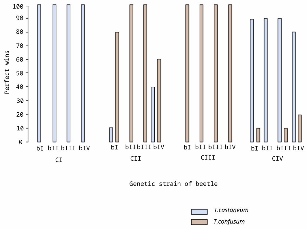
Interspecific Competition: Laboratory Experiments
• Thomas Park competition experiments (cont).– Predatory tendencies varied with different
strains• Figure 8.5
T.castaneum
T.confusum
bI bII bIII bIV bI bII bIII bIV bI bII bIII bIV bI bII bIII bIV0
10
20
30
40
50
60
70
80
90
100Perf
ect
win
s
CI CII CIII CIV
Genetic strain of beetle
Interspecific Competition: Laboratory Experiments
• Interspecific competition: Natural systems– Assessing the importance of competition
• Remove species A and measure the response of species B
Interspecific Competition: Laboratory Experiments
– Assessing the importance of competition (cont.).
• Difficult to do outside of laboratory– Migration problems– Krebs or Cage effect
Interspecific Competition: Laboratory Experiments
– Assessing the importance of competition (cont.).
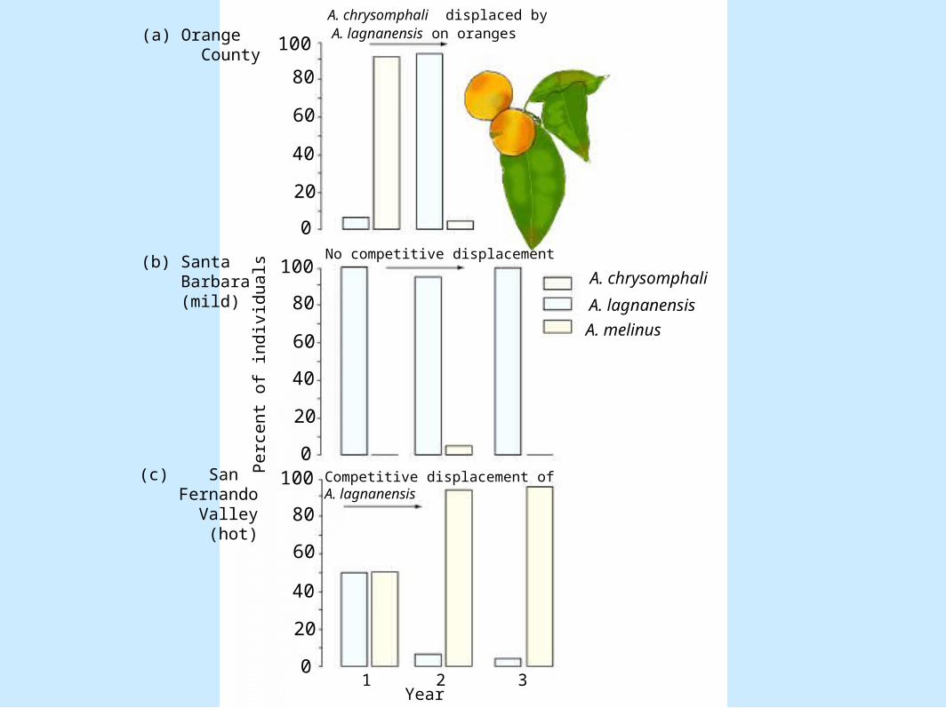
• Examples in nature– Parasitic wasps– Figure 8.6
40
80
60
100
20
0
40
80
60
100
20
0
40
80
60
100
20
0
A. chrysomphali
A. melinus
A. lagnanensis
A. chrysomphali displaced byA. lagnanensis on oranges
No competitive displacement
Competitive displacement ofA. lagnanensis
(a) Orange County
(b) Santa Barbara
(mild)
(c) San Fernando Valley (hot)
1 2 3Year
Perc
en
t of
indiv
iduals
Interspecific Competition: Laboratory Experiments
• Examples in nature (cont.).– Used to control scale pest
– Climate can alter competitive
The Frequency of Competition
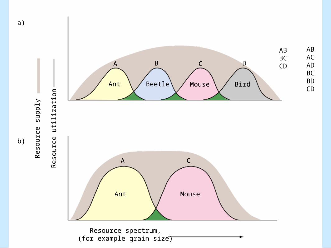
• Joe Connell (1983)– Competition was found in 55% of 215 species
surveyed
– Figure 8.7
ABBCCD
ABACADBCBDCD
A B C D
A C
Ant Beetle Mouse Bird
Ant Mouse
Resource spectrum,(for example grain size)
Reso
urc
e u
tiliz
ati
on
Reso
urc
e s
upply
a)
b)
The Frequency of Competition
• Joe Connell (1983) (cont.).– Effects of number of competing species
• Single pairs: competition was almost always reported (90%)
The Frequency of Competition
– Effects of number of competing species (cont.).• Multiple species, competition was reported in 50%
of the studies
The Frequency of Competition
• Joe Connell (1983) (cont.).– Differing opinions - Schoener (1983)
The Frequency of Competition
• Common flaws of studies– Positive results tend to be more readily
The Frequency of Competition
• Common flaws of studies (cont.).– Scientists do not study systems at random -
may work in systems where competition is more likely to occur
The Frequency of Competition
• Failure to reveal the true importance of competition in evolution and ecological time– Most organisms have evolved to escape
competition and lack of fitness it may confer
The Frequency of Competition
• Failure to reveal the true importance of competition (cont.).– Competition may only occur infrequently and
in years where resources are scarce
The Frequency of Competition
• Patterns of competition– Figure 8.8
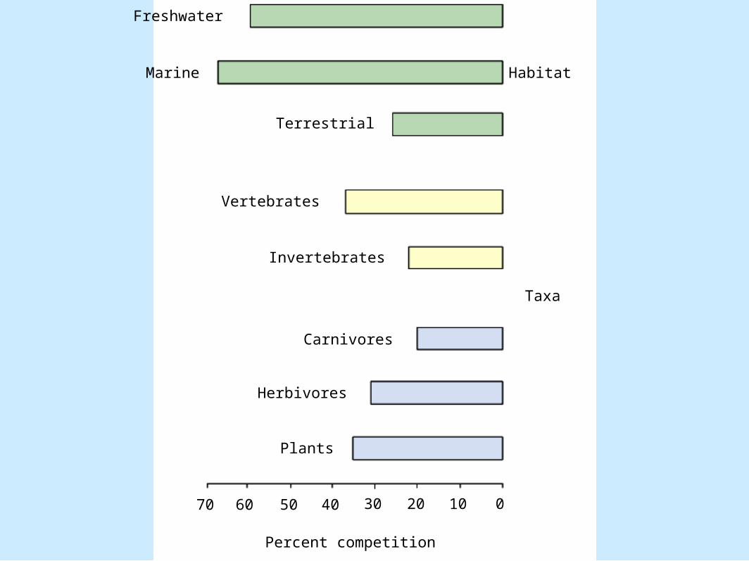
Freshwater
Marine Habitat
Terrestrial
Vertebrates
Invertebrates
Taxa
Carnivores
Herbivores
Plants
70 60 50 40 30 20 10 0
Percent competition
The Frequency of Competition
• Mechanisms of competition (Schoener, 1963)– Table 8.2
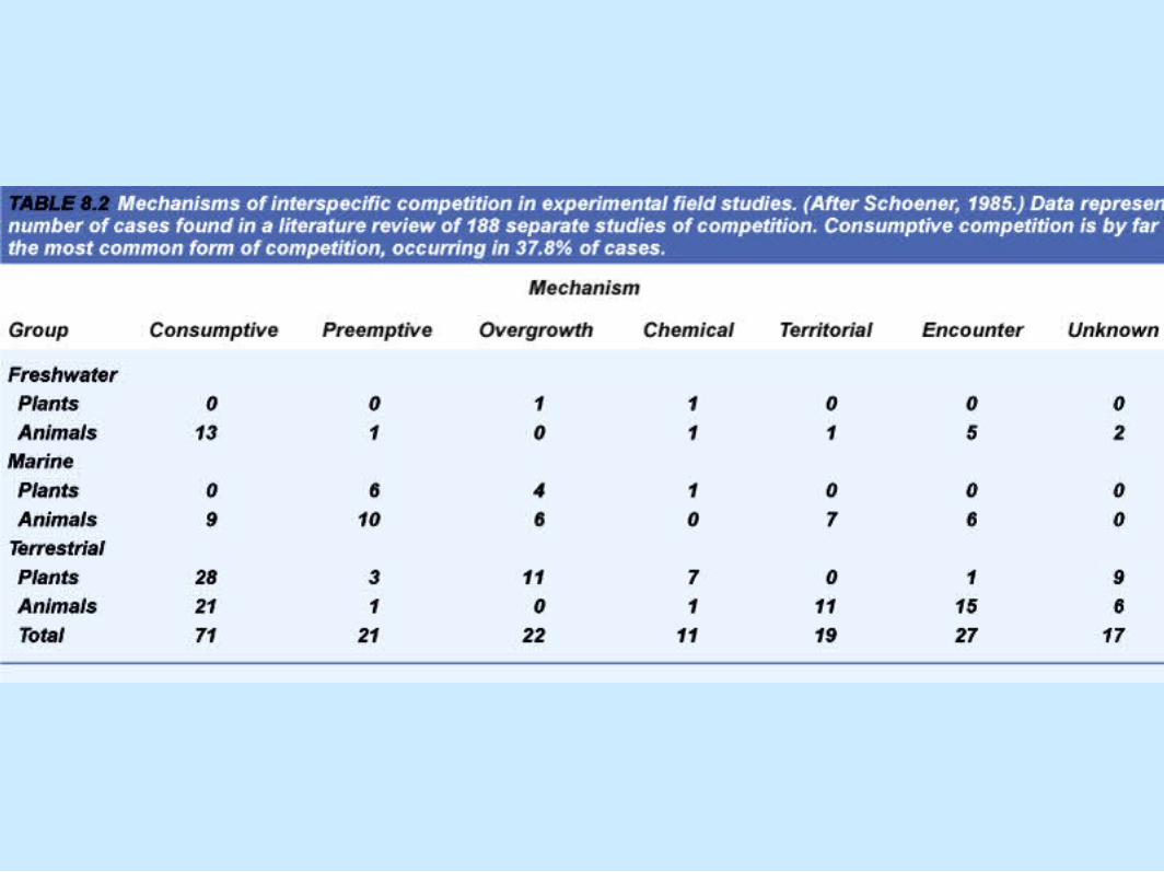
The Frequency of Competition
• Mechanisms of competition (Schoener, 1963) (cont.).– Consumptive or exploitative– Preemtive– Overgrowth
The Frequency of Competition
• Mechanisms of competition (Schoener, 1963) (cont.).– Chemical
• Allelopathy
– Territorial
The Frequency of Competition
• Mechanisms of competition (Schoener, 1963) (cont.).– Encounter
The Frequency of Competition
• Differing views of competition– Gurevitch et al. 1992
• Found no differences in competition between different habitat types but did find filter feeders and herbivores competed more than carnivores or plants.
The Frequency of Competition
• Differing views of competition (cont.).– Grime 1979
• Competition unimportant for plants in unproductive environments
The Frequency of Competition
• Differing views of competition (cont.).– Tilman 1988
• Competition occurs across all productivity gradients
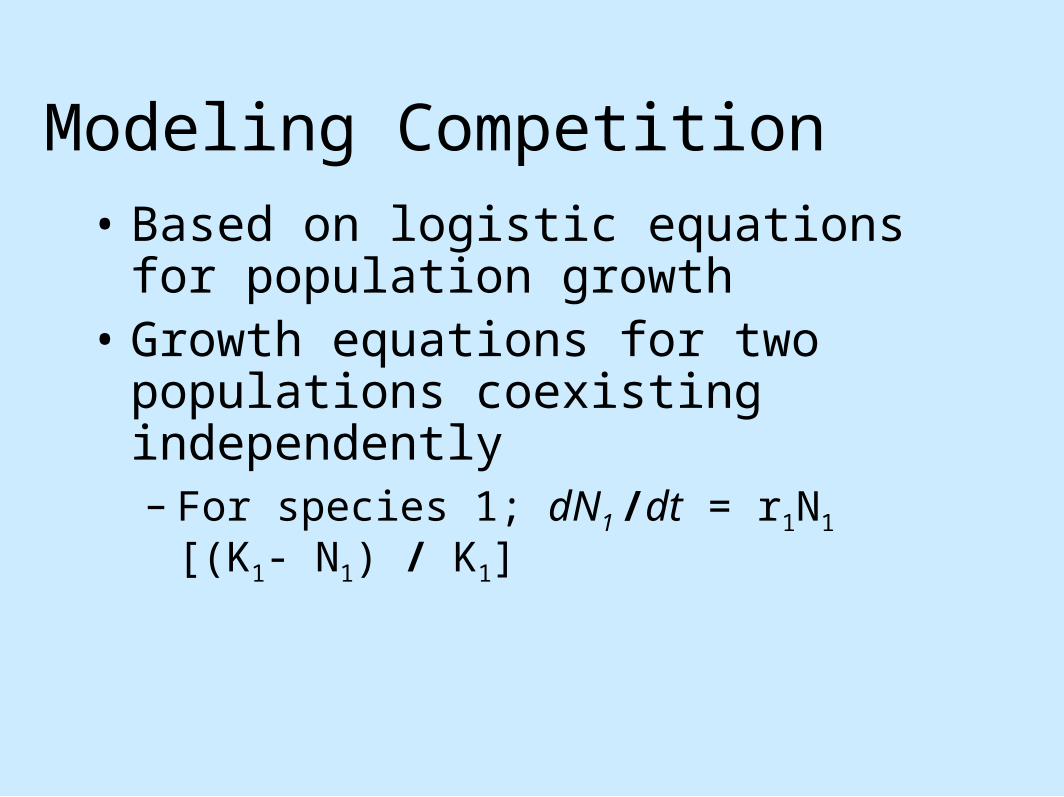
Modeling Competition• Based on logistic equations for population
growth• Growth equations for two populations
coexisting independently– For species 1; dN1 /dt = r1N1 [(K1- N1) / K1]
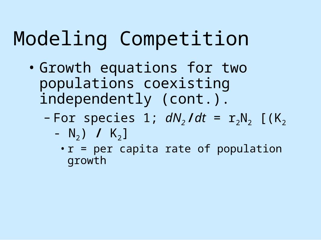
Modeling Competition• Growth equations for two populations
coexisting independently (cont.).– For species 1; dN2 /dt = r2N2 [(K2 - N2) / K2]
• r = per capita rate of population growth
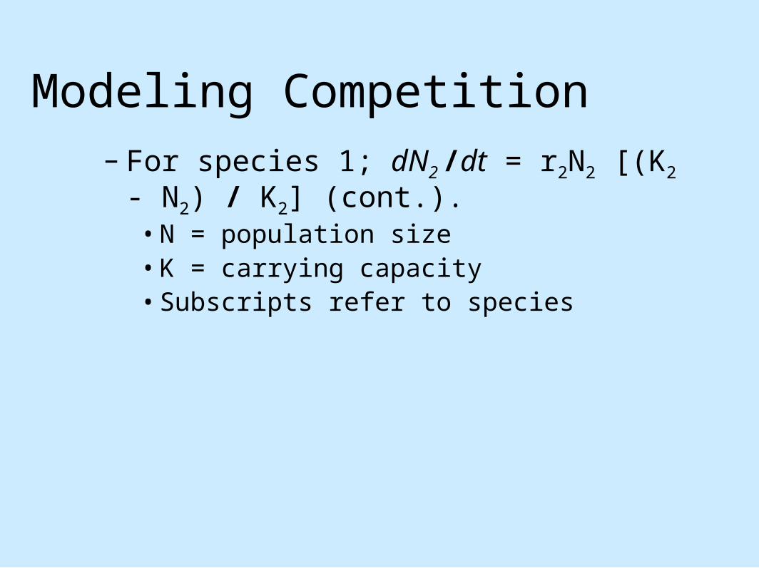
Modeling Competition– For species 1; dN2 /dt = r2N2 [(K2 - N2) / K2]
(cont.).• N = population size• K = carrying capacity• Subscripts refer to species
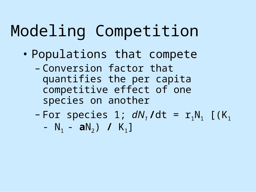
Modeling Competition• Populations that compete
– Conversion factor that quantifies the per capita competitive effect of one species on another
– For species 1; dN1 /dt = r1N1 [(K1 - N1 - aN2) / K1]
Modeling Competition• Populations that compete (cont.).
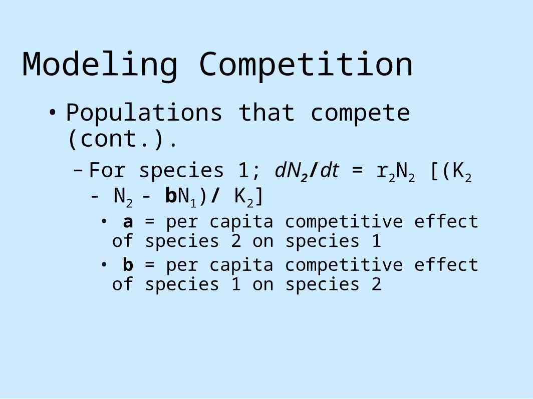
– For species 1; dN2/dt = r2N2 [(K2 - N2 - bN1)/ K2]
• a = per capita competitive effect of species 2 on species 1
• b = per capita competitive effect of species 1 on species 2
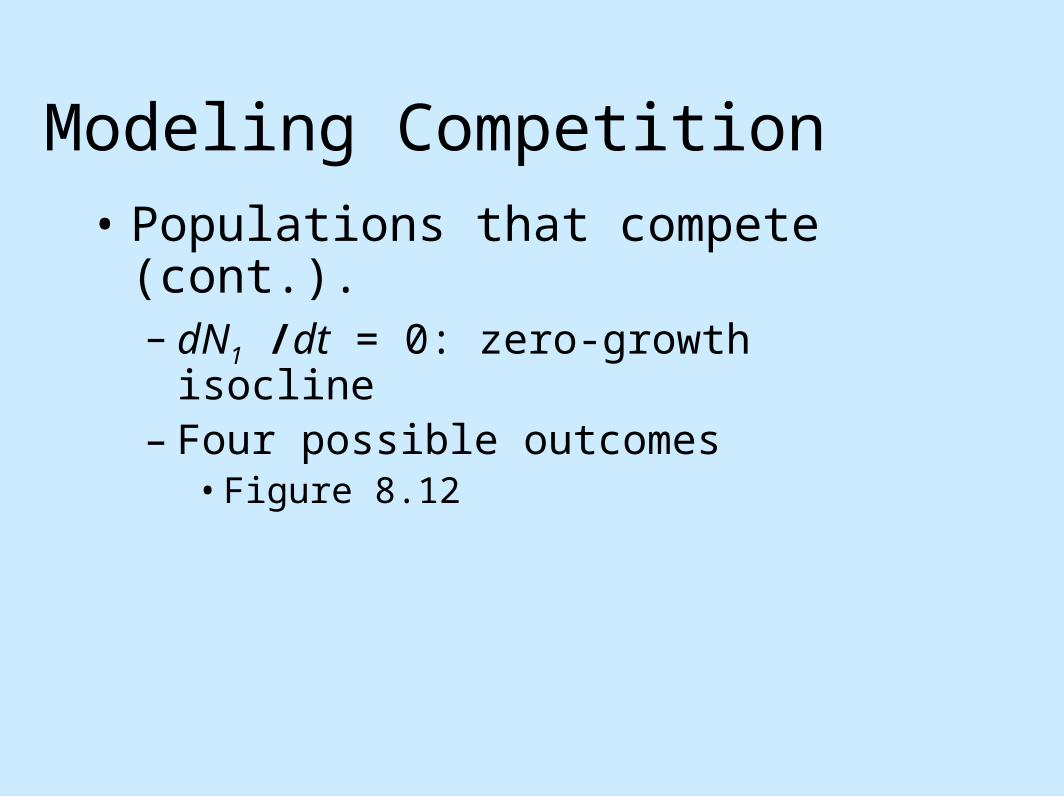
Modeling Competition• Populations that compete (cont.).
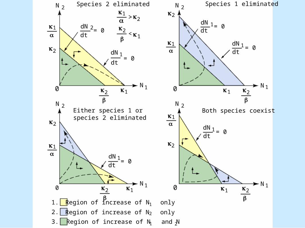
– dN1 /dt = 0: zero-growth isocline– Four possible outcomes
• Figure 8.12
N
NN
2 N 2
N
NN
N2 2
Region of increase of N only1
Region of increase of N only2
2Region of increase of N and N1
1.
2.
3.
Species 2 eliminated Species 1 eliminated
Either species 1 or species 2 eliminated
Both species coexist
2
2
2
2
1
1
1
1
1
00
0 0
1
1
1
2
2 2
21 1
11
1
dNdt
2
1dNdt
= 0
= 0
1dNdt
= 0
1dNdt
= 0
1dNdt
= 01dN
dt= 0
2
>
<
2
1
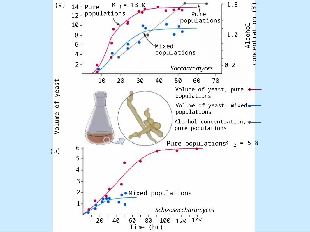
Modeling Competition• Test of equations
– Figure 8.13
2
4
6
8
10
1214
0.2
1.0
1.8
Alc
ohol
conce
ntr
ati
on (
%)
10 20 30 40 50 60 70
Pure populations
K = 13.0
Mixed populations
Pure populations
(a)
Volume of yeast, purepopulations
Volume of yeast, mixed populations
Alcohol concentration, pure populations
1
2
3
4
5
6
20 40 60 80 100 120 140
Pure populations K = 5.82
Mixed populations
Schizosaccharomyces
Time (hr)
Saccharomyces
(b)
Volu
me o
f yeast
1
Modeling Competition• Deficiencies
– The maximal rate of increase, the competition coefficients, and the carrying capacity are all assumed to be constant
– There are no time lags
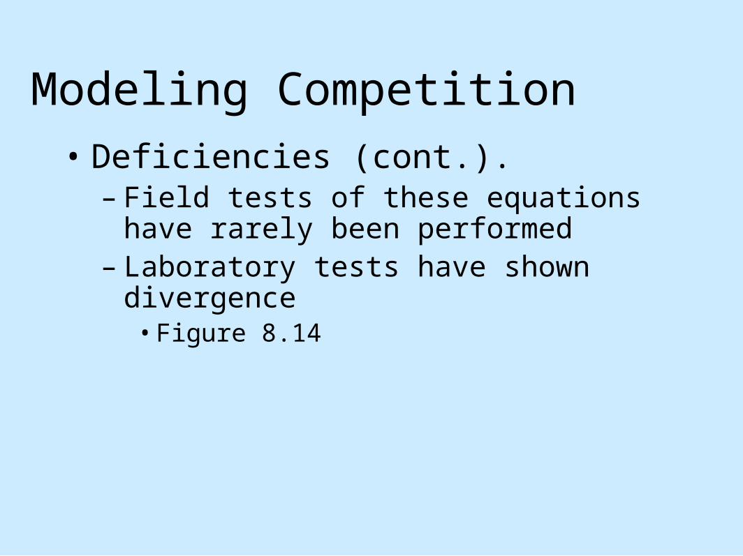
Modeling Competition• Deficiencies (cont.).
– Field tests of these equations have rarely been performed
– Laboratory tests have shown divergence• Figure 8.14
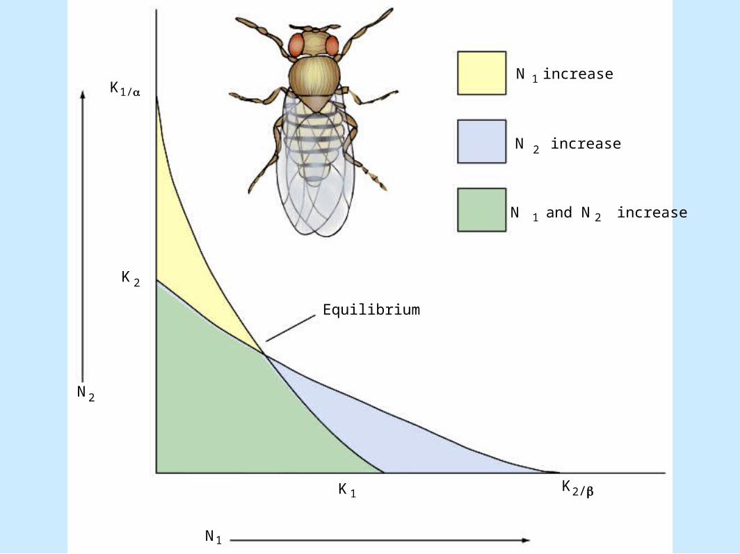
N increase
N increase
N and N increase
1
2
1 2
Equilibrium
K1
1N
N2
K 2
K1/
2/K
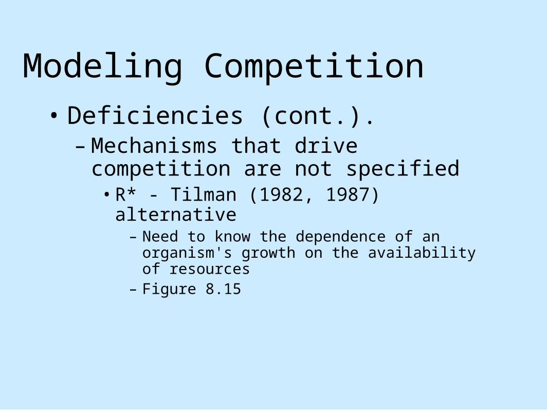
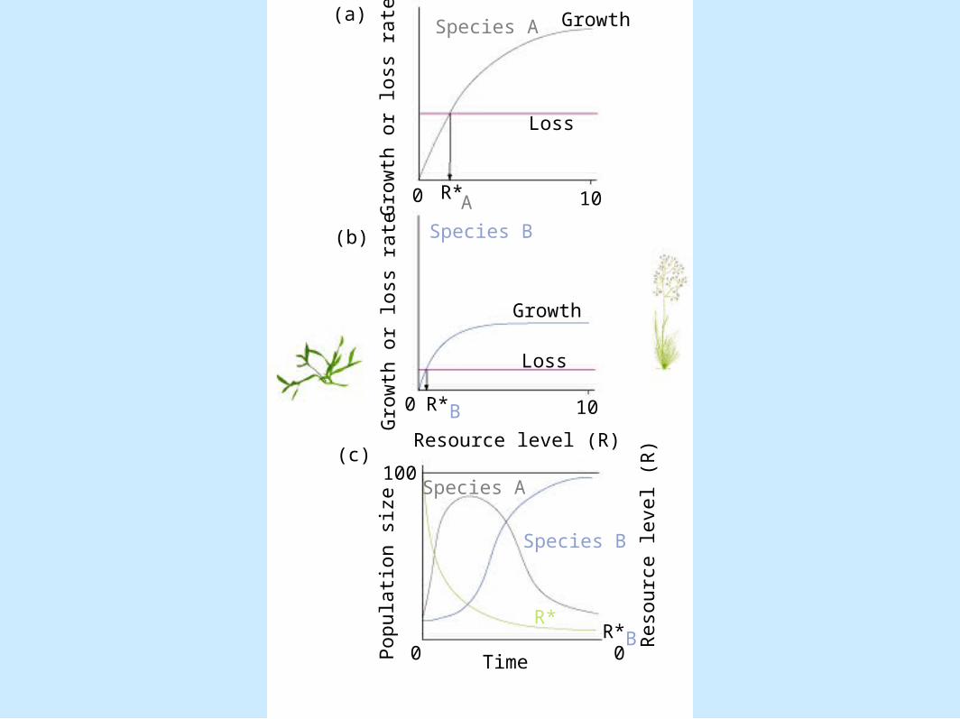
Modeling Competition• Deficiencies (cont.).
– Mechanisms that drive competition are not specified
• R* - Tilman (1982, 1987) alternative– Need to know the dependence of an organism's growth on
the availability of resources– Figure 8.15
Gro
wth
or
loss
rate
Gro
wth
or
loss
rate
Popula
tion s
ize
(a)
(b)
(c)100
Species A
Species B
Species A
Species B
Loss
100 R*A
0 R*B
Loss
Growth
Resource level (R)
Time0 0
Growth
10
R*BR* R
eso
urc
e level (R
)
Coexistence of Species• Niche
– Grinnell (1918): a subdivision of a habitat that contains an organism's' dietary needs, its temperature, moisture, pH, and other requirements
Coexistence of Species• Niche (cont.).
– Elton (1927) and Hutchinson (1958): an organism's role within the community
• Gause: two species with similar requirements could not live together in the same place
Coexistence of Species• Hardin (1960): Gause's principle, known
as competitive exclusion principle, where direct competitors cannot coexist
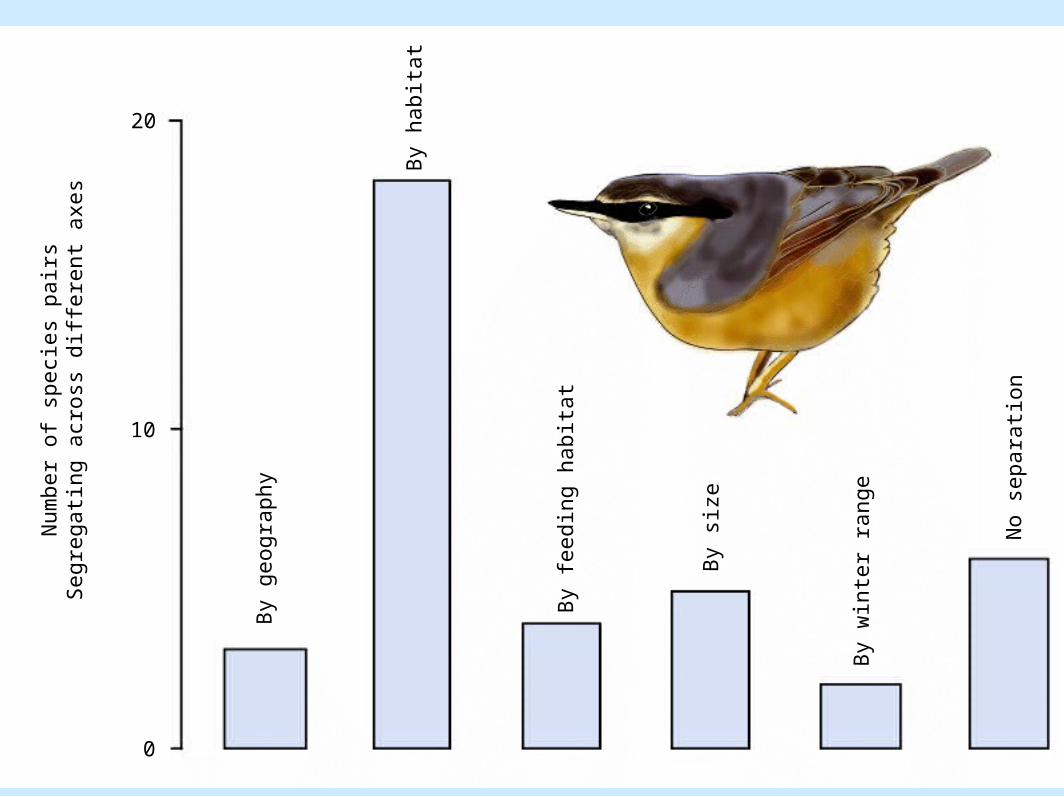
Coexistence of Species• David Lack: Competition and coexistence
in about 40 pairs of birds, mediated by habitat segregation.– Figure 8.16
By h
abit
at
0
10
20
Num
ber
of
speci
es
pair
sSegre
gati
ng a
cross
diff
ere
nt
axes
By g
eogra
phy
By f
eedin
g h
abit
at
By s
ize
By w
i nt e
r ra
nge
No s
epara
tion
Coexistence of Species• Examples of coexistence
– Darwin's finches on the Galaapagos– Terns on Christmas Island (Ashmole 1968)
Coexistence of Species• Ranks for resource partitioning (Schoener
1974)– Macrohabitat (55%)– Food type (40%)– Time of day or year (5%)
Coexistence of Species• Hutchinson (1959)
– Seminal paper, "Homage to Santa Rosalia, or why are there so many kinds of animals?"
– Examined size differences for• Sympatric species (species occurring together)

Coexistence of Species• Hutchinson (1959) (cont.).
– Examined size differences for (cont.).• Allopatric species (occurring alone)• Table 8.3
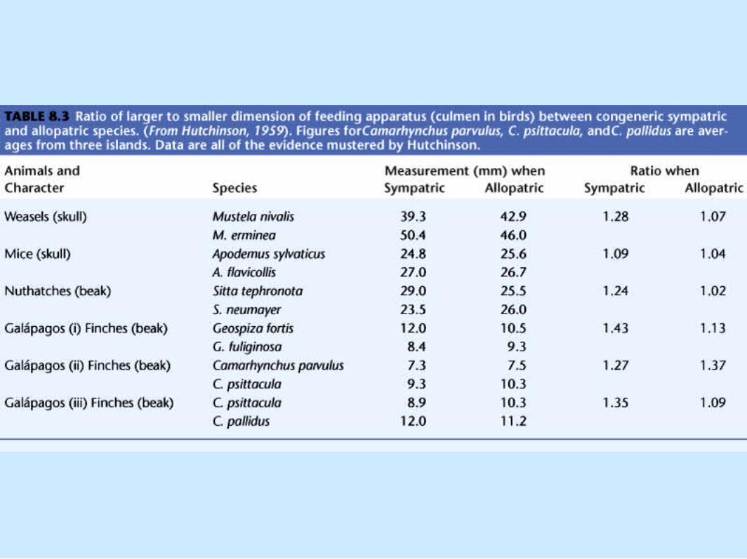
Coexistence of Species– Examined size differences for (cont.).
• Hutchinson's ratio, 1.3
– Criticism of Hutchinson• Studies that supported Hutchinson - inappropriate
statistics
Coexistence of Species– Criticism of Hutchinson (cont.).
• Further tests showed no differences between species than would occur by chance alone.
• Size-ratio differences could have evolved for other reasons
Coexistence of Species– Criticism of Hutchinson (cont.).
• Biological significance cannot always be attached to ratios, particularly to structures not used to gather food. Figure 8.17

Coexistence of Species• Hutchinson (1959) (cont.).
– Support of Hutchinson– Figure 8.18 d/w analysis for separation on
continuous resource sets

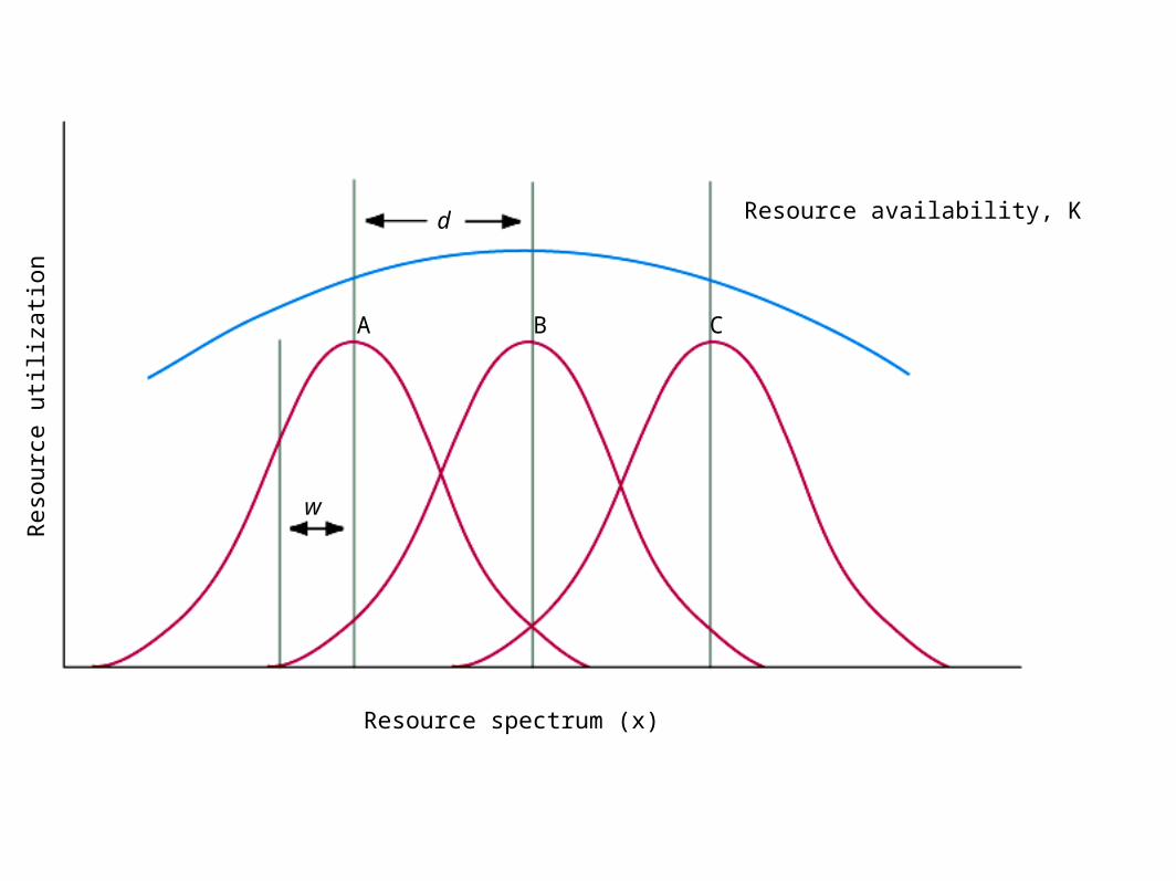
Coexistence of Species– Figure 8.18 d/w analysis for separation on
continuous resource sets (cont.).• Figure 8.19
Reso
urc
e u
tiliz
ati
on
Resource availability, K
Resource spectrum (x)
d
A B C
w
Coexistence of Species• Figure 8.19 (cont.).
– d=distance between maxima– w = measure of spread
• Figure 8.20
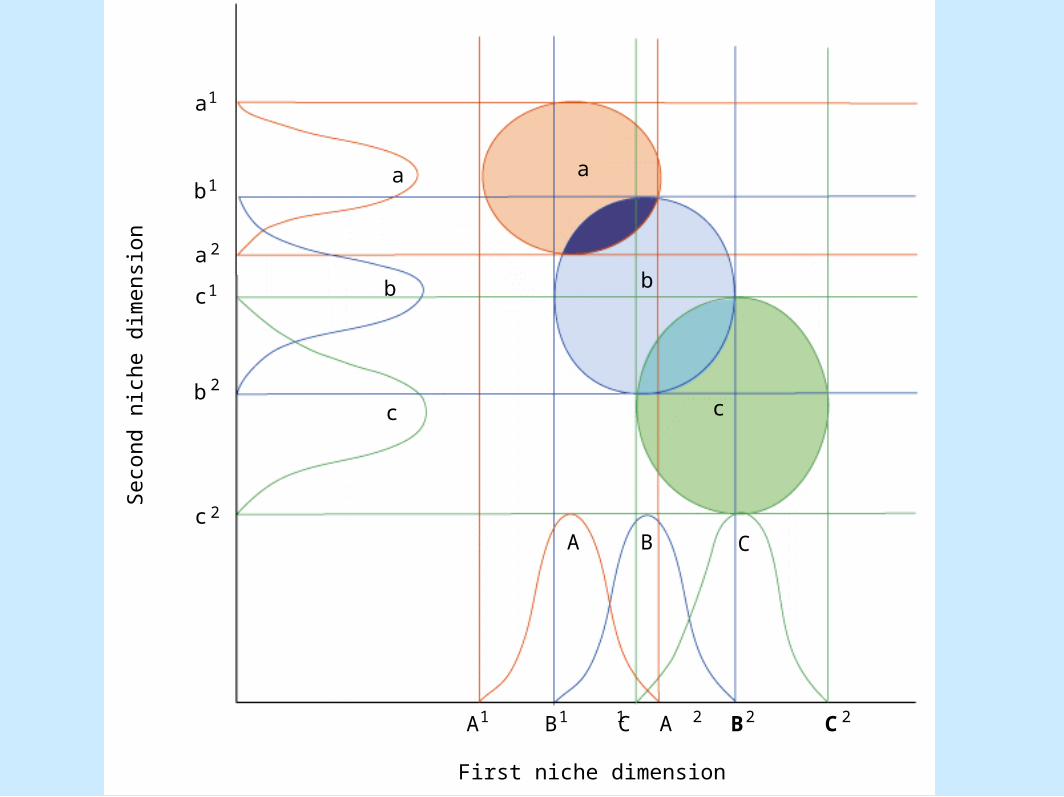
a
b
a
c
b
c
1
1
2
1
2
2
a
b
c
a
b
c
A B C
B C B C1 1 1 2 2 2A
First niche dimension
Seco
nd n
iche d
imensi
on
A
Coexistence of Species• Hutchinson (1959) (cont.).
– Discontinuous resource distribution• Figure 8.21
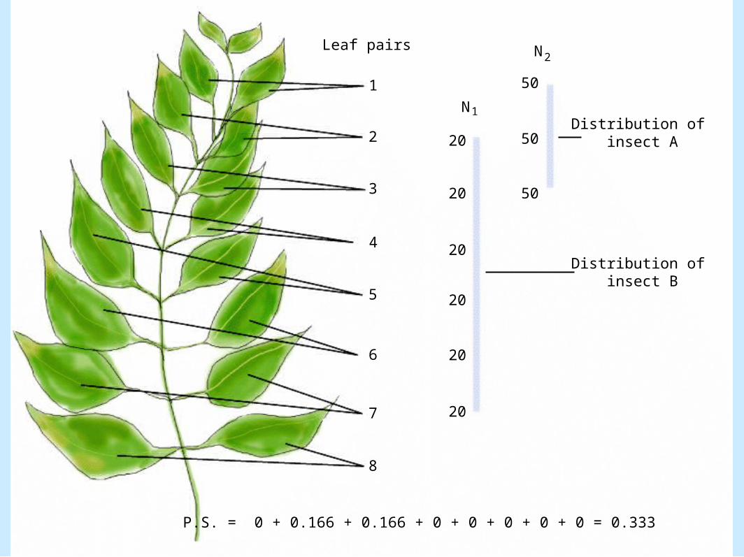
1
2
3
4
5
6
7
8
20
20
20
20
20
20
50
50
50
Leaf pairs N2
Distribution of insect A
Distribution of insect B
P.S. = 0 + 0.166 + 0.166 + 0 + 0 + 0 + 0 + 0 = 0.333
N1
Coexistence of Species– Discontinuous resource distribution (cont.).
• Figure 8.22
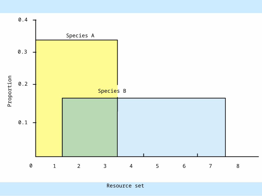
Species A
Species B
0.4
0.3
0.2
0.1
0 4 5 6 72 31 8
Resource set
Pro
port
ion
Coexistence of Species– Discontinuous resource distribution (cont.).
• Niche overlap between two insect species that feed on a shrub
– Measured quantity» PS = Spi
» PS = proportional similarity» S = sum of all units, 1 to n, in resource set
Coexistence of Species– Measured quantity (cont.).
» pi = proportion of least abundant member of pair» PS < 0.70 indicates coexistence for single resource» PS > 0.70 indicates competitive exclusion for single
resource
Coexistence of Species– Measured quantity (cont.).
» Proportional similarity indices for two or more resources can be combined
•Multiply separate PS values to determine overall PS value•Coexistence for two resources
– 0.7 x 0.7 = 0.49 or less
Applied Ecology• Is the release of multiple species of
biological control agents beneficial?– Control of pests in agriculture is of paramount
importance
Applied Ecology• Is the release of multiple species of
biological control agents beneficial? (cont.).– Biological control is seen as a preferable
alternative to chemical control
Applied Ecology– Biological control viewed by some
• Release a variety of enemies against a pest• Observe which enemy does the best job
Applied Ecology– Biological control viewed by some (cont.).
• Is this the best strategy?– Intensive competition for the prey leads to lower
effectiveness of the biological agents– Greater population establishment rate with fewer enemy
species (Figure 1 for Box 1)

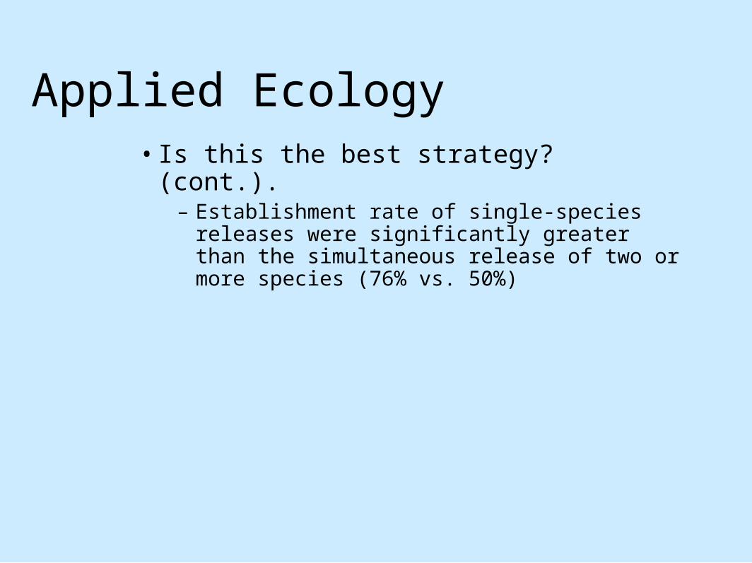
Applied Ecology• Is this the best strategy? (cont.).
– Establishment rate of single-species releases were significantly greater than the simultaneous release of two or more species (76% vs. 50%)
Summary• Competition may be interspecific or
intraspecific• Competition may be viewed as resource
competition or interference competition
Summary• Intraspecific competition between plants
may be described by the 3/2 self-thinning rule
Summary• Outcome of competition can be influenced
by– Environmental conditions– The presence or absence of natural enemies
Summary• Outcome of competition can be influenced
by (cont.).– The genetic strain of the competitors involved
Summary• Experimental studies show that in nature
competition occurs between different types of organisms over a broad scale– Such studies focused on exotics and
generalizations to natural ecosystems are questionable
Summary• Experimental studies show that in nature
competition occurs (cont.).– Competition between exotics and native
species• Serious consequences for natural ecosystems
Summary• Frequency of competition
– 55% to 75% of species involved– Competition is often asymmetric
• Six mechanisms of competition– Consumptive– Preemptive
Summary• Six mechanisms of competition (cont.).
– Overgrowth– Chemical– Territorial– Encounter
Summary• Lotka-Volterra model: early competition
model– Two species interaction– Four possible outcomes
• Species 1 becomes extinct• Species 2 becomes extinct
Summary– Four possible outcomes (cont.).
• Either species 1 or species 2 becomes extinct based on starting conditions
• Coexistence
Summary• Lotka-Volterra model: early competition
model (cont.).– Competition is minimized and species can
coexist if they use different resources• Hutchinson's 1:1.3 ratio
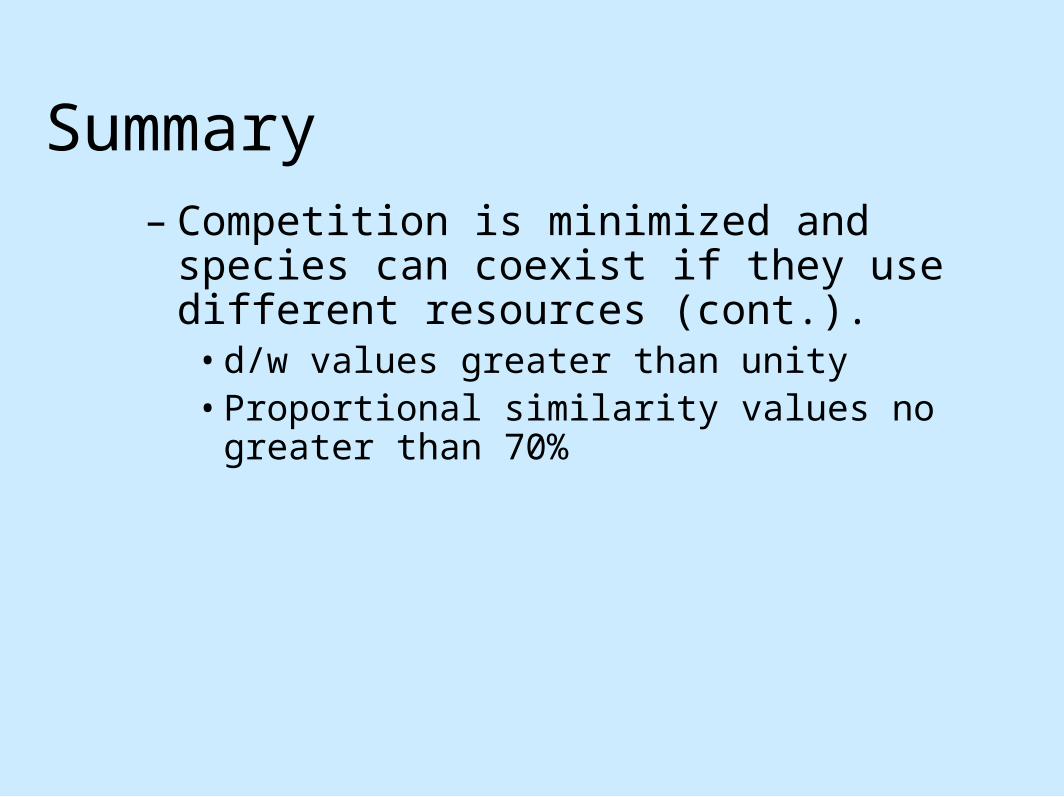
Summary– Competition is minimized and species can
coexist if they use different resources (cont.).• d/w values greater than unity• Proportional similarity values no greater than 70%
Discussion Question #1• Which type of competition would you
expect to be more important in nature?
Discussion Question #2• Much native vegetation in the Florida
Everglades is being lost. Could this be due to climate change or the influence of exotic invaders? Design an experiment.
Discussion Question #3• In the above question, how could you
determine the mechanism of competition? How could you differentiate among competition for light, water, or nutrients?
Discussion Question #4• In trying to understand how species
compete, what advantages are there in field observations, field experiments, laboratory experiments, and mathematical models?
Discussion Question #5• Using fully labeled graphs, explain the Lotka-
Volterra approach to competition theory. What predictive power does the Lotka-Volterra model have? How is Tilman's R* concept an improvement? What other improvements might you suggest?