1  

ComparisonoftheWRFandHIRHAMmodelsoverSvalbard

SVALIDeliverableD3.1‐4

Report 

MARIA NORMAN1, BJÖRN CLAREMAR

1 

RUTH MOTTRAM2, ANNA RUTGERSSON1 

 

1DEPARTMENT OF EARTH SCIENCES, UPPSALA UNIVERSITY 

2DANISH METEOROLOGICAL INSTITUTE 

JULY 2014 

 

 

2  

AbstractThe glacier mass balance is influenced by meteorological conditions. Atmospheric models provide 

high spatial and temporal coverage of meteorological data, which is especially important in an area 

of sparse measurements, such as the Arctic. When simulating the Arctic, it is important to use model 

physics schemes and a resolution which capture the specific conditions in the Arctic area. 

Meteorological parameters over Svalbard from two regional models, WRF and HIRHAM (5.5 km 

resolution), are analyzed and compared in the present study. The results are validated against 

measurements from Automatic Weather Stations at three glaciers. Meteorological parameters, such 

as air temperature, specific humidity, wind speed and direction, are studied. The models agree quite 

well with each other, and with observations. Air temperature is the parameter with best model‐

measurement correlation, although the temperature is slightly lower than observed in both models. 

The specific humidity is overestimated by WRF, and underestimated by HIRHAM. The wind speed is 

difficult to simulate, and the agreement with observations strongly depend on the wind direction. 

Evaluating the two atmospheric models at three glaciers during a limited time period, WRF is slightly 

closer in magnitude to the observed values than HIRHAM.   

3  

1.IntroductionOver the last century, the Svalbard archipelago has experienced a significant thinning of the glacial 

mass which is most likely an effect of the global warming (Vaughan et al., 2013). To better 

understand the processes affecting the preceding and present changes, and to simulate future 

changes, it is important to have knowledge of the glacier‐atmosphere interaction. The mass balance 

of a glacier is the difference between accumulation and ablation (sublimation and melting), which 

are highly influenced by atmospheric processes. The estimation of the mass budget in a glacier model 

therefore requires meteorological input such as temperature, humidity, wind, precipitation, 

turbulent heat fluxes, and radiation. Due to sparse atmospheric measurements in the Arctic, 

modelling is an important tool to obtain a good spatial and temporal coverage of meteorological 

parameters. Model simulation in an area such as Svalbard is challenging due to the variable 

topography causing local weather phenomena, lack of knowledge of atmospheric processes during 

long polar nights/midnight sun, and the seasonal variability of land‐ and sea ice affecting turbulent 

fluxes of heat and water vapor. The performance of the model is therefore highly dependent on the 

horizontal resolution and the physics scheme (Claremar et al, 2012). 

The aim of this study is to evaluate two atmospheric models, WRF and HIRHAM, by comparing 

meteorological near‐surface parameters with measurements. The parameters investigated are air 

temperature, specific humidity, and wind speed. Differences in spatial patterns over the Svalbard 

area, as well as case studies at three key places are analysed. 

2.Modelsandmeasurements

2.1WRFModelThe Weather Research and Forecasting (WRF) model (Skamarock et al., 2008) is a numerical weather 

prediction (NWP) and atmospheric simulation system which can be used both for research and 

operational applications. WRF is a flexible, state‐of‐the‐art, portable code with a variety of physical 

and dynamical options. The model can be applied for a broad range of scales from large‐eddy to 

global simulations. The model domain has a horizontal resolution of 16.5 km, which is nested to a 

domain resolution of 5.5 km. The resolution used in this study is 5.5 km and the model setup is the 

same as in Claremar (2013), where the WRF3.5 version is used. The forcing data is from the ERA‐

Interim re‐analysis (Dee et al., 2011). The model domain for the 5.5 km resolution is shown in Figure 

1a. 

2.2HIRHAMModelThe HIRHAM model (Christensen et al., 1996; Christensen et al., 2007) is an atmospheric climate 

model which combines the dynamics of HIRLAM (Undén et al, 2002) with the physical 

parameterizations schemes from ECHAM (Roeckner et al., 2003). HIRLAM is a numerical short‐range 

weather forecasting model, used for routine forecasting, and ECHAM global climate model is a 

general atmospheric circulation model developed by the Max Planck Meteorological Institute (MPI). 

The original HIRHAM model was developed in collaboration with DMI (the Danish Meteorological 

Institute) and MPI. The version of HIRHAM used in the present study is HIRHAM version 5, based on 

HIRLAM 7.0 and ECHAM 5.2.02. In this study, the model horizontal resolution is 5.5 km, and the 

forcing data is from the ERA‐Interim re‐analysis. HIRHAM is not nested, and the model domain for 5.5 

km resolution is larger than the WRF domain (Figure 1b). 

4  

     

Figure 1 Model domain for WRF (a) and HIRHAM (b) with 5.5 km resolution. The contour lines show terrain with 200 m equidistance up to 1200 m (a large area of the terrain on Greenland exceeds 1200 m). 

2.3MeasurementsThe two models are verified using observations from three Automatic Weather Stations (AWS) 

located at glaciers on Svalbard. The three stations are: Nordenskiöldbreen (78°41’39’’N, 17°09’22’’E, 

530 m a.s.l.), Kongsvegen (78°46’49’’N, 13°09’22’’E, 537 m a.s.l.),  and Vestfonna (79°56’03’’N, 

19°11’08’’E, 305 m a.s.l.). For the locations of the stations see Figure 2, and for details about the 

instrumentation see Table 1. 

 

Figure 2 Map of Svalbard and location of the AWS: Nordenskiöldbreen (A), Kongsvegen (B), and Vestfonna (C) (from Norwegian Polar Institute, http://toposvalbard.npolar.no/?lang=en). 

Nordenskiöldbreen is a glacier of 193 km2 (5 km wide and 17 km long), and the AWS is located in the 

central flow confined by steep slopes to the north and south. The slope of the glacier at the position 

of the AWS is southwest, and the direct surroundings are relatively smooth and homogeneous. 

Further details about Nordenskiöldbreen AWS and the topography are given by den Ouden et al. 

(2010), Van Pelt et al. (2011), and on http:/www.projects.science.uu.nl/iceclimate/aws/. Kongsvegen 

glacier has an area of 102 km2 (length 26 km) with a northwesterly slope. The surface at the AWS is 

A B 

C 

a)  b) 

5  

virtually smooth and homogenous, and further information about the site can be found in Obleitner 

and Lehning (2004). Vestfonna, which cover 2400 km2 of the western part of Nordaustlandet, is the 

second largest ice cap on Svalbard. The AWS is located on the western slope of the ice cap, and the 

direct vicinity is smooth and homogenous. Further details of the site are given in Möller et al. (2011) 

and Pohjola et al. (2011). 

Table 1 Details and instrumentation at the AWS sites. Showing the period of available data, height above sea level (a.s.l.), and the instrumentation for temperature, humidity, and wind measurements. 

AWS  Period  Height  Temp/hum  Wind 

Nordenskiöldbreen  March 2009 – March 2010  530 m a.s.l.  Vaisala HMP45A 

Young Wind Monitor RM 05103 

Kongsvegen  April 2008 – April 2010  537 m a.s.l.  Rotronic Hygroclip 

Young Wind Monitor RM 05103 

Vestfonna  April 2008 – April 2009  305 m a.s.l.  Vaisala HMP45A 

Young Wind Monitor RM 05103 

At all three sites wind speed and direction were measured with Young Wind Monitor RM 05103. 

Temperature and humidity were measured using a Vaisala probe at Nordenskiöldbreen and 

Vestfonna, while a Rotronic devise were used at Kongsvegen. The humidity sensors were calibrated 

to measure relative humidity with respect to water. Based on the ratio of saturated vapor pressure, 

the humidity data were converted to represent relative humidity with respect to ice. Temperature, 

humidity, and wind are measured at 4.5 m height above the surface at Nordenskiöldbreen during the 

period March 2009 to March 2010. At Kongsvegen temperature and humidity are measured at 3.5 m 

above the surface, while wind is measured at 4.5 m. The Kongsvegen measurements are from the 

time period April 2008 to April 2010. Temperature and humidity at Vestfonna are measured at 1.8 m 

height above surface, while the wind is measured at 2 m. The measurement period on Vestfonna is 

April 2008 to April 2009. 

3.Methodology

3.1TemperaturecorrectionWhen comparing model results with observations, a model grid point close to the AWS station where 

the model height above sea level agrees best with the station height above sea level, is chosen. The 

chosen grid point might nonetheless deviate in height compared to the AWS, and since the air 

temperature in most areas decreases with height, this could result in a model temperature not 

representative for the AWS.  To correct for the difference in height, the slantwise temperature 

profile is calculated by linear interpolation using the AWS grid point together with the surrounding 

eight grid points (Figure 3). The temperature at the AWS height above sea level is then used in the 

analyses.  

This correction is made for the three selected sites each time step, and for the two models 

separately. Others, e.g. Sterns et al. (1997), Pohjola et al. (2002), and Hines and Bromwich (2008) 

used constant lapse rates of ‐0.0071 °C m‐1 and ‐0.0044 °C m‐1. A constant lapse rate does not include 

changes in atmospheric conditions such as occasions when the temperature increase with height. 

Our approach has the advantage that the lapse rate changes with the atmospheric conditions. It is 

found that the lapse rates for the sites in this study varies between ‐0.0242 °C m‐1 and +0.0158 °C m‐1 

using WRF, and between ‐0.0301 °C m‐1 and +0.0214 °C m‐1 using HIRHAM. The average lapse rates 

are ‐0.0060 °C m‐1 and ‐0.0046°C m‐1 using WRF and HIRHAM, respectively. Since the maximum 

6  

height differences are 113 m (WRF) and 94 m (HIRHAM), the maximum temperature corrections 

during negative lapse rate are 2.9°C and 3.2°C, respectively. During positive lapse rate, the maximum 

temperature corrections are 1.3 °C and 1.7 °C, respectively. The number of cases with positive lapse 

rates varies at the three sites and with the model used. At Nordenskiöldbreen 5% and 9% of the 

cases have positive lapse rates for WRF and HIRHAM, respectively. The corresponding numbers at 

Kongsvegen are 3% and 24%; while at Vestfonna 5% and 12% are cases with positive lapse rates 

using WRF and HIRHAM, respectively.  

From the slantwise temperature profiles, assuming that a lapse rate larger than ‐0.01 represent 

stable atmospheric conditions, it can be concluded that the stable conditions dominate the 

atmosphere over Svalbard. In WRF, 94%, 80%, and 94% of the days show stable conditions at 

Nordenskiöldbreen, Kongsvegen, and Vestfonna, respectively. The corresponding amounts of stable 

cases in HIRHAM are 82%, 95%, and 91%. 

 

Figure 3 Temperature profiles with the temperature vs. height above sea level calculated using the grid point at the AWS station Vestfonna (blue dot with red circle), and four surrounding grid points (blue dots) using WRF (a) and HIRHAM (b). The straight line is a linear interpolation between the dots. The temperature at the AWS height (dashed line) is used in the analysis in the present study. 

3.2WindcorrectionThe wind at the AWS’s are measured below 10 m height, and the 10m wind will therefore 

presumable be underestimated. In Claremar et al. (2012) the measured AWS wind were corrected 

using Monin‐Obukhov theory. The wind speed was approximated to increase by 15% at 

Nordenskiöldbreen, 20% at Kongsvegen, and 25% at Kongsvegen in order to represent the 10 m 

wind. This correction of the AWS wind is also applied in the present study. 

7  

3.3TaylordiagramTaylor (2001) developed a method where different type of statistics can be illustrated in a single 

figure. In a Taylor diagram the standard deviation, the correlation coefficient, and the root mean 

square difference (RMSD) is presented. With this type of diagram the similarity between 

observations and one or several models is presented.  

The correlation coefficient, R, is defined as: 

 ∑ ̅ ̅

,  (1)  

where fn and rn are two variables defined at N discrete points. For practice use when comparing 

model and measurements, f represent measurement, and r represent model data. R is the 

correlation coefficient between f and r.   ̅and  ̅  are mean values, and σf and σr are standard 

deviations of f and r, respectively. The RMSD is defined as: 

  ∑/.  (2) 

To separate the difference in patterns from the difference in mean between f and r, RMSD can be 

divided into two components. The overall bias is defined as   ̅ ̅ ,and the centered pattern RMSD is defined as: 

  ′ ∑ ̅ ̅/.  (3) 

The full RMSD is yielded by adding the two components quadratically: 

  ′   (4) 

One diagram with the above statistical quantities can be constructed using the relationship: 

  2 ,  (5)  

together with the law of cosines: 

  2 ∙ ,  (6) 

where a, b and c are length of sides in a triangle, and   is the angel opposite to side c. The geometric 

relationship between RMSD’, R, σf, and σr is shown in Figure 4. 

 

 

 

 

 

RMSD’ σf

σr

cos‐1 R 

Figure 4 The geometric relationship between the centered pattern RMSD’, the correlation coefficient R, and the standard deviation σf and σr of observation and model. 

8  

4.ResultsIn this section a comparison between the variables air temperature, specific humidity, and wind 

using WRF and HIRHAM is presented. Spatial patterns as well as statistics at three key places are 

analyzed.  Taylor diagrams are used to compare the model results, and to validate with 

measurements. For the spatial comparison between the two models, the period 2008‐2011 is used, 

while for the comparison with observations, the time period of available observed data for each 

station (Table 1) is used.  

             

              

Figure 5  Average air temperature (°C) during January (top panel) and July (bottom panel) the time period 2008‐2011 using WRF (a, c) and HIRHAM (b, d). 

4.1AirtemperatureThe spatial pattern of air temperature over Svalbard is shown in Figure 5, where (a) and (b) are 

averages during January 2008‐2011 from WRF and HIRHAM model runs, respectively. Figures (c) and 

(d) show model runs from WRF and HIRHAM, respectively, during July 2008‐2011. The 

correspondence between the two models in January is generally good, although HIRHAM shows 

slightly lower temperatures than WRF in areas of higher altitude. The same pattern is shown in July, 

although, the temperature differences are smaller. It is noticeable that in the HIRHAM model run 

during July, there is a warmer air in the area surrounding Isfjorden in the west side of Svalbard. Also 

in January there is a discrepancy between the models in terms of air temperature over Isfjorden, as 

the temperatures in HIRHAM are well above the temperatures of WRF (approximately 10 degrees 

a) 

c)  d) 

b) 

9  

difference). In January, most of the air above the sea surrounding Svalbard is warmer in HIRHAM 

than in WRF, while in July the situation is the opposite. North of Svalbard the air is warmer in WRF 

than in HIRHAM both in January and July.  

The model results are validated against AWS measurements at the three glaciers Nordenskiöldbreen, 

Kongsvegen, and Vestfonna.  The comparison between models and measurements is quite good for 

all sites and both models, although there is some scatter (Figure 6). Both WRF and HIRHAM have a 

tendency to give lower temperatures than the observed, with a somewhat larger discrepancy using 

HIRHAM.  Figure 7 shows Taylor diagrams with the standard deviation, correlation coefficient, and 

root mean square error as described in section 3.3. The upper panel shows statistical functions of 

Nordenskiöldbreen for all data (a), winter months (b), and summer months (c). The winter months 

represent December, January, and February, while the summer months consists of June, July, and 

August. The middle and bottom panels show the same as the upper although for Kongsvegen (figures 

d‐f) and Vestfonna (figures g‐i), respectively. Note that the Taylor diagrams are based on different 

time periods depending on the available measured data. 

 

Figure 6 Scatter plots of the temperature, observed vs. modeled, at Nordenskiöldbreen (a), Kongsvegen (b), and Vestfonna (c).  Red dots are values from WRF, and blue dots from HIRHAM. The black line is the 1:1 line, and the red and blue lines are linear interpolation of the WRF and HIRHAM values, respectively. 

The correlation coefficients between the models and the observations are high for both models at all 

three sites with values in the range 0.96‐0.97 and 0.89‐0.91, studying the total data set, (figures a, d, 

and g) using WRF and HIRHAM, respectively. The highest correlation is found at Kongsvegen, and the 

lowest at Vestfonna. The correlation between models and observations during winter (figures b, e, 

and h) is only slightly lower than when studying the whole year. During summer (figures c, f, and i) 

the correlation coefficient is lower using WRF (R‐values between 0.61 and 0.82), and significantly 

lower using HIRHAM (R‐values between 0.23 and 0.62). 

10  

        

        

         

Figure 7 Taylor diagrams (Taylor, 2001) of air temperature at Nordenskiöldbreen (top panel), Kongsvegen (middle panel), and Vestfonna (bottom panel). Figures a, d and g represent all seasons in the total data set. Figures b, e, h represent the winter season (djf), while Figures c, f and i represent the summer season (jja). The diagrams show the correlation coefficient (dash‐dot blue line), Root mean square difference (RMSD) (dashed green curve), and standard deviation (dotted black curve). Obs is AWS observations. 

The RMSD values for HIRHAM are higher than for WRF at all three sites. Studying the total data set, 

values are in the range 1.8‐2.7 °C and 3.5‐4.8 °C for WRF and HIRHAM, respectively. This should be 

interpreted that the observed temperature is slightly closer to the modeled temperature in WRF 

than in HIRHAM. The RMSD value is lower during summer for both models at all three sites, with 

ranges 1.3‐2.0 °C and 2.6‐3.1 °C for WRF and HIRHAM, respectively. 

The standard deviation for the total data set is 7.7, 8.3, and 9.4 °C for observations at 

Nordenskiöldbreen, Kongsvegen, and Vestfonna, respectively. The standard deviations for the 

models are higher, except for WRF at Kongsvegen where the standard deviation is slightly smaller 

with a value of 8.2 °C. This indicates that the spread of the simulated data is similar to the spread of 

the measurements. The standard deviation for WRF data is closer to the standard deviation of the 

observations at Kongsvegen and Vestfonna, while at Nordenskiöldbreen the standard deviation of 

a)  b)  c) 

d)  e)  f) 

g)  h)  i) 

11  

HIRHAM data is closer to the observations. During the winter months the standard deviation for 

models and measurements is somewhat smaller compared to when studying the total data set. In 

the summer month the standard deviations are much smaller, which indicate a much smaller 

variation in the temperature during that period. 

4.2SpecifichumiditySpecific humidity is the ratio of the mass of water vapor and the total mass of air, and is a way of 

expressing the atmospheric water vapor content. Figure 8 shows the average specific humidity for 

WRF (figures a, c) and HIRHAM (figure b, d) during January (upper panel) and July (bottom panel) 

2008‐2011. There is a major difference in humidity between the two models, where WRF is 

significantly more humid than HIRHAM in all parts of Svalbard. The largest discrepancies between the 

models over Svalbard are found in high altitude areas. In January, the driest air is found in 

Nordaustlandet, where the minimum value of specific humidity is 1.1 g kg‐1 using WRF, and 0.5 g kg‐1 

using HIRHAM (Figure 8a and b). Also in July areas of dry air can be found in Nordaustlandet in both 

models (Figure 8c and d). In HIRHAM there is an area of humid air covering the land area around 

Isfjorden during July, the same area that stand out as an area with high air temperature (Figure 5d). 

Over the sea surrounding Svalbard, the differences in specific humidity between models are less 

pronounced. The model‐measurement comparison for specific humidity is not as good as for air 

temperature. The WRF model tends to overestimate the specific humidity; while HIRHAM 

underestimates at all three sites (Figure 9). The scatter is also more pronounced for specific humidity. 

            

               

Figure 8 Same as Figure 5 but for specific humidity (g kg‐1). 

a)  b) 

c)  d) 

12  

The correlation coefficients for specific humidity are high, but slightly lower than for temperature, 

with ranges 0.94‐0.97 and 0.84‐0.90 using WRF and HIRHAM, respectively (Figure 10a, d, and g). The 

highest correlation is found at Vestfonna, and the lowest at Nordenskiöldbreen. During winter 

(Figure 10b, e and h) the correlation between models and observations are approximately in the 

same range as when studying the total data set, although during summer the correlation is 

significantly lower especially with ranges 0.71‐0.77 and 0.29‐0.61 using WRF and HIRHAM, 

respectively (Figure 10c, f, and i).  

Similarly to the temperature comparison, the RMSD values for specific humidity are higher for 

HIRHAM than WRF (Figure 10). For HIRHAM the range is 0.5‐0.6 g kg‐1, while for WRF the rage is 0.4‐

0.5 g kg‐1. The lowest RMSD value is found at Vestfonna, and the highest at Nordenskiöldbreen. 

During winter the RMSD value is significantly lower for both models with ranges 0.2‐0.3 g kg‐1 using 

WRF, and 0.4 g kg‐1 for all three sites using HIRHAM. In summer the RMSD value is higher than when 

studying the total data set, and the ranges during summer are 0.4‐0.7 g kg‐1 and 0.7‐0.8 g kg‐1 using 

WRF and HIRHAM, respectively. 

 

Figure 9 Scatter plots of the temperature, observed vs. modeled, at Nordenskiöldbreen (a), Kongsvegen (b), and Vestfonna (c).  Red dots are values from WRF, and blue dots from HIRHAM. The black line is the 1:1 line, and the red and blue lines are linear interpolation of the WRF and HIRHAM values, respectively. 

The standard deviations for the observations are 1.1, 1.2, and 1.1 g kg‐1 for Nordenskiöldbreen, 

Kongsvegen, and Vestfonna, respectively (Figure 10). The corresponding values using WRF are 1.4, 

1.3, and 1.4 g kg‐1, while using HIRHAM the standard deviations are 1.0, 1.2, and 1.1 g kg‐1 for the 

three sites. The difference between the standard deviation of observations and the standard 

deviation using HIRHAM is smaller than when using WRF. The standard deviation during winter is 

somewhat smaller, and during summer the standard deviation is significant smaller and ranges 0.4‐

0.6, 0.7‐1.0, and 0.7‐0.9 g kg‐1for observations, WRF, and HIRHAM, respectively. 

13  

     

      

     

Figure 10 Taylor diagrams as Figure 7 but for specific humidity. 

4.3WindspeedanddirectionMeteorological parameters such as temperature and humidity are highly dependent on wind speed 

and direction, as air with certain properties can be transported by the wind from one area to 

another. Figure 11 show the mean wind speed in January and July over the Svalbard area using WRF 

(a, c) and HIRHAM (b, d). The patterns of higher and lower wind speeds agree well between the two 

models, although there are discrepancies in the magnitude of the wind. In January, WRF tends to 

give lower wind speeds than HIRHAM in certain areas, while in July HIRHAM gives lower values than 

WRF. HIRHAM gives generally higher wind speeds over the ocean, especially in January.  

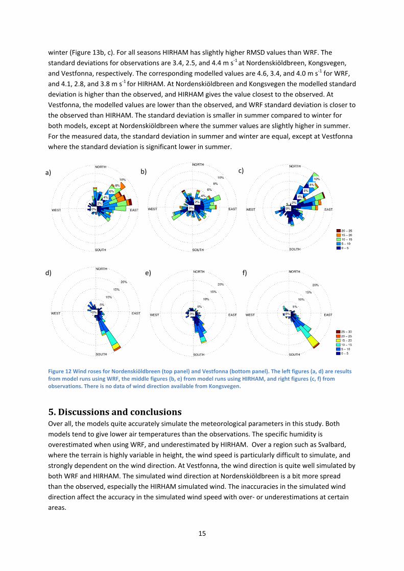
Wind speed and direction at Nordenskiöldbreen and Vestfonna (measured Kongsvegen wind 

direction data were not available) is shown in Figure 12 as wind roses.  Figures (a) and (d) show 

output from WRF, Figures (b) and (e) output from HIRHAM, and Figures (c) and (f) the observed wind. 

The figures show frequencies (%) for wind direction ranges, and wind speed ranges in colors. At 

Nordenskiöldbreen northeast to easterly winds are observed. The maximum wind speed is within the 

range 20‐25 m s‐1. The wind speed is well simulated by WRF, although the spread of wind directions 

a)  b)  c) 

d)  e)  f) 

g)  h)  i) 

14  

is somewhat larger than in the observations. Also, the frequencies with high wind speeds (>15 m s‐1) 

seem to be overestimated. The HIRHAM simulation underestimates the wind speed slightly and the 

wind direction is much more spread out than the observed wind. At Vestfonna the wind direction is 

more uniform with southeasterly winds, and the highest wind speeds are in the range 25‐30 m s‐1.  

The WRF simulated wind has a slightly more southerly direction, and the HIRHAM wind is even 

further towards south. The wind speed from WRF is underestimated, and the highest winds are in 

the range 20‐25 m s‐1. The HIRHAM winds are even more underestimated with maximum winds in 

the range 15‐20 m s‐1.  

        

         

Figure 11 Same as Figure 5 but for specific wind speed (m s‐1). 

The correlation between observed and modeled wind speed is lower than for temperature and 

humidity. The correlation coefficient is within the range 0.74‐0.88 and 0.59‐0.76 for WRF and 

HIRHAM, respectively (Figure 13).  At Nordenskiöldbreen, the correlation is slightly higher in winter 

(R=0.85) than in summer (R=0.81) when using WRF. When using HIRHAM, the correlation is 

approximately equal during winter (R=0.79) and summer (R=0.80) (Figure 13b‐c), and consequently 

somewhat lower than WRF. At Kongsvegen the correlation coefficient is lower in winter than in 

summer for both models, while at Vestfonna the correlation is higher in winter. 

The RMSD values for wind speed are within the range 2.1‐2.8 m s‐1 and 2.4‐2.9 m s‐1 for WRF and 

HIRHAM, respectively (Figure 13). At Kongsvegen and Vestfonna the RMSD value is lower in summer 

(Figure 13e, h) than winter (Figure 13f, i), while at Nordenskiöldbreen RMSD is somewhat lower in 

a)  b) 

c)  d) 

15  

winter (Figure 13b, c). For all seasons HIRHAM has slightly higher RMSD values than WRF. The 

standard deviations for observations are 3.4, 2.5, and 4.4 m s‐1 at Nordenskiöldbreen, Kongsvegen, 

and Vestfonna, respectively. The corresponding modelled values are 4.6, 3.4, and 4.0 m s‐1 for WRF, 

and 4.1, 2.8, and 3.8 m s‐1 for HIRHAM. At Nordenskiöldbreen and Kongsvegen the modelled standard 

deviation is higher than the observed, and HIRHAM gives the value closest to the observed. At 

Vestfonna, the modelled values are lower than the observed, and WRF standard deviation is closer to 

the observed than HIRHAM. The standard deviation is smaller in summer compared to winter for 

both models, except at Nordenskiöldbreen where the summer values are slightly higher in summer. 

For the measured data, the standard deviation in summer and winter are equal, except at Vestfonna 

where the standard deviation is significant lower in summer. 

      

       

Figure 12 Wind roses for Nordenskiöldbreen (top panel) and Vestfonna (bottom panel). The left figures (a, d) are results from model runs using WRF, the middle figures (b, e) from model runs using HIRHAM, and right figures (c, f) from observations. There is no data of wind direction available from Kongsvegen. 

5.DiscussionsandconclusionsOver all, the models quite accurately simulate the meteorological parameters in this study. Both 

models tend to give lower air temperatures than the observations. The specific humidity is 

overestimated when using WRF, and underestimated by HIRHAM.  Over a region such as Svalbard, 

where the terrain is highly variable in height, the wind speed is particularly difficult to simulate, and 

strongly dependent on the wind direction. At Vestfonna, the wind direction is quite well simulated by 

both WRF and HIRHAM. The simulated wind direction at Nordenskiöldbreen is a bit more spread 

than the observed, especially the HIRHAM simulated wind. The inaccuracies in the simulated wind 

direction affect the accuracy in the simulated wind speed with over‐ or underestimations at certain 

areas.  

c) a)  b) 

d)  e)  f) 

16  

         

       

            

Figure 13 Taylor diagrams as Figure 7 but for wind speed.  

Although there are significant differences between simulated and observed wind speed, the 

variability in the wind speed is quite well captured. The ability to accurately simulate the wind will 

also affect other meteorological parameters, although discrepancies between the models occur also 

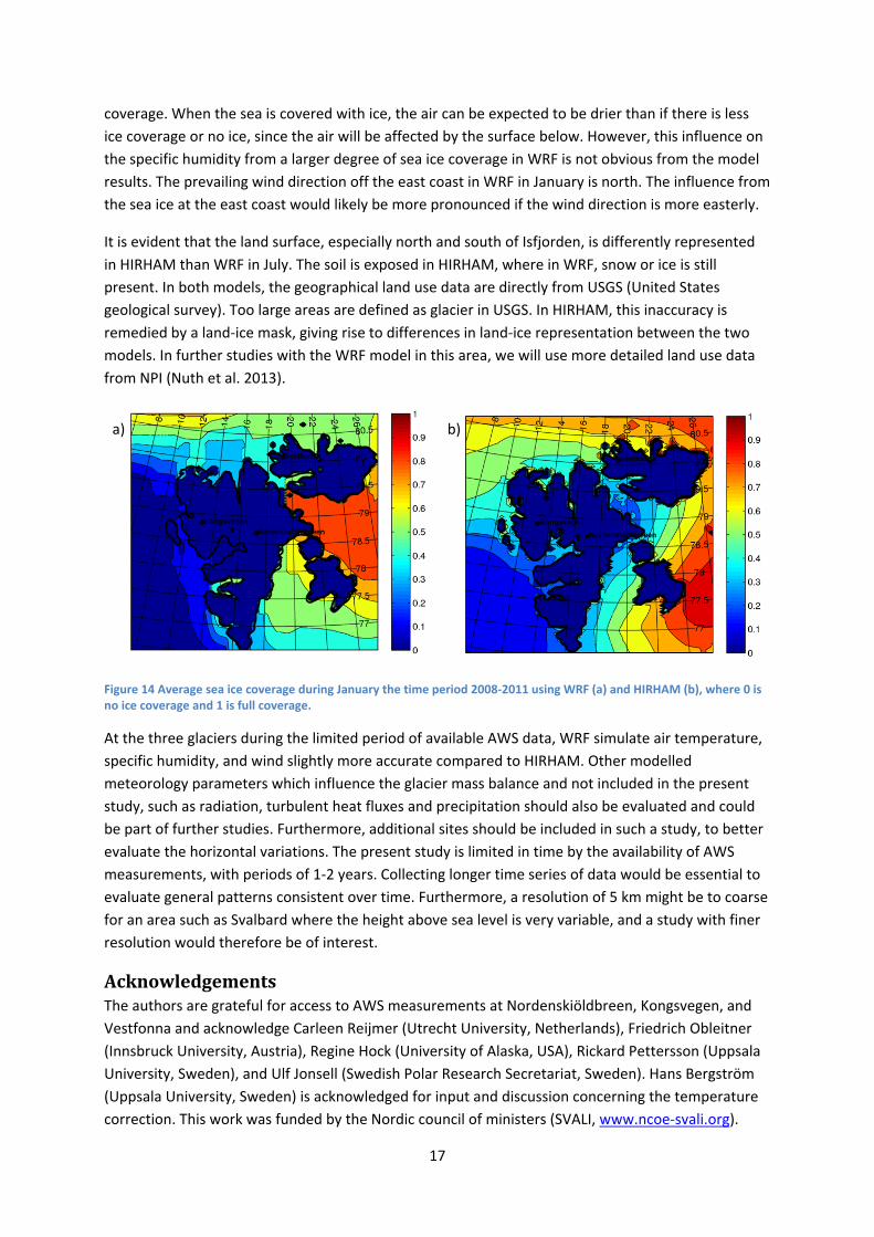
for other reasons such as different physics schemes, or different methods of downscaling. In both 

models ERA interim data of sea ice is used as input, although in the finer resolution, the sea ice is 

interpolated in different ways in WRF and HIRHAM, resulting in differences in the 5.5 km resolution 

sea ice coverage as shown in Figure 14. The most noticeable differences between the models are 

east of Spitsbergen, Isfjorden, and south and north of Nordaustlandet. At the east coast of 

Spitsbergen, there is larger ice coverage in WRF than in HIRHAM. In WRF there is open water in 

Isfjorden, while HIRHAM give some degree of ice coverage. Whether or not the sea is ice covered 

should strongly influence the turbulent heat fluxes and radiation, and will thus affect the air 

temperature and humidity. Studying the air temperature in January (Figure 5), it is noticeable that 

the air temperature over the ocean is colder in WRF than in HIRHAM, although, the temperature 

over land at the east coast in WRF does not seem to be influenced by the higher degree of sea ice 

a)  b)  c) 

d)  e)  f) 

g)  h)  i) 

17  

coverage. When the sea is covered with ice, the air can be expected to be drier than if there is less 

ice coverage or no ice, since the air will be affected by the surface below. However, this influence on 

the specific humidity from a larger degree of sea ice coverage in WRF is not obvious from the model 

results. The prevailing wind direction off the east coast in WRF in January is north. The influence from 

the sea ice at the east coast would likely be more pronounced if the wind direction is more easterly. 

It is evident that the land surface, especially north and south of Isfjorden, is differently represented 

in HIRHAM than WRF in July. The soil is exposed in HIRHAM, where in WRF, snow or ice is still 

present. In both models, the geographical land use data are directly from USGS (United States 

geological survey). Too large areas are defined as glacier in USGS. In HIRHAM, this inaccuracy is 

remedied by a land‐ice mask, giving rise to differences in land‐ice representation between the two 

models. In further studies with the WRF model in this area, we will use more detailed land use data 

from NPI (Nuth et al. 2013). 

              

Figure 14 Average sea ice coverage during January the time period 2008‐2011 using WRF (a) and HIRHAM (b), where 0 is no ice coverage and 1 is full coverage. 

At the three glaciers during the limited period of available AWS data, WRF simulate air temperature, 

specific humidity, and wind slightly more accurate compared to HIRHAM. Other modelled 

meteorology parameters which influence the glacier mass balance and not included in the present 

study, such as radiation, turbulent heat fluxes and precipitation should also be evaluated and could 

be part of further studies. Furthermore, additional sites should be included in such a study, to better 

evaluate the horizontal variations. The present study is limited in time by the availability of AWS 

measurements, with periods of 1‐2 years. Collecting longer time series of data would be essential to 

evaluate general patterns consistent over time. Furthermore, a resolution of 5 km might be to coarse 

for an area such as Svalbard where the height above sea level is very variable, and a study with finer 

resolution would therefore be of interest. 

AcknowledgementsThe authors are grateful for access to AWS measurements at Nordenskiöldbreen, Kongsvegen, and 

Vestfonna and acknowledge Carleen Reijmer (Utrecht University, Netherlands), Friedrich Obleitner 

(Innsbruck University, Austria), Regine Hock (University of Alaska, USA), Rickard Pettersson (Uppsala 

University, Sweden), and Ulf Jonsell (Swedish Polar Research Secretariat, Sweden). Hans Bergström 

(Uppsala University, Sweden) is acknowledged for input and discussion concerning the temperature 

correction. This work was funded by the Nordic council of ministers (SVALI, www.ncoe‐svali.org). 

a)  b) 

18  

ReferencesChristensen, J.H., O. B. Christensen, P. Lopez, E. van Meijgaard, and M. Botzet (1996): The HIRHAM4 

regional atmospheric climate model. DMI Scientific Report 96‐4, Danish 

Meteorological Institute, Kopenhagen, Denmark. 

Christensen, O.B., M. Drews, and J.H. Christensen (2007): The HIRHAM Regional Climate Model 

Version 5(β). Technical report 06‐17, Danish Meteorological Institute, Kopenhagen, 

Denmark. 

Claremar, B., F. Obleitner, C. Reijmer, V. Pohjola, A. Waxegård, F. Karner, and A. Rutgersson (2012): 

Applying a Mesoscale Atmospheric Model to Svalbard Glaciers. Advances in 

Meteorology, 321649. Doi: 10.1155/2012/321649. 

Claremar, B. (2013): Water retention parameterization in the WRF model – A sensitivity test. SVALI 

Deliverable D3.1‐1 report, Uppsala University, Uppsala, Sweden. 

Dee, D.P. S.M. Uppala, A.J. Simmons, P. Berrisford, P. Poli, S. Kobayashi, U. Andrae, M.A. Balmaseda, 

G. Balsamo, P. Bauer, P. Bechtold, A.C.M. Beljaars, L. van de Berg, J. Bidlot, N. 

Bormann, C. Delsol, R. Dragani, M. Fuentes, A.J. Geer, L. Haimberger, S.B. Healy, H. 

Hersbach, E.V. Hólm, L. Isaksen, P. Kållberg, M. Köhler, M. Matricardi, A.P. McNally, 

B.M. Monge‐Sanz, J.J. Morcrette, B.K. Park, C. Peubey, P. de Rosnay, C. Tavolato, J.N. 

Thépaut, F. Vitart (2011): The ERA‐Interim reanalysis: configuration and performance 

of the data assimilation system. Q.J.R. Meteorol. Soc., 137:553‐597. Doi: 

10.1002/qj.828. 

den Ouden, M.A.G., C.H. Reijmer, V. Pohjola, R.S.W. van de Wal, J. Oerlemans, and W. Boot (2010): 

Stand‐alone single‐frequency GPS ice velocity observations on Nordenskiöldbreen, 

Svalbard. Cryosphere, 4(4), 593‐604. 

Hines, K.M., and D.H. Bromwich (2008): Development and testing of polar weather research and 

forecasting (WRF) model. Part I: Greenland ice sheet meteorology. Monthly Weather 

Review, 136(6):1971‐1989. 

Möller, M., R. Finkelburg, M. Braun et al. (2011): Climatic mass balance of the ice cap Vestfonna, 

Svalbard: a spatially distrubuted assessment using ERA‐Interim and MODIS data. J. 

Geophys. Res., 116:1‐14. 

Nuth, C., J. Kohler, M.  König, A. von Deschwanden, J.O. Hagen, A. Kääb,G.  Mohold, and R. Pettersson 

(2013): Decadal changes from a multi‐temporal glacier inventory of Svalbard. The 

Cryosphere, 7, 1603‐1621, doi:10.5194/tc‐7‐1603‐2013. 

Obleitner, F., and M. Lehning (2004): Measurement and simulation of snow and superimposed ice at 

the Kongsvegen glacier, Svalbard (Spitzbergen). J. Geophys. Res. D, 109(4):1‐12. 

Pohjola, V. A., P. Kankaanpää, J. C. Moore, and T.Pastusiak (2011): Preface: the international polar 

year project “Kinnevika” – arctic warming and impact research at 80 N. Geografiska 

Annaler , 93A(4): 201‐208. 

19  

Pohjola, V.A., J.C. Moore, E. Isaksson et al. (2002): Effect of periodic melting on geochemical and 

isotopic signals in an ice core from Lomonosovfonna, Svalbard. J. Geophys. Res., 

107(4):1‐14. 

Roeckner, E., G. Bäuml, L. Bonaventura, R. Brokopf, M. Esch, M. Giorgetta, S. Hagemann, I. Kirchner, 

L. Kornblueh, E. Manzini, A. Rhodin, U. Schlese, U. Schulzweida, and A. Tompkins 

(2003): The atmospheric general circulation model ECHAM 5. PART I: Model 

description. MPI‐Report No. 349, Max Planck Institute for Meteorology, Hamburg, 

Germany. 

Skamarock, W. C., and J. B. Klemp (2008): A time‐split non‐hydrostatic atmospheric model for weather research and forecasting applications. J. Comput. Phys., 227, 3465–3485. 

 Sterns, C. R., G.A. Weidner, and L.M. Keller (1997): Atmospheric circulation around the Greenland 

Crest. J. Geophys. Res., 102:13801‐13812.  Taylor, K. E., (2001): Summarizing multiple aspects of model performance in a single diagram. J. 

Geophys. Res., 106, 7183‐7192.  Undén, P., L. Rontu, H. Järvinen, P. Lynch, J. Calvo, G.Cats, J. Cuxart, K. Erola, C. Fortelius, J.A. Garcia‐

Moya, C. Jones, G. Lenderlink, A. McDonald, R. McGrath, B. Navascues, N.W. Nielsen, V. Ødegaard, E. Rodriguez, M. Rummukainen, R. Rõõm, K. Sattler, B.H. Sass, H Savijärvi, B.W. Schreur, R. Sigg, H. The, and A. Tijm (2002): HIRLAM‐5 Scientific Documentation, Swedish Meteorological and Hydrological Institute (SMHI), Norrköping, Sweden. 

 Van Pelt, W.J.J., J. Oerlemans, C.H. Reijmer, V.A. Pohjala, R. Pettersson, and J.H. van Angelen (2011): 

Simulating melt, runoff and refreezing on Nordenskiöldbreen, Svalbard, using a 

coupled snow and energy balance model. The Cryosphere Discussions, 6, 211‐266. 

Vaughan, D.G., J.C. Comiso, I. Allison, J. Carrasco, G. Kaser, R. Kwok, P. Mote, T. Murray, F. Paul, J. Ren, E. Rignot, O. Solomina, K. Steffen and T. Zhang (2013): Observations: Cryosphere. In: Climate Change 2013: The Physical Science Basis. Contribution of Working Group I to the Fifth Assessment Report of the Intergovernmental Panel on Climate Change [Stocker, T.F., D. Qin, G.‐K. Plattner, M. Tignor, S.K. Allen, J. Boschung, A. Nauels, Y. Xia, V. Bex and P.M. Midgley (eds.)]. Cambridge University Press, Cambridge, United Kingdom and New York, NY, USA.