continuous probabilistic subspace skyline query processing using grid projections

Zhao L, Yang YY, Zhou X. Continuous probabilistic subspace skyline query processing using grid projections. JOURNAL

OF COMPUTER SCIENCE AND TECHNOLOGY 29(2): 332–344 Mar. 2014. DOI 10.1007/s11390-014-1434-9

Continuous Probabilistic Subspace Skyline Query Processing Using

Grid Projections

Lei Zhao1 (赵雷), Member, CCF, ACM, Yan-Yan Yang2 (杨艳艳)and Xiaofang Zhou1,3 (周晓方), Member, CCF, ACM, IEEE

1School of Computer Science and Technology, Soochow University, Suzhou 215006, China2Open System& Storage Interoperability Test Laboratory, IBM, Wuxi 214000, China3School of Information Technology and Electrical Engineering, The University of Queensland, Brisbane, QLD 4072, Australia

E-mail: [email protected]; [email protected]; [email protected]

Received September 4, 2013; revised December 16, 2013.

Abstract As an important type of multidimensional preference query, the skyline query can find a superset of optimalresults when there is no given linear function to combine values for all attributes of interest. Its processing has beenextensively investigated in the past. While most skyline query processing algorithms are designed based on the assumptionthat query processing is done for all attributes in a static dataset with deterministic attribute values, some advanced workhas been done recently to remove part of such a strong assumption in order to process skyline queries for real-life applications,namely, to deal with data with multi-valued attributes (known as data uncertainty), to support skyline queries in a subspacewhich is a subset of attributes selected by the user, and to support continuous queries on streaming data. Naturally, thereare many application scenarios where these three complex issues must be considered together. In this paper, we tackle theproblem of probabilistic subspace skyline query processing over sliding windows on uncertain data streams. That is, toretrieve all objects from the most recent window of streaming data in a user-selected subspace with a skyline probability nosmaller than a given threshold. Based on the subtle relationship between the full space and an arbitrary subspace, a novelapproach using a regular grid indexing structure is developed for this problem. An extensive empirical study under varioussettings is conducted to show the effectiveness and efficiency of our PSS algorithm.

Keywords probabilistic query, continuous query, subspace, skyline

1 Introduction

Skyline query has received considerable attention indatabases[1-4]. It is used to find a set of non-dominatedobjects in a multidimensional dataset. An object oidominates another object oj if and only if oi is as goodas oj in all dimensions and it is better than oj in atleast one of the dimensions.

Recently, the skyline query has been further ap-plied on uncertain streaming data to provide advancedanalysis for some important applications, such as mar-ket surveillance and sensor networks. Due to the un-certainty, the dominance relationships between objectsbecome uncertain and come with a probability value.However, only full dimensional skyline queries are con-sidered in previous work. Since different users maybe interested in different dimensions, subspace skylinequeries are much more practical in many applicationdomains.

1.1 Motivation

In [5], the on-line products selection problem ismodeled as probabilistic skyline against sliding windowby regarding on-line advertisements as a data stream.All products are described by their attributes such asbrand, price, size, weight, and quality. Once a trans-action finishes, the customer is usually encouraged torate the seller’s performance. Therefore, each seller isassociated with a reputation value formulated by itscustomers’ feedback. The seller reputation representsthe probability of occurrence that the product occursin the on-line advertisement. It also helps determinewhether a transaction will occur and how parties willbehave. Customers may want to monitor on-line ad-vertisements by selecting the candidates, whose prob-ability of skyline on the full space is larger than thethreshold q, for the best deal-skyline points. This kindof skyline query can be called q-skylines on full space.

Regular PaperThis work is supported by the National Natural Science Foundation of China under Grant Nos. 61073061, 61003044, 61303019,

and the Natural Science Foundation of Colleges and Universities of Jiangsu Province of China under Grant No. 12KJB520017.©2014 Springer Science+Business Media, LLC & Science Press, China

Lei Zhao et al.: Continuous Probabilistic Subspace Skyline 333

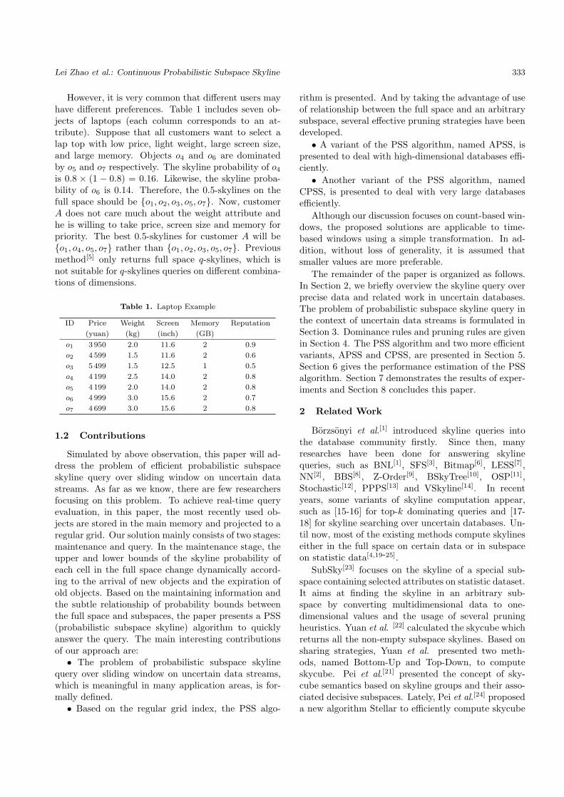
However, it is very common that different users mayhave different preferences. Table 1 includes seven ob-jects of laptops (each column corresponds to an at-tribute). Suppose that all customers want to select alap top with low price, light weight, large screen size,and large memory. Objects o4 and o6 are dominatedby o5 and o7 respectively. The skyline probability of o4is 0.8 × (1 − 0.8) = 0.16. Likewise, the skyline proba-bility of o6 is 0.14. Therefore, the 0.5-skylines on thefull space should be {o1, o2, o3, o5, o7}. Now, customerA does not care much about the weight attribute andhe is willing to take price, screen size and memory forpriority. The best 0.5-skylines for customer A will be{o1, o4, o5, o7} rather than {o1, o2, o3, o5, o7}. Previousmethod[5] only returns full space q-skylines, which isnot suitable for q-skylines queries on different combina-tions of dimensions.

Table 1. Laptop Example

ID Price Weight Screen Memory Reputation

(yuan) (kg) (inch) (GB)

o1 3 950 2.0 11.6 2 0.9

o2 4 599 1.5 11.6 2 0.6

o3 5 499 1.5 12.5 1 0.5

o4 4 199 2.5 14.0 2 0.8

o5 4 199 2.0 14.0 2 0.8

o6 4 999 3.0 15.6 2 0.7

o7 4 699 3.0 15.6 2 0.8

1.2 Contributions

Simulated by above observation, this paper will ad-dress the problem of efficient probabilistic subspaceskyline query over sliding window on uncertain datastreams. As far as we know, there are few researchersfocusing on this problem. To achieve real-time queryevaluation, in this paper, the most recently used ob-jects are stored in the main memory and projected to aregular grid. Our solution mainly consists of two stages:maintenance and query. In the maintenance stage, theupper and lower bounds of the skyline probability ofeach cell in the full space change dynamically accord-ing to the arrival of new objects and the expiration ofold objects. Based on the maintaining information andthe subtle relationship of probability bounds betweenthe full space and subspaces, the paper presents a PSS(probabilistic subspace skyline) algorithm to quicklyanswer the query. The main interesting contributionsof our approach are:

• The problem of probabilistic subspace skylinequery over sliding window on uncertain data streams,which is meaningful in many application areas, is for-mally defined.

• Based on the regular grid index, the PSS algo-

rithm is presented. And by taking the advantage of useof relationship between the full space and an arbitrarysubspace, several effective pruning strategies have beendeveloped.

• A variant of the PSS algorithm, named APSS, ispresented to deal with high-dimensional databases effi-ciently.

• Another variant of the PSS algorithm, namedCPSS, is presented to deal with very large databasesefficiently.

Although our discussion focuses on count-based win-dows, the proposed solutions are applicable to time-based windows using a simple transformation. In ad-dition, without loss of generality, it is assumed thatsmaller values are more preferable.

The remainder of the paper is organized as follows.In Section 2, we briefly overview the skyline query overprecise data and related work in uncertain databases.The problem of probabilistic subspace skyline query inthe context of uncertain data streams is formulated inSection 3. Dominance rules and pruning rules are givenin Section 4. The PSS algorithm and two more efficientvariants, APSS and CPSS, are presented in Section 5.Section 6 gives the performance estimation of the PSSalgorithm. Section 7 demonstrates the results of exper-iments and Section 8 concludes this paper.

2 Related Work

Borzsonyi et al.[1] introduced skyline queries intothe database community firstly. Since then, manyresearches have been done for answering skylinequeries, such as BNL[1], SFS[3], Bitmap[6], LESS[7],NN[2], BBS[8], Z-Order[9], BSkyTree[10], OSP[11],Stochastic[12], PPPS[13] and VSkyline[14]. In recentyears, some variants of skyline computation appear,such as [15-16] for top-k dominating queries and [17-18] for skyline searching over uncertain databases. Un-til now, most of the existing methods compute skylineseither in the full space on certain data or in subspaceon statistic data[4,19-25].

SubSky[23] focuses on the skyline of a special sub-space containing selected attributes on statistic dataset.It aims at finding the skyline in an arbitrary sub-space by converting multidimensional data to one-dimensional values and the usage of several pruningheuristics. Yuan et al. [22] calculated the skycube whichreturns all the non-empty subspace skylines. Based onsharing strategies, Yuan et al. presented two meth-ods, named Bottom-Up and Top-Down, to computeskycube. Pei et al.[21] presented the concept of sky-cube semantics based on skyline groups and their asso-ciated decisive subspaces. Lately, Pei et al.[24] proposeda new algorithm Stellar to efficiently compute skycube

334 J. Comput. Sci. & Technol., Mar. 2014, Vol.29, No.2

without enumerating all the possible subspaces. It firstcomputes seed skyline groups in the full space, and thenextends them to shape the final set of skyline groups.Recently, Raissi et al.[25] developed more efficient algo-rithms to compute the closed subspaces based on formalconcept analysis.

The skyline query processing on uncertain data wasfirstly defined by Pei et al.[26], and two techniques weredeveloped for efficient computation. Lian et al.[17] com-bined reverse skylines with uncertain semantics andmodeled the probabilistic reverse skyline query. Zhanget al.[5] explored an efficient algorithm, maintainingminimum candidate set by using aggregate R-tree, toanswer continuous probabilistic skyline query. Atallahet al.[27] tackled the problem of computing all skylineprobabilities for every object.

Since probabilistic subspace skyline query on uncer-tain data streams is different from all those problemsaddressed in the forementioned papers, techniques pro-posed in those papers cannot be adapted directly to theproblem addressed in this paper.

3 Problem Definition

In this section, we will give the problem descriptionof probabilistic subspace skyline query and a straight-forward method. Table 2 lists the notations used in thispaper.

Table 2. Summary of Notations

Notation Definition

O Object set of current window

Ci A cell of the regular grid index, denoted as

(c1i , c2i , . . . , c

|D|i )

Oi Object set of cell CiD Full space, denoted as (d1, d2,. . . , d|D|)B A non-empty subspace

πCi→B Projection of a cell Ci in subspace Bωo Occurrence probability of object o

$o Non-dominated probability of object o

κo Probability of being probabilistic skyline pointof object o

q Threshold probability given by the user

G Number of grid cells per dimension

τminCi

, τmaxCi

Lower-left/upper-right corner of cell Ci$Ci

Non-dominated probability of Ci$min

Ci, $max

CiMinimum/maximum non-dominated probabi-lity of Ci

Assume full space D = {d1, d2, . . . , dn} and all ob-jects in current window O = {o1, o2, . . . , o|O|}. In apossible world, the probability of an object o being askyline object can be verified by (1):

κo = ωo ×$o, (1)

where$o =

∏

o′∈O,o′≺o

(1− ωo′). (2)

So, the problem of probabilistic subspace skylinequery on data streams can be described as follows:

• Suppose, O is the set of all objects in current win-dow and each object has a probability of occurrence.

• A non-empty subspace B ⊆ D and a threshold q(0 < q 6 1) are given.

• The query retrieves a subset O′ from O in subspaceB, satisfying κo > q (o ∈ O′), where notation κ meansthe probability of an object being a skyline object.

A straightforward solution to this problem can bedesigned as follows: whenever users submit their in-terested subspaces and threshold q, each uncertain ob-ject computes with all the other objects contained inthe current window to obtain its skyline probability.This method will cause O(|O|2) dominance tests. Asour experiments will report in Subsection 7.1, this kindof straightforward method takes about 70 seconds tocompute the 0.3-skyline on 5-dimensional (5D) datasetwith anti-correlated distribution and the window size isjust 100K. Obviously, this solution is very costly. It isnecessary to devise more efficient methods to computeprobabilistic skyline on data streams for any given sub-space.

The key of any efficient skyline algorithm is to elimi-nate objects which are not in the skyline as quicklyas possible. Our solution is no exception. Instead ofcomputing skyline in the object level directly, we em-ploy grid index and make possible elimination in coarsergrained level first. We get the upper and lower boundsof the non-dominated probability of each cell. It helpsto determine which objects can be pruned directly. R-tree is also a popular index, but it is not adopted inthis work because R-tree needs 2|D| − 1 times of pre-computing.

This work is to solve continuous queries. Similar to[28], objects in sliding window are evicted in an FIFOmanner. The insertion and deletion also occur in thesame way.

Definition 1 (Grid Cell). Given a full space D =(d1, d2, . . . , d|D|), suppose each dimension is evenly di-vided into G segments and number all of these segmentsfrom 1 to G, then the full space is cut into G|D| gridcells. Each of them can be named by a sequence of |D|numbers, denoted as C = (c1, c2, . . . , c|D|), where cx isthe segment number of the x-th dimension.

Definition 2 (Lower-Left Corner). Given a cell C,the lower-left corner is the point in C which has the min-imum coordinates in all dimensions, denoted as τmin

C .Definition 3 (Upper-Right Corner). Given a cell

C, the upper-right corner is the point in C which has


the maximum coordinates in all dimensions, denoted asτmaxC .Lemma 1. Given Ci = (c1i , c

2i , . . . , c

|D|i ), if ∀x

(1 6 x 6 |D|), it follows cxi > 1, then τmin

(c1i ,c2i ,...,c

|D|i )

=

τmax

(c1i−1,c2i−1,...,c|D|i −1)

.

Proof. Suppose, ∀x (1 6 x 6 |D|), the value of dxfalls in the range of [0,maxx].

According to Definition 1, it is easy to see that thex-th coordinate of τmin

(c1i ,c2i ,...)

is

cxi × maxxG .

Similarly, we have the x-th coordinate of τmax(c1i−1,c2i−1,...)

as:(cxi − 1)× maxx

G +maxxG = cxi × maxx

G .

Therefore,

τmin

(c1i ,c2i ,...,c

|D|i )

= τmax

(c1i−1,c2i−1,...,c|D|i −1)

. ¤

4 Derivation Rules

In this section, we first present some dominance rulesderived by the regular grid, then propose some pruningstrategies that will be used in the PSS algorithm.

4.1 Dominance Rules

Based on the principle of SFS[3], it is easy to getDefinitions 4∼6.

Definition 4 (Full Dominating). Given two cells C1and C2, if ∀di ∈ D, it follows that τmin

C1→di< τmin

C2→di,

then C1 fully dominates C2, denoted as C1 ≺ C2.Definition 5 (Partially Dominating). Given two

cells C1 and C2, if ∃B ⊂ D, for which ∀di ∈ B, it fol-lows that τmin

C1→di= τmin

C2→diand ∀dj ∈ D − B, it follows

that τminC1→dj

< τminC2→dj

, then C1 partially dominates C2,denoted as C1 / C2.

Definition 6 (Non-Dominating). Given two cells C1and C2, if ∃di ∈ D, for which τmin

C1→di> τmin

C2→di, then C1

does not dominate C2, denoted as C1 6≺ C2.According to Definitions 4∼6, Lemma 2 can be eas-

ily verified.Lemma 2. ∀oi ∈ Ci and ∀oj ∈ Cj, oi and oj must

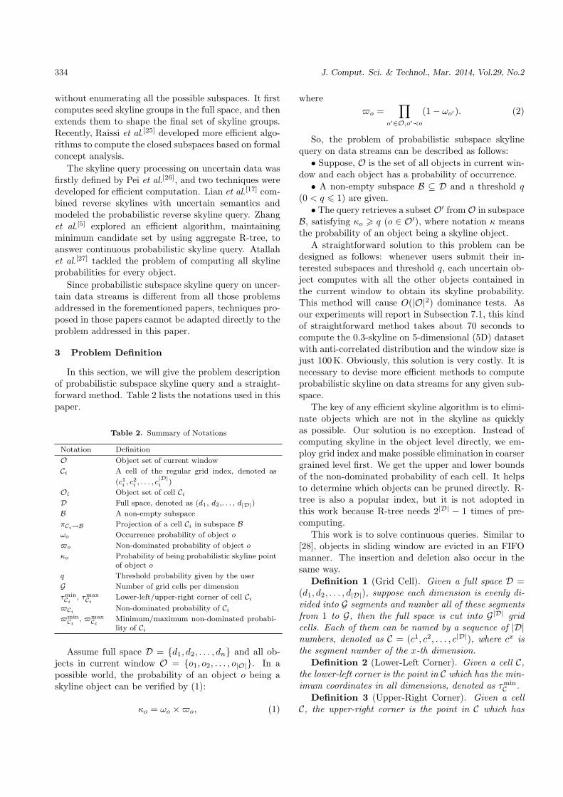
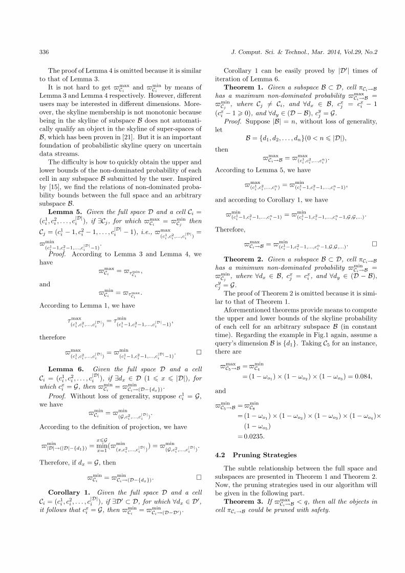
have one of the following relations:1) Ci ≺ Cj ⇒ oi ≺ oj,2) Ci / Cj 6⇒ oi ≺ oj,3) Ci 6≺ Cj ⇒ oi 6≺ oj and oj 6≺ oi.Consider a set of uncertain objects in Fig.1, where

the occurrence probability of each object is given andthe full space D = {d1, d2}. Take C6 for example, C6 isfully dominated by C1 and it is partially dominated by

C2 and C5. Thus,

$maxC6

= 1− ωo1 = 0.2,

and

$minC6

= (1− ωo1)× (1− ωo2)× (1− ωo5) = 0.084.

Fig.1. Set of uncertain objects.

In the context, Ci means Ci is in the full space bydefault. Lemma 2 also applies to any subspace and iscritical in this work. By means of Lemma 2, we employthe upper and lower bounds of non-dominated proba-bility of each cell in the full space.

Definition 7 (Upper Bound of $Ci). The upper

bound of non-dominated probability of Ci, denoted as$max

Ci, is the probability that ∀o ∈ Ci, it follows that

$o 6 $maxCi

.Lemma 3. Given Ci, then the upper bound of non-

dominated probability of Ci is $maxCi

= $τminCi

.Proof. Given an object o ∈ Ci, if ∃o′ ∈ C′, for which

o′ ≺ o, then there exists three possibilities:1) C′ ≺ Ci,2) C′ / Ci,3) C′ = Ci.The first possibility cannot be avoided, but the sec-

ond and the third one can. According to Definition 2,τminCi

is the only point which guarantees the avoidanceof the second and the third possibility. Therefore,

$maxCi

= $τminCi

. ¤

Definition 8 (Lower Bound of $Ci). The lower

bound of non-dominated probability of Ci, denoted as$min

Ci, is the probability that ∀o ∈ Ci, it follows $o >

$minCi

.Lemma 4. Given Ci, then the lower bound of non-

dominated probability of Ci is $minCi

= $τmaxCi

.


The proof of Lemma 4 is omitted because it is similarto that of Lemma 3.

It is not hard to get $maxCi

and $minCi

by means ofLemma 3 and Lemma 4 respectively. However, differentusers may be interested in different dimensions. More-over, the skyline membership is not monotonic becausebeing in the skyline of subspace B does not automati-cally qualify an object in the skyline of super-spaces ofB, which has been proven in [21]. But it is an importantfoundation of probabilistic skyline query on uncertaindata streams.

The difficulty is how to quickly obtain the upper andlower bounds of the non-dominated probability of eachcell in any subspace B submitted by the user. Inspiredby [15], we find the relations of non-dominated proba-bility bounds between the full space and an arbitrarysubspace B.

Lemma 5. Given the full space D and a cell Ci =(c1i , c

2i , . . . , c

|D|i ), if ∃Cj, for which $max

Ci= $min

Cjthen

Cj = (c1i − 1, c2i − 1, . . . , c|D|i − 1), i.e., $max

(c1i ,c2i ,...,c

|D|i )

=

$min

(c1i−1,c2i−1,...,c|D|i −1)

.

Proof. According to Lemma 3 and Lemma 4, wehave

$maxCi

= $τminCi

,

and$min

Ci= $τmax

Ci.

According to Lemma 1, we have

τmax

(c1i ,c2i ,...,c

|D|i )

= τmin

(c1i−1,c2i−1,...,c|D|i −1)

,

therefore

$max

(c1i ,c2i ,...,c

|D|i )

= $min

(c1i−1,c2i−1,...,c|D|i −1)

. ¤

Lemma 6. Given the full space D and a cellCi = (c1i , c

2i , . . . , c

|D|i ), if ∃dx ∈ D (1 6 x 6 |D|), for

which cxi = G, then $minCi

= $minCi→(D−{dx}).

Proof. Without loss of generality, suppose c1i = G,we have

$minCi

= $min

(G,c2i ,...,c|D|i )

.

According to the definition of projection, we have

$min|D|→(|D|−{d1}) =

x6Gminx=1

($min

(x,c2i ,...,c|D|i )

) = $min

(G,c2i ,...,c|D|i )

.

Therefore, if dx = G, then

$minCi

= $minCi→(D−{dx}). ¤

Corollary 1. Given the full space D and a cellCi = (c1i , c

2i , . . . , c

|D|i ), if ∃D′ ⊂ D, for which ∀dx ∈ D′,

it follows that cxi = G, then $minCi

= $minCi→(D−D′).

Corollary 1 can be easily proved by |D′| times ofiteration of Lemma 6.

Theorem 1. Given a subspace B ⊂ D, cell πCi→Bhas a maximum non-dominated probability $max

Ci→B =$min

Cj, where Cj 6= Ci, and ∀dx ∈ B, cxj = cxi − 1

(cxi − 1 > 0), and ∀dy ∈ (D − B), cyj = G.Proof. Suppose |B| = n, without loss of generality,

letB = {d1, d2, . . . , dn}(0 < n 6 |D|),

then$max

Ci→B = $max(c1i ,c

2i ,...,c

ni ).

According to Lemma 5, we have

$max(c1i ,c

2i ,...,c

ni )

= $min(c1i−1,c2i−1,...,cni −1),

and according to Corollary 1, we have

$min(c1i−1,c2i−1,...,cni −1) = $min

(c1i−1,c2i−1,...,cni −1,G,G,...).

Therefore,

$maxCi→B = $min

(c1i−1,c2i−1,...,cni −1,G,G,...). ¤

Theorem 2. Given a subspace B ⊂ D, cell πCi→Bhas a minimum non-dominated probability $min

Ci→B =$min

Cj, where ∀dx ∈ B, cxj = cxi , and ∀dy ∈ (D − B),

cyj = G.The proof of Theorem 2 is omitted because it is simi-

lar to that of Theorem 1.Aforementioned theorems provide means to compute

the upper and lower bounds of the skyline probabilityof each cell for an arbitrary subspace B (in constanttime). Regarding the example in Fig.1 again, assume aquery’s dimension B is {d1}. Taking C5 for an instance,there are

$maxC5→B =$min

C4

=(1− ωo1)× (1− ωo2)× (1− ωo3) = 0.084,

and

$minC5→B =$min

C8

=(1− ωo1)× (1− ωo2)× (1− ωo3)× (1− ωo4)×(1− ωo5)

= 0.0235.

4.2 Pruning Strategies

The subtle relationship between the full space andsubspaces are presented in Theorem 1 and Theorem 2.Now, the pruning strategies used in our algorithm willbe given in the following part.

Theorem 3. If $maxCi→B < q, then all the objects in

cell πCi→B could be pruned with safety.


Proof. According to Definition 7, we have ∀o ∈πCi→B, it follows that

$o 6 $maxCi→B < q.

The occurrence probability of o is

ωo 6 1,

and it follows that

κo = ωo ×$o < q.

Therefore, any object in cell πCi→B must not be in theskyline. ¤

Theorem 4. If $minCi→B > q, and ∃o ∈ πCi→B, for

which ωo ×$minCi→B > q, then o must be in the skyline.

The proof of Theorem 4 is similar to that of Theo-rem 3. Based on the pruning strategies, lots of objectscan be pruned quickly without dominance tests.

For example, consider the situation in Fig.1, and letq = 0.5. Because $max

C5→B = 0.084 < q, all the objectsin πC5→B are not skyline points according to Theorem3. Similarly, objects in the cells from C5 to C16 can bepruned. Those objects in the cells from C1 to C4 need tobe checked accurately since they are not qualified withTheorem 3 and Theorem 4.

If an object o is in the skyline, it is theoreticallynecessary to be compared with all the objects which arecontained in the cells that fully and partially dominatethe cell hosting o. While in PSS, it just needs to com-pare o with the objects which are contained in the cellspartially dominating the cell hosting o, for $max

C (o ∈ C)can be easily derived by Theorem 1. In addition, inorder to further reduce dominance tests cost, a heap isemployed to keep the result of dominance tests betweenobjects in the same cell to avoid repeated comparisons.Moreover, the space consumption is very small.

5 PSS Algorithm

5.1 Baseline PSS Computation

Take the dataset in Fig.1 for example, assume that anew subspace query B = {d1} is submitted by the userwith probability threshold q = 0.3. The PSS algorithmwill execute in the following steps.

1) PSS first projects each cell Ci in subspace B to getπCi→B, and then reorganizes the cells in a special waythat all cells would not have chance to dominate thosecells sorted prior to them. The accessing sequence ofthis query is (πC1→B, πC2→B, . . . , πC15→B, πC16→B).

2) Based on the maintaining information, the PSSalgorithm will figure out the lower and upper boundsof non-dominated probability for each cell in subspace

B using Theorem 1 and Theorem 2. It is easy to get

$maxC1∼4→B = 1.0,

$minC1∼4→B = $min

C4→B = 0.084,

and$max

C5∼16→B 6 $minC4→B.

It follows that

$maxC5∼16→B 6 0.084 < q.

Obviously, the non-dominated probability of each ob-ject in Ci must be in the range of [$min

Ci→B, $maxCi→B]. Now,

it is the time to use Step 3 to evict out the invalid cells.3) According to Theorem 3 and Theorem 4, only

C1 ∼ C4 remain to be candidate cells. The PSS algo-rithm only traverses objects that fall in the remainingcandidate cells. Thus, it is necessary to compute theexact skyline probability of objects in C1 ∼ C4. Thealgorithm terminates, with the skyline of {o1, o2}, afterthe examination of each candidate cell.

The main flow of PSS is given in Algorithm 1. Dur-ing the dominance tests of objects in candidate cells,a temporary heap is employed for saving the result ofcomputed objects and avoiding repeated computing.

Algorithm 1. PSS Query(B, q)1: /* φ means empty set in this paper */

2: S ← φ, H ← φ;

3: Project each Ci in subspace B to get πCi→B;

4: Organize all πCi→B into a sequence, named R, so thatany cell does not have chance to dominate cells sortedprior to them;

5: for each πCi→B ∈ R do

6: if πCi→B 6= φ then

7: Compute $maxCi→B and $min

Ci→B;

8: if $maxCi→B < q then

9: Continue;

10: else

11: Get-Candidate();

12: Get-Skyline();

13: end if

14: end if

15: end for

16: Return S;

Algorithm 2 and Algorithm 3 describe the methodof getting candidate cells and of digging the skyline outof all objects in candidate cells, respectively.

5.2 Updating

The PSS algorithm keeps all objects in the currentwindow until their expiration, which is different from


Algorithm 2. Get-Candidate()

1: H ← φ;

2: for each o ∈ πCi→B do

3: $o ← $maxCi→B;

4: if H = φ then

5: H ← H+ {o};6: else

7: for each o′ ∈ H do

8: if o ≺ o′ then

9: $o′ ← $o′ × (1− ωo);

10: end if

11: if o′ ≺ o then

12: $o ← $o × (1− ωo′);

13: end if

14: if $o′ < q then

15: H ← H− {o′};16: end if

17: if $o < q then

18: Break;

19: end if

20: end for

21: if $o q then

22: H ← H+ {o};23: end if

24: end if

25: end for

Algorithm 3. Get-Skyline()

1: for each o ∈ H do

2: $o = $o × ωo;

3: if $o < q then

4: Continue;

5: else

6: for each Cj (o ∈ Ci, Cj ∈ R, j < i, Cj / Ci) do

7: for each o′ ∈ Cj and o′ ≺ o do

8: $o = $o × (1− ωo′);

9: if $o < q then

10: Continue;

11: end if

12: end for

13: end for

14: S ← S + {o};15: end if

16: end for

[5]. This is because the threshold of probability comesfrom different users and it is not fixed.

In the maintenance stage, the algorithm first findsout the cell Ci that the new arrival object o (or old ex-piring object) belongs to. Then, changes the lower andupper bounds of skyline probability for each cell whichis dominated by o. All the maintaining information is

based on the full space. The detail of inserting andexpiring process is omitted.

Take the dateset in Fig.1 for example again and as-sume the size of sliding window is 10. When objecto10 arrives, only the lower skyline probability boundsof cells C14 ∼ C16 need to be updated. Table 3 is thelower and upper bounds of skyline probability for eachcell after the insertion of object o10.

Table 3. Lower and Upper Bounds of Non-Dominated

Probability of Each Cell

C $maxC $min

CC1 1.000 0 0.200 0

C2 1.000 0 0.120 0

C3 1.000 0 0.120 0

C4 1.000 0 0.084 0

......

...

C13 1.000 0 0.020 0

C14 0.020 0 0.002 0

C15 0.008 4 0.000 7

C16 0.003 0 0.000 4

5.3 Approximate PSS Computation

Computing the exact skyline can be expensive inhigh-dimensional spaces, as each object may be com-pared with many other objects in many dimensions.The CPU-intensive pairwise dominance tests becomethe dominant cost factor. However, exact skyline isnot always necessary in many applications. Actu-ally, it is often possible to eliminate the majority ofnon-skyline objects with fewer comparisons, especiallyin cases where the distribution of each dimension isknown. The purpose of Approximate PSS computation,APSS for short, is to accelerate the PSS computationfor high-dimensional datasets. The basis of APSS isthat the possible value of each dimension has a knowndistribution, denoted as p(xi).

The idea of APSS is as follows:• Suppose, there exists an object o =

(o1, o2, . . . , o|D|), then the dominating capability of o isdefined as follows:

ρ(o) =|D|∏

i=1

( ∫ di

0

p(xi)). (3)

• The dominating capability threshold (DCT), de-noted as ρ, is employed to determine if an object isnecessary to be involved in dominance checking. Ap-parently, APSS is possible to make the approximateskyline larger than the real skyline.

• Suppose, |S| is the size of the real skyline and |S ′|is the size of the approximate skyline, |S|

|S′| is definedto measure the accuracy of APSS, named as accuracyfactor (AF).


The comparison operation occurs between two ob-jects ox and oy, if and only if

ρ(ox) > ρ or ρ(oy) > ρ.

The strategy can eliminate a large number of compa-rison operations, and it guarantees that all deleted ob-jects must be non-skyline objects. An appropriate set-ting of ρ can provide both high performance and highaccuracy.

Compared with Algorithm 1, APSS is similar toPSS. They are only different in the step of getting can-didate cells. Algorithm 4 is the method of getting can-didate cells for APSS.

Algorithm 4. Appr-Get-Candidate()

1: . . .

2: if ρ(o) and o ≺ o′ then

3: $o′ ← $o′ × (1− ωo);

4: end if

5: if ρ(o′) and o′ ≺ o then

6: $o ← $o × (1− ωo′);

7: end if

8: . . .

The performance of APSS depends on the distribu-tion of the values of each attribute. Two common dis-tributions, random distribution and Gaussian distribu-tion, are studied in this paper.

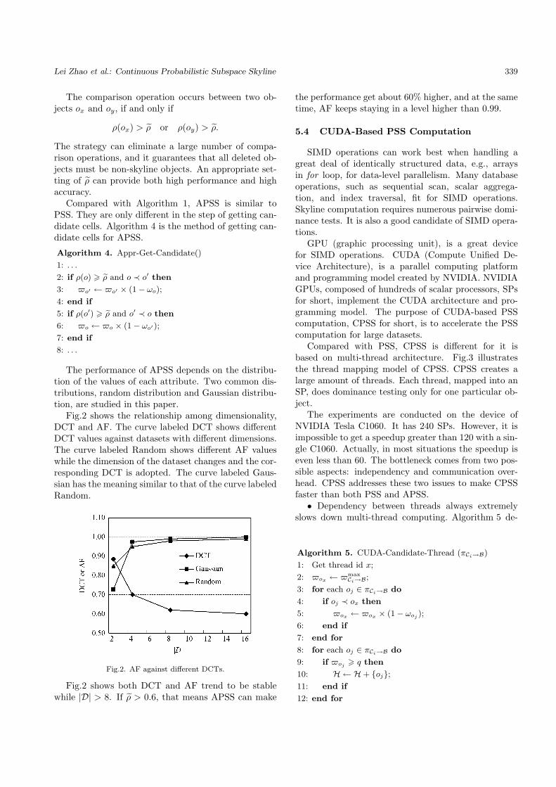
Fig.2 shows the relationship among dimensionality,DCT and AF. The curve labeled DCT shows differentDCT values against datasets with different dimensions.The curve labeled Random shows different AF valueswhile the dimension of the dataset changes and the cor-responding DCT is adopted. The curve labeled Gaus-sian has the meaning similar to that of the curve labeledRandom.

Fig.2. AF against different DCTs.

Fig.2 shows both DCT and AF trend to be stablewhile |D| > 8. If ρ > 0.6, that means APSS can make

the performance get about 60% higher, and at the sametime, AF keeps staying in a level higher than 0.99.

5.4 CUDA-Based PSS Computation

SIMD operations can work best when handling agreat deal of identically structured data, e.g., arraysin for loop, for data-level parallelism. Many databaseoperations, such as sequential scan, scalar aggrega-tion, and index traversal, fit for SIMD operations.Skyline computation requires numerous pairwise domi-nance tests. It is also a good candidate of SIMD opera-tions.

GPU (graphic processing unit), is a great devicefor SIMD operations. CUDA (Compute Unified De-vice Architecture), is a parallel computing platformand programming model created by NVIDIA. NVIDIAGPUs, composed of hundreds of scalar processors, SPsfor short, implement the CUDA architecture and pro-gramming model. The purpose of CUDA-based PSScomputation, CPSS for short, is to accelerate the PSScomputation for large datasets.

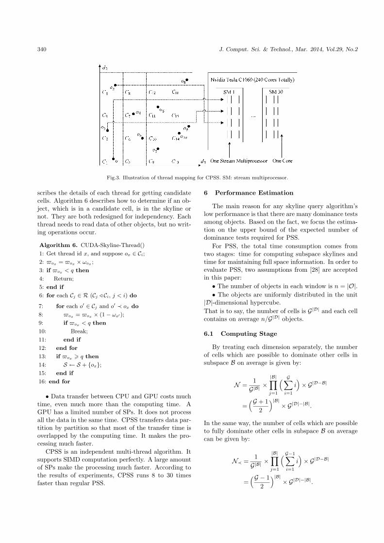
Compared with PSS, CPSS is different for it isbased on multi-thread architecture. Fig.3 illustratesthe thread mapping model of CPSS. CPSS creates alarge amount of threads. Each thread, mapped into anSP, does dominance testing only for one particular ob-ject.

The experiments are conducted on the device ofNVIDIA Tesla C1060. It has 240 SPs. However, it isimpossible to get a speedup greater than 120 with a sin-gle C1060. Actually, in most situations the speedup iseven less than 60. The bottleneck comes from two pos-sible aspects: independency and communication over-head. CPSS addresses these two issues to make CPSSfaster than both PSS and APSS.

• Dependency between threads always extremelyslows down multi-thread computing. Algorithm 5 de-

Algorithm 5. CUDA-Candidate-Thread (πCi→B)

1: Get thread id x;

2: $ox ← $maxCi→B;

3: for each oj ∈ πCi→B do

4: if oj ≺ ox then

5: $ox ← $ox × (1− ωoj );

6: end if

7: end for

8: for each oj ∈ πCi→B do

9: if $oj q then

10: H ← H+ {oj};11: end if

12: end for


Fig.3. Illustration of thread mapping for CPSS. SM: stream multiprocessor.

scribes the details of each thread for getting candidatecells. Algorithm 6 describes how to determine if an ob-ject, which is in a candidate cell, is in the skyline ornot. They are both redesigned for independency. Eachthread needs to read data of other objects, but no writ-ing operations occur.

Algorithm 6. CUDA-Skyline-Thread()

1: Get thread id x, and suppose ox ∈ Ci;

2: $ox = $ox × ωox ;

3: if $ox < q then

4: Return;

5: end if

6: for each Cj ∈ R (Cj / Ci, j < i) do

7: for each o′ ∈ Cj and o′ ≺ ox do

8: $ox = $ox × (1− ωo′);

9: if $ox < q then

10: Break;

11: end if

12: end for

13: if $ox q then

14: S ← S + {ox};15: end if

16: end for

• Data transfer between CPU and GPU costs muchtime, even much more than the computing time. AGPU has a limited number of SPs. It does not processall the data in the same time. CPSS transfers data par-tition by partition so that most of the transfer time isoverlapped by the computing time. It makes the pro-cessing much faster.

CPSS is an independent multi-thread algorithm. Itsupports SIMD computation perfectly. A large amountof SPs make the processing much faster. According tothe results of experiments, CPSS runs 8 to 30 timesfaster than regular PSS.

6 Performance Estimation

The main reason for any skyline query algorithm’slow performance is that there are many dominance testsamong objects. Based on the fact, we focus the estima-tion on the upper bound of the expected number ofdominance tests required for PSS.

For PSS, the total time consumption comes fromtwo stages: time for computing subspace skylines andtime for maintaining full space information. In order toevaluate PSS, two assumptions from [28] are acceptedin this paper:

• The number of objects in each window is n = |O|.• The objects are uniformly distributed in the unit

|D|-dimensional hypercube.That is to say, the number of cells is G|D| and each cellcontains on average n/G|D| objects.

6.1 Computing Stage

By treating each dimension separately, the numberof cells which are possible to dominate other cells insubspace B on average is given by:

N =1

G|B| ×|B|∏

j=1

( G∑

i=1

i)× G|D−B|

=(G + 1

2

)|B|× G|D|−|B|.

In the same way, the number of cells which are possibleto fully dominate other cells in subspace B on averagecan be given by:

N≺ =1

G|B| ×|B|∏

j=1

( G−1∑

i=1

i)× G|D−B|

=(G − 1

2

)|B|× G|D|−|B|.


Recall our algorithm that it is only necessary to com-pare object o with the objects contained in the cellsthat partially dominate C(o ∈ C) when computing theexact skyline probability of object o. So, we can getthe number of the cells which are possible to partiallydominate other cells in subspace B by subtracting N≺from N :

N/ =N −N≺

=((G + 1

2

)|B|−

(G − 12

)|B|)× G|D|−|B|.

It follows that the number of objects which are nece-ssary to be involved in dominance computations is

n′ =(N −N≺)× n

|G||D|

=((G + 1

2

)|B|−

(G − 12

)|B|)× G|D|

G|B| ×n

|G||D|

=((G + 1

2

)|B|−

(G − 12

)|B|)× n

|G||B| .

Let

f(G,B) =

((G + 12

)|B|−

(G − 12

)|B|)

|G||B| . (4)

Table 4 studies the values of f(G,B). Suppose, therange of n varies from 100K to 1 000K, then lg(n) variesfrom 5 to 6, and 1/ lg(n) falls into 0.166 7 to 0.200 0.Apparently, if G is large enough, then

f(G,B) ¿ 1lg(n)

.

It follows thatn′ ¿ n

lg(n).

Table 4. Values of f(G,B)

B = 2 B = 3 B = 4 B = 5

G = 10 0.100 0 0.075 3 0.050 5 0.031 9

G = 15 0.066 7 0.050 1 0.033 5 0.021 0

G = 20 0.017 4 0.013 7 0.009 7 0.006 4

It is not hard to see that the number of objectswhich are involved in dominance test is much lessthan the number of all objects in the active slide win-dow. Finally, the complexity of PSS computing stageis O(n/ lg(n)).

6.2 Maintaining Stage

In the maintaining stage of PSS, using the result of[29], the number of the objects which need to be checked

is

n′′ =((G + 1

2

)|D|+

(G − 12

)|D|)× n

G|D| .

According to (4), we have

n′′ = f(G,D).

By means of Table 4, we have

f(G,D) < f(G,B) ¿ 1lg(n)

.

Therefore, n′′ is also much less than n/ lg(n), and thecomplexity of PSS maintaining stage is O(n/ lg(n)).

7 Experiments

The evaluation of PSS uses a synthetic dataset gene-rated by a data generator tool according to three kindsof distributions[1], as well as a real e-business dataset.Table 5 lists the experimental setup.

Table 5. Experimental Setup

Setting

Language C++

Compiler GCC

Operating system CentOS Release 6.2

Processor Intel Xeon E5506

Memory 24GB

GPU NVIDIA Tesla C1060

7.1 Synthetic Data

The synthetic data space consists of n dimensionswhose domains have a range of [0, 10000.0) and the di-mensionality of n is in the range of 2 to 5. The occur-rence probability of each object takes a random valuebetween 0 and 1 (not include 1) and a count-based win-dow with size W between 100K and 500K objects. Ta-ble 6 summarizes the parameters of testing, along withtheir default values. The following elapsed time meansthe average response time of each query.

Table 6. Testing Parameters and Default Values

Parameter Range Default Value

W 100K∼500K 100K

D 2∼16 5.0

B 1∼5 3.0

q 0.1∼0.9 0.3

G 2∼10 8.0

For benchmarking, we make up the straightforwardmethod as the Naive algorithm, in which a heap is alsoused to keep the intermediate dominance results.


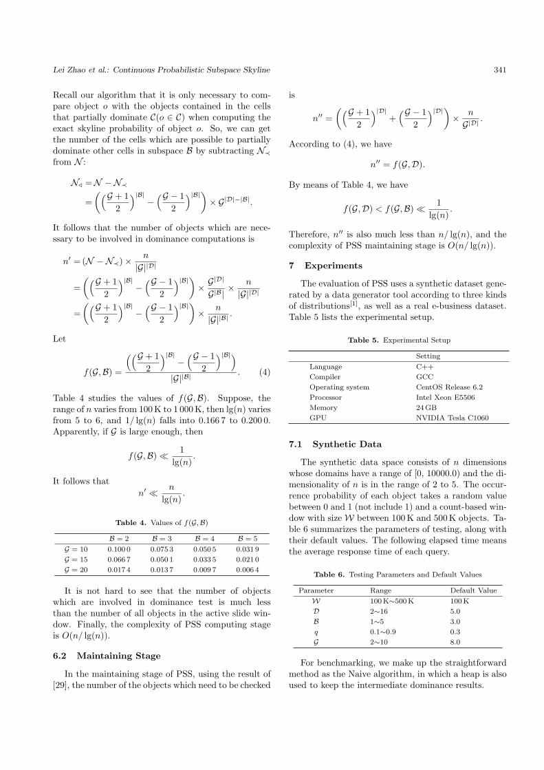
We first study the impact of the grid granularity onPSS for three kinds of data distribution, anti-correlated,independent, and correlated, named Anti., Indep., andCorr., respectively for short in Fig.4. Secondly, wecompare the efficiency of PSS algorithm against proba-bilistic threshold, query dimensions and the size of slid-ing window with Naive algorithm.

We test the impact of the grid granularity on PSSand try to find an appropriate G. Fig.4 illustrates thatthe dense granularity may have a short time-consuming,but it also leads to higher space consumption. For fair-ness, we take 8 for the best value of G because this valueprovides the best performance with reasonable spacerequirements. Moreover, the space cost of PSS for thethree kinds of distributions are almost the same, thusthere is only one single curve in Fig.4(b).

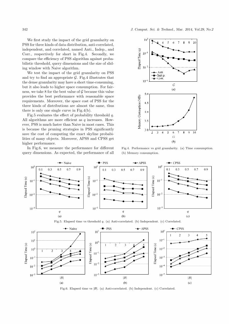
Fig.5 evaluates the effect of probability threshold q.All algorithms are more efficient as q increases. How-ever, PSS is much faster than Naive in most cases. Thisis because the pruning strategies in PSS significantlysave the cost of computing the exact skyline probabi-lities of many objects. Moreover, APSS and CPSS gethigher performance.

In Fig.6, we measure the performance for differentquery dimensions. As expected, the performance of all

Fig.4. Performance vs grid granularity. (a) Time consumption.

(b) Memory consumption.

Fig.5. Elapsed time vs threshold q. (a) Anti-correlated. (b) Independent. (c) Correlated.

Fig.6. Elapsed time vs |B|. (a) Anti-correlated. (b) Independent. (c) Correlated.


Fig.7. Elapsed time vs size of window. (a) Anti-correlated. (b) Independent. (c) Correlated.

algorithms degrades while |B| is getting higher. Ini-tially, the costs of Naive and PSS are similar for anti-correlated and independent data, but they becomemuch different while |B| is getting higher.

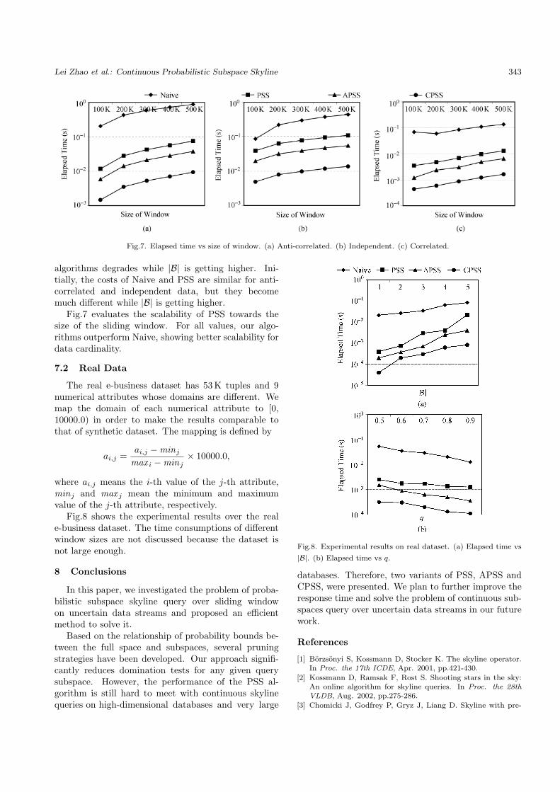
Fig.7 evaluates the scalability of PSS towards thesize of the sliding window. For all values, our algo-rithms outperform Naive, showing better scalability fordata cardinality.

7.2 Real Data

The real e-business dataset has 53K tuples and 9numerical attributes whose domains are different. Wemap the domain of each numerical attribute to [0,10000.0) in order to make the results comparable tothat of synthetic dataset. The mapping is defined by

ai,j =ai,j −minj

max i −minj× 10000.0,

where ai,j means the i-th value of the j-th attribute,minj and max j mean the minimum and maximumvalue of the j-th attribute, respectively.

Fig.8 shows the experimental results over the reale-business dataset. The time consumptions of differentwindow sizes are not discussed because the dataset isnot large enough.

8 Conclusions

In this paper, we investigated the problem of proba-bilistic subspace skyline query over sliding windowon uncertain data streams and proposed an efficientmethod to solve it.

Based on the relationship of probability bounds be-tween the full space and subspaces, several pruningstrategies have been developed. Our approach signifi-cantly reduces domination tests for any given querysubspace. However, the performance of the PSS al-gorithm is still hard to meet with continuous skylinequeries on high-dimensional databases and very large

Fig.8. Experimental results on real dataset. (a) Elapsed time vs

|B|. (b) Elapsed time vs q.

databases. Therefore, two variants of PSS, APSS andCPSS, were presented. We plan to further improve theresponse time and solve the problem of continuous sub-spaces query over uncertain data streams in our futurework.

References

[1] Borzsonyi S, Kossmann D, Stocker K. The skyline operator.In Proc. the 17th ICDE, Apr. 2001, pp.421-430.

[2] Kossmann D, Ramsak F, Rost S. Shooting stars in the sky:An online algorithm for skyline queries. In Proc. the 28thVLDB, Aug. 2002, pp.275-286.

[3] Chomicki J, Godfrey P, Gryz J, Liang D. Skyline with pre-


sorting. In Proc. the 19th ICDE, Mar. 2003, pp.717-719.[4] Tao Y, Papadias D. Maintaining sliding window skylines on

data streams. IEEE Trans. Knowl. Data Eng., 2006, 18(2):377-391.

[5] Zhang W, Lin X, Zhang Y, Wang W, Yu J X. Probabilisticskyline operator over sliding windows. In Proc. the 25thICDE, Mar. 29-Apr. 2, 2009, pp.1060-1071.

[6] Tan K L, Eng P K, Ooi B C. Efficient progressive skyline com-putation. In Proc. the 27th VLDB, Sept. 2001, pp.301-310.

[7] Godfrey P, Shipley R, Gryz J. Maximal vector computationin large datasets. In Proc. the 31st VLDB, Aug. 30-Sept. 2,2005, pp.229-240.

[8] Papadias D, Tao Y, Fu G et al. An optimal and progressivealgorithm for skyline queries. In Proc. the 22nd SIGMOD,Jun. 2003, pp.467-478.

[9] Lee K C K, Zheng B, Li H, Lee W C. Approaching the skylinein Z order. In Proc. the 33rd VLDB, Sept. 2007, pp.279-290.

[10] Lee J, Hwang S. BSkyTree: Scalable skyline computation us-ing a balanced pivot selection. In Proc. the 13th EDBT, Mar.2010, pp.195-206.

[11] Zhang S, Mamoulis N, Cheung D W. Scalable skyline com-putation using object-based space partitioning. In Proc. the28th SIGMOD, Jun. 29-July 2, 2009, pp.483-494.

[12] Lin X, Zhang Y, Zhang W, Cheema M A. Stochastic skylineoperator. In Proc. the 27th ICDE, Apr. 2011, pp.721-732.

[13] Kohler H, Yang J, Zhou X. Efficient parallel skyline processingusing hyperplane projections. In Proc. the 30th SIGMOD,Jun. 2011, pp.85-96.

[14] Cho S R, Lee J, Hwang S W. Vskyline: Vectorization for effi-cient skyline computation. In Proc. the 29th SIGMOD, Jun.2010, pp.19-26.

[15] Kontaki M, Papadopoulos A N, Manolopoulos Y. Continu-ous top-k dominating queries in subspaces. In Proc. the 2008Panhellenic Conference on Informatics, Aug. 2008, pp.31-35.

[16] Yiu M L, Mamoulis N. Multi-dimensional top-k dominatingqueries. VLDB J., 2009, 18(3): 695-718.

[17] Lian X, Chen L. Monochromatic and bichromatic reverse sky-line search over uncertain databases. In Proc. the 2008 SIG-MOD, Jun. 2008, pp.213-226.

[18] Zhang W, Lin X, Zhang Y, Pei J, Wang W. Threshold-basedprobabilistic top-k dominating queries. VLDB J., 2010, 19(2):283-305.

[19] Lin X, Yuan Y, Wang W, Lu H. Stabbing the sky: Efficientskyline computation over sliding windows. In Proc. the 21stICDE, Apr. 2005, pp.502-513.

[20] Morse M D, Patel J M, Grosky W I. Efficient continuous sky-line computation. In Proc. the 22nd ICDE, Apr. 2006, p.108.

[21] Pei J, Jin W, Ester M, Tao Y. Catching the best views ofskyline: A semantic approach based on decisive subspaces. InProc. the 31st VLDB, Aug. 30-Sept. 2, 2005, pp.253-264.

[22] Yuan Y, Lin X, Liu Q, Wang W, Yu J X , Zhang Q. Efficientcomputation of the skyline cube. In Proc. the 31st VLDB,Oct. 2005, pp.241-252.

[23] Tao Y, Xiao X , Pei J. SUBSKY: Efficient computation ofskylines in subspaces. In Proc. the 22nd ICDE, Apr. 2006,p.65.

[24] Pei J, Fu A W, Lin X, Wang H. Computing compressed multi-dimensional skyline cubes efficiently. In Proc. the 23rd ICDE,Apr. 2007, pp.96-105.

[25] Raıssi C, Pei J, Kister T. Computing closed skycubes.PVLDB, 2010, 3(1): 838-847.

[26] Pei J, Jiang B, Lin X, Yuan Y. Probabilistic skylines on un-certain data. In Proc. the 33rd VLDB, Sept. 2007, pp.15-26.

[27] Atallah M J, Qi Y. Computing all skyline probabilities for un-certain data. In Proc. the 28th PODS, Jun. 29-July 2, 2009,pp.279-287.

[28] Mouratidis K, Bakiras S, Papadias D. Continuous monitor-ing of top-k queries over sliding windows. In Proc. the 2006SIGMOD, Jun. 2006, pp.635-646.

[29] Kontaki M, Papadopoulos A N, Manolopoulos Y. Continuoustop-k dominating queries. IEEE Trans. Knowl. Data Eng.,2012, 24(5): 840-853.

Lei Zhao received the Ph.D. de-gree in computer science from Soo-chow University, China, in 2006.He has been a faculty member ofthe School of Computer Science andTechnology of Soochow Universitysince 1998. He is now an associateprofessor of the Department of Net-work Engineering. His research in-terests include distributed data pro-

cessing, data mining, parallel and distributed computing,etc.

Yan-Yan Yang received theMaster degree in computer sciencefrom Soochow University, Suzhou, in2012. She has been an engineerof storage testing at IBM Corpora-tion since 2012. Her research inter-ests include distributed data process-ing, database query optimizing, datamining, etc.

Xiaofang Zhou is a professor ofcomputer science at the University ofQueensland. He received his B.Sc.and M.Sc. degrees in computer sci-ence from Nanjing University, China,and Ph.D. degree in computer sci-ence from the University of Queens-land, Australia. His research focusis to find effective and efficient solu-tions for managing, integrating and

analyzing very large amount of complex data for business,scientific, and personal applications. He has been workingin the area of spatial and multimedia databases, data qual-ity management, in-memory databases, high-performancequery processing, Web information systems, data miningand bioinformatics.

continuous probabilistic subspace skyline query processing using grid projections

Documents