copyright © 2011 pearson education, inc. regression diagnostics chapter 22
TRANSCRIPT
Copyright © 2011 Pearson Education, Inc.
Regression Diagnostics
Chapter 22
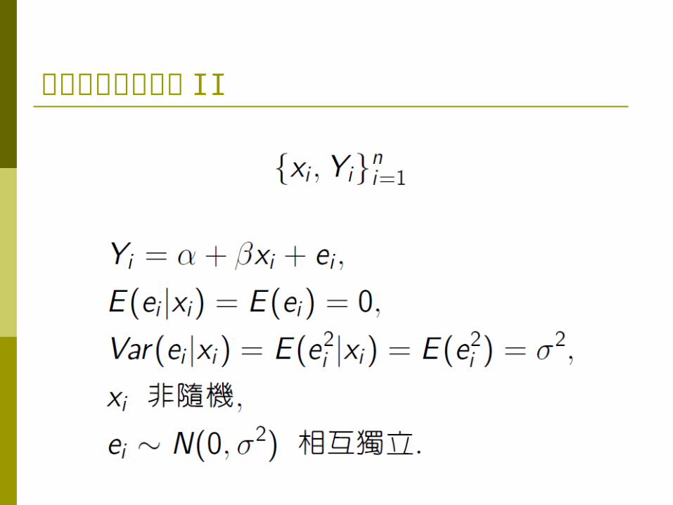
古典常態迴歸模型 II
22.1 Problem 1: Changing Variation
Although regression analysis allows the use of prices of different size homes to estimate the home of a specific size, prices tend to be more variable for larger homes. How does this affect the SRM?
Consider how to recognize and fix three potential problems affecting regression models: changing variation in the data, outliers, and dependence among observations
Copyright © 2011 Pearson Education, Inc.
3 of 48
22.1 Problem 1: Changing Variation
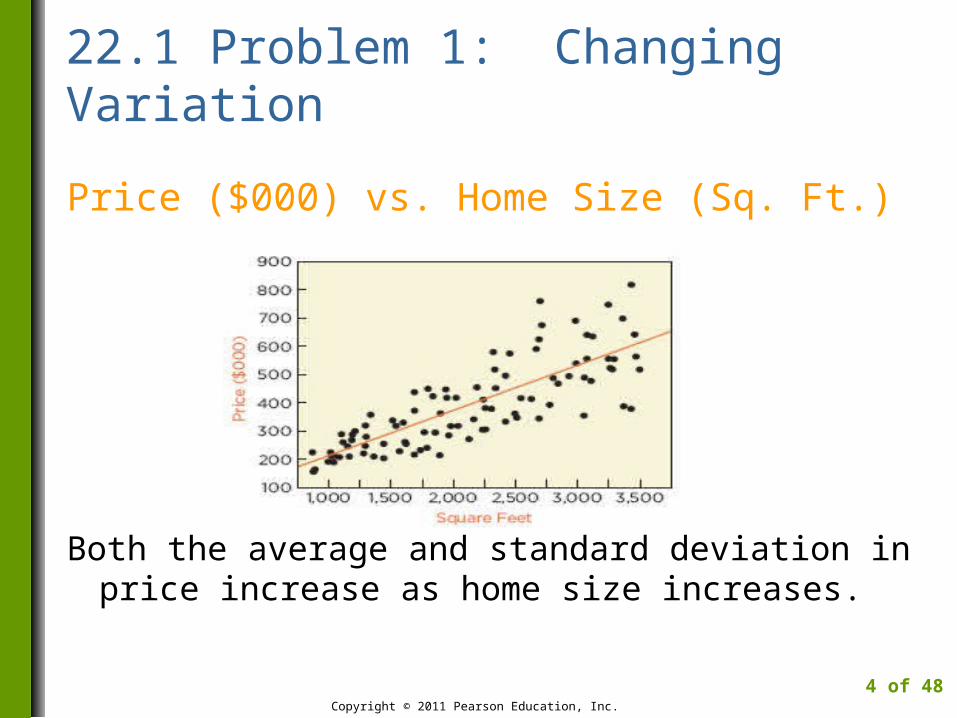
Price ($000) vs. Home Size (Sq. Ft.)
Both the average and standard deviation in price increase as home size increases.
Copyright © 2011 Pearson Education, Inc.
4 of 48
22.1 Problem 1: Changing Variation
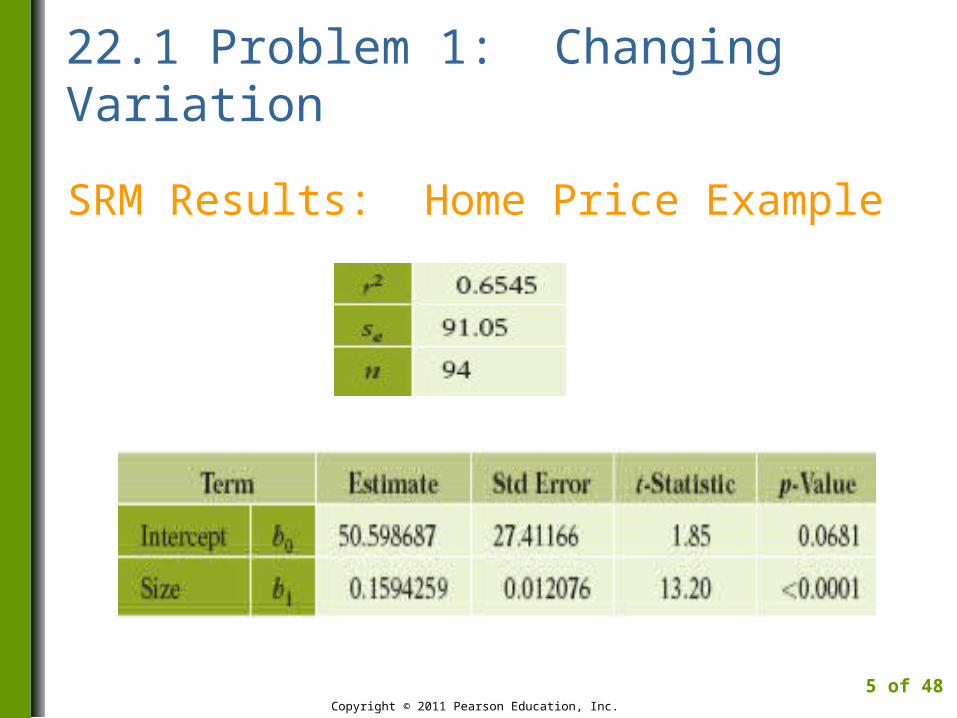
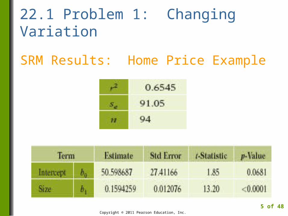
SRM Results: Home Price Example
Copyright © 2011 Pearson Education, Inc.
5 of 48
22.1 Problem 1: Changing Variation
Fixed Costs, Marginal Costs, and Variable Costs
The estimated intercept (50.598687) can be interpreted as the fixed cost of a home.
The 95% confidence interval for the intercept (after rounding) is -$4,000 to $105,000.
Since it includes zero, this interval is not a precise estimate of fixed costs.
Copyright © 2011 Pearson Education, Inc.
6 of 48
22.1 Problem 1: Changing Variation
Fixed Costs, Marginal Costs, and Variable Costs
The slope (0.1594259) estimates the marginal cost of an additional square foot of space.
The 95% confidence interval for the slope (after rounding) is $135,000 to $183,500.
It can be interpreted as the average difference in home price associated with 1,000 square feet.
Copyright © 2011 Pearson Education, Inc.
7 of 48
22.1 Problem 1: Changing Variation
Detecting Differences in Variation
Based on the scatterplot, the association between home price and size appears linear.
Little concern about lurking variables since the sample of homes is from the same neighborhood.
Similar variances condition is not satisfied.
Copyright © 2011 Pearson Education, Inc.
8 of 48
22.1 Problem 1: Changing Variation
Detecting Differences in Variation
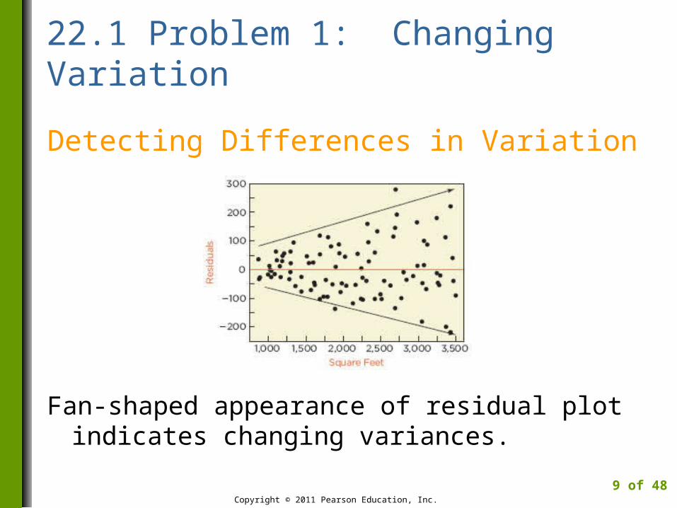
Fan-shaped appearance of residual plot indicates changing variances.
Copyright © 2011 Pearson Education, Inc.
9 of 48
22.1 Problem 1: Changing Variation
Detecting Differences in Variation
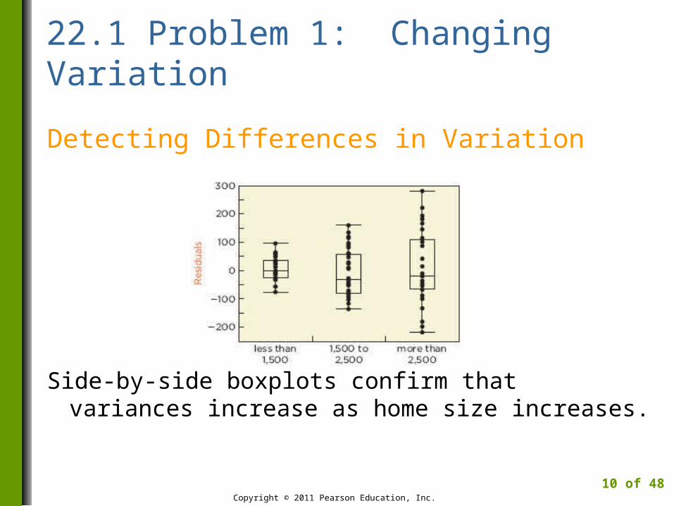
Side-by-side boxplots confirm that variances increase as home size increases.
Copyright © 2011 Pearson Education, Inc.
10 of 48
22.1 Problem 1: Changing Variation
Detecting Differences in Variation
Heteroscedastic: errors that have different amounts of variation.
Homoscedastic: errors having equal amounts of variation.
Copyright © 2011 Pearson Education, Inc.
11 of 48
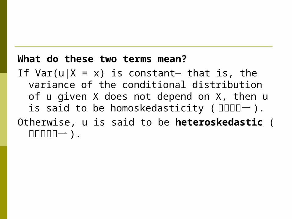
What do these two terms mean?If Var(u|X = x) is constant— that is, the variance of
the conditional distribution of u given X does not depend on X, then u is said to be homoskedasticity (變異數齊一 ).
Otherwise, u is said to be heteroskedastic (變異數不齊一 ).
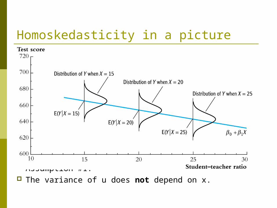
Homoskedasticity in a picture
E(u|X = x) = 0, u satisfies Least Squares Assumption #1.
The variance of u does not depend on x.
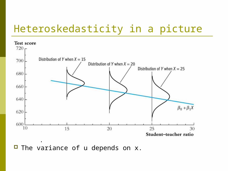
Heteroskedasticity in a picture
E(u|X = x) = 0, u satisfies Least Squares Assumption #1.
The variance of u depends on x.
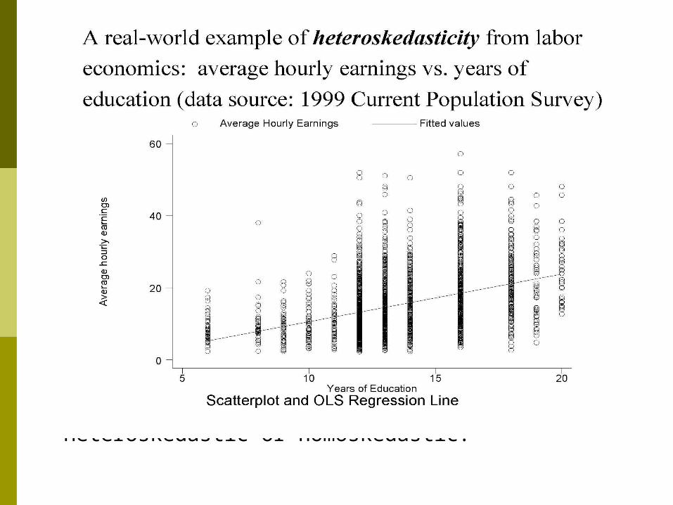
Heteroskedastic or homoskedastic?
22.1 Problem 1: Changing Variation
Consequences of Different Variation
Prediction intervals are too narrow or too wide.
Confidence intervals for the slope and intercept are not reliable.
Hypothesis tests regarding β0 and β1 are not reliable.
Copyright © 2011 Pearson Education, Inc.
12 of 48
22.1 Problem 1: Changing Variation
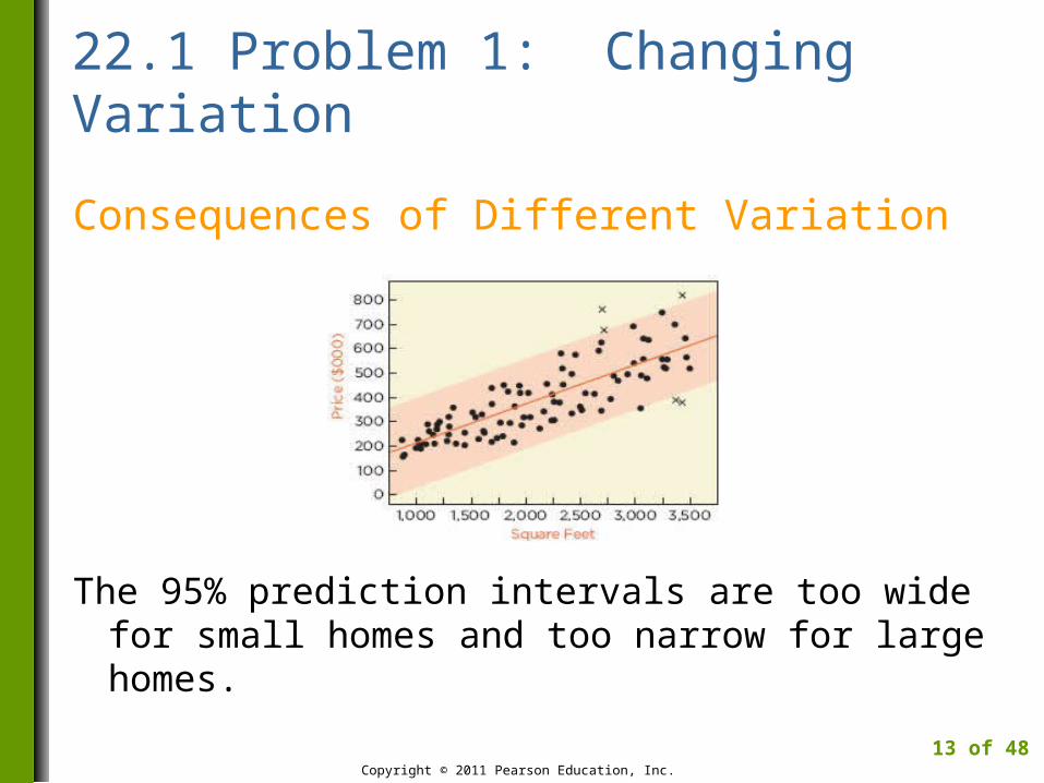
Consequences of Different Variation
The 95% prediction intervals are too wide for small homes and too narrow for large homes.
Copyright © 2011 Pearson Education, Inc.
13 of 48
22.1 Problem 1: Changing Variation
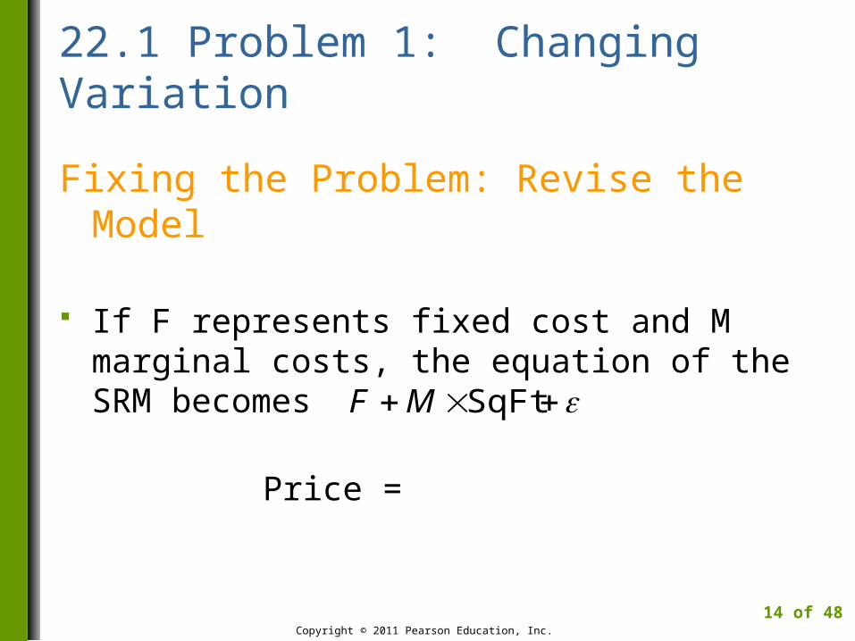
Fixing the Problem: Revise the Model
If F represents fixed cost and M marginal costs, the equation of the SRM becomes
Price =
Copyright © 2011 Pearson Education, Inc.
14 of 48
SqFtMF
22.1 Problem 1: Changing Variation
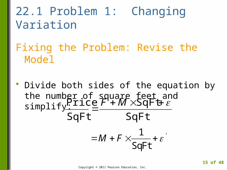
Fixing the Problem: Revise the Model
Divide both sides of the equation by the number of square feet and simplify:
Copyright © 2011 Pearson Education, Inc.
15 of 48
SqFt
SqFt
SqFt
Price
MF
'1
SqFtM F
22.1 Problem 1: Changing Variation
Fixing the Problem: Revise the Model
The response variable becomes price per square foot and the explanatory variable becomes the reciprocal of the number of square feet.
The marginal cost M is the intercept and the slope is F, the fixed cost.
The residuals have similar variances.
Copyright © 2011 Pearson Education, Inc.
16 of 48
22.1 Problem 1: Changing Variation
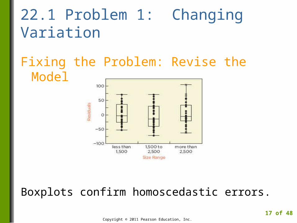
Fixing the Problem: Revise the Model
Boxplots confirm homoscedastic errors.
Copyright © 2011 Pearson Education, Inc.
17 of 48
4M Example 22.1: ESTIMATING HOME PRICES
Motivation
A company is relocating several managers to the Seattle area. For budgeting purposes, they would like a break down of home prices into fixed and variable costs to better prepare for negotiations with realtors.
Copyright © 2011 Pearson Education, Inc.
18 of 48
4M Example 22.1: ESTIMATING HOME PRICES
Method
Data consists of a sample of 94 homes for sale in Seattle. The explanatory variable is the reciprocal of home size and the response is price per square foot. The scatterplot shows a linear association and there are no obvious lurking variables.
Copyright © 2011 Pearson Education, Inc.
19 of 48
4M Example 22.1: ESTIMATING HOME PRICES
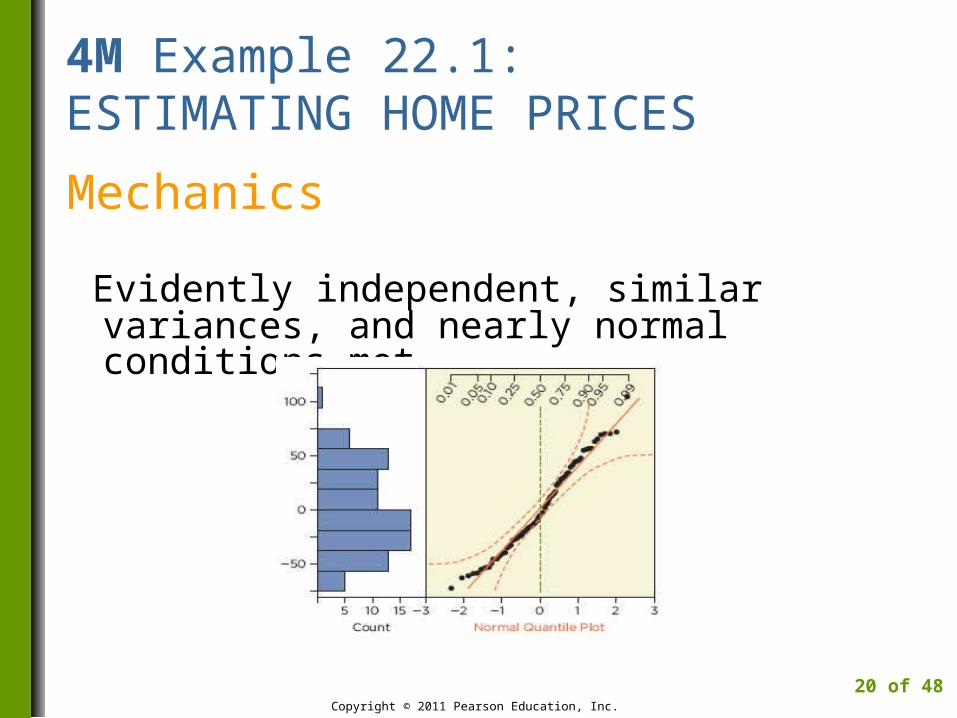
Mechanics
Evidently independent, similar variances, and nearly normal conditions met.
Copyright © 2011 Pearson Education, Inc.
20 of 48
4M Example 22.1: ESTIMATING HOME PRICES
Mechanics
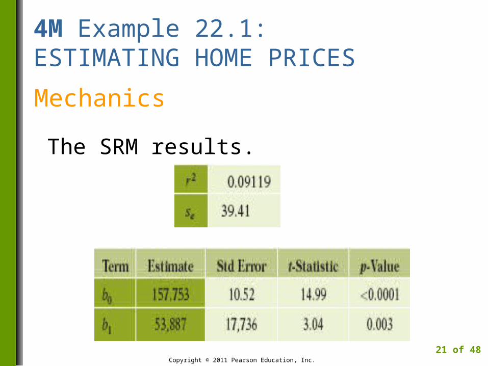
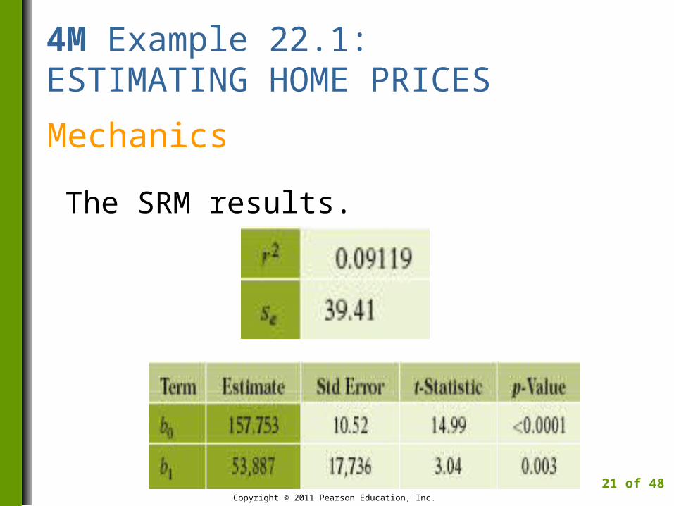
The SRM results.
Copyright © 2011 Pearson Education, Inc.
21 of 48
4M Example 22.1: ESTIMATING HOME PRICES
Mechanics
The fitted equation is
Estimated $/SqFt = 157.753 + 53,887/SqFt.
The 95% confidence interval for the intercept is [136.8182 to 178.6878] and the 95% confidence interval for the slope is [18,592.36 to 89,181.64].
Copyright © 2011 Pearson Education, Inc.
22 of 48
4M Example 22.1: ESTIMATING HOME PRICES
Message
Prices for homes in this Seattle neighborhood run about $140 to $180 per square foot, on average. Average fixed costs associated with the purchase are in the range $19,000 to $89,000, with 95% confidence.
Copyright © 2011 Pearson Education, Inc.
23 of 48
22.1 Problem 1: Changing Variation
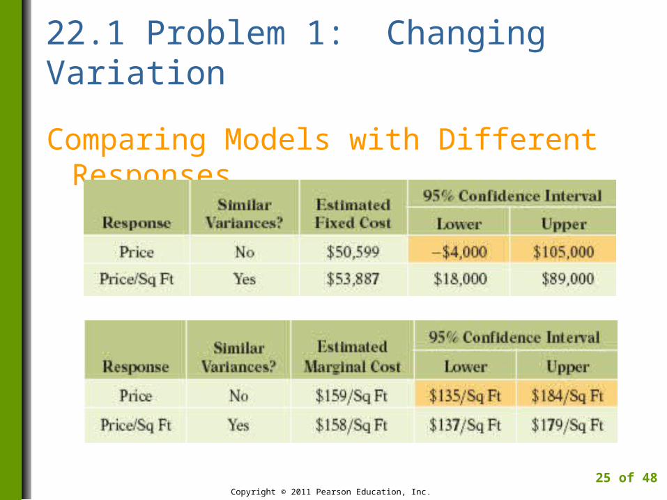
Comparing Models with Different Responses
Even though the revised model has a smaller r2,
It provides more reliable and narrower confidence intervals for fixed and variable costs; and
It provides more sensible prediction intervals.
Copyright © 2011 Pearson Education, Inc.
24 of 48
22.1 Problem 1: Changing Variation
SRM Results: Home Price Example
Copyright © 2011 Pearson Education, Inc.
5 of 48
4M Example 22.1: ESTIMATING HOME PRICES
Mechanics
The SRM results.
Copyright © 2011 Pearson Education, Inc.
21 of 48
22.1 Problem 1: Changing Variation
Comparing Models with Different Responses
Copyright © 2011 Pearson Education, Inc.
25 of 48
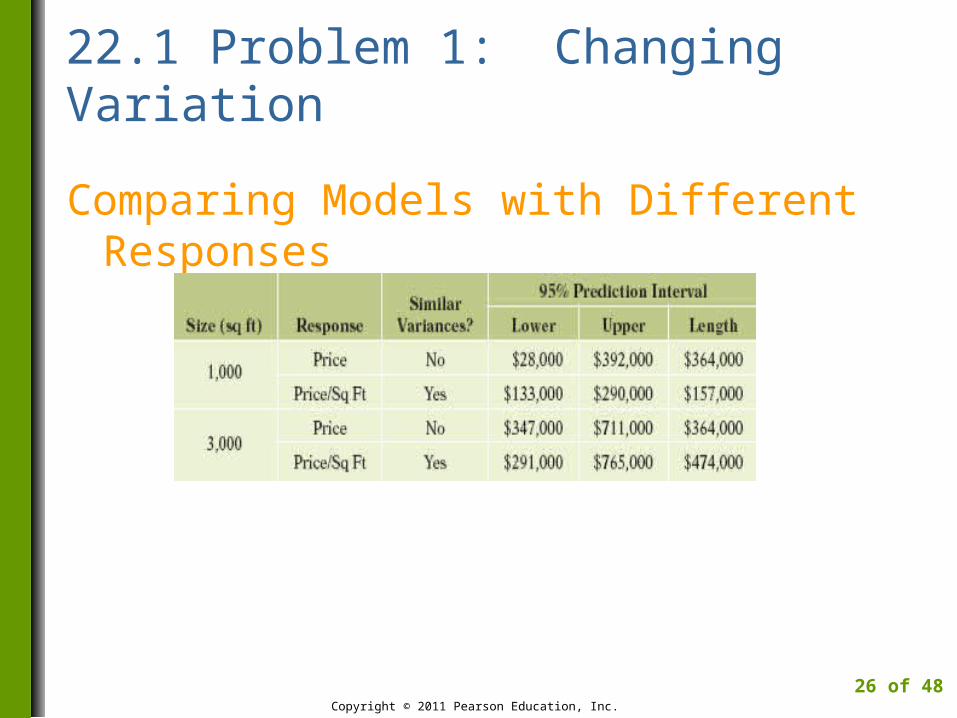
22.1 Problem 1: Changing Variation
Comparing Models with Different Responses
Copyright © 2011 Pearson Education, Inc.
26 of 48

22.2 Problem 2: Leveraged Outliers
Consider a Contractor’s Bid on a Project
A contractor is bidding on a project to construct an 875 square-foot addition to a home.
If he bids too low, he loses money on the project.
If he bids too high, he does not get the job.
Copyright © 2011 Pearson Education, Inc.
27 of 48
22.2 Problem 2: Leveraged Outliers
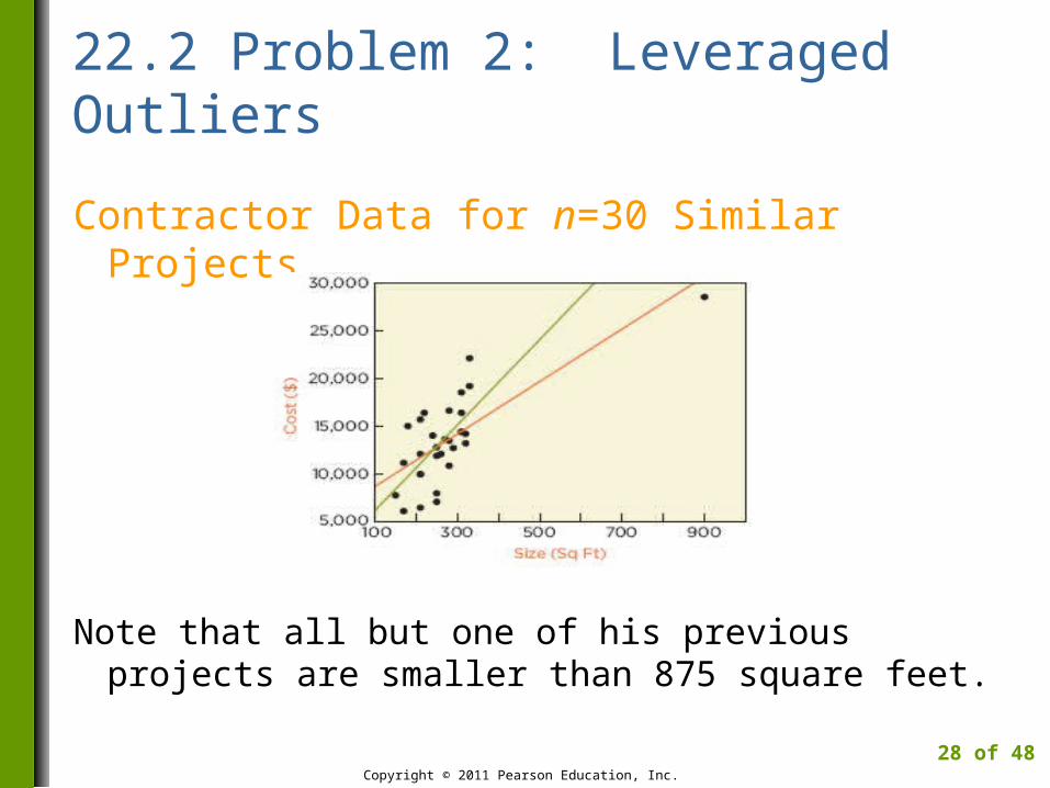
Contractor Data for n=30 Similar Projects
Note that all but one of his previous projects are smaller than 875 square feet.
Copyright © 2011 Pearson Education, Inc.
28 of 48
22.2 Problem 2: Leveraged Outliers
Contractor Example
His one project at 900 square feet is an outlier.
It is also a leveraged observation as it pulls the regression line in its direction.
Leveraged: an observation in regression that has a small or large value of the explanatory variable.
Copyright © 2011 Pearson Education, Inc.
29 of 48
22.2 Problem 2: Leveraged Outliers
Consequences of an Outlier
To see the consequences of an outlier, fit the least squares regression line both with and without it.
Use the standard errors obtained without including the outlier to compare estimates.
Copyright © 2011 Pearson Education, Inc.
30 of 48
22.2 Problem 2: Leveraged Outliers
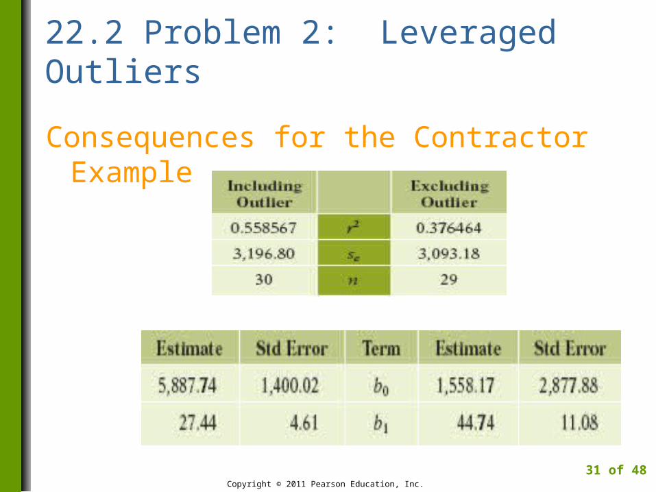
Consequences for the Contractor Example
Copyright © 2011 Pearson Education, Inc.
31 of 48
22.2 Problem 2: Leveraged Outliers
Consequences for the Contractor Example
Including the outlier shifts the estimated fixed cost up by about 1.5 standard errors.
Including the outlier shifts the estimated marginal cost down by about 1.56 standard errors.
Copyright © 2011 Pearson Education, Inc.
32 of 48
22.2 Problem 2: Leveraged Outliers
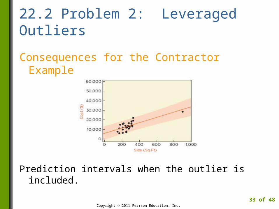
Consequences for the Contractor Example
Prediction intervals when the outlier is included.
Copyright © 2011 Pearson Education, Inc.
33 of 48
22.2 Problem 2: Leveraged Outliers
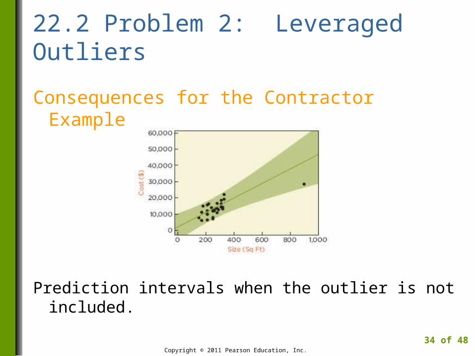
Consequences for the Contractor Example
Prediction intervals when the outlier is not included.
Copyright © 2011 Pearson Education, Inc.
34 of 48
22.2 Problem 2: Leveraged Outliers
Fixing the Problem: More Information
If the outlier describes what is expected the next time under the same conditions, then it should be included.
In the contractor example, more information is needed to decide whether to include or exclude the outlier.
Copyright © 2011 Pearson Education, Inc.
35 of 48
22.3 Problem 3: Dependent Errors and Time Series
Detecting Dependence
With time series data, plot residuals versus time to look for a pattern indicating dependence in the errors.
Use the Durbin-Watson statistic to test for correlation between adjacent residuals (known as autocorrelation).
Copyright © 2011 Pearson Education, Inc.
36 of 48
22.3 Problem 3: Dependent Errors and Time Series
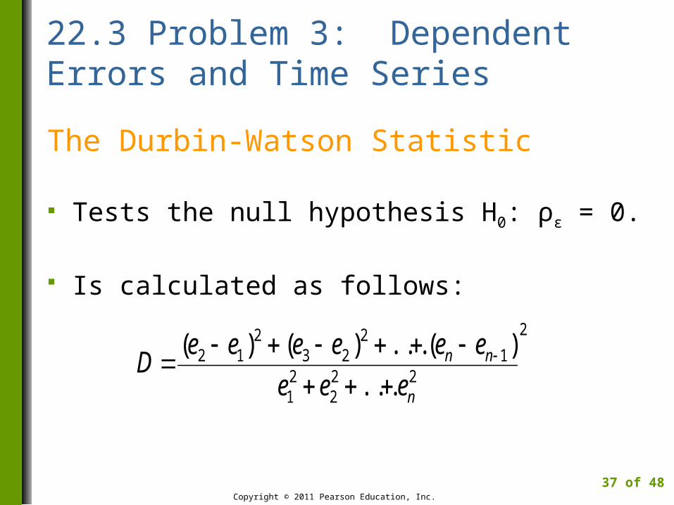
The Durbin-Watson Statistic
Tests the null hypothesis H0: ρε = 0.
Is calculated as follows:
Copyright © 2011 Pearson Education, Inc.
37 of 48
2
222
21
12
232
12
...
)(...)()(
n
nn
eee
eeeeeeD
22.3 Problem 3: Dependent Errors and Time Series
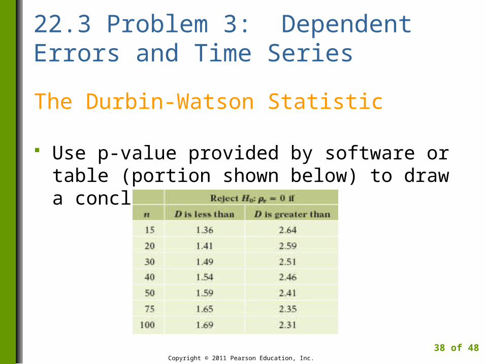
The Durbin-Watson Statistic
Use p-value provided by software or table (portion shown below) to draw a conclusion.
Copyright © 2011 Pearson Education, Inc.
38 of 48
22.3 Problem 3: Dependent Errors and Time Series
Consequences of Dependence
If there is positive autocorrelation in the errors, the estimated standard errors are too small.
The estimated slope and intercept are less precise than suggested by the output.
Best remedy is to incorporate the dependence into the regression model.
Copyright © 2011 Pearson Education, Inc.
39 of 48
4M Example 22.2: CELL PHONE SUBSCRIBERS
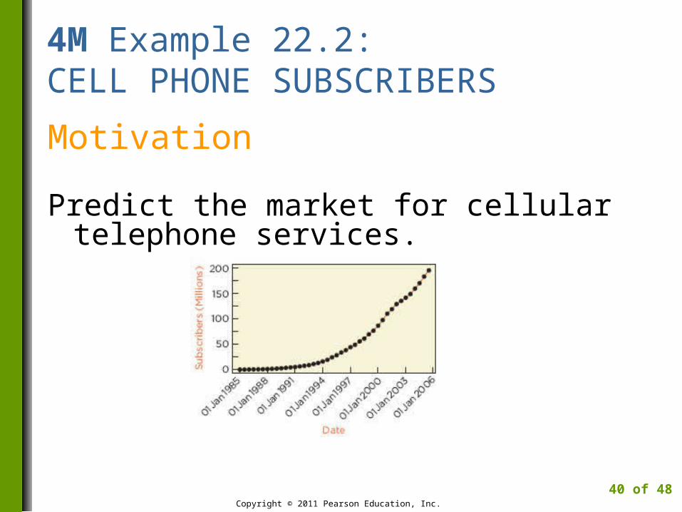
Motivation
Predict the market for cellular telephone services.
Copyright © 2011 Pearson Education, Inc.
40 of 48
4M Example 22.2: CELL PHONE SUBSCRIBERS
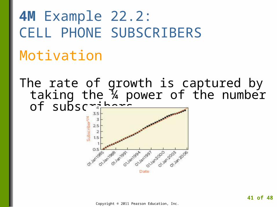
Motivation
The rate of growth is captured by taking the ¼ power of the number of subscribers.
Copyright © 2011 Pearson Education, Inc.
41 of 48
4M Example 22.2: CELL PHONE SUBSCRIBERS
Method
Use simple regression to predict the future number of subscribers. The quarter power of the number of subscribers, in millions, is the response. The explanatory variable is time. The scatterplot shows a linear association. Other lurking variables may be present, however, such as technology and marketing.
Copyright © 2011 Pearson Education, Inc.
42 of 48
4M Example 22.2: CELL PHONE SUBSCRIBERS
Mechanics
The least squares equation is
Estimated Subscribers1/4 = -317.4 + 0.16 Date
Copyright © 2011 Pearson Education, Inc.
43 of 48
4M Example 22.2: CELL PHONE SUBSCRIBERS
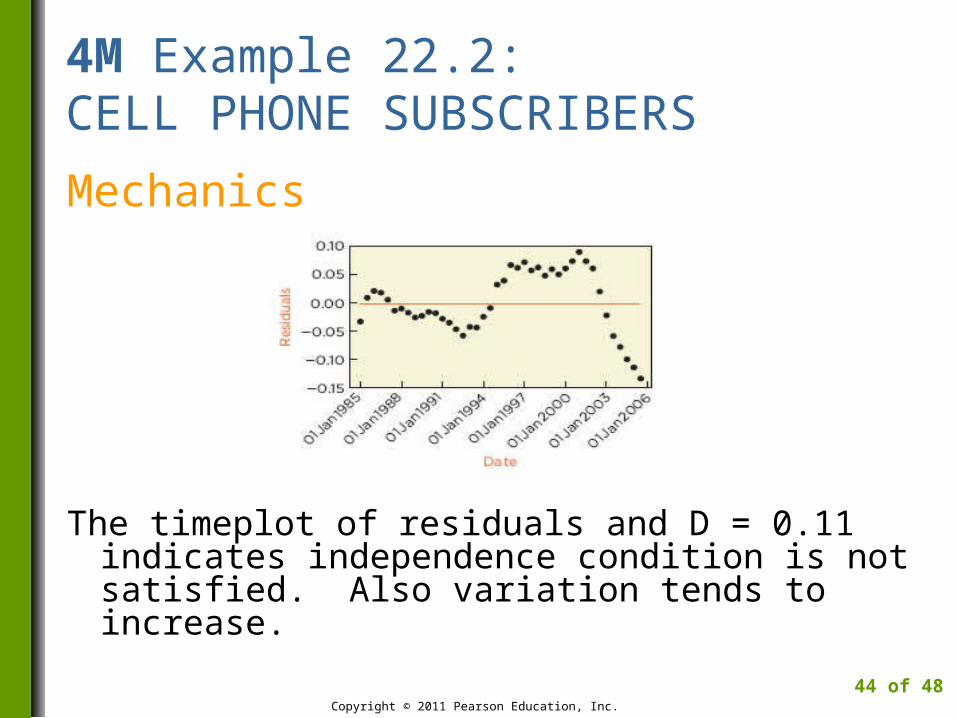
Mechanics
The timeplot of residuals and D = 0.11 indicates independence condition is not satisfied. Also variation tends to increase.
Copyright © 2011 Pearson Education, Inc.
44 of 48
4M Example 22.2: CELL PHONE SUBSCRIBERS
Message
Using a novel transformation, the historical trend can be summarized as
Estimated Subscribers1/4 = -317.4 + 0.16 Date.
However, since the conditions for SRM are not satisfied, we cannot quantify the uncertainty for predictions.
Copyright © 2011 Pearson Education, Inc.
45 of 48
Best Practices
Make sure that your model makes sense.
Plan to change your model if it does not match the data.
Report the presence of and how you handle any outliers.
Copyright © 2011 Pearson Education, Inc.
46 of 48
Pitfalls
Do not rely on summary statistics like r2 to pick the best model.
Don’t compare r2 between regression models unless the response is the same.
Do not check for normality until you get the right equation.
Copyright © 2011 Pearson Education, Inc.
47 of 48
Pitfalls (Continued)
Don’t think that your data are independent if the Durbin-Watson statistic is close to 2.
Never forget to look at plots of the data and model.
Copyright © 2011 Pearson Education, Inc.
48 of 48