creep of the austenitic steel aisi 316 l(n)
TRANSCRIPT
Forschungszentrum Karlsruhe in der Helmholtz-Gemeinschaft Wissenschaftliche Berichte FZKA 7065
Creep of the Austenitic Steel AISI 316 L(N) Experiments and Models M. Rieth, A. Falkenstein, P. Graf, S. Heger, U. Jäntsch, M. Klimiankou, E. Materna-Morris, H. Zimmermann Institut für Materialforschung Programm Kernfusion November 2004
Forschungszentrum Karlsruhe
in der Helmholtz-Gemeinschaft
Wissenschaftliche Berichte
FZKA 7065
Creep of the austenitic steel AISI 316 L(N)
– Experiments and Models –
M. Rieth, A. Falkenstein, P. Graf, S. Heger, U. Jäntsch, M. Klimiankou, E. Materna-Morris, H. Zimmermann
Institut für Materialforschung
Programm Kernfusion
Forschungszentrum Karlsruhe GmbH, Karlsruhe
2004
Impressum der Print-Ausgabe:
Als Manuskript gedruckt Für diesen Bericht behalten wir uns alle Rechte vor
Forschungszentrum Karlsruhe GmbH
Postfach 3640, 76021 Karlsruhe
Mitglied der Hermann von Helmholtz-Gemeinschaft Deutscher Forschungszentren (HGF)
ISSN 0947-8620
urn:nbn:de:0005-070657

i
ABSTRACT
This report provides a general review on deformation mechanisms relevant for metallic mate-rials. Different mechanisms are described by rate equations which are derived and discussed in detail. For the example of an austenitic 17Cr12Ni2Mo steel (AISI 316 L(N) or DIN 1.4909) these equations are applied to experimental creep data from own investigations at IMF-I (es-pecially long-term creep tests with creep times of up to 10 years) and from NRIM, Japan. Step-by-step a steady-state creep model is set up that is able to predict creep behaviour in a wide temperature and stress range. Due to the small number of adjustable parameters it may also be easily adapted to other materials. Since austenitic stainless steels are well known for their problematic aging behaviour at elevated temperatures, microstructure and precipitation formation as well as their impact on creep are outlined above all.
ii
Kriechverhalten des austenitischen Stahls AISI 316 L(N)
– Experimente und Modelle –
ZUSAMMENFASSUNG Der vorliegende Bericht beinhaltet eine allgemeine Übersicht über Verformungsmechanis-men, die bei metallischen Werkstoffen auftreten können. Dabei werden Gleichungen für die unterschiedlichen Mechanismen hergeleitet und ausführlich diskutiert. Am Beispiel eines austenitischen 17Cr12Ni2Mo-Stahls (AISI 316 L(N) oder DIN 1.4909) findet dann die An-wendung dieser Gleichungen auf experimentelle Kriechdaten aus eigenen Untersuchungen im IMF-I (insbesondere Langzeitkriechuntersuchungen mit Versuchszeiten von bis zu 10 Jahren) und von NRIM, Japan statt. Dadurch wird schrittweise ein Modell für das stationäre Kriechen aufgestellt, das das Kriechverhalten in einem weiten Temperatur- und Spannungs-bereich vorhersagen kann. Auf Grund der wenigen anzupassenden Parameter kann es auch leicht auf andere Werkstoffe angewandt werden. Da austenitische rostfreie Edelstähle für ihr problematisches Alterungsverhalten bei höheren Temperaturen bekannt sind, wird vor allem auch die Mikrostruktur, die Bildung von Ausscheidungen und deren Einfluss auf das Krie-chen dargestellt.
iii
CONTENTS
1 Introduction................................................................................................ 1
2 Experimental .............................................................................................. 2
2.1 Material .............................................................................................................2
2.2 Equipment, Specimens, Test Procedure, and Evaluation .................................3
2.3 Creep Test Results ...........................................................................................4
2.4 Microstructure ...................................................................................................6
3 Deformation Mechanisms....................................................................... 13
3.1 Overview.........................................................................................................13
3.2 Diffusional Flow (Diffusion Creep)...................................................................17 3.2.1 Nabarro-Herring Creep ........................................................................................17 3.2.2 Coble Creep.........................................................................................................19 3.2.3 Alternative Descriptions .......................................................................................19
3.3 Power-law Creep (Dislocation Creep) .............................................................21 3.3.1 Power-law Creep by Climb (plus Glide)...............................................................21 3.3.2 Power-law Breakdown .........................................................................................26
3.4 Mechanical Twinning ......................................................................................27
3.5 Dislocation Glide (Low Temperature Plasticity)...............................................28 3.5.1 Plasticity Limited by Discrete Obstacles ..............................................................29 3.5.2 Plasticity Limited by Lattice Friction.....................................................................31
3.6 Elastic Collapse ..............................................................................................32
3.7 Summary.........................................................................................................33
4 Steady-State Creep Model ...................................................................... 35
4.1 Diffusion Creep ...............................................................................................35
4.2 Plasticity (Dislocation Glide)............................................................................36
4.3 Power Law Creep (Dislocation Climb).............................................................37
4.4 Transition from Creep by Climb to Creep by Glide..........................................38
4.5 Assessment and Discussion of the Stationary Creep Model...........................39
iv
5 Conclusion ............................................................................................... 43
6 Literature .................................................................................................. 46
7 Appendix/Tables ...................................................................................... 48
7.1 Constants and Parameters .............................................................................48
7.2 Experimental Data ..........................................................................................50
7.3 Metallographic Examinations ..........................................................................57 7.3.1 Test No. ZSV1921: 750 °C, 2650 h .....................................................................57 7.3.2 Test No. ZSV1913: 750 °C, 15692 h ...................................................................61 7.3.3 AISI 316 L(N) KSW heat (similar to present CRM heat): 750 °C, 1404 h............66 7.3.4 AISI 316 L(N) KSW heat (similar to present CRM heat): 750 °C, 13824 h..........72
Introduction
1
1 Introduction
Among many other applications the austenitic 17/12/2–CrNiMo steel 316 L(N) (DIN 1.4909)
is used or envisaged for both conventional and nuclear power plant construction as well as in
the International Nuclear Fusion Project. Worldwide a huge number of experimental investi-
gations have already been carried out to determine the material properties (including creep
behavior) of this steel type in the conventional stress and temperature range. Our previous
creep studies, for example, focused on three batches in the temperature range of 500-750 °C
for periods of up to 85000 h [1-6].
In the design relevant low-stress range at 550 °C and 600 °C, however, creep data allowing
statements to be made about the stress dependence of the minimum creep rate or about the
technically relevant creep strain limits are almost unavailable. This is not only due to reasons
of time, but to technical reasons, too. In this stress-temperature range, the expected creep or
strain rates are so small that they can hardly be measured by conventional creep tests.
Therefore, a special long-term creep testing program at 550 °C and 600 °C, respectively,
was started in 1991 [7]. After an experimental period of about 10 years the creep tests have
been aborted and evaluated.
Now, this low-stress creep data not only allow for a much better long-term prediction of the
reliability of 316 L(N) applications but also enable deformation modeling for a broader stress
range.
The present report focuses mainly on the set-up of a steady-state creep model for the
316 L(N) steel. Therefore, after an overview of experimental procedures and material proper-
ties, a short review on deformation mechanisms and their description by rate equations is
given. In the final section these equations are applied to the experimental creep data and the
resulting model is critically discussed in detail.
Experimental
2
2 Experimental
2.1 Material
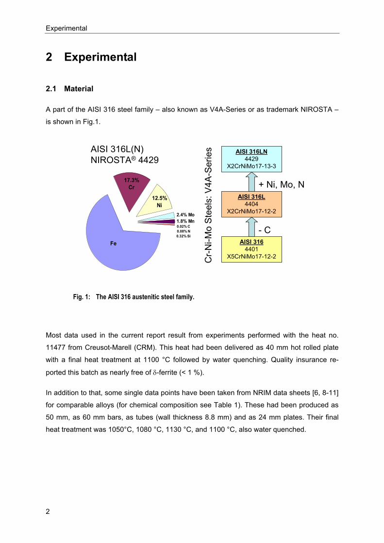
A part of the AISI 316 steel family – also known as V4A-Series or as trademark NIROSTA –
is shown in Fig.1.
Most data used in the current report result from experiments performed with the heat no.
11477 from Creusot-Marell (CRM). This heat had been delivered as 40 mm hot rolled plate
with a final heat treatment at 1100 °C followed by water quenching. Quality insurance re-
ported this batch as nearly free of δ-ferrite (< 1 %).
In addition to that, some single data points have been taken from NRIM data sheets [6, 8-11]
for comparable alloys (for chemical composition see Table 1). These had been produced as
50 mm, as 60 mm bars, as tubes (wall thickness 8.8 mm) and as 24 mm plates. Their final
heat treatment was 1050°C, 1080 °C, 1130 °C, and 1100 °C, also water quenched.
Fe
17.3%Cr
12.5%Ni
2.4% Mo1.8% Mn0.02% C0.08% N0.32% Si
AISI 316L(N)NIROSTA® 4429
Cr-
Ni-M
o S
teel
s: V
4A-S
erie
s
AISI 3164401
X5CrNiMo17-12-2
AISI 316L4404
X2CrNiMo17-12-2
AISI 316LN4429
X2CrNiMo17-13-3
- C
+ Ni, Mo, N
Fig. 1: The AISI 316 austenitic steel family.
Experimental
3
Table 1: Chemical composition of different AISI 316 L(N) steels in wt. per cent.
Alloy C Si Mn P S Cr Ni Mo Cu N Al B
CRM 11477 0.02 0.32 1.80 0.02 0.006 17.34 12.50 2.40 0.12 0.08 0.018 0.0014
SUS 316-B ADA
0.06 0.46 1.49 0.03 0.026 17.43 12.48 2.49 0.15 0.019 0.025 0.0008
SUS 316-H
TB AAL 0.07 0.61 1.65 0.03 0.007 16.60 13.6 2.33 0.26 0.025 0.017 0.0011
2.2 Equipment, Specimens, Test Procedure, and Evaluation
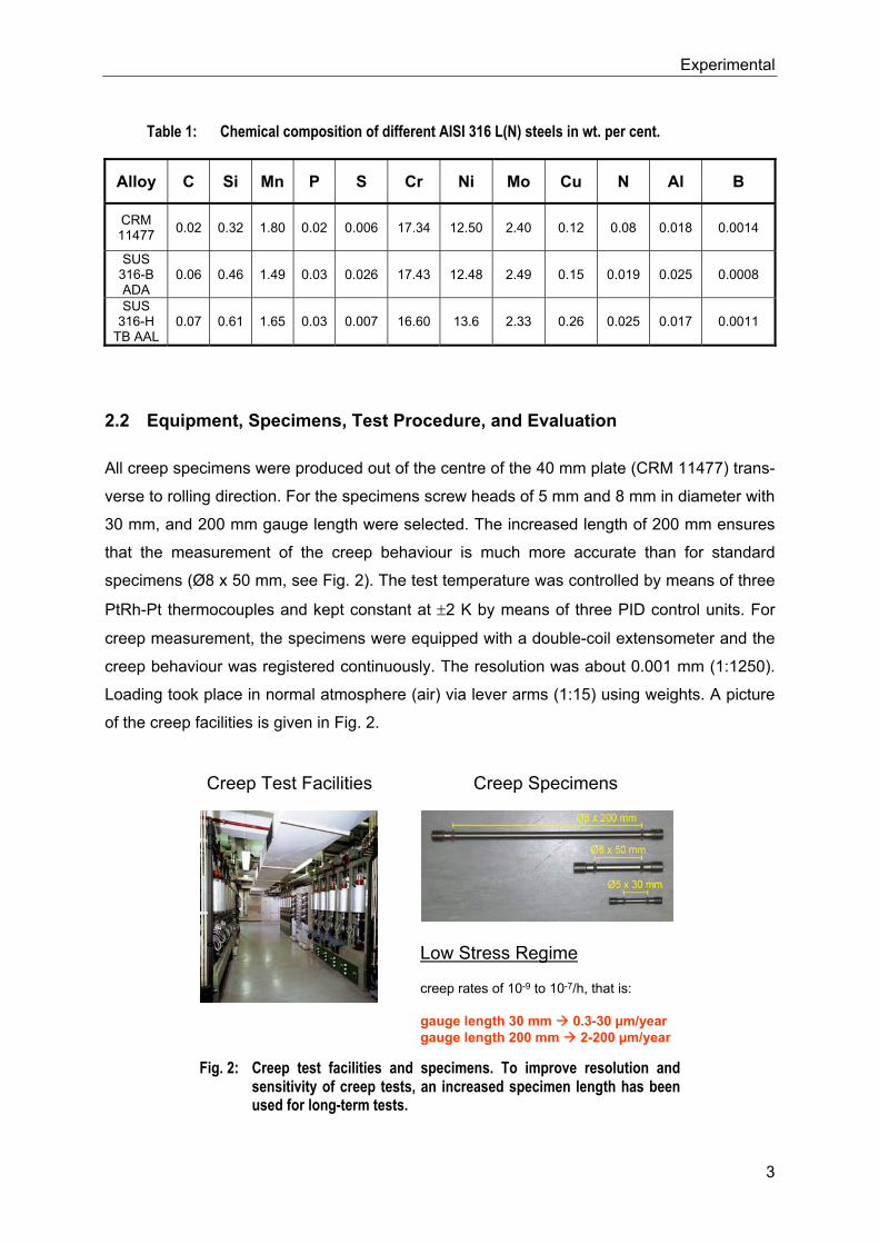
All creep specimens were produced out of the centre of the 40 mm plate (CRM 11477) trans-
verse to rolling direction. For the specimens screw heads of 5 mm and 8 mm in diameter with
30 mm, and 200 mm gauge length were selected. The increased length of 200 mm ensures
that the measurement of the creep behaviour is much more accurate than for standard
specimens (Ø8 x 50 mm, see Fig. 2). The test temperature was controlled by means of three
PtRh-Pt thermocouples and kept constant at ±2 K by means of three PID control units. For
creep measurement, the specimens were equipped with a double-coil extensometer and the
creep behaviour was registered continuously. The resolution was about 0.001 mm (1:1250).
Loading took place in normal atmosphere (air) via lever arms (1:15) using weights. A picture
of the creep facilities is given in Fig. 2.
Creep Test Facilities Creep Specimens
Low Stress Regime
creep rates of 10-9 to 10-7/h, that is:
gauge length 30 mm 0.3-30 µm/yeargauge length 200 mm 2-200 µm/year
Fig. 2: Creep test facilities and specimens. To improve resolution and sensitivity of creep tests, an increased specimen length has been used for long-term tests.
Experimental
4
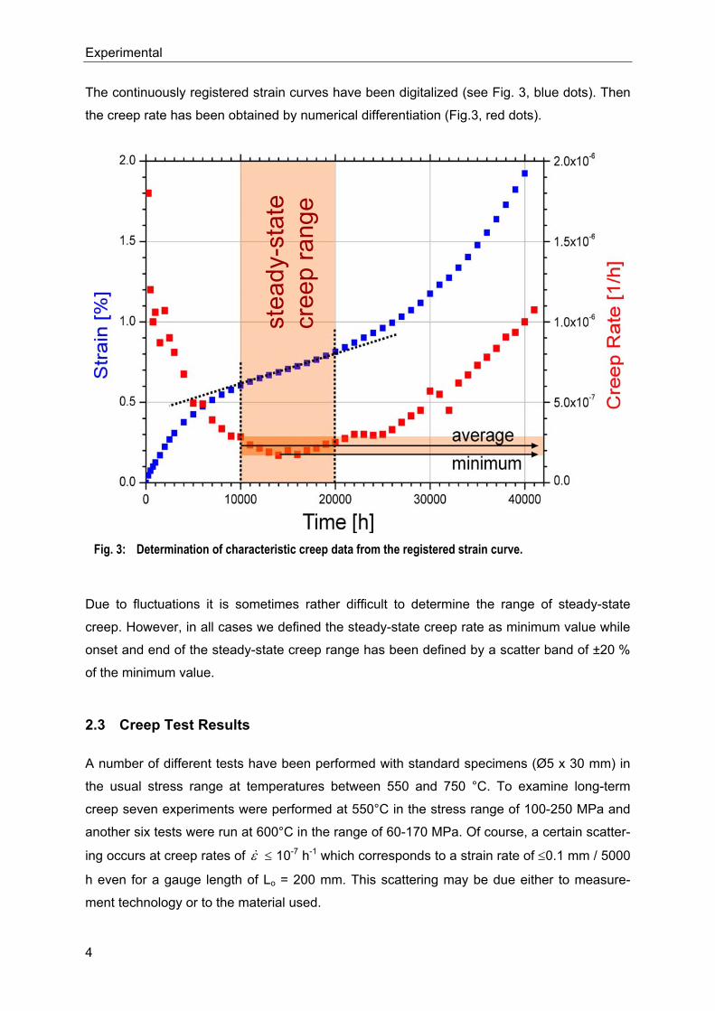
The continuously registered strain curves have been digitalized (see Fig. 3, blue dots). Then
the creep rate has been obtained by numerical differentiation (Fig.3, red dots).
Due to fluctuations it is sometimes rather difficult to determine the range of steady-state
creep. However, in all cases we defined the steady-state creep rate as minimum value while
onset and end of the steady-state creep range has been defined by a scatter band of ±20 %
of the minimum value.
2.3 Creep Test Results
A number of different tests have been performed with standard specimens (Ø5 x 30 mm) in
the usual stress range at temperatures between 550 and 750 °C. To examine long-term
creep seven experiments were performed at 550°C in the stress range of 100-250 MPa and
another six tests were run at 600°C in the range of 60-170 MPa. Of course, a certain scatter-
ing occurs at creep rates of ε& ≤ 10-7 h-1 which corresponds to a strain rate of ≤0.1 mm / 5000
h even for a gauge length of Lo = 200 mm. This scattering may be due either to measure-
ment technology or to the material used.
stea
dy-s
tate
cree
pra
nge
Fig. 3: Determination of characteristic creep data from the registered strain curve.
Experimental
5
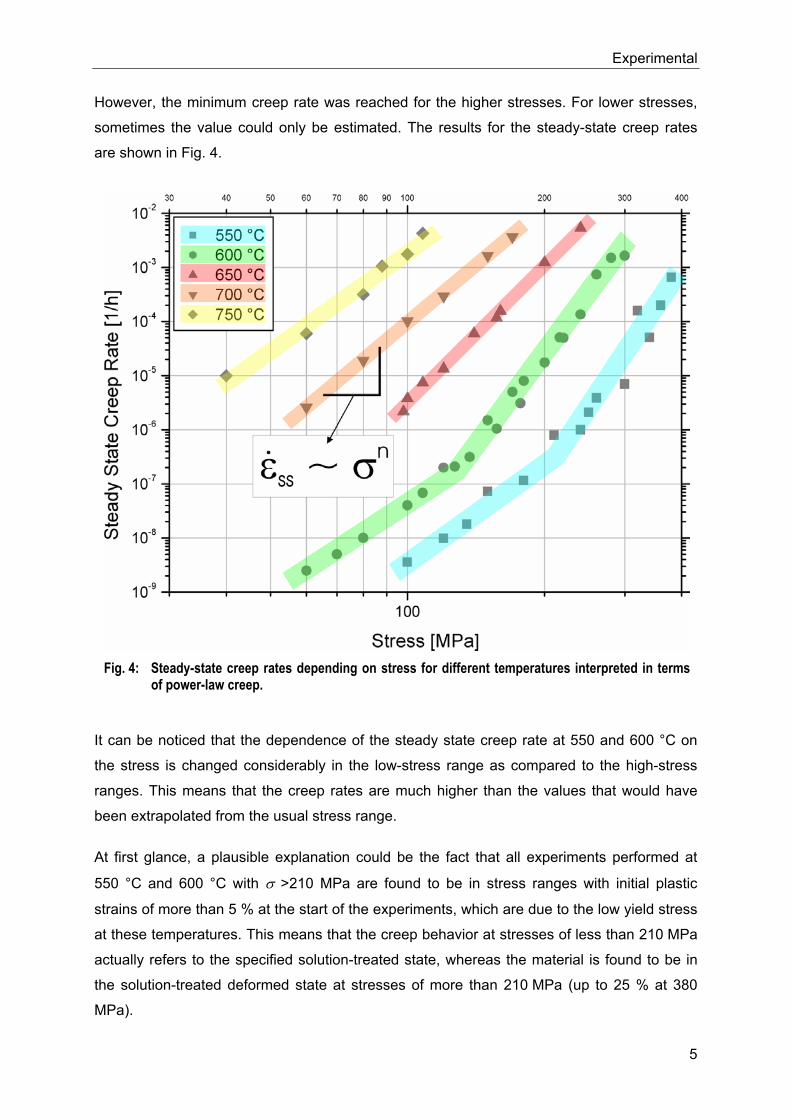
However, the minimum creep rate was reached for the higher stresses. For lower stresses,
sometimes the value could only be estimated. The results for the steady-state creep rates
are shown in Fig. 4.
It can be noticed that the dependence of the steady state creep rate at 550 and 600 °C on
the stress is changed considerably in the low-stress range as compared to the high-stress
ranges. This means that the creep rates are much higher than the values that would have
been extrapolated from the usual stress range.
At first glance, a plausible explanation could be the fact that all experiments performed at
550 °C and 600 °C with σ >210 MPa are found to be in stress ranges with initial plastic
strains of more than 5 % at the start of the experiments, which are due to the low yield stress
at these temperatures. This means that the creep behavior at stresses of less than 210 MPa
actually refers to the specified solution-treated state, whereas the material is found to be in
the solution-treated deformed state at stresses of more than 210 MPa (up to 25 % at 380
MPa).
Fig. 4: Steady-state creep rates depending on stress for different temperatures interpreted in terms of power-law creep.
Experimental
6
It was already demonstrated by several experiments with the Mo-free steel X6CrNi 1811
(corresponding to AISI 304) that this plastic deformation at the start of the tests acts like a
preceding cold deformation [12]. Cold deformation of specimens by 12 % prior to the test or
deformation by 12 % at the test temperature resulted in creep and strength values which
were similar to those obtained for solution-treated specimens with initial strains of more than
10% at the start of the experiments. Therefore, it might be assumed that the observed
change of the steady-state creep rate at lower stresses could result from this experimentally
build-in cold work. However, in Section 3 another explanation will be favored.
2.4 Microstructure
Quite another but also reasonable description could be the change of the microstructure with
time since austenitic stainless steels are well known for their thermal instability at higher tem-
peratures.
100 x 500 x
100 x 500 x
rolli
ngte
xtur
e
rolling texture
100 x 500 x
rolli
ngte
xtur
e
rolling texture
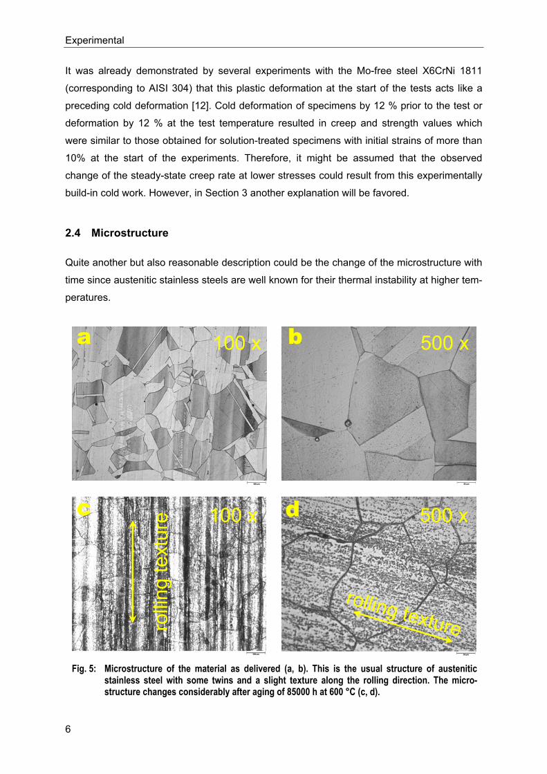
Fig. 5: Microstructure of the material as delivered (a, b). This is the usual structure of austenitic stainless steel with some twins and a slight texture along the rolling direction. The micro-structure changes considerably after aging of 85000 h at 600 °C (c, d).
a b
c d
Experimental
7
Figure 5 a, b shows the microstructure of the 316 L(N) steel in the condition as delivered. In
general there is nothing unusual. Typical twin formations are recognizable as well as a slight
texture along the rolling direction combined with a few rather small inclusions. Other investi-
gations have also shown small parts of delta ferrite.
After aging at 600 °C for 85000 h the microstructure has changed considerably (Fig. 5 c, d).
Precipitations have formed mainly at grain boundaries and along the rolling texture.
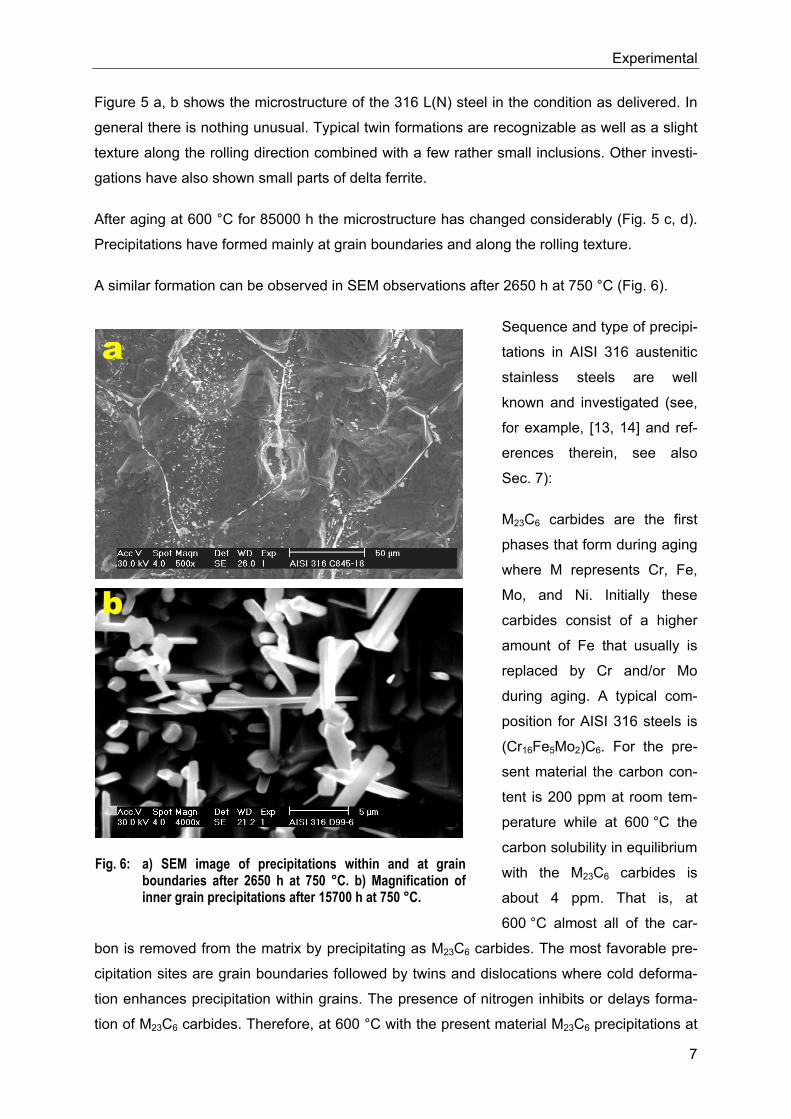
A similar formation can be observed in SEM observations after 2650 h at 750 °C (Fig. 6).
Sequence and type of precipi-
tations in AISI 316 austenitic
stainless steels are well
known and investigated (see,
for example, [13, 14] and ref-
erences therein, see also
Sec. 7):
M23C6 carbides are the first
phases that form during aging
where M represents Cr, Fe,
Mo, and Ni. Initially these
carbides consist of a higher
amount of Fe that usually is
replaced by Cr and/or Mo
during aging. A typical com-
position for AISI 316 steels is
(Cr16Fe5Mo2)C6. For the pre-
sent material the carbon con-
tent is 200 ppm at room tem-
perature while at 600 °C the
carbon solubility in equilibrium
with the M23C6 carbides is
about 4 ppm. That is, at
600 °C almost all of the car-
bon is removed from the matrix by precipitating as M23C6 carbides. The most favorable pre-
cipitation sites are grain boundaries followed by twins and dislocations where cold deforma-
tion enhances precipitation within grains. The presence of nitrogen inhibits or delays forma-
tion of M23C6 carbides. Therefore, at 600 °C with the present material M23C6 precipitations at
Fig. 6: a) SEM image of precipitations within and at grain
boundaries after 2650 h at 750 °C. b) Magnification of inner grain precipitations after 15700 h at 750 °C.
a
b
Experimental
8
grain boundaries start after only a few hundred hours and the formation of carbides within
grains takes even 1000 hours and more.
Due to the small amount of carbon only a minor part of the precipitations shown in Figs. 5
and 6 can be explained by M23C6 carbides. Besides carbide precipitation, during long-term
aging (especially at higher temperatures) AISI 316 steels are prone to formation of intermet-
allic phases. Below 800 °C usually M23C6 precipitation is followed by precipitation of Laves
phase.
grain boundary
grain boundary
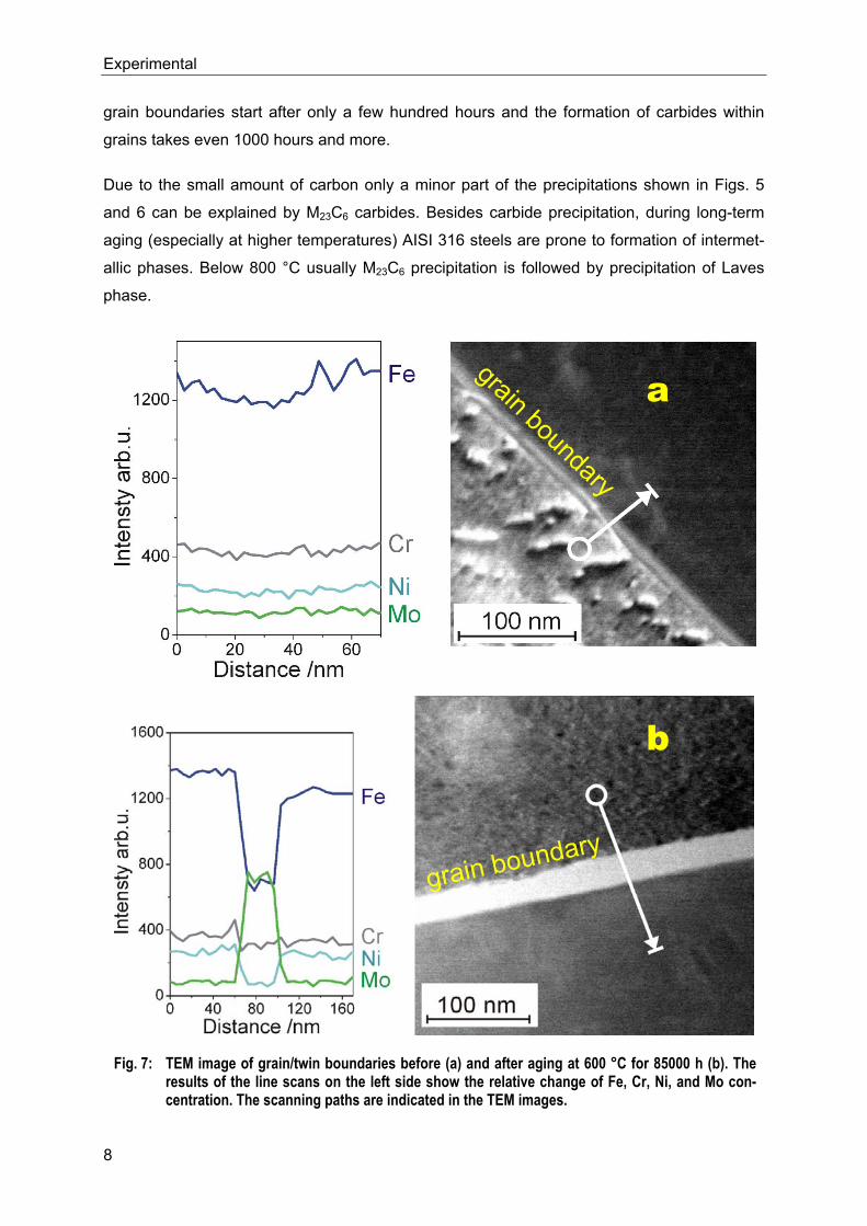
Fig. 7: TEM image of grain/twin boundaries before (a) and after aging at 600 °C for 85000 h (b). The
results of the line scans on the left side show the relative change of Fe, Cr, Ni, and Mo con-centration. The scanning paths are indicated in the TEM images.
a
b
Experimental
9
In the case of the AISI 316 L(N) austenitic steel Laves phase consisting of Fe2Mo starts to
form after aging at 600 °C for about 10000 h first at grain boundaries and finally within grains.
An example is given in Fig. 7 where the intensity drop of the Fe signal and the rise of the Mo
signal lead to a Fe/Mo ratio of about 1:1 after analyzing the TEM signals.
The last phase to appear is the sigma phase. It has a very slow kinetics when forming from
austenite and, therefore, takes aging of about 100000 h at 600 °C. But formation from ferrite
is about 100 times faster. This is another reason why δ-ferrite is undesirable in austenitic
steels. However, the composition of sigma phase in AISI 316 L(N) steels can be approxi-
mated by (Fe, Ni)3 (Cr, Mo)2 or in wt%: 55Fe-29Cr-11Mo-5Ni. Sigma phase precipitates
mainly on grain boundaries (especially on triple junctions) and on intragranular inclusions.
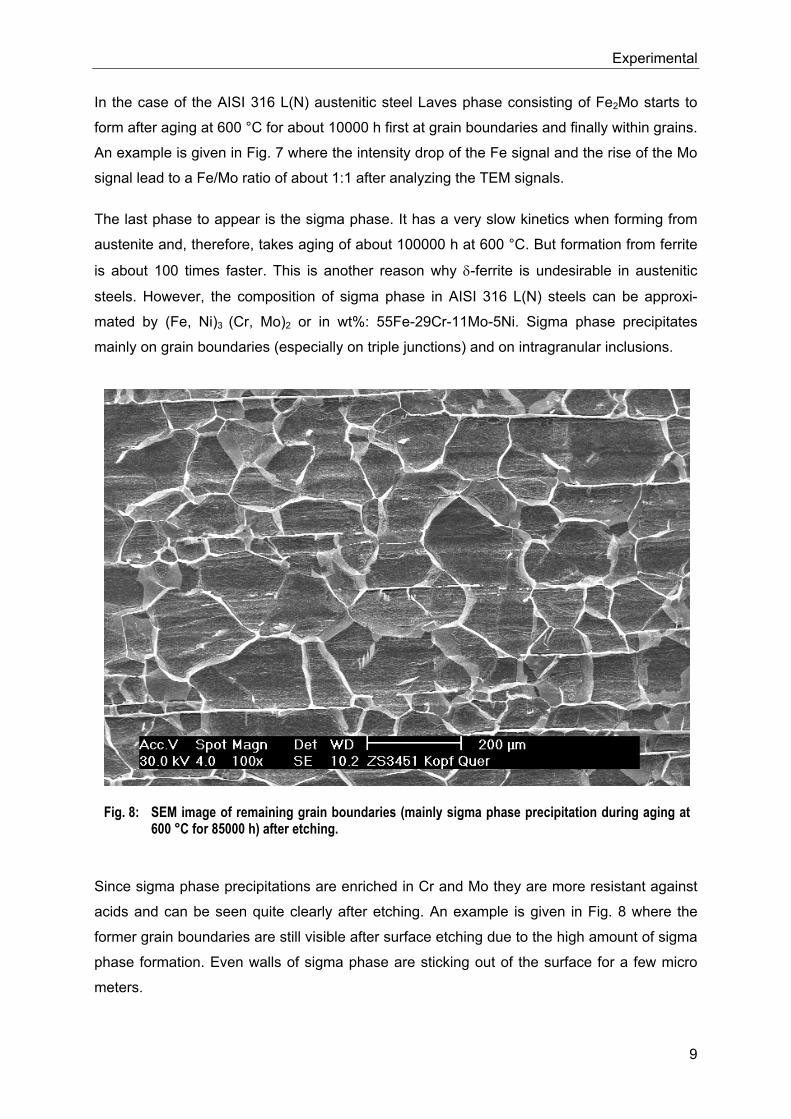
Since sigma phase precipitations are enriched in Cr and Mo they are more resistant against
acids and can be seen quite clearly after etching. An example is given in Fig. 8 where the
former grain boundaries are still visible after surface etching due to the high amount of sigma
phase formation. Even walls of sigma phase are sticking out of the surface for a few micro
meters.
Fig. 8: SEM image of remaining grain boundaries (mainly sigma phase precipitation during aging at
600 °C for 85000 h) after etching.
Experimental
10
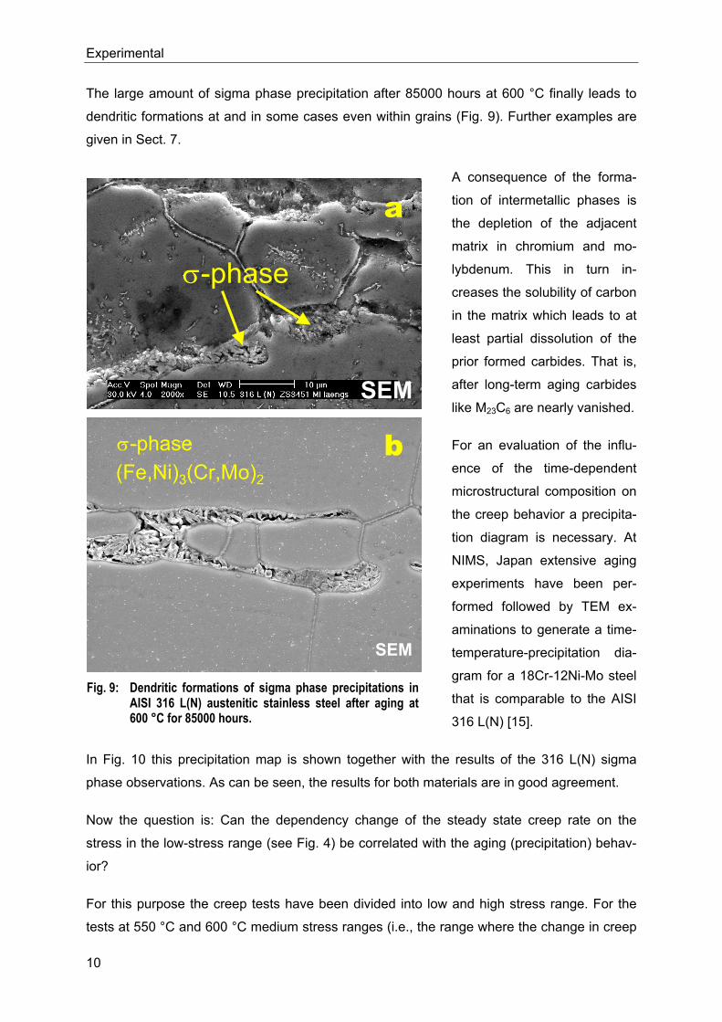
The large amount of sigma phase precipitation after 85000 hours at 600 °C finally leads to
dendritic formations at and in some cases even within grains (Fig. 9). Further examples are
given in Sect. 7.
A consequence of the forma-
tion of intermetallic phases is
the depletion of the adjacent
matrix in chromium and mo-
lybdenum. This in turn in-
creases the solubility of carbon
in the matrix which leads to at
least partial dissolution of the
prior formed carbides. That is,
after long-term aging carbides
like M23C6 are nearly vanished.
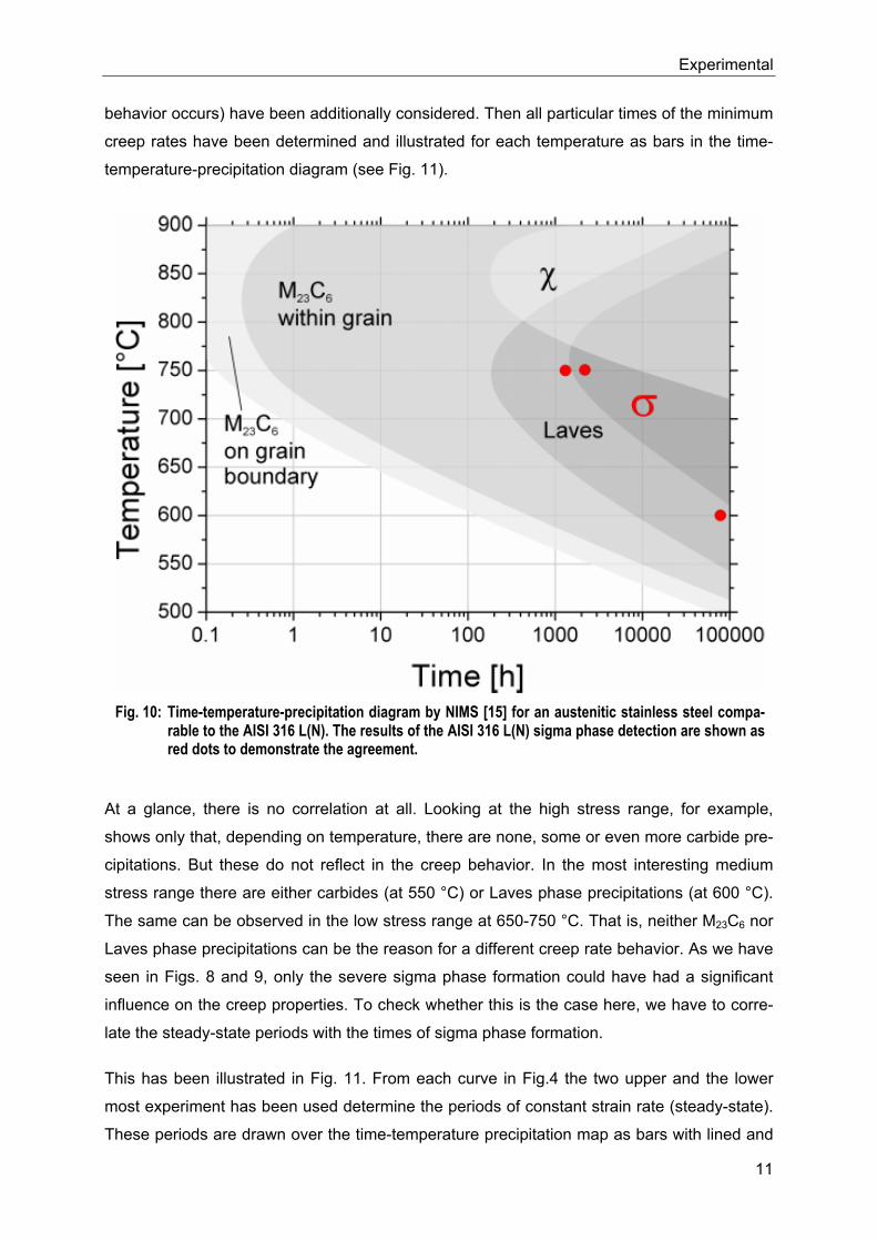
For an evaluation of the influ-
ence of the time-dependent
microstructural composition on
the creep behavior a precipita-
tion diagram is necessary. At
NIMS, Japan extensive aging
experiments have been per-
formed followed by TEM ex-
aminations to generate a time-
temperature-precipitation dia-
gram for a 18Cr-12Ni-Mo steel
that is comparable to the AISI
316 L(N) [15].
In Fig. 10 this precipitation map is shown together with the results of the 316 L(N) sigma
phase observations. As can be seen, the results for both materials are in good agreement.
Now the question is: Can the dependency change of the steady state creep rate on the
stress in the low-stress range (see Fig. 4) be correlated with the aging (precipitation) behav-
ior?
For this purpose the creep tests have been divided into low and high stress range. For the
tests at 550 °C and 600 °C medium stress ranges (i.e., the range where the change in creep
σ-phase
SEM
σ-phase
SEM
(Fe,Ni)3(Cr,Mo)2
Fig. 9: Dendritic formations of sigma phase precipitations in AISI 316 L(N) austenitic stainless steel after aging at 600 °C for 85000 hours.
a
b
Experimental
11
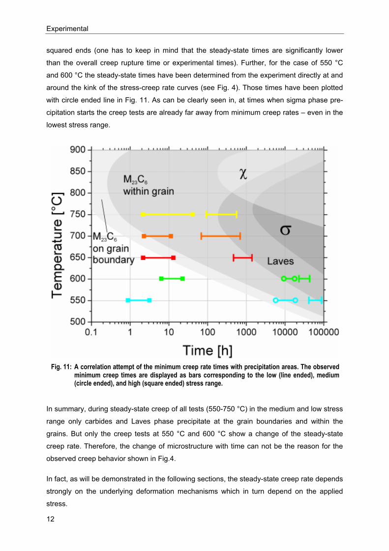
behavior occurs) have been additionally considered. Then all particular times of the minimum
creep rates have been determined and illustrated for each temperature as bars in the time-
temperature-precipitation diagram (see Fig. 11).
At a glance, there is no correlation at all. Looking at the high stress range, for example,
shows only that, depending on temperature, there are none, some or even more carbide pre-
cipitations. But these do not reflect in the creep behavior. In the most interesting medium
stress range there are either carbides (at 550 °C) or Laves phase precipitations (at 600 °C).
The same can be observed in the low stress range at 650-750 °C. That is, neither M23C6 nor
Laves phase precipitations can be the reason for a different creep rate behavior. As we have
seen in Figs. 8 and 9, only the severe sigma phase formation could have had a significant
influence on the creep properties. To check whether this is the case here, we have to corre-
late the steady-state periods with the times of sigma phase formation.
This has been illustrated in Fig. 11. From each curve in Fig.4 the two upper and the lower
most experiment has been used determine the periods of constant strain rate (steady-state).
These periods are drawn over the time-temperature precipitation map as bars with lined and
Fig. 10: Time-temperature-precipitation diagram by NIMS [15] for an austenitic stainless steel compa-rable to the AISI 316 L(N). The results of the AISI 316 L(N) sigma phase detection are shown as red dots to demonstrate the agreement.
Experimental
12
squared ends (one has to keep in mind that the steady-state times are significantly lower
than the overall creep rupture time or experimental times). Further, for the case of 550 °C
and 600 °C the steady-state times have been determined from the experiment directly at and
around the kink of the stress-creep rate curves (see Fig. 4). Those times have been plotted
with circle ended line in Fig. 11. As can be clearly seen in, at times when sigma phase pre-
cipitation starts the creep tests are already far away from minimum creep rates – even in the
lowest stress range.
In summary, during steady-state creep of all tests (550-750 °C) in the medium and low stress
range only carbides and Laves phase precipitate at the grain boundaries and within the
grains. But only the creep tests at 550 °C and 600 °C show a change of the steady-state
creep rate. Therefore, the change of microstructure with time can not be the reason for the
observed creep behavior shown in Fig.4.
In fact, as will be demonstrated in the following sections, the steady-state creep rate depends
strongly on the underlying deformation mechanisms which in turn depend on the applied
stress.
Fig. 11: A correlation attempt of the minimum creep rate times with precipitation areas. The observed minimum creep times are displayed as bars corresponding to the low (line ended), medium (circle ended), and high (square ended) stress range.
Deformation Mechanisms
13
3 Deformation Mechanisms
3.1 Overview
Crystalline solids deform plastically by a number of different and sometimes competing
mechanisms. Although it is often convenient to describe a polycrystalline solid by a well de-
fined yield strength, below which it doesn’t flow and above which flow is rapid, this is only
true at zero temperature. But plastic flow is a kinetic process and in general, the strength of
solids depends on both strain and strain rate, as well as on temperature. It is determined by
all the atomic processes that occur on the atomic scale like, for example, the glide motion of
dislocation lines, the combined climb and glide of dislocations, the diffusive flow of individual
atoms, the relative displacement of grains by grain boundary sliding including diffusion and
defect motion in the boundaries, mechanical twinning by the motion of twinning dislocations,
and so on [16].
But it is more convenient to describe the plasticity of polycrystalline solids in terms of the
mechanisms to which the atomistic processes contribute. Often the deformation mechanisms
are divided into five groups [16]:
• Diffusional Flow (Diffusion Creep) – based on either (a) lattice diffusion (Nabarro-
Herring creep) or (b) grain boundary diffusion (Coble creep).
• Power-law Creep (Dislocation Creep) – diffusion controlled climb-plus-glide proc-
esses: (a) based on lattice diffusion controlled dislocation climb (high temperature
creep), (b) based on core diffusion controlled dislocation climb (low temperature
creep), (c) transition from climb-plus-glide to glide alone (power-law breakdown).
• Mechanical Twinning – low temperature plasticity by the motion of twinning disloca-
tions.
• Dislocation Glide – low temperature plasticity based on dislocation glide, limited by
(a) discrete obstacles or (b) by lattice resistance.
• Elastic Collapse – flow for stresses above the ideal shear strength.
Some mechanisms which are not important for the present material (e.g. Harper-Dorn creep
or creep based on recrystallization) have been left out.
Deformation Mechanisms
14
Plastic flow of fully dense solids is caused by the shear stress σs (deviatoric part of the stress
field). In terms of the principal stresses σ1, σ2 and σ3 :
( ) ( ) ( )[ ]213
232
2216
1 σσσσσσσ −+−+−=s . (1)
It exerts forces on defects (dislocations, vacancies, etc.) in the solid and causes them to
move. The defects are the carriers of deformation and, therefore, the shear strain rate γ&
depends on density and velocity of these deformation carriers. In terms of the principal strain
rates 1ε& , 2ε& and 3ε& it is given by:
. ( ) ( ) ( )[ ]213
232
2212
3 εεεεεεγ &&&&&&& −+−+−= (2)
For simple tension, σs and γ& are related to the tensile stress σ1 and strain rate 1ε& by:
11 3,3
1 εγσσ && ==s . (3)
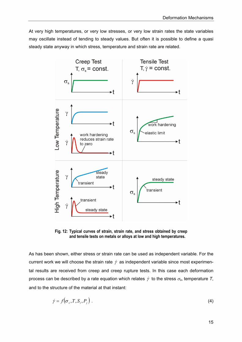
Macroscopic variables of plastic deformation are stress σs, temperature T, strain rate γ& ,
strain γ and time t. During creep or creep rupture tests the stress and temperature are pre-
scribed. Typically forms of strain and strain rate are shown in Fig. 12. At low temperatures of
about 0.1 TM (melting point TM) the material undergoes work hardening until the flow strength
equals the applied stress. During this process its structure changes: the dislocation density
increases, therefore, further dislocation motion is blocked, the strain rate decreases to zero,
and the strain tends asymptotically to a fixed value. During tensile tests the strain rate and
temperature are prescribed. At low temperatures the stress rises as the dislocation density
rises (Fig. 12). That is, for a given set of state variables Si (dislocation density, dislocation
arrangement, cell size, grain size, precipitate size, precipitate distribution, and so on) the
strength is determined by γ& and T, or the strain rate is determined by σs and T.
At higher temperatures (about 0.5 TM) polycrystalline materials creep (see Fig. 12). After a
transient during which the state variables change, a steady state may be reached. During the
steady state the solid continues to deform with no further (significant) change in Si. Here the
state variables Si depend on stress, temperature, and strain rate and a relationship between
these three macroscopic variables may be given.
Deformation Mechanisms
15
At very high temperatures, or very low stresses, or very low strain rates the state variables
may oscillate instead of tending to steady values. But often it is possible to define a quasi
steady state anyway in which stress, temperature and strain rate are related.
As has been shown, either stress or strain rate can be used as independent variable. For the
current work we will choose the strain rate γ& as independent variable since most experimen-
tal results are received from creep and creep rupture tests. In this case each deformation
process can be described by a rate equation which relates γ& to the stress σs, temperature T,
and to the structure of the material at that instant:
( )jis PSTf ,,,σγ =& . (4)
Fig. 12: Typical curves of strain, strain rate, and stress obtained by creep and tensile tests on metals or alloys at low and high temperatures.
Deformation Mechanisms
16
As already mentioned, the set of i quantities Si are the state variables which describe the
current microstructural state of the solid. The set of j quantities Pj are material properties like
lattice parameter, atomic volume, bond energies, moduli, diffusion constants, and so on.
Most often these can be considered as constant.
But the state variables Si generally change during the deformation processes (except in
steady state). So a second set of equations is needed to describe their rate of change:
( )jisii PSTg
dtdS
,,,σ= . (5)
The coupled set of equations (4) and (5) are the constitutive law for a deformation mecha-
nism. They can be solved with respect to time to give the strain after any loading history. But
while there are satisfactory models for the rate equation (4), there is still lack of understand-
ing the structural evolution with strain or time. Therefore a sufficient description of the equa-
tion set (5) is not possible at present.
However, to proceed further, simplifying assumptions about the structure have to be made.
Here are two possible alternatives. A very simple assumption is that of constant structure:
0ii SS = . (6)
Then the rate equation for γ& completely describes plasticity. The second assumption is that
of steady state:
0=dtdSi . (7)
In this case the internal variables no longer appear explicitly in the rate equations. They are
determined by the external variables of stress and temperature. Either simplification reduces
the constitutive law to a single equation:
( )Tf s ,σγ =& , (8)
since, for a given material the properties Pj are constant and the state variables are either
constant or determined by σs and T.
In the following sections rate equations in the form of Eq. (8) are assembled for each of the
deformation mechanisms (i.e., we consider only steady state creep).
Deformation Mechanisms
17
3.2 Diffusional Flow (Diffusion Creep)
3.2.1 Nabarro-Herring Creep
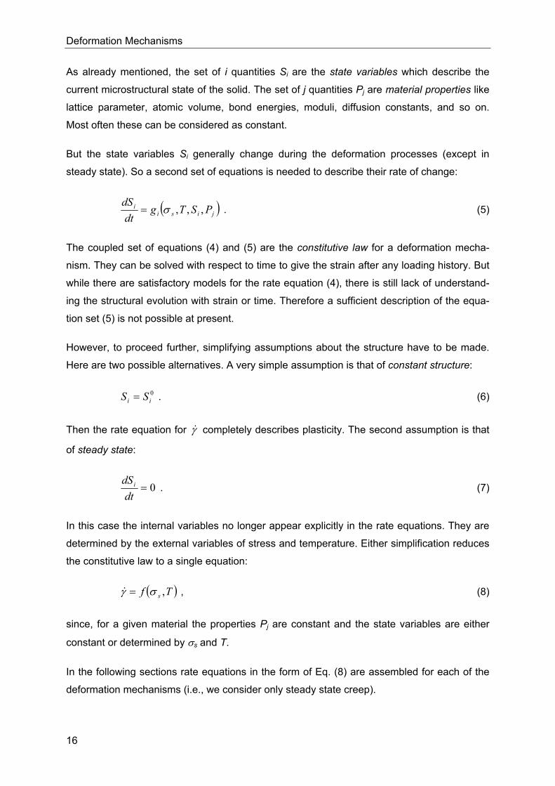
Nabarro and Herring developed a model that describes viscous creep by stress-induced dif-
fusion of vacancies [17, 18]. This mechanism applies to polycrystalline metals at high tem-
peratures where all dislocations are assumed to be pinned and grain boundaries are consid-
ered as distinguished sources or sinks for vacancies.
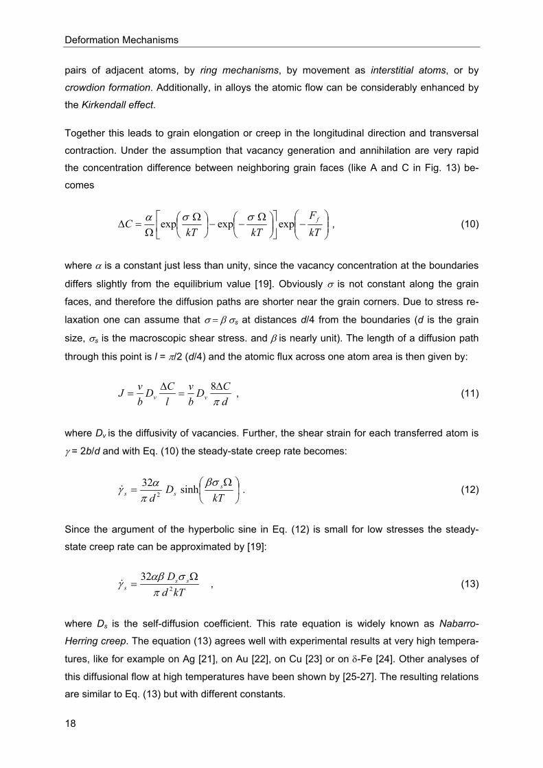
By a stress σ normal to a boundary, vacancy formation is promoted, because the work nec-
essary to form a vacancy is reduced by the amount σ Ω, where Ω is the volume of the va-
cancy (Ω ≈ b³) and b is the magni-
tude of Burgers´ vector). The equi-
librium probability of finding a va-
cancy near a grain boundary (e.g.
surface A and B in Fig. 13) is
given by [19]:
Ω
−=
kTkT
FNN f
S
V σ
σ
expexp .
(9)
Here NV is the number of vacan-
cies for NS lattice sites and Ff is
the free energy for vacancy forma-
tion. If a grain is loaded by normal
stresses σ (see Fig. 13), then the
vicinity of faces A and B show
vacancy concentrations
~exp(σ Ω/kT) while the immediate
surroundings of faces C and D have concentrations ~exp(-σ Ω/kT). Therefore a concentration
gradient is established which causes a vacancy flow from A and B to C and D [19] as indi-
cated in Fig. 13.
Simultaneously the vacancy flow is accompanied by a matching flow of atoms in the opposite
direction (see Fig. 13). The mechanisms for these combined flows are well known (see for
example [20]): The possibilities for diffusive atomic movements are by direct interchange of
Fig. 13: Vacancy flow (red) and opposed atom flow (blue) in a grain under tensile and compressive stress (schematic drawing).
Deformation Mechanisms
18
pairs of adjacent atoms, by ring mechanisms, by movement as interstitial atoms, or by
crowdion formation. Additionally, in alloys the atomic flow can be considerably enhanced by
the Kirkendall effect.
Together this leads to grain elongation or creep in the longitudinal direction and transversal
contraction. Under the assumption that vacancy generation and annihilation are very rapid
the concentration difference between neighboring grain faces (like A and C in Fig. 13) be-
comes
−
Ω
−−
Ω
Ω=∆
kTF
kTkTC fexpexpexp σσα
, (10)
where α is a constant just less than unity, since the vacancy concentration at the boundaries
differs slightly from the equilibrium value [19]. Obviously σ is not constant along the grain
faces, and therefore the diffusion paths are shorter near the grain corners. Due to stress re-
laxation one can assume that σ = β σs at distances d/4 from the boundaries (d is the grain
size, σs is the macroscopic shear stress. and β is nearly unit). The length of a diffusion path
through this point is l = π/2 (d/4) and the atomic flux across one atom area is then given by:
dCD
bv
lCD
bvJ vv π
∆=
∆=
8 , (11)
where Dv is the diffusivity of vacancies. Further, the shear strain for each transferred atom is
γ = 2b/d and with Eq. (10) the steady-state creep rate becomes:
Ω
=kT
Dd
sss
βσπ
αγ sinh322
& . (12)
Since the argument of the hyperbolic sine in Eq. (12) is small for low stresses the steady-
state creep rate can be approximated by [19]:
kTdD ss
s 2
32π
σαβγ
Ω=& , (13)
where Ds is the self-diffusion coefficient. This rate equation is widely known as Nabarro-
Herring creep. The equation (13) agrees well with experimental results at very high tempera-
tures, like for example on Ag [21], on Au [22], on Cu [23] or on δ-Fe [24]. Other analyses of
this diffusional flow at high temperatures have been shown by [25-27]. The resulting relations
are similar to Eq. (13) but with different constants.
Deformation Mechanisms
19
3.2.2 Coble Creep
Self-diffusion in poly crystals comprises two mechanisms: lattice and grain boundary diffu-
sion. While lattice diffusion dominates at very high temperatures, grain boundary diffusion
takes over mainly at lower temperatures (see for example [28, 20]). Coble described the dif-
fusional flow at lower temperatures and stresses with the following rate equation (Coble
creep [29]):
Bs
s DkTd 3
42 Ω=
σδπγ& . (14)
Here DB is the boundary diffusion coefficient and δ the effective thickness of the grain bound-
ary.
3.2.3 Alternative Descriptions
In most models for diffusion creep both mechanisms (Eqs. (13) and (14)) are combined in
one rate equation (see, for example, [16]):
effs
s DkTd 2
42 Ω=
σγ& , (15)
with
+=
L
BLeff D
Dd
DD πδ1 . (16)
Here DL is the lattice diffusion coefficient.
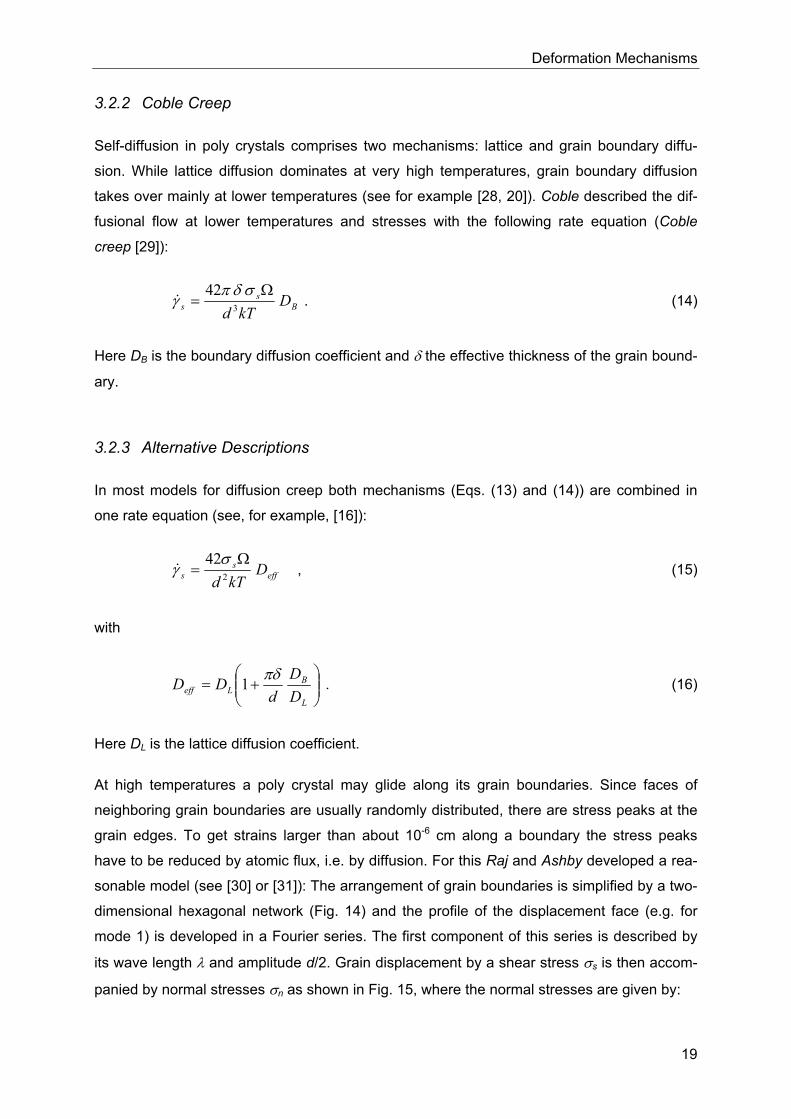
At high temperatures a poly crystal may glide along its grain boundaries. Since faces of
neighboring grain boundaries are usually randomly distributed, there are stress peaks at the
grain edges. To get strains larger than about 10-6 cm along a boundary the stress peaks
have to be reduced by atomic flux, i.e. by diffusion. For this Raj and Ashby developed a rea-
sonable model (see [30] or [31]): The arrangement of grain boundaries is simplified by a two-
dimensional hexagonal network (Fig. 14) and the profile of the displacement face (e.g. for
mode 1) is developed in a Fourier series. The first component of this series is described by
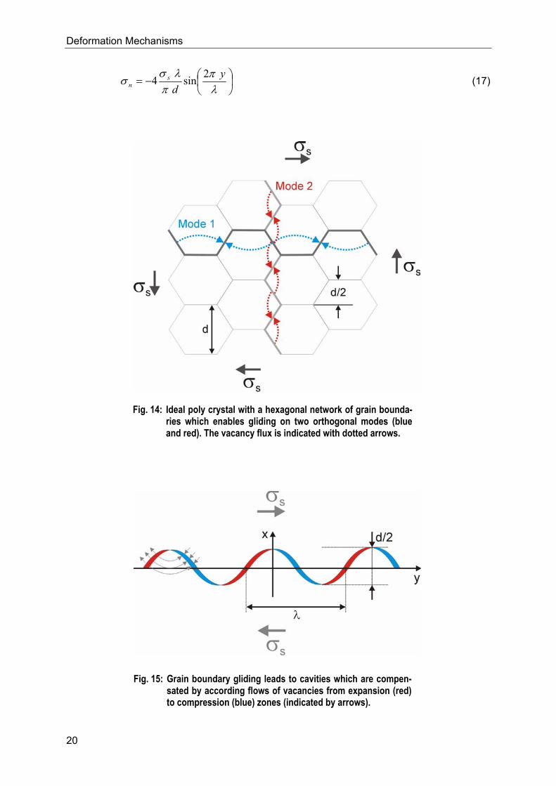
its wave length λ and amplitude d/2. Grain displacement by a shear stress σs is then accom-
panied by normal stresses σn as shown in Fig. 15, where the normal stresses are given by:
Deformation Mechanisms
20
−=
λπ
πλσ
σ yds
n2sin4 (17)
Fig. 14: Ideal poly crystal with a hexagonal network of grain bounda-ries which enables gliding on two orthogonal modes (blue and red). The vacancy flux is indicated with dotted arrows.
Fig. 15: Grain boundary gliding leads to cavities which are compen-sated by according flows of vacancies from expansion (red) to compression (blue) zones (indicated by arrows).
Deformation Mechanisms
21
These normal stresses produce an additional chemical potential for the vacancy generation
∆µ = σn Ω which forces the vacancies to flow from the expansion to the compression zones
at the boundary (see Fig. 15).
This process defines the strain rate at the grain boundary [30, 31]:
+
Ω=
L
BL
ss D
DD
kTd λπδ
πλσ
γ 164
3& . (18)
It is a similar result like that from Nabarro, Herring, and Coble (Eqs. (15) and (16)). But here
the lattice diffusion creep rate depends on λ/d 3 instead of 1/d 2 while the grain boundary
creep rate depends on δ/d 3 in both descriptions. That is, in Eq. (18) lattice diffusion is de-
scribed not only by grain size but by the grain shape (with a shape factor d/λ).
3.3 Power-law Creep (Dislocation Creep)
At high temperatures materials show rate dependent plasticity, or creep. Above 0.3 TM for
pure metals and about 0.4 TM for alloys this dependence on strain rate becomes rather
strong. It may be expressed by an equation of the form:
n
ss
µ
σγ ~& , (19)
where µ is the shear modulus and where n has a value between 3 and 10 in the high tem-
perature regime. Therefore this deformation mechanism is called power-law creep.
3.3.1 Power-law Creep by Climb (plus Glide)
At high temperatures dislocations acquire two degrees of freedom: they can climb as well as
glide. If a gliding dislocation is blocked by discrete obstacles, a little climb may release it,
and, therefore, enable it to glide to the next obstacles where the whole process is repeated.
The glide step is responsible for almost all of the strain, while the average dislocation velocity
is determined by the climb step. Mechanisms which are based on such a climb-plus-glide
sequence are referred to as climb-controlled creep [32-34].
There is an important difference between power-law creep and the deformation mecha-
nisms of the following sections like, for example, dislocation glide (low temperature plastic-
ity, see Section 4.5): the rate-controlling process is the diffusive motion of single ions or va-
Deformation Mechanisms
22
cancies to or from the climbing dislocations, rather than the activated glide of the dislocation
itself. That is, the dominant process takes place at an atomic level.
A steady-state dislocation theory based on the climb of edge dislocations has been proposed
by Weertman [35]. In his proposal it was assumed that work hardening occurs when disloca-
tions are arrested and piled up against existing barriers such as grain boundaries or precipi-
tates. The stress field at the tip of the piled-up dislocations induces multiple slip and the for-
mation of Lomer-Cottrell sessile dislocations anywhere along the original piled-up disloca-
tions. At this point dislocations beyond the Lomer-Cottrell barrier may easily escape by climb.
But climb behind the Lomer-Cottrell barrier would lead to the generation of new dislocation
loops and to a steady-state creep rate. This model can be applied very well to fcc and bcc
metals.
In a further proposal Weertman [36] suggested that edge dislocations of opposite sign gliding
on parallel slip planes would interact and pile up whenever a critical distance between slip
planes is not exceeded. Like in the first model, dislocations may escape from the piled-up
arrays by climb.
Dislocation pile-ups lead to work hardening while climb is a recovery process. Therefore, a
steady-state condition is reached when the hardening and recovery rates are equal. The
creep rate will then be controlled by the rate at which dislocations can climb. On the other
hand, the climb mechanism requires that vacancies be created or destroyed at dislocations
with sufficient ease and that in the vicinity of the dislocations an equilibrium concentration of
vacancies be maintained at a level sufficient to satisfy the climb rate.
At the tip of a pile-up of dislocations a non-vanishing hydrostatic stress may exist which ex-
erts a force on a dislocation in a direction normal to the slip plane and favors up or down
climb. Vacancies are absorbed where the stress is compressive and they are created where
the stress is tensile (compare previous section and Figs. 13-15). This results in a change in
the vacancy concentration near a dislocation line. Therefore, a vacancy flux is established
between segments of dislocations which act as sources and segments acting as sinks.
The vacancy concentration C e in equilibrium with the lead dislocation in a pile-up is given by:
±=
kTbL
CC se µ
σ 22
02
exp , (20)
Deformation Mechanisms
23
where 2L is the length of the dislocation pile-up and C 0 is the equilibrium concentration of
vacancies in a dislocation free crystal. The vacancy concentration at a distance r from each
pile-up is assumed to be equal to C 0. Thus the rate of climb X& is approximated by [19]:
kT
bLDCX sv
µσ 42
02=& , (21)
where Dv is the coefficient for vacancy diffusion and with 2Lb2σs²/µkT < 1. This relation has
been obtained under the assumption that vacancies are easily destroyed or created and that
an equilibrium concentration exists between pile-ups in the vicinity of dislocations. The diffu-
sion problem for the flux of vacancies, however, may be different for specific climbing proc-
esses. Further, if vacancies are only created or destroyed at jogs, the energy of jog formation
has to be taken into account in the case that they are formed by thermal fluctuations. On the
other hand, if these are formed mechanically by intersection, then the rate of climb may still
depend primarily on self-diffusion. This is certainly the case if it is accepted that vacancies
will diffuse rapidly along a dislocation line toward or away from a jog.
For the second model by Weertman the rate of dislocation climb is given also by Eq. (21).
The steady-state creep model in this case becomes:
rXNAbs 2
&& =γ , (22)
where N is the density of dislocations participating in the climb process or – for this model –
the density of sources, A is the area swept out by a loop in the pile-up, and 2r is the separa-
tion between pile-ups. The stress necessary to force two groups of dislocation loops to pass
each other on parallel slip planes has to be greater than µb/4πσs. Thus an estimate of r may
be used with:
s
brπσµ
4= . (23)
Further, the probability p of blocking the dislocation loops generated from one source by
loops emanating from three other loops is given by:
s
bNLpσ
µ3
2 2
= . (24)
Deformation Mechanisms
24
Now the creep rate can be obtained from Eqs. (21)-(24) by setting p=1, A=4πL², and by the
assumption that self-diffusion occurs by vacancy migration. The creep rate at low stresses
becomes [19]:
kTbN
Dc sss 7
5.42
µ
σπγ =& , (25)
where c is a numerical constant of about ¼ and Ds is the coefficient for self-diffusion.
Equation (25) has been proofed experimentally for pure metals at low stresses to a greater
extent than any other theoretical creep relation [19]. Although exceptions exist to the expo-
nent of 4.5 on the stress, this value is remarkably close to observed values. There is general
agreement that high temperature creep is diffusion-controlled and that it depends on Ds. It
was shown for many metals tested at various temperatures [37, 38] that a plot of ln[γ& /Ds]
against ln[σs/µ] reduces the experimental results into a single band, further substantiating Eq.
(25).
On the other hand, there are some points and observations which don’t fit to this theory. It is
questionable whether pile-ups can result from the interaction between edge dislocations of
opposite sign gliding on parallel slip planes. Calculations have shown that the interaction
between such dislocations does not impede their motion. They can cross over each other
and form dipoles which in turn are mobile (see, for example, [39]). Further, in this theory the
number of dislocations in a pile-up is given by 2σsL/µb which predicts extensive pile-ups at
high stresses but not necessarily at low stress levels.
Another deduction of power-law creep based on climb-plus-glide is given in [16] which is
briefly outlined in the following:
Above about 0.6 TM climb is generally lattice-diffusion controlled. The velocity vc at which an
edge dislocation climbs under a local normal stress σn acting parallel to its Burgers’ vector
can be approximated by [40]:
bkT
Dv nLc
Ω≈
σ , (26)
where DL is the lattice diffusion coefficient and Ω the atomic volume. The basic climb-
controlled creep equation may then be obtained under the assumption that σn is proportional
to the applied stress σs and that the average velocity of the dislocation is proportional to the
Deformation Mechanisms
25
rate at which it climbs. With Eq. (26), the Orowan theory [41], and an estimate of the density
of mobile dislocations [42] the creep equation becomes:
3
1
=
µσµ
γ sL
kTbDc& , (27)
with the approximation Ω ≈ b³. All constants are incorporated in c1 which is of order unity.
Some materials – but they are exceptions – obey this equation with a power of 3 and a con-
stant c1 of about 1 [43]. It appears that the local normal stress is not necessarily proportional
to σs implying that dislocations may be moving in a cooperative manner which concentrates
stress. Or the density of mobile dislocations varies in more complicated manner than as-
sumed by [42]. Over a limited range of stress – up to about 10-3 µ – experiments are well
described by a modification of Eq. (27) [44]:
n
sL
kTbDc
=
µσµ
γ 2& , (28)
where the exponent n varies between 3 and about 10. However, present theoretical models
for this behavior are unsatisfactory. None can convincingly explain the observed values of n.
And further, the very large values of the dimensionless constant c2 strongly suggest that
some important physical quantity is still missing from the equation (see, for example, [45,
43]). However, it provides a good description of experimental data and as generalization of
Eq. (27) it has some basis as a physical model.
But Eq. (28) cannot describe the increase of the exponent n and the drop of the activation
energy for creep at lower temperatures which are experimental facts. To incorporate these
observations one has to assume that the transport of matter via dislocation core diffusion
contributes significantly to the overall diffusive transport of matter. And under certain condi-
tions this mechanism should become dominant [46]. A possibility to include the contribution
of core diffusion is the definition of an effective diffusion coefficient (see [47] and [46]):
CCLLeff fDfDD += , (29)
where DC is the core diffusion coefficient, and fC and fL are the fractions of atom sites associ-
ated with each type of diffusion. The value of fL is nearly unity while the value of fC is deter-
mined by the dislocation density ρ:
ρcC af = , (30)
Deformation Mechanisms
26
where ac is the cross-section area of the dislocation core in which fast diffusion is taking
place. Measurements of the quantity ac DC can be found in [48]: the diffusion enhancement
depends on the dislocation orientation (it is probably 10 times larger for edge than for screw
dislocations) and on the degree of dissociation (and therefore on the arrangement of the dis-
locations). Even the activation energy is not constant. But in general, DC is about approxi-
mately equal to the grain boundary diffusion constant DB, if ac is taken to be 2δ ² (δ is the ef-
fective grain boundary thickness). A common experimental observation for the dislocation
density is (see, for example, [42] or [59] for the case of tungsten in the creep regime):
2
2
10
≈
µσ
ρ s
b , (31)
Then the rate equation for power-law creep with an effective diffusion coefficient becomes:
+
=
L
CscL
ns
s DD
baD
kTbc
2
22101
µσ
µσµγ& , (32)
Equation (32) is a combination of two rate equations. At high temperatures and low stresses
lattice diffusion is dominant ( sγ& ~σsn) while at higher stresses (or low temperatures) core dif-
fusion is the dominant process ( sγ& ~σsn+2).
3.3.2 Power-law Breakdown
At high stresses above about 10-3 µ the simple power-law breaks down. The measured strain
rates are significantly greater than predicted by Eq. (32). This process is evidently a transi-
tion from climb-controlled to glide-controlled flow, that is, it is a transition from diffusion-
controlled to thermally activated mechanisms. There have been numerous attempts to de-
scribe it empirically and most descriptions lead to the generalized form ([60, 61, 19]):
( )[ ]
−′RTQ
c crns expsinh~ σγ& , (33)
which reduces to a simple power-law at low stresses (c’σs < 0.8) and which becomes an ex-
ponential at high stresses (c’σs > 1.2).
Measurements of the activation energy Qcr in the power-law breakdown regime often give
values which exceed that of self-diffusion. This might indicate that the recovery process dif-
Deformation Mechanisms
27
fers from that of climb-controlled creep. Some of the difference, however, may simply result
from the temperature dependence of the shear modulus which has a greater effect when the
stress dependence is in the exponential region. Then a better fit to experiment may be found
by [16]:
−
′=
RTQa
A cr
n
s expsinhµσ
γ& , (34)
The equation may be rewritten for an exact correspondence with the power-law equation
(32). Then the rate-equation for both power-law creep and power-law breakdown reads as
follows [16]:
+
′′=L
CscL
n
ss D
Dba
DakTbA
2
2
101sinh
µσ
µσµγ& . (35)
3.4 Mechanical Twinning
Twinning is an important deformation mechanism at low temperatures in hcp and bcc metals
(and some ceramics). In fcc metals (like the austenitic steel AISI 316 considered in this work)
it is less important and occurs only at very low temperatures. The tendency of fcc metals to
twin increases with decreasing stacking fault energy being greatest for silver and completely
absent in aluminium. Therefore, and because existing descriptions are rather uncertain, it is
just mentioned briefly in the following.
Twinning is a variety of dislocation glide involving the motion of partial – instead of complete
– dislocations. The kinetics of the process, however, often indicates that nucleation – and not
propagation – determines the rate flow. Anyway, it may still be possible to describe the strain
rate by a rate equation for twinning by [16]:
−
∆−=
t
sNt kT
Fσσ
γγ 1exp&& . (36)
Here ∆FN is the activation free energy to nucleate a twin without the help of external stress,
tγ& is a constant which includes the density of available nucleation sites and the strain pro-
duced for a successful nucleation, and tσ is the stress required to nucleate twinning in the
Deformation Mechanisms
28
absence of thermal activation. Further the temperature dependence of ∆FN must be included
to explain the observation that the twinning stress may decrease with decreasing tempera-
ture (see [49]).
3.5 Dislocation Glide (Low Temperature Plasticity)
Below the ideal shear strength flow by the conservative or glide motion of dislocations is
possible, provided a sufficient number of independent slip systems is available. This motion
is almost always obstacle-limited, i.e., it is limited by the interaction of potentially mobile dis-
locations with other dislocations, with solute or precipitates, with grain boundaries, or with the
periodic friction of the lattice. These interactions determine the rate of flow and – at a given
rate – the yield strength. Dislocation glide is a kinetic process while dislocation climb (plus
glide) is a diffusion-controlled process, as outlined in Section 4.3. This kinetic process was
first described by Orowan [41]: Mobile dislocations with a density ρm move through a field of
obstacles with an average velocity v ; the velocity is almost entirely determined by their wait-
ing time at the obstacles; the strain rate they produce due to their movement is then given
by:
vbmργ =& , (37)
where b is the magnitude of the Burgers’ vector of a dislocation. At steady state the density
of mobile dislocations ρm is a function of stress and temperature only. The simplest function –
consistent with both theory and experiment – is given by [42]:
2
=
bs
m µσ
αρ , (38)
where α is a constant of order unity. The velocity v depends on the force F acting on the
dislocation by:
bF sσ= , (39)
and on its mobility M:
FMv = . (40)
Now the problem is to calculate M, and therefore v . In the most interesting range of stress M
is determined by the rate at which dislocation segments are thermally activated through or
round obstacles. The next difficulty encounters by the fact that the velocity is always an ex-
Deformation Mechanisms
29
ponential function of stress, but the details of the exponent depend on the shape and nature
of the obstacles. So at first sight there are as many rate equations as there are types of ob-
stacles. But on closer examinations obstacles can be divided in two broad classes: discrete
obstacles and extended, diffuse barriers to dislocation motion.
Examples of the first type are strong dispersoids or precipitates which can be bypassed indi-
vidually by a moving dislocation. Other examples of discrete obstacles are forest dislocations
or weak precipitates which may be cut by dislocation movements. Obstacles of the second
class are concentrated solutions or the lattice itself which leads to lattice-friction.
3.5.1 Plasticity Limited by Discrete Obstacles
The velocity of dislocations in a polycrystal is frequently determined by the strength and den-
sity of the discrete obstacles it contains. If the free energy of activation for cutting or bypass-
ing an obstacle is ∆G(σs), the mean velocity is given by the kinetic equation (see [50-52, 16]):
( )
∆−=
kTG
bv sσνβ exp , (41)
where β is a dimensionless constant and ν is a frequency.
The quantity ∆G(σs) depends on the distribution of obstacles and on the pattern of internal
stress which characterizes one of them. A regular array of box-shaped obstacles – each one
viewed as a circular patch of constant, adverse, internal stress – leads to the simple result
[16]:
( )
−∆=∆
τσ
σˆ
1 ss FG , (42)
where ∆F is total free energy – the activation energy – required to overcome the obstacle
without aid from external stresses. The material property τ is the stress which reduces G∆
to zero, forcing the dislocation through the obstacle without help from thermal energy. It can
be though of as the flow strength of the solid at 0 K.
But obstacles are seldom box-shaped and regularly spaced. Therefore, to describe other
obstacle shapes as well as random distribution, the equation may be rewritten in the follow-
ing way [51]:
Deformation Mechanisms
30
( )qp
ss FG
−∆=∆
τσ
σˆ
1 . (43)
The values of p, q, and ∆F are bounded, i.e., all models lead to values of [16]:
2110
≤≤≤≤
qp
. (44)
The importance of p and q depends on the magnitude of ∆F. When ∆F is large, their influ-
ence is small and their choice is unimportant. Therefore, for discrete obstacles p = q = 1 is a
good choice. But when ∆F is small, the choice becomes more critical. In this case (e.g. for
diffuse obstacles) p and q have to be fitted to the experimental data (see also Section 4.5.2).
The strain rate sensitivity of the strength is determined by ∆F (it characterizes the strength of
a single obstacle). It is helpful to categorize obstacles by their strength as shown in Table 2;
examples for typical values of ∆F are 2 µb³ for large or strong precipitates, and 0.5 µb³ for
pure metals in the work-hardened state.
The quantity τ is the shear strength in the absence of thermal energy. It reflects not only the
strength but also the density and arrangement of the obstacles. For widely spaced, discrete
obstacles τ is proportional to µb/l, where l is the obstacle spacing. The actual value of τ
depends on obstacle strength and distribution (see Table 2). For pure metals strengthened
by work-hardening it can be simply assumed that τ = µb/l.
At this point a combination of all the above listed equations leads to the rate equation for
discrete obstacle controlled plasticity:
−
∆−
=
τσ
µσ
αβνγˆ
1exp2
sss kT
F& . (45)
When ∆F is large (as is normally the case), the stress dependence of the exponential is so
large compared to the pre-exponential 0γ& that it may be set constant for a reasonable fit to
experimental data:
s
s 11062
0 ≈
=
µσ
αβνγ& . (46)
Deformation Mechanisms
31
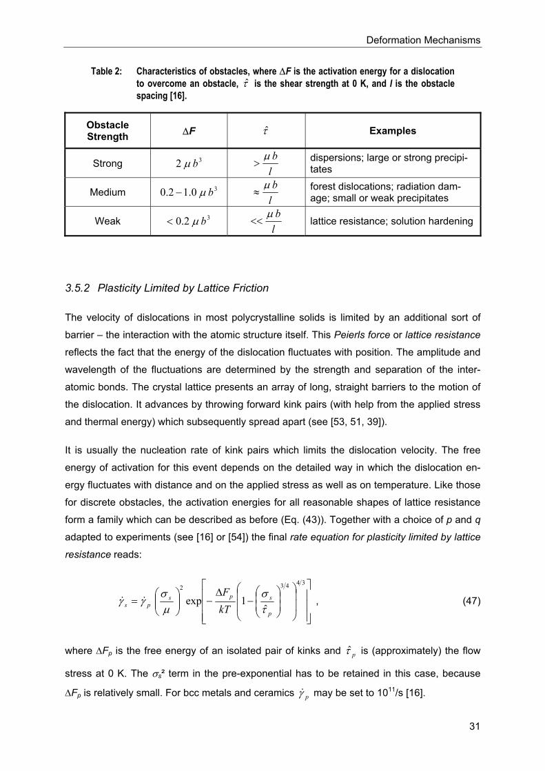
Table 2: Characteristics of obstacles, where ∆F is the activation energy for a dislocation to overcome an obstacle, τ is the shear strength at 0 K, and l is the obstacle spacing [16].
Obstacle Strength ∆F τ Examples
Strong 32 bµ lbµ
> dispersions; large or strong precipi-tates
Medium 30.12.0 bµ− lbµ
≈ forest dislocations; radiation dam-age; small or weak precipitates
Weak 32.0 bµ< lbµ
<< lattice resistance; solution hardening
3.5.2 Plasticity Limited by Lattice Friction
The velocity of dislocations in most polycrystalline solids is limited by an additional sort of
barrier – the interaction with the atomic structure itself. This Peierls force or lattice resistance
reflects the fact that the energy of the dislocation fluctuates with position. The amplitude and
wavelength of the fluctuations are determined by the strength and separation of the inter-
atomic bonds. The crystal lattice presents an array of long, straight barriers to the motion of
the dislocation. It advances by throwing forward kink pairs (with help from the applied stress
and thermal energy) which subsequently spread apart (see [53, 51, 39]).
It is usually the nucleation rate of kink pairs which limits the dislocation velocity. The free
energy of activation for this event depends on the detailed way in which the dislocation en-
ergy fluctuates with distance and on the applied stress as well as on temperature. Like those
for discrete obstacles, the activation energies for all reasonable shapes of lattice resistance
form a family which can be described as before (Eq. (43)). Together with a choice of p and q
adapted to experiments (see [16] or [54]) the final rate equation for plasticity limited by lattice
resistance reads:
−
∆−
=
34432
ˆ1exp
p
spsps kT
Fτσ
µσ
γγ && , (47)
where ∆Fp is the free energy of an isolated pair of kinks and pτ is (approximately) the flow
stress at 0 K. The σs² term in the pre-exponential has to be retained in this case, because
∆Fp is relatively small. For bcc metals and ceramics pγ& may be set to 1011/s [16].
Deformation Mechanisms
32
3.6 Elastic Collapse
The ideal shear strength defines a stress level above which deformation of a perfect crystal –
or of one in which all defects are pinned – ceases to be elastic and becomes catastrophic.
Then the crystal structure becomes mechanically unstable. The instability condition – and
hence the ideal shear strength at 0 K – can be calculated from the crystal structure and an
inter-atomic force law by simple statics, provided the inter-atomic potential is known for the
material of interest (see, for example, [55, 56]).
But above 0 K the problem becomes a kinetic one: The frequencies at which dislocation
loops nucleate and expand in an initially defect-free crystal have to be calculated. Since the
focus in the present work lies on creep behavior, a simple description of the elastic collapse
seems to be sufficient:
αµσγαµσγ
<=≥∞=
ss
ss
forfor
0&
& . (48)
Most often it is assumed that the temperature dependence of the ideal shear strength is the
same as for the shear modulus µ. For fcc metals the constant α takes values of about 0.06,
for bcc metals it is about 0.1 [16].
However, for a creep model this stress range is not of interest and will be neglected in the
further considerations.
Deformation Mechanisms
33
3.7 Summary
The present section provides an overview of the main deformation mechanisms and their
description that will be used in the following Section for modeling the creep behavior of the
316L(N) steel.
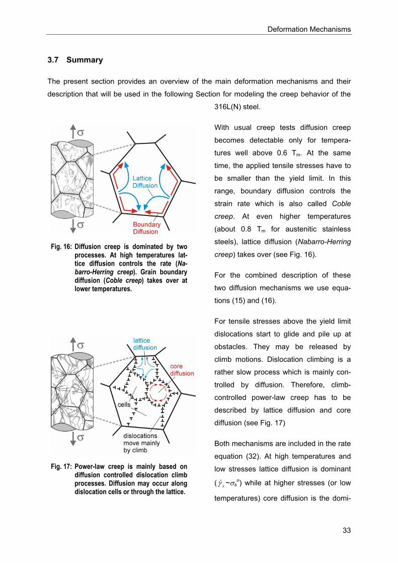
With usual creep tests diffusion creep
becomes detectable only for tempera-
tures well above 0.6 Tm. At the same
time, the applied tensile stresses have to
be smaller than the yield limit. In this
range, boundary diffusion controls the
strain rate which is also called Coble
creep. At even higher temperatures
(about 0.8 Tm for austenitic stainless
steels), lattice diffusion (Nabarro-Herring
creep) takes over (see Fig. 16).
For the combined description of these
two diffusion mechanisms we use equa-
tions (15) and (16).
For tensile stresses above the yield limit
dislocations start to glide and pile up at
obstacles. They may be released by
climb motions. Dislocation climbing is a
rather slow process which is mainly con-
trolled by diffusion. Therefore, climb-
controlled power-law creep has to be
described by lattice diffusion and core
diffusion (see Fig. 17)
Both mechanisms are included in the rate
equation (32). At high temperatures and
low stresses lattice diffusion is dominant
( sγ& ~σsn) while at higher stresses (or low
temperatures) core diffusion is the domi-
Fig. 16: Diffusion creep is dominated by two processes. At high temperatures lat-tice diffusion controls the rate (Na-barro-Herring creep). Grain boundary diffusion (Coble creep) takes over at lower temperatures.
Fig. 17: Power-law creep is mainly based on diffusion controlled dislocation climb processes. Diffusion may occur along dislocation cells or through the lattice.
Deformation Mechanisms
34
nant process ( sγ& ~σsn+2).
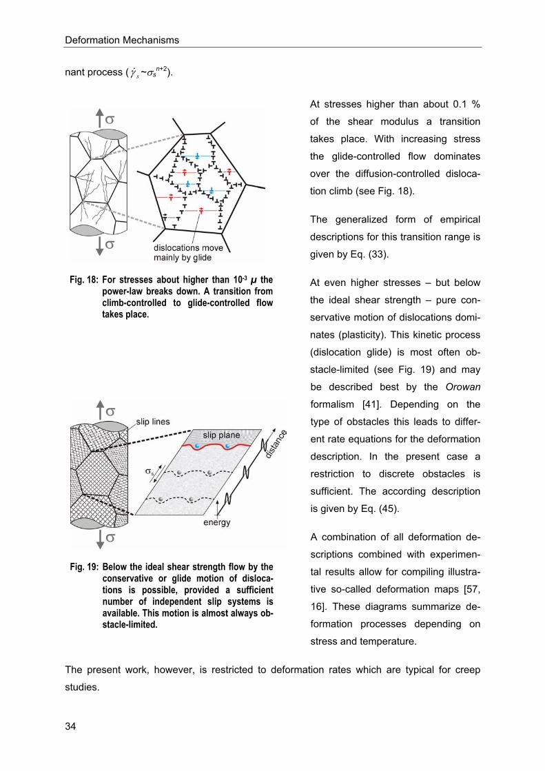
At stresses higher than about 0.1 %
of the shear modulus a transition
takes place. With increasing stress
the glide-controlled flow dominates
over the diffusion-controlled disloca-
tion climb (see Fig. 18).
The generalized form of empirical
descriptions for this transition range is
given by Eq. (33).
At even higher stresses – but below
the ideal shear strength – pure con-
servative motion of dislocations domi-
nates (plasticity). This kinetic process
(dislocation glide) is most often ob-
stacle-limited (see Fig. 19) and may
be described best by the Orowan
formalism [41]. Depending on the
type of obstacles this leads to differ-
ent rate equations for the deformation
description. In the present case a
restriction to discrete obstacles is
sufficient. The according description
is given by Eq. (45).
A combination of all deformation de-
scriptions combined with experimen-
tal results allow for compiling illustra-
tive so-called deformation maps [57,
16]. These diagrams summarize de-
formation processes depending on
stress and temperature.
The present work, however, is restricted to deformation rates which are typical for creep
studies.
Fig. 18: For stresses about higher than 10-3 µ the power-law breaks down. A transition from climb-controlled to glide-controlled flow takes place.
Fig. 19: Below the ideal shear strength flow by the conservative or glide motion of disloca-tions is possible, provided a sufficient number of independent slip systems is available. This motion is almost always ob-stacle-limited.
Steady-State Creep Model
35
4 Steady-State Creep Model
4.1 Diffusion Creep
For the description of diffusion creep we use Eqs. (15) and (16), that is
+Ω= BL
ssC D
dD
kTdπδσ
γ 2
142& , (49)
where DL and DB are lattice and boundary diffusion coefficients, respectively, with
RTQ
LL
L
eDD−
= 0 and RTQ
BB
B
eDD−
= 0 . (50)
In this model most constants are well known, like the atomic volume Ω, grain size d, and
grain boundary thickness δ (see Appendix 6.1). Values for the lattice diffusion coefficient D0L
and activation energy QL are taken from [16]. Since boundary diffusion data are not readily
available for the present
material the according val-
ues have to be adjusted to
the experiments and rea-
sonable assumptions. In
our case the boundary dif-
fusion activation energy QB
has been chosen to be 200
kJ/mol which is about 20 %
higher than the value re-
ported for 316 steels [16].
With this, the assumption
that the contributions of
lattice and boundary diffu-
sion are equal at about 0.6
TM leads to a value for D0B
of 6⋅10-6 m²/s.
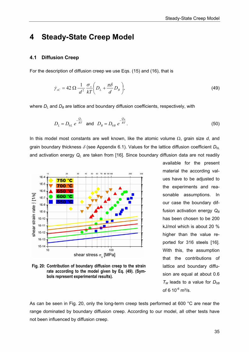
As can be seen in Fig. 20, only the long-term creep tests performed at 600 °C are near the
range dominated by boundary diffusion creep. According to our model, all other tests have
not been influenced by diffusion creep.
Fig. 20: Contribution of boundary diffusion creep to the strain rate according to the model given by Eq. (49). (Sym-bols represent experimental results).
Steady-State Creep Model
36
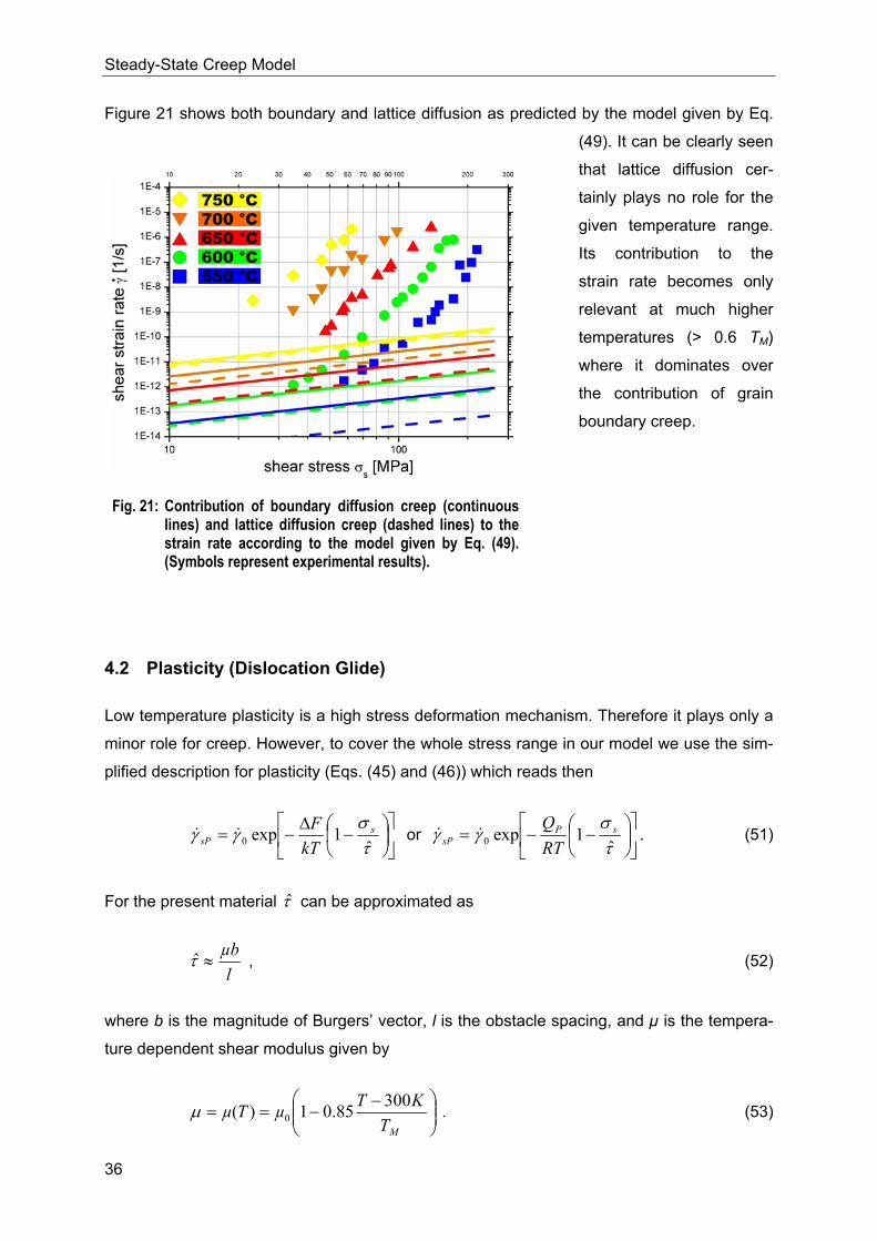
Figure 21 shows both boundary and lattice diffusion as predicted by the model given by Eq.
(49). It can be clearly seen
that lattice diffusion cer-
tainly plays no role for the
given temperature range.
Its contribution to the
strain rate becomes only
relevant at much higher
temperatures (> 0.6 TM)
where it dominates over
the contribution of grain
boundary creep.
4.2 Plasticity (Dislocation Glide)
Low temperature plasticity is a high stress deformation mechanism. Therefore it plays only a
minor role for creep. However, to cover the whole stress range in our model we use the sim-
plified description for plasticity (Eqs. (45) and (46)) which reads then
−
∆−=
τσ
γγˆ
1exp0s
sP kTF
&& or
−−=
τσ
γγˆ
1exp0sP
sP RTQ
&& . (51)
For the present material τ can be approximated as
lµb
≈τ , (52)
where b is the magnitude of Burgers’ vector, l is the obstacle spacing, and µ is the tempera-
ture dependent shear modulus given by
−−==
MTKTµTµ 30085.01)( 0µ . (53)
Fig. 21: Contribution of boundary diffusion creep (continuous lines) and lattice diffusion creep (dashed lines) to the strain rate according to the model given by Eq. (49). (Symbols represent experimental results).
Steady-State Creep Model
37
Due to the large amount of precipitates the obstacle spacing takes a relatively small value of
about 40 nm. The activation energy F∆ has been estimated to be about 0.75 µ0 b3 which
correspond to QP = 460 kJ/mol (all constants are given in Appendix 6.1).
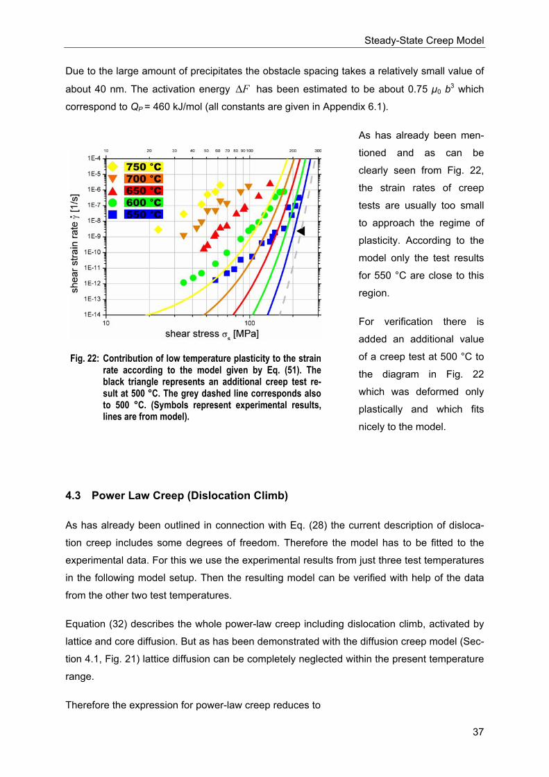
As has already been men-
tioned and as can be
clearly seen from Fig. 22,
the strain rates of creep
tests are usually too small
to approach the regime of
plasticity. According to the
model only the test results
for 550 °C are close to this
region.
For verification there is
added an additional value
of a creep test at 500 °C to
the diagram in Fig. 22
which was deformed only
plastically and which fits
nicely to the model.
4.3 Power Law Creep (Dislocation Climb)
As has already been outlined in connection with Eq. (28) the current description of disloca-
tion creep includes some degrees of freedom. Therefore the model has to be fitted to the
experimental data. For this we use the experimental results from just three test temperatures
in the following model setup. Then the resulting model can be verified with help of the data
from the other two test temperatures.
Equation (32) describes the whole power-law creep including dislocation climb, activated by
lattice and core diffusion. But as has been demonstrated with the diffusion creep model (Sec-
tion 4.1, Fig. 21) lattice diffusion can be completely neglected within the present temperature
range.
Therefore the expression for power-law creep reduces to
Fig. 22: Contribution of low temperature plasticity to the strain rate according to the model given by Eq. (51). The black triangle represents an additional creep test re-sult at 500 °C. The grey dashed line corresponds also to 500 °C. (Symbols represent experimental results, lines are from model).
Steady-State Creep Model
38
C
ns
sPL DkTbc
2
3
+
=
µσµγ& , (54)
where DC is the core diffusion coefficient with
RTQ
CC
C
eDD−
= 0 . (55)
DC is of the same order of magnitude as the grain boundary diffusion constant DB and has
therefore been chosen to be 10-5 m²/s. Again, the shear modulus µ depends on temperature
as given in Eq. (53).
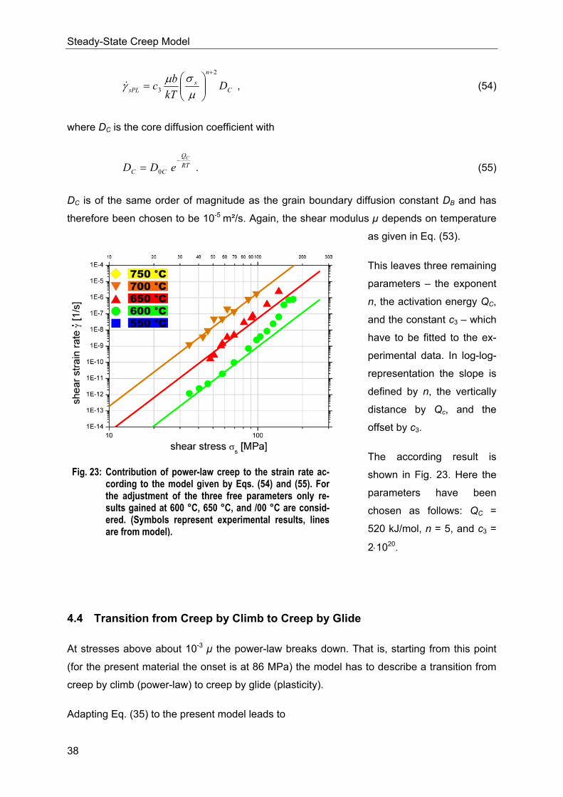
This leaves three remaining
parameters – the exponent
n, the activation energy QC,
and the constant c3 – which
have to be fitted to the ex-
perimental data. In log-log-
representation the slope is
defined by n, the vertically
distance by Qc, and the
offset by c3.
The according result is
shown in Fig. 23. Here the
parameters have been
chosen as follows: QC =
520 kJ/mol, n = 5, and c3 =
2⋅1020.
4.4 Transition from Creep by Climb to Creep by Glide
At stresses above about 10-3 µ the power-law breaks down. That is, starting from this point
(for the present material the onset is at 86 MPa) the model has to describe a transition from
creep by climb (power-law) to creep by glide (plasticity).
Adapting Eq. (35) to the present model leads to
Fig. 23: Contribution of power-law creep to the strain rate ac-cording to the model given by Eqs. (54) and (55). For the adjustment of the three free parameters only re-sults gained at 600 °C, 650 °C, and /00 °C are consid-ered. (Symbols represent experimental results, lines are from model).
Steady-State Creep Model
39
C
n
ssPLBD Dc
2
3 sinh+
′=µ
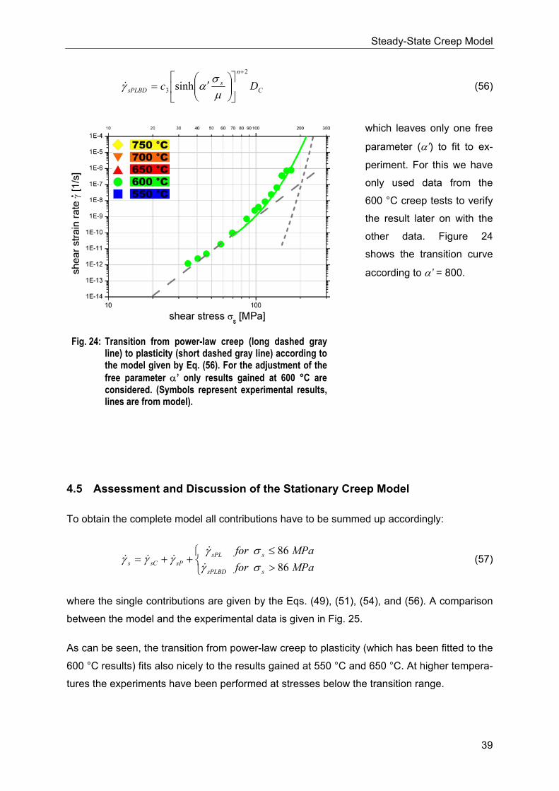
σαγ& (56)
which leaves only one free
parameter (α’) to fit to ex-
periment. For this we have
only used data from the
600 °C creep tests to verify
the result later on with the
other data. Figure 24
shows the transition curve
according to α’ = 800.
4.5 Assessment and Discussion of the Stationary Creep Model
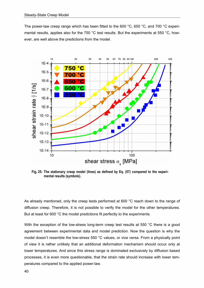
To obtain the complete model all contributions have to be summed up accordingly:
MPaforMPafor
s
s
sPLBD
sPLsPsCs 86
86>≤
++=σσ
γγ
γγγ&
&&&& (57)
where the single contributions are given by the Eqs. (49), (51), (54), and (56). A comparison
between the model and the experimental data is given in Fig. 25.
As can be seen, the transition from power-law creep to plasticity (which has been fitted to the
600 °C results) fits also nicely to the results gained at 550 °C and 650 °C. At higher tempera-
tures the experiments have been performed at stresses below the transition range.
Fig. 24: Transition from power-law creep (long dashed gray line) to plasticity (short dashed gray line) according to the model given by Eq. (56). For the adjustment of the free parameter α’ only results gained at 600 °C are considered. (Symbols represent experimental results, lines are from model).
Steady-State Creep Model
40
The power-law creep range which has been fitted to the 600 °C, 650 °C, and 700 °C experi-
mental results, applies also for the 750 °C test results. But the experiments at 550 °C, how-
ever, are well above the predictions from the model.
As already mentioned, only the creep tests performed at 600 °C reach down to the range of
diffusion creep. Therefore, it is not possible to verify the model for the other temperatures.
But at least for 600 °C the model predictions fit perfectly to the experiments.
With the exception of the low-stress long-term creep test results at 550 °C there is a good
agreement between experimental data and model prediction. Now the question is why the
model doesn’t resemble the low-stress 550 °C values, or vice versa. From a physically point
of view it is rather unlikely that an additional deformation mechanism should occur only at
lower temperatures. And since this stress range is dominated exclusively by diffusion based
processes, it is even more questionable, that the strain rate should increase with lower tem-
peratures compared to the applied power-law.
Fig. 25: The stationary creep model (lines) as defined by Eq. (57) compared to the experi-mental results (symbols).
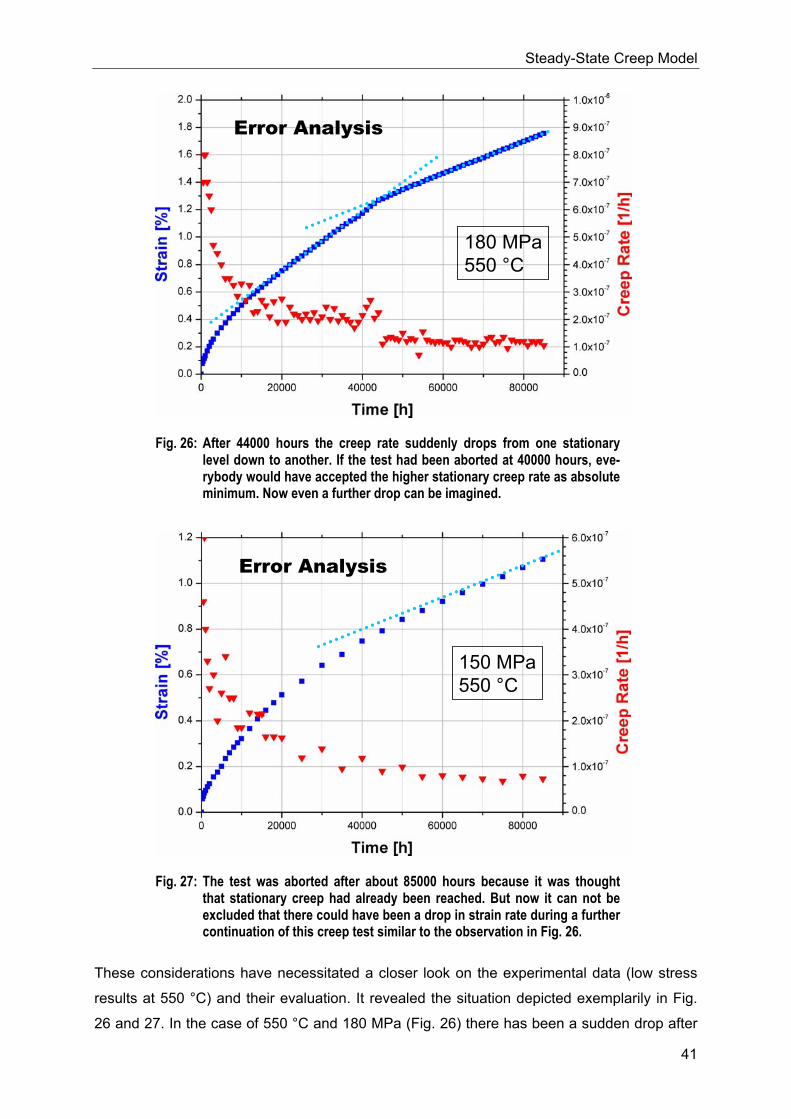
Steady-State Creep Model
41
These considerations have necessitated a closer look on the experimental data (low stress
results at 550 °C) and their evaluation. It revealed the situation depicted exemplarily in Fig.
26 and 27. In the case of 550 °C and 180 MPa (Fig. 26) there has been a sudden drop after
150 MPa550 °C
Error Analysis
Fig. 27: The test was aborted after about 85000 hours because it was thought that stationary creep had already been reached. But now it can not be excluded that there could have been a drop in strain rate during a further continuation of this creep test similar to the observation in Fig. 26.
180 MPa550 °C
Error Analysis
Fig. 26: After 44000 hours the creep rate suddenly drops from one stationary level down to another. If the test had been aborted at 40000 hours, eve-rybody would have accepted the higher stationary creep rate as absolute minimum. Now even a further drop can be imagined.
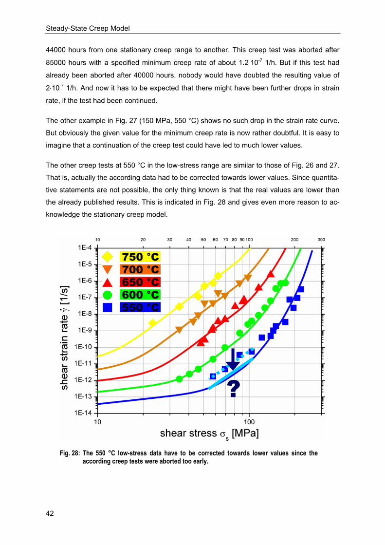
Steady-State Creep Model
42
44000 hours from one stationary creep range to another. This creep test was aborted after
85000 hours with a specified minimum creep rate of about 1.2⋅10-7 1/h. But if this test had
already been aborted after 40000 hours, nobody would have doubted the resulting value of
2⋅10-7 1/h. And now it has to be expected that there might have been further drops in strain
rate, if the test had been continued.
The other example in Fig. 27 (150 MPa, 550 °C) shows no such drop in the strain rate curve.
But obviously the given value for the minimum creep rate is now rather doubtful. It is easy to
imagine that a continuation of the creep test could have led to much lower values.
The other creep tests at 550 °C in the low-stress range are similar to those of Fig. 26 and 27.
That is, actually the according data had to be corrected towards lower values. Since quantita-
tive statements are not possible, the only thing known is that the real values are lower than
the already published results. This is indicated in Fig. 28 and gives even more reason to ac-
knowledge the stationary creep model.
?
Fig. 28: The 550 °C low-stress data have to be corrected towards lower values since the according creep tests were aborted too early.
Conclusion
43
5 Conclusion
The present investigations have been mainly based on results from creep experiments per-
formed at IMF-I, FZK with the austenitic stainless steel AISI 316 L(N) (heat no. 11477 from
Creusot-Marell). Especially long-term creep tests have shown that there is a considerable
change in the steady-state creep behavior at low stresses: the creep rates are much higher
than the values that would have been expected by an extrapolation from the usual (higher)
stress range. For component design this is a bad situation, because the real life-time would
be significantly shorter compared to estimates based on the usually available creep data.
Since AISI 316 type steel is a very common material for all kinds of applications – also for
ITER components – it would be highly helpful, if it’s seemingly odd steady-state creep behav-
ior could be described by a far reaching model. The setup of such a model was the motiva-
tion of the current paper.
At first glance, there are three possible reasons for the kink in the creep rate vs. stress curve:
(I) At very low stresses the initial strain is within the elastic range while at higher
stresses specimens are deformed plastically at the start of the creep tests. This plas-
tic deformation could act like cold working the material and, therefore, lead to higher
creep strength.
(II) Austenitic stainless steels are known for their thermal instability, that is, they are
prone to aging. Hence, more or less severe formation of precipitations could change
the microstructure significantly and cause higher creep rates, dependent on creep
time which in turn is correlated to the applied stresses.
(III) Creep rates depend on different stress-dependent deformation processes. If the
stress dependency of these processes differs considerably – let’s assume σ in one
case and σ 7 in another –, an according change of the steady-state creep rate would
be obvious.
Reason (I) can be ruled out, because the decrease in initial strain takes place continuously
with decreasing stresses. Cold work and accompanied hardening certainly plays a role in
creep behavior, but this is not an explanation for the current dramatic change in creep rate at
low stresses. Also precipitation formation can not be the reason for the observed creep be-
havior, since there is no correlation between the different precipitation types, the times of
formation and the periods of steady-state creep. Of course, precipitations may also influence
creep properties, but again, not in such a distinctive way as observed.
Conclusion
44
For a reasonable explanation this leaves only the interaction of different deformation mecha-
nisms which have been reviewed in detail: diffusional flow, power-law creep, mechanical
twinning, dislocation glide, and the elastic collapse.
It has been demonstrated that for a description of the steady-state creep behavior only grain
boundary diffusion, power-law creep, and the transition from dislocation climb to dislocation
glide are relevant, where the latter is just a limit that is barely reached with constant load
creep tests. This leads to a model consisting of three main deformation mechanisms and two
transitions:
• At very low stresses only grain boundary diffusion contributes to the strain rate which
is proportional to the stress (~ σ). This regime can only be reached by performing ex-
tremely long-term tests. In the present case diffusion creep occurred allusively after
10 years at 600 °C.
• Then there is a relatively sharp transition to creep triggered by dislocation climb. In
the present case dislocation climb depends on core diffusion and leads to creep rates
proportional to the 7th power of stress (~ σ 7) – thus the name Power-law Creep.
• Starting from medium stresses there is a continuous transition from creep by disloca-
tion climb to plasticity which depends solely on dislocation glide. The plasticity regime
is usually not reached with creep tests. Here the strain rate depends exponentially on
stress (~ eσ).
To adapt the model to creep experiments with the AISI 316 L(N) steel it needs only a few
parameters:
• grain boundary diffusion coefficient and activation energy to describe diffusion creep,
• a generic constant, the core diffusion coefficient and activation energy, and the power
exponent to describe power-law creep,
• and just a generic constant for the description of the transition from power-law creep
to plasticity.
For completeness of the model, plasticity may be described by four additional parameters.
To determine all parameters from experimental data, it needs creep tests at three different
temperatures in the usual stress range and at least some long-term experiments which reach
down into the diffusion creep regime. In the present case the latter was not quite fulfilled.
Therefore, diffusion creep might be described somewhat too conservative. However, all data
(with the exception of the 550 °C long-term experiments) fit nicely to the model predictions.
Conclusion
45
But it has been shown that these experiments were aborted too soon, that is, it was not pos-
sible to extract reliable minimum creep rates.
In summary, the presented steady-state creep model for the austenitic stainless steel AISI
316 L(N) is based on well known deformation mechanisms and can predict creep rates in the
whole temperature range relevant for application design. Due to the small number of pa-
rameters it should be no problem to apply the rate equations to other materials.
Literature
46
6 Literature
1. T. Nakazawa, Mat. Sci. Eng. A 148, 253-260 (1988).
2. M. D. Mathew, International Conference on High Nitrogen Steels, HNS 88, Lille, France, 18-20 May, 1988.
3. M. Schirra, Nucl. Eng. Design 147, 63-78 (1993)
4. M. Schirra, Nucl. Eng. Design 188, 381-384 (1999).
5. M. Schirra, KfK-Reports 4767, 4861, and 6699, Forschungszentrum Karlsruhe, Germa-ny, September 1990, August 1991, and February 2002.
6. NRIM-Creep Data Sheet No. 42-1996, National Research Institute for Metals, Tokyo, Japan.
7. M. Schirra, Annual Meeting on Nuclear Technology, Aachen, Germany, 13.-15. May 1997.
8. NRIM-Creep Data Sheet No. 14A-1982, National Research Institute for Metals, Tokyo, Japan.
9. NRIM-Creep Data Sheet No. 15A-1982, National Research Institute for Metals, Tokyo, Japan.
10. NRIM-Creep Data Sheet No. 45-1997, National Research Institute for Metals, Tokyo, Japan.
11. NRIM-Creep Data Sheet No. 6B-2000, National Research Institute for Metals, Tokyo, Japan.
12. M. Schirra, KfK-Report 4273, Forschungszentrum Karlsruhe, Germany, February 1988.
13. A. F. Padilha and P. R. Rios, ISIJ International 42, 325-337 (2002).
14. P. R. Rios and A. F. Padilha, Encyclopedia of Materials: Science and Technology, K. H. Buschow et al. (Eds.), 7836-7841, Elsevier, Amsterdam, 2001.
15. NRIM-Metallographic Atlas of Long-term Crept Materials No. M-2, National Research Institute for Metals, Tokyo, Japan, 2003.
16. H. J. Frost, and M. F. Ashby, Deformation-mechanism Maps, Pergamon Press, Oxford, 1982.
17. F. R. N. Nabarro, in: Report on Conference on Strength of Solids, Phys. Soc. of London, 75, 1948.
18. C. Herring, J. Appl. Phys. 21, 437 (1950).
19. F. Garofalo, Fundamentals of Creep and Creep-Rupture in Metals, MacMillan, New York, 1965.
20. B. Chalmers, Physical Metallurgy, John Wiley, New York, 1959.
21. A. P. Greenough, Phil. Mag. 43, 1075 (1953).
22. B. H. Alexander, M. H. Dawson, and H. P. Kling, J. Appl. Phys. 22, 439 (1951).
23. A. L. Pranatis, and G. M. Pound, Trans. AIME 203, 664 (1955).
24. A. T. Price, H. A. Hall, and A. P. Greenough, Acta Met. 12, 49 (1964).
25. E. Orowan, J. West Scot. Iron and Steel Inst. 54, 45 (1946-47).
26. W. Kauzman, Trans. AIME 143, 57 (1941).
Literature
47
27. A. H. Cottrell, and M. A. Laswon, Proc. Roy. Soc. A 19, 104 (1949).
28. P. G. Shewmon, in: Physical Metallurgy, ed. by R. W. Cahn, North-Holland Publishing Company, Amsterdam, 1965.
29. R. L. Coble, J. Appl. Phys. 34, 1679, (1963).
30. R. Raj, and M. F. Ashby, Trans. AIME 2, 1113 (1971).
31. P. Haasen, Physikalische Metallkunde, Springer-Verlag, Berlin, 1974.
32. J. Weertman, J. Mech. Phys. Solids 4, 230 (1956).
33. J. Weertman, Trans. AIME 218, 207 (1960).
34. J. Weertman, Trans. AIME 227, 1475 (1963).
35. J. Weertman, J. Appl. Phys. 26, 1213 (1955).
36. J. Weertman, J. Appl. Phys. 28, 196 and 1185 (1957).
37. O. D. Sherby, Acta Met. 10, 135 (1962).
38. D. McLean, Metallurgiacal Reviews 7, 481 (1962).
39. D. Hull, Introduction to Dislocations, 2nd Edition, Pergamon Press, Oxford, 1975.
40. J. P. Hirth, and J. Lothe, Theory of Dislocations, McGraw Hill, 1968.
41. E. Orowan, Proc. Phys. Soc. 52, 8 (1940).
42. A. S. Argon, Scripta Met. 4, 1001 (1970).
43. A. M. Brown, and M. F. Ashby, Scripta Met. 14, 1297 (1980).
44. A. K. Mukherjee, J. E. Bird, and J. E. Dorn, Trans. ASM 62, 155 ´(1969).
45. R. L. Stocker, and M. F. Ashby, Scripta Met. 7, 115 (1973).
46. S. L. Robinson, and O. D. Sherby, Acta Met. 17,109 (1969).
47. E. W. Hart, Acta Met. 5, 597 (1957).
48. R. W. Balluffi, Phys. Stat. Sol. 42, 11 (1970).
49. G. F. Bolling, and R. H. Richman, Acta Met. 13, 709 and 723 (1965).
50. A. G. Evans, and R. D. Rawlings, Phys. Stat. Sol. 34, 9 (1969).
51. U. F. Kocks, A. S. Argon, and M. F. Ashby, Prog. Mat. Sci. 19 (1975).
52. B. de Meester, C. Yin, M. Doner, and H. Conrad, in: Rate Processes in Plastic Deforma-tions, ed. by J. M. C. Li and A. K. Mukherjee, A.S.M., 1973.
53. P. Guyot, and J. E. Dorn, Can. J. Phys. 45, 983 (1967).
54. P. L. Raffo, J. Less-Common Metals 17, 133 (1969).
55. W. R. Tyson, Phil. Mag. 14, 925 (1966).
56. A. Kelly, Strong Solids, Oxford University Press, 1966.
57. M. F. Ashby, Acta Met. 20, 887 (1972).
58. L. D. Blackburn, The Generation of Isochronous Stress-Strain Curves, ASME Winter Annual Meeting, New York, 1972.
59. R. R. Vandervoort, Met. Trans. 1, 857 (1970).
60. C. M. Sellars and W. J. McG. Tegart, Mem. Sci. Rev. Met 63, 731 (1966).
61. W. A. Wong and J. J. Jonas, Trans. AIME 242, 2271 (1968).
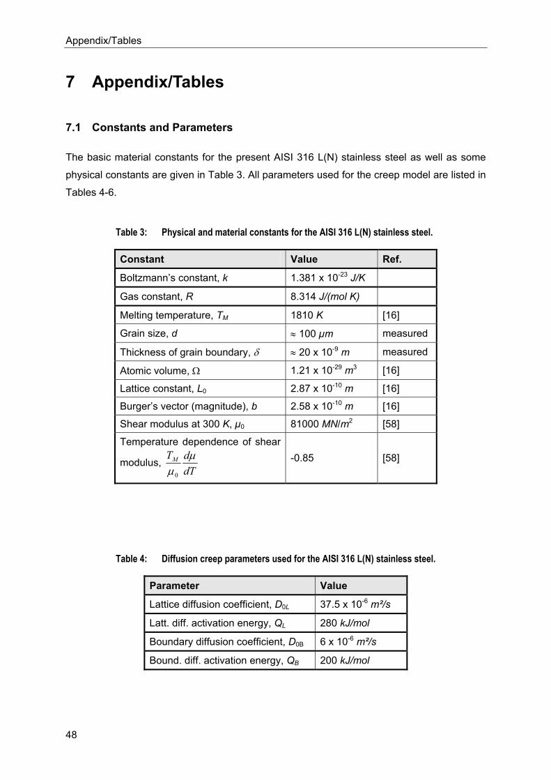
Appendix/Tables
48
7 Appendix/Tables
7.1 Constants and Parameters
The basic material constants for the present AISI 316 L(N) stainless steel as well as some
physical constants are given in Table 3. All parameters used for the creep model are listed in
Tables 4-6.
Table 3: Physical and material constants for the AISI 316 L(N) stainless steel.
Constant Value Ref.
Boltzmann’s constant, k 1.381 x 10⁻²³ J/K
Gas constant, R 8.314 J/(mol K)
Melting temperature, TM 1810 K [16]
Grain size, d ≈ 100 µm measured
Thickness of grain boundary, δ ≈ 20 x 10-9 m measured
Atomic volume, Ω 1.21 x 10⁻²⁹ m3 [16]
Lattice constant, L0 2.87 x 10⁻¹⁰ m [16]
Burger’s vector (magnitude), b 2.58 x 10⁻¹⁰ m [16]
Shear modulus at 300 K, µ0 81000 MN/m2 [58]
Temperature dependence of shear
modulus, dTdTM µ
µ0
-0.85 [58]
Table 4: Diffusion creep parameters used for the AISI 316 L(N) stainless steel.
Parameter Value
Lattice diffusion coefficient, D0L 37.5 x 10⁻⁶ m²/s
Latt. diff. activation energy, QL 280 kJ/mol
Boundary diffusion coefficient, D0B 6 x 10⁻⁶ m²/s
Bound. diff. activation energy, QB 200 kJ/mol
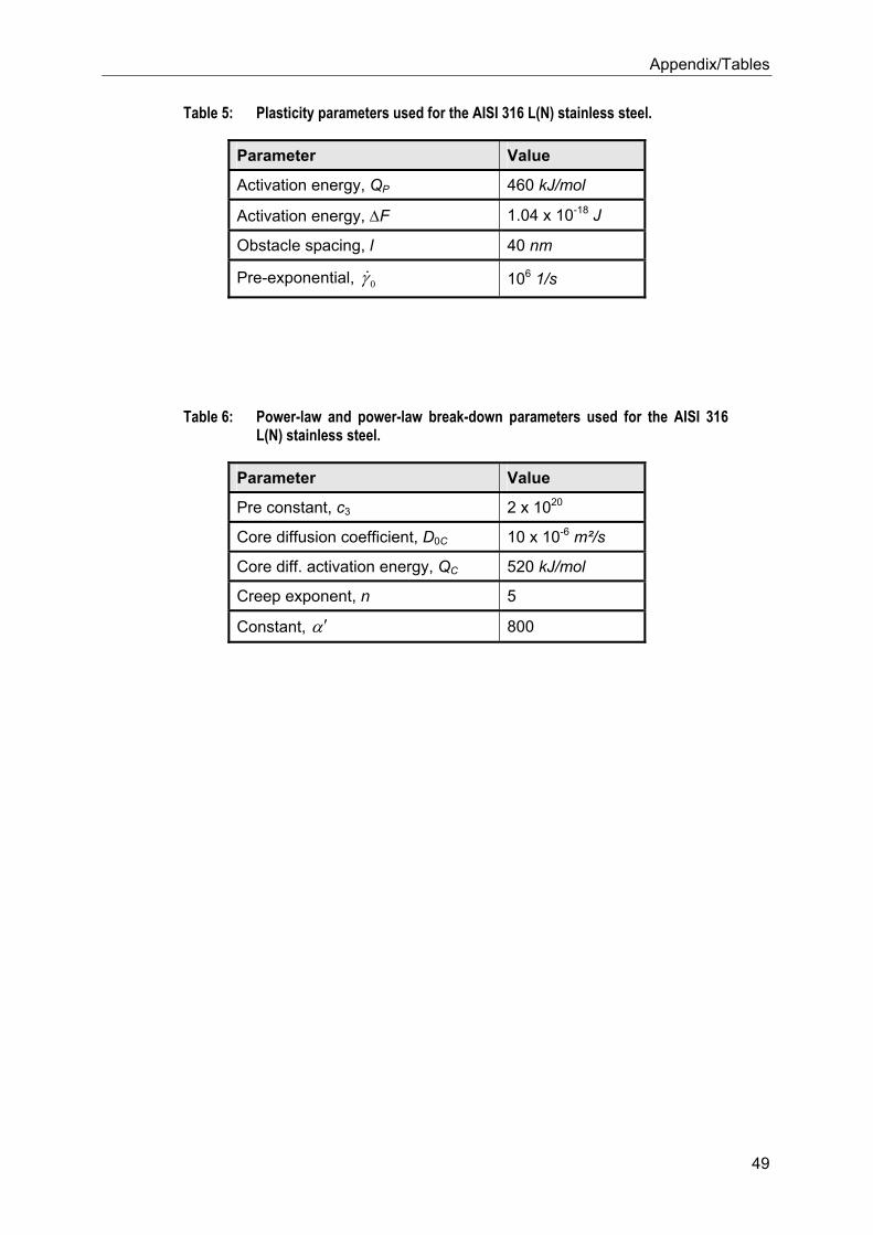
Appendix/Tables
49
Table 5: Plasticity parameters used for the AISI 316 L(N) stainless steel.
Parameter Value
Activation energy, QP 460 kJ/mol
Activation energy, ∆F 1.04 x 10⁻¹⁸ J
Obstacle spacing, l 40 nm
Pre-exponential, 0γ& 106 1/s
Table 6: Power-law and power-law break-down parameters used for the AISI 316 L(N) stainless steel.
Parameter Value
Pre constant, c3 2 x 10²⁰
Core diffusion coefficient, D0C 10 x 10-6 m²/s
Core diff. activation energy, QC 520 kJ/mol
Creep exponent, n 5
Constant, α′ 800
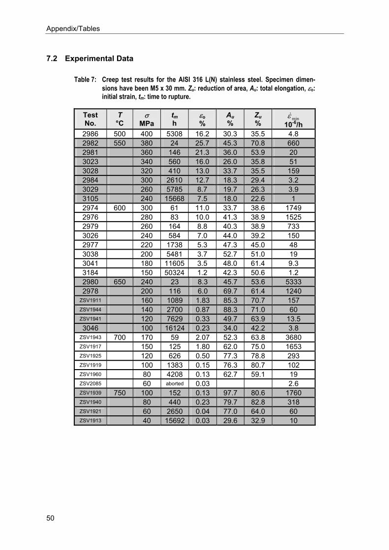
Appendix/Tables
50
7.2 Experimental Data
Table 7: Creep test results for the AISI 316 L(N) stainless steel. Specimen dimen-sions have been M5 x 30 mm. Zu: reduction of area, Au: total elongation, εo: initial strain, tm: time to rupture.
Test No.
T °C
σ MPa
tm h
εo %
Au %
Zu %
minε& 10-6/h
2986 500 400 5308 16.2 30.3 35.5 4.8 2982 550 380 24 25.7 45.3 70.8 660 2981 360 146 21.3 36.0 53.9 20 3023 340 560 16.0 26.0 35.8 51 3028 320 410 13.0 33.7 35.5 159 2984 300 2610 12.7 18.3 29.4 3.2 3029 260 5785 8.7 19.7 26.3 3.9 3105 240 15668 7.5 18.0 22.6 1 2974 600 300 61 11.0 33.7 38.6 1749 2976 280 83 10.0 41.3 38.9 1525 2979 260 164 8.8 40.3 38.9 733 3026 240 584 7.0 44.0 39.2 150 2977 220 1738 5.3 47.3 45.0 48 3038 200 5481 3.7 52.7 51.0 19 3041 180 11605 3.5 48.0 61.4 9.3 3184 150 50324 1.2 42.3 50.6 1.2 2980 650 240 23 8.3 45.7 53.6 5333 2978 200 116 6.0 69.7 61.4 1240
ZSV1911 160 1089 1.83 85.3 70.7 157 ZSV1944 140 2700 0.87 88.3 71.0 60 ZSV1941 120 7629 0.33 49.7 63.9 13.5 3046 100 16124 0.23 34.0 42.2 3.8
ZSV1943 700 170 59 2.07 52.3 63.8 3680 ZSV1917 150 125 1.80 62.0 75.0 1653 ZSV1925 120 626 0.50 77.3 78.8 293 ZSV1919 100 1383 0.15 76.3 80.7 102 ZSV1960 80 4208 0.13 62.7 59.1 19 ZSV2085 60 aborted 0.03 2.6 ZSV1939 750 100 152 0.13 97.7 80.6 1760 ZSV1940 80 440 0.23 79.7 82.8 318 ZSV1921 60 2650 0.04 77.0 64.0 60 ZSV1913 40 15692 0.03 29.6 32.9 10
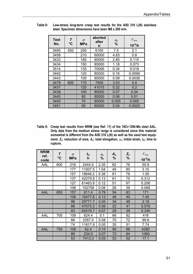
Appendix/Tables
51
Table 8: Low-stress long-term creep test results for the AISI 316 L(N) stainless steel. Specimen dimensions have been M8 x 200 mm.
Test No.
T °C
σ MPa
aborted after
h εo %
minε&
10-6/h 3495 550 250 6100 7.5 2.1 3458 210 60000 4.83 0.8 3433 180 85000 2.85 0.115 3434 150 85000 1.18 0.073 3514 135 70006 0.34 0.018 3442 120 85000 0.16 0.0099 3443 100 85000 0.09 0.0036 3478 600 170 7500 3.03 5.0 3437 120 41015 0.32 0.2 3438 100 85000 0.07 0.04 3445 80 85000 0.06 0.01 3450 70 85000 0.055 0.005 3451 60 85000 0.04 0.0025
Table 9: Creep test results from NRIM (see Ref. 11) of the 18Cr-12Ni-Mo steel AAL. Only data from the medium stress range is considered since this material somewhat is different from the AISI 316 L(N) as well as the used test equip-ment. Zu: reduction of area, Au: total elongation, εo: initial strain, tm: time to rupture.
NRIM ref.
code T °C
σ MPa
tm h
εo %
Au %
Zu %
minε&
10-6/h AAL 600 216 2444.5 2.35 62 76 50.9
177 11007.5 1.04 49 80 3.10 157 19646.2 0.38 61 78 1.05 137 42079.8 0.13 61 75 0.312 127 61463.9 0.12 51 67 0.208 108 152758 0.08 26 39 0.068
AAL 650 157 811.4 0.78 54 83 171 108 10477.6 0.13 46 40 7.45 98 25771.7 0.05 34 48 2.18 88 47073.3 0.06 22 41 0.576 83 64516.7 0.07 29 39 0.346
AAL 700 108 624.4 0.1 66 82 416 88 2357.0 0.08 70 72 99.8 74 11817.9 0.05 35 51 7.74
AAL 750 108 62.4 0.15 90 86 4280 88 234.0 0.07 72 84 1060 53 7413.3 0.05 53 52 17.1
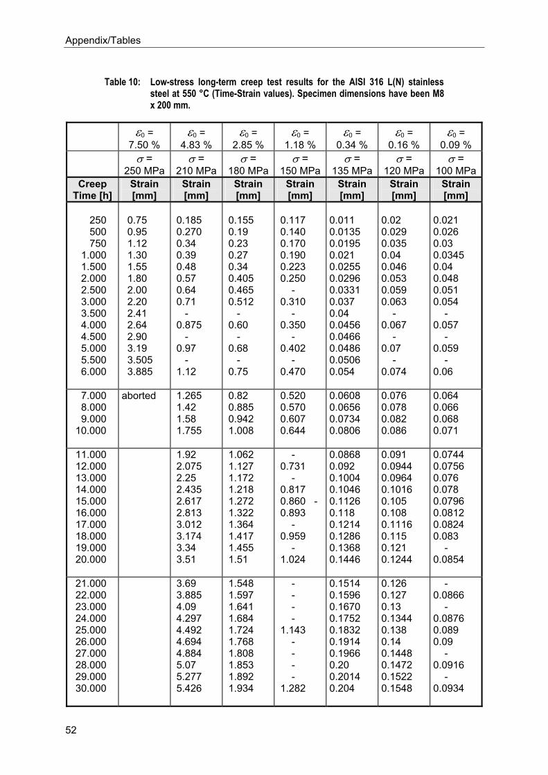
Appendix/Tables
52
Table 10: Low-stress long-term creep test results for the AISI 316 L(N) stainless steel at 550 °C (Time-Strain values). Specimen dimensions have been M8 x 200 mm.
ε0 = 7.50 %
ε0 = 4.83 %
ε0 = 2.85 %
ε0 = 1.18 %
ε0 = 0.34 %
ε0 = 0.16 %
ε0 = 0.09 %
σ = 250 MPa
σ = 210 MPa
σ = 180 MPa
σ = 150 MPa
σ = 135 MPa
σ = 120 MPa
σ = 100 MPa
Creep Time [h]
Strain [mm]
Strain [mm]
Strain [mm]
Strain [mm]
Strain [mm]
Strain [mm]
Strain [mm]
250 500 750 1.000 1.500 2.000 2.500 3.000 3.500 4.000 4.500 5.000 5.500 6.000
0.75 0.95 1.12 1.30 1.55 1.80 2.00 2.20 2.41 2.64 2.90 3.19 3.505 3.885
0.185 0.270 0.34 0.39 0.48 0.57 0.64 0.71 - 0.875 - 0.97 - 1.12
0.155 0.19 0.23 0.27 0.34 0.405 0.465 0.512 - 0.60 - 0.68 - 0.75
0.117 0.140 0.170 0.190 0.223 0.250 - 0.310 - 0.350 - 0.402 - 0.470
0.011 0.0135 0.0195 0.021 0.0255 0.0296 0.0331 0.037 0.04 0.0456 0.0466 0.0486 0.0506 0.054
0.02 0.029 0.035 0.04 0.046 0.053 0.059 0.063 - 0.067 - 0.07 - 0.074
0.021 0.026 0.03 0.0345 0.04 0.048 0.051 0.054 - 0.057 - 0.059 - 0.06
7.000 8.000 9.000 10.000
aborted
1.265 1.42 1.58 1.755
0.82 0.885 0.942 1.008
0.520 0.570 0.607 0.644
0.0608 0.0656 0.0734 0.0806
0.076 0.078 0.082 0.086
0.064 0.066 0.068 0.071
11.000 12.000 13.000 14.000 15.000 16.000 17.000 18.000 19.000 20.000
1.92 2.075 2.25 2.435 2.617 2.813 3.012 3.174 3.34 3.51
1.062 1.127 1.172 1.218 1.272 1.322 1.364 1.417 1.455 1.51
- 0.731 - 0.817 0.860 - 0.893 - 0.959 - 1.024
0.0868 0.092 0.1004 0.1046 0.1126 0.118 0.1214 0.1286 0.1368 0.1446
0.091 0.0944 0.0964 0.1016 0.105 0.108 0.1116 0.115 0.121 0.1244
0.0744 0.0756 0.076 0.078 0.0796 0.0812 0.0824 0.083 - 0.0854
21.000 22.000 23.000 24.000 25.000 26.000 27.000 28.000 29.000 30.000
3.69 3.885 4.09 4.297 4.492 4.694 4.884 5.07 5.277 5.426
1.548 1.597 1.641 1.684 1.724 1.768 1.808 1.853 1.892 1.934
- - - - 1.143 - - - - 1.282
0.1514 0.1596 0.1670 0.1752 0.1832 0.1914 0.1966 0.20 0.2014 0.204
0.126 0.127 0.13 0.1344 0.138 0.14 0.1448 0.1472 0.1522 0.1548
- 0.0866 - 0.0876 0.089 0.09 - 0.0916 - 0.0934
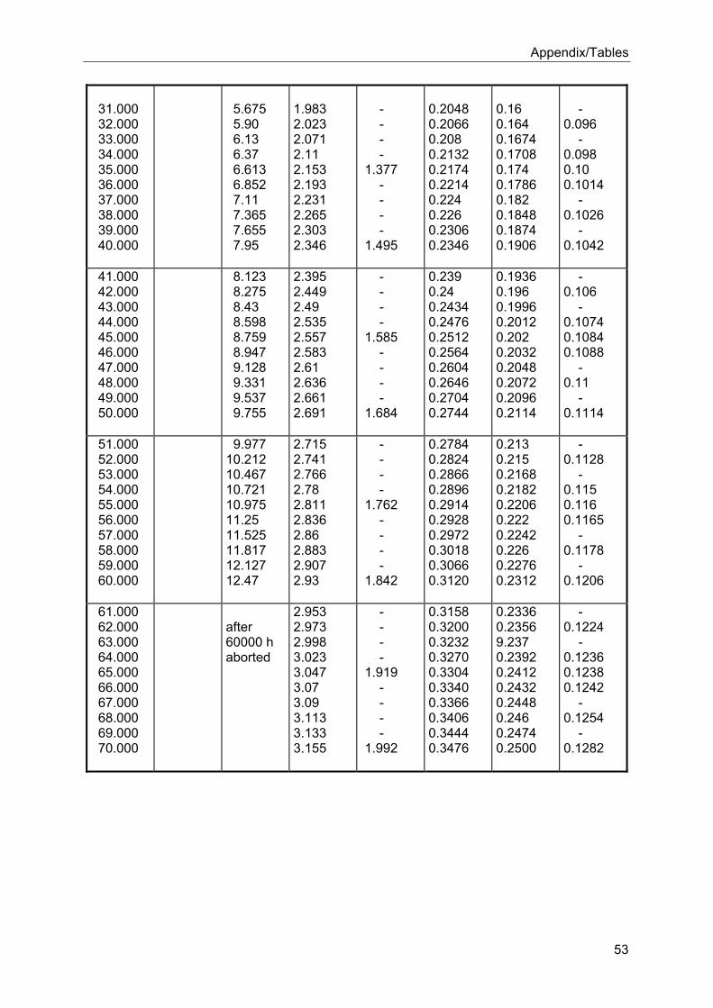
Appendix/Tables
53
31.000 32.000 33.000 34.000 35.000 36.000 37.000 38.000 39.000 40.000
5.675 5.90 6.13 6.37 6.613 6.852 7.11 7.365 7.655 7.95
1.983 2.023 2.071 2.11 2.153 2.193 2.231 2.265 2.303 2.346
- - - - 1.377 - - - - 1.495
0.2048 0.2066 0.208 0.2132 0.2174 0.2214 0.224 0.226 0.2306 0.2346
0.16 0.164 0.1674 0.1708 0.174 0.1786 0.182 0.1848 0.1874 0.1906
- 0.096 - 0.098 0.10 0.1014 - 0.1026 - 0.1042
41.000 42.000 43.000 44.000 45.000 46.000 47.000 48.000 49.000 50.000
8.123 8.275 8.43 8.598 8.759 8.947 9.128 9.331 9.537 9.755
2.395 2.449 2.49 2.535 2.557 2.583 2.61 2.636 2.661 2.691
- - - - 1.585 - - - - 1.684
0.239 0.24 0.2434 0.2476 0.2512 0.2564 0.2604 0.2646 0.2704 0.2744
0.1936 0.196 0.1996 0.2012 0.202 0.2032 0.2048 0.2072 0.2096 0.2114
- 0.106 - 0.1074 0.1084 0.1088 - 0.11 - 0.1114
51.000 52.000 53.000 54.000 55.000 56.000 57.000 58.000 59.000 60.000
9.977 10.212 10.467 10.721 10.975 11.25 11.525 11.817 12.127 12.47
2.715 2.741 2.766 2.78 2.811 2.836 2.86 2.883 2.907 2.93
- - - - 1.762 - - - - 1.842
0.2784 0.2824 0.2866 0.2896 0.2914 0.2928 0.2972 0.3018 0.3066 0.3120
0.213 0.215 0.2168 0.2182 0.2206 0.222 0.2242 0.226 0.2276 0.2312
- 0.1128 - 0.115 0.116 0.1165 - 0.1178 - 0.1206
61.000 62.000 63.000 64.000 65.000 66.000 67.000 68.000 69.000 70.000
after 60000 h aborted
2.953 2.973 2.998 3.023 3.047 3.07 3.09 3.113 3.133 3.155
- - - - 1.919 - - - - 1.992
0.3158 0.3200 0.3232 0.3270 0.3304 0.3340 0.3366 0.3406 0.3444 0.3476
0.2336 0.2356 9.237 0.2392 0.2412 0.2432 0.2448 0.246 0.2474 0.2500
- 0.1224 - 0.1236 0.1238 0.1242 - 0.1254 - 0.1282
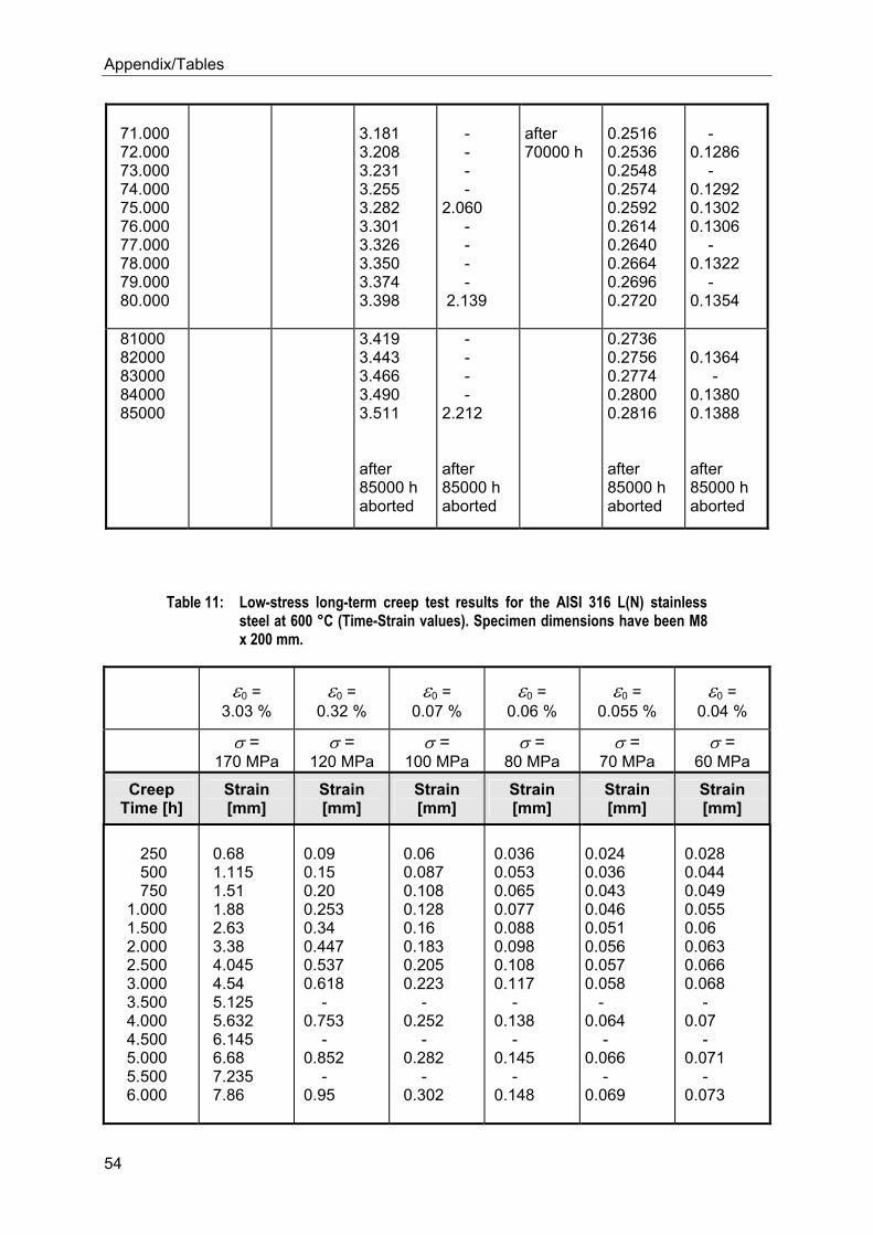
Appendix/Tables
54
71.000 72.000 73.000 74.000 75.000 76.000 77.000 78.000 79.000 80.000
3.181 3.208 3.231 3.255 3.282 3.301 3.326 3.350 3.374 3.398
- - - - 2.060 - - - - 2.139
after 70000 h
0.2516 0.2536 0.2548 0.2574 0.2592 0.2614 0.2640 0.2664 0.2696 0.2720
- 0.1286 - 0.1292 0.1302 0.1306 - 0.1322 - 0.1354
81000 82000 83000 84000 85000
3.419 3.443 3.466 3.490 3.511 after 85000 h aborted
- - - - 2.212 after 85000 h aborted
0.2736 0.2756 0.2774 0.2800 0.2816 after 85000 h aborted
0.1364 - 0.1380 0.1388 after 85000 h aborted
Table 11: Low-stress long-term creep test results for the AISI 316 L(N) stainless steel at 600 °C (Time-Strain values). Specimen dimensions have been M8 x 200 mm.
ε0 = 3.03 %
ε0 = 0.32 %
ε0 = 0.07 %
ε0 = 0.06 %
ε0 = 0.055 %
ε0 = 0.04 %
σ = 170 MPa
σ = 120 MPa
σ = 100 MPa
σ = 80 MPa
σ = 70 MPa
σ = 60 MPa
Creep Time [h]
Strain [mm]
Strain [mm]
Strain [mm]
Strain [mm]
Strain [mm]
Strain [mm]
250 500 750 1.000 1.500 2.000 2.500 3.000 3.500 4.000 4.500 5.000 5.500 6.000
0.68 1.115 1.51 1.88 2.63 3.38 4.045 4.54 5.125 5.632 6.145 6.68 7.235 7.86
0.09 0.15 0.20 0.253 0.34 0.447 0.537 0.618 - 0.753 - 0.852 - 0.95
0.06 0.087 0.108 0.128 0.16 0.183 0.205 0.223 - 0.252 - 0.282 - 0.302
0.036 0.053 0.065 0.077 0.088 0.098 0.108 0.117 - 0.138 - 0.145 - 0.148
0.024 0.036 0.043 0.046 0.051 0.056 0.057 0.058 - 0.064 - 0.066 - 0.069
0.028 0.044 0.049 0.055 0.06 0.063 0.066 0.068 - 0.07 - 0.071 - 0.073
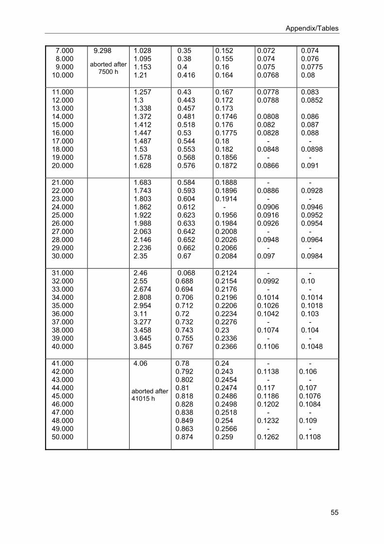
Appendix/Tables
55
7.000 8.000 9.000 10.000
9.298 aborted after
7500 h
1.028 1.095 1.153 1.21
0.35 0.38 0.4 0.416
0.152 0.155 0.16 0.164
0.072 0.074 0.075 0.0768
0.074 0.076 0.0775 0.08
11.000 12.000 13.000 14.000 15.000 16.000 17.000 18.000 19.000 20.000
1.257 1.3 1.338 1.372 1.412 1.447 1.487 1.53 1.578 1.628
0.43 0.443 0.457 0.481 0.518 0.53 0.544 0.553 0.568 0.576
0.167 0.172 0.173 0.1746 0.176 0.1775 0.18 0.182 0.1856 0.1872
0.0778 0.0788 0.0808 0.082 0.0828 - 0.0848 - 0.0866
0.083 0.0852 0.086 0.087 0.088 - 0.0898 - 0.091
21.000 22.000 23.000 24.000 25.000 26.000 27.000 28.000 29.000 30.000
1.683 1.743 1.803 1.862 1.922 1.988 2.063 2.146 2.236 2.35
0.584 0.593 0.604 0.612 0.623 0.633 0.642 0.652 0.662 0.67
0.1888 0.1896 0.1914 - 0.1956 0.1984 0.2008 0.2026 0.2066 0.2084
- 0.0886 - 0.0906 0.0916 0.0926 - 0.0948 - 0.097
- 0.0928 - 0.0946 0.0952 0.0954 - 0.0964 - 0.0984
31.000 32.000 33.000 34.000 35.000 36.000 37.000 38.000 39.000 40.000
2.46 2.55 2.674 2.808 2.954 3.11 3.277 3.458 3.645 3.845
0.068 0.688 0.694 0.706 0.712 0.72 0.732 0.743 0.755 0.767
0.2124 0.2154 0.2176 0.2196 0.2206 0.2234 0.2276 0.23 0.2336 0.2366
- 0.0992 - 0.1014 0.1026 0.1042 - 0.1074 - 0.1106
- 0.10 - 0.1014 0.1018 0.103 - 0.104 - 0.1048
41.000 42.000 43.000 44.000 45.000 46.000 47.000 48.000 49.000 50.000
4.06 aborted after41015 h
0.78 0.792 0.802 0.81 0.818 0.828 0.838 0.849 0.863 0.874
0.24 0.243 0.2454 0.2474 0.2486 0.2498 0.2518 0.254 0.2566 0.259
- 0.1138 - 0.117 0.1186 0.1202 - 0.1232 - 0.1262
- 0.106 - 0.107 0.1076 0.1084 - 0.109 - 0.1108
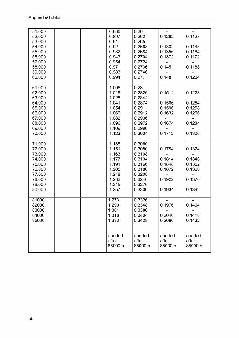
Appendix/Tables
56
51.000 52.000 53.000 54.000 55.000 56.000 57.000 58.000 59.000 60.000
0.886 0.897 0.91 0.92 0.932 0.943 0.954 0.97 0.983 0.994
0.26 0.262 0.265 0.2668 0.2684 0.2704 0.2724 0.2736 0.2746 0.277
- 0.1292 - 0.1332 0.1356 0.1372 - 0.145 - 0.148
- 0.1128 - 0.1148 0.1164 0.1172 - 0.1188 - 0.1204
61.000 62.000 63.000 64.000 65.000 66.000 67.000 68.000 69.000 70.000
1.006 1.016 1.028 1.041 1.054 1.066 1.082 1.096 1.109 1.123
0.28 0.2826 0.2844 0.2874 0.29 0.2912 0.2936 0.2972 0.2996 0.3034
- 0.1512 - 0.1566 0.1596 0.1632 - 0.1674 - 0.1712
- 0.1228 - 0.1254 0.1258 0.1266 - 0.1284 - 0.1306
71.000 72.000 73.000 74.000 75.000 76.000 77.000 78.000 79.000 80.000
1.138 1.151 1.163 1.177 1.191 1.205 1.218 1.232 1.245 1.257
0.3060 0.3080 0.3108 0.3134 0.3166 0.3180 0.3208 0.3246 0.3276 0.3306
- 0.1754 - 0.1814 0.1848 0.1872 - 0.1922 - 0.1934
- 0.1324 - 0.1346 0.1352 0.1360 - 0.1376 - 0.1392
81000 82000 83000 84000 85000
1.273 1.290 1.304 1.318 1.333 aborted after 85000 h
0.3326 0.3348 0.3386 0.3404 0.3428 aborted after 85000 h
- 0.1976 - 0.2046 0.2066 aborted after 85000 h
- 0.1404 - 0.1418 0.1432 aborted after 85000 h
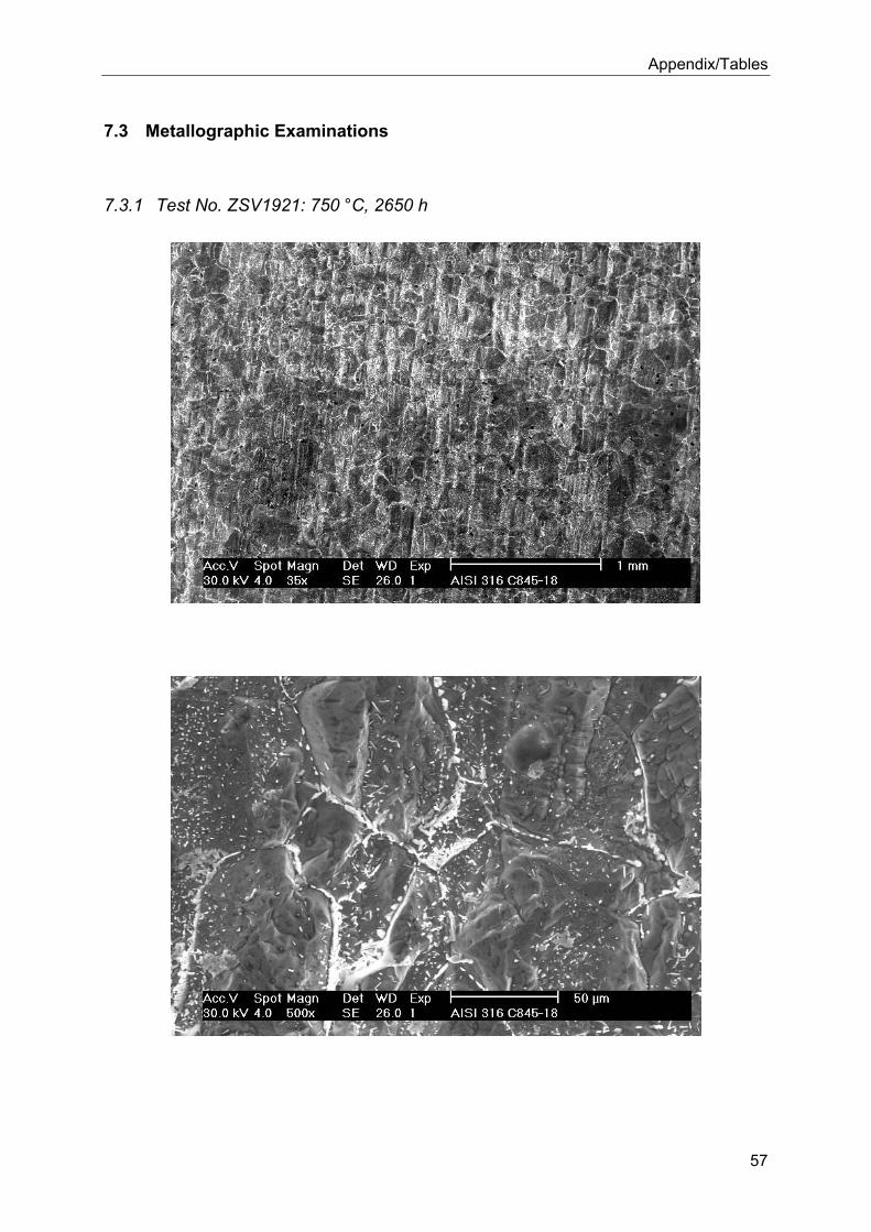
Appendix/Tables
57
7.3 Metallographic Examinations
7.3.1 Test No. ZSV1921: 750 °C, 2650 h
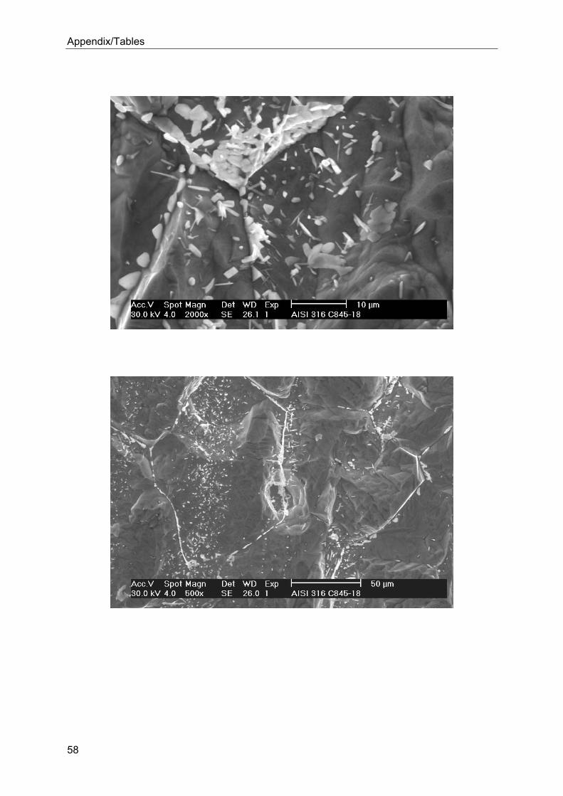
Appendix/Tables
58
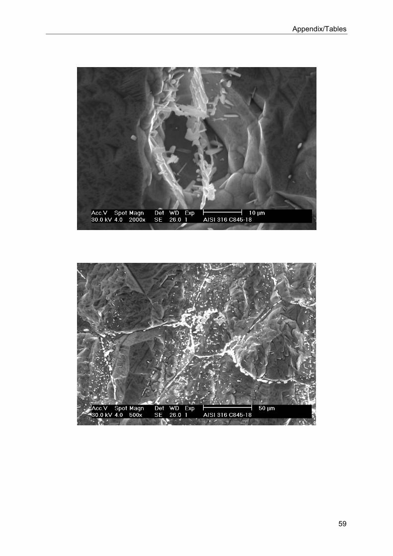
Appendix/Tables
59
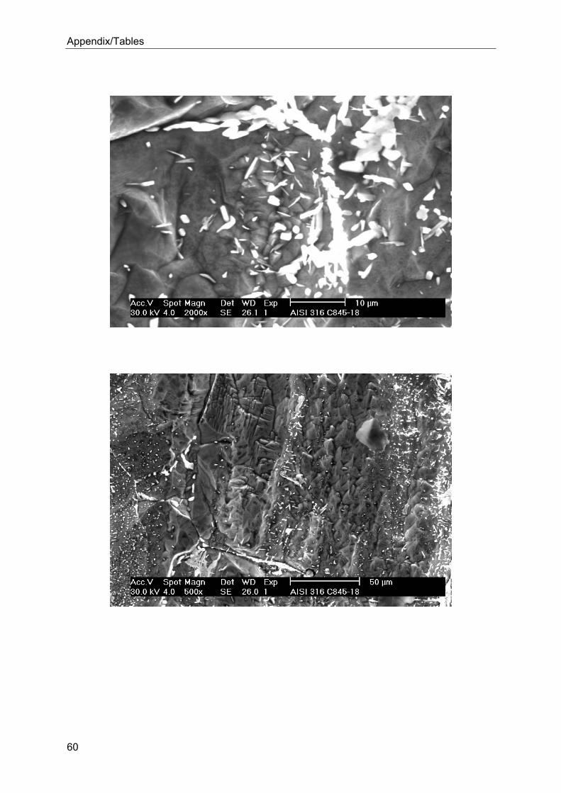
Appendix/Tables
60
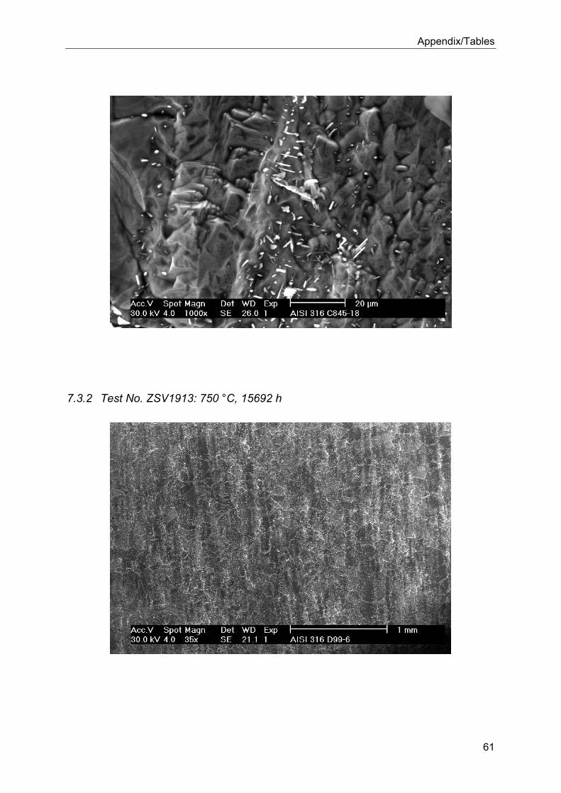
Appendix/Tables
61
7.3.2 Test No. ZSV1913: 750 °C, 15692 h
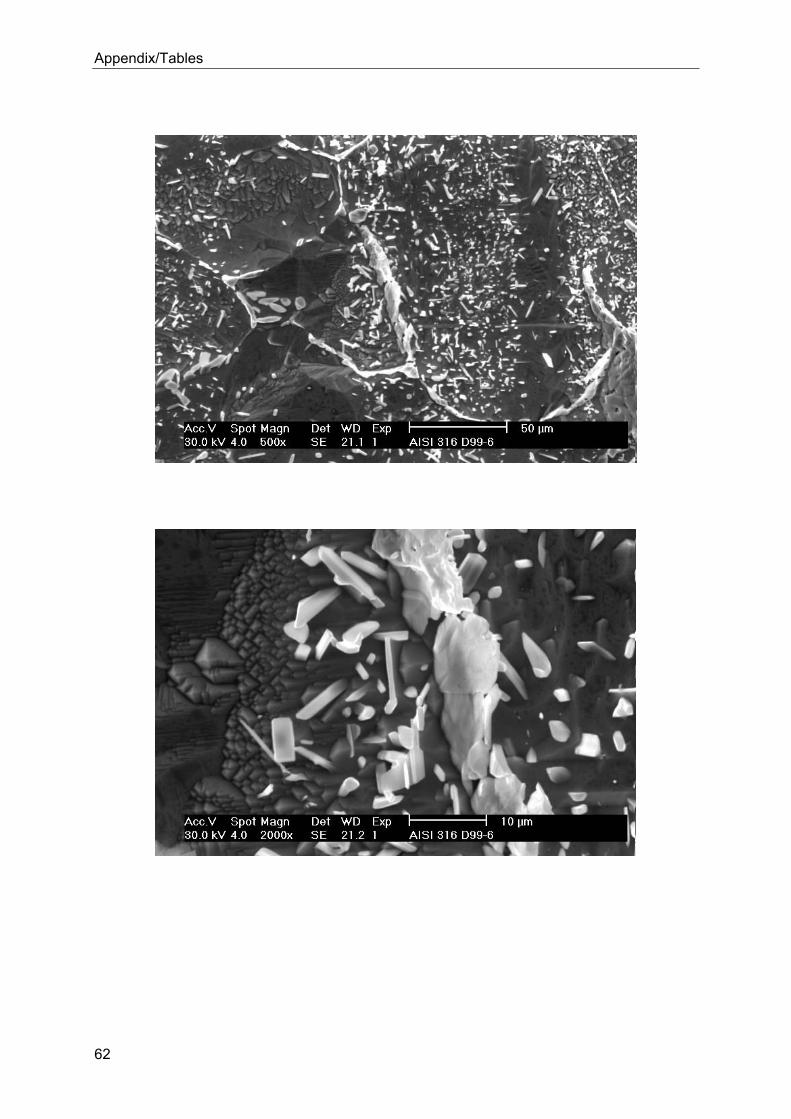
Appendix/Tables
62
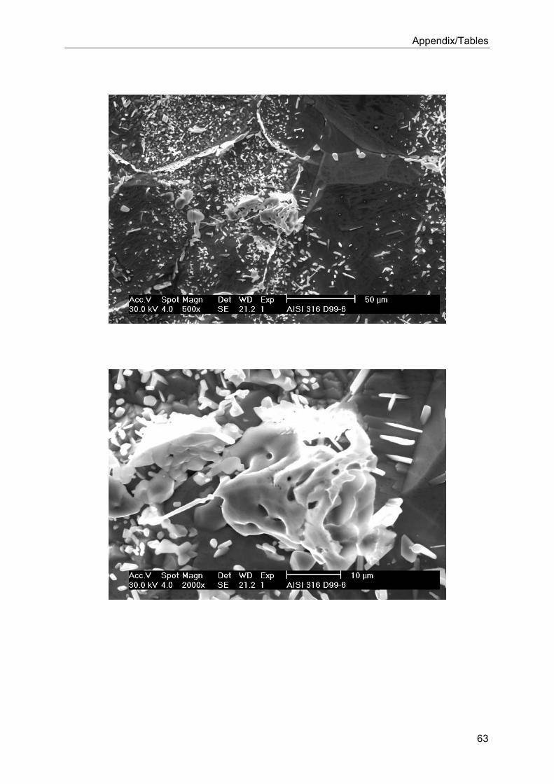
Appendix/Tables
63
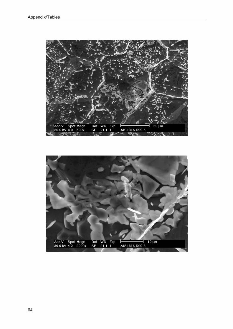
Appendix/Tables
64
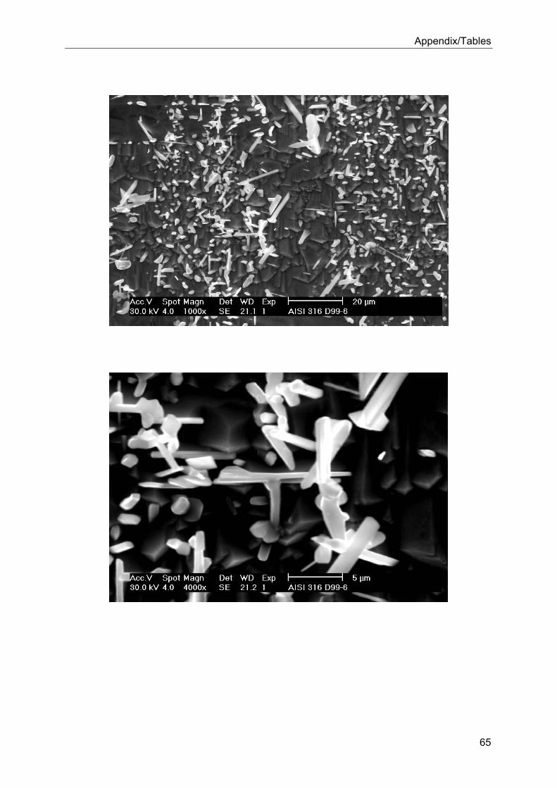
Appendix/Tables
65
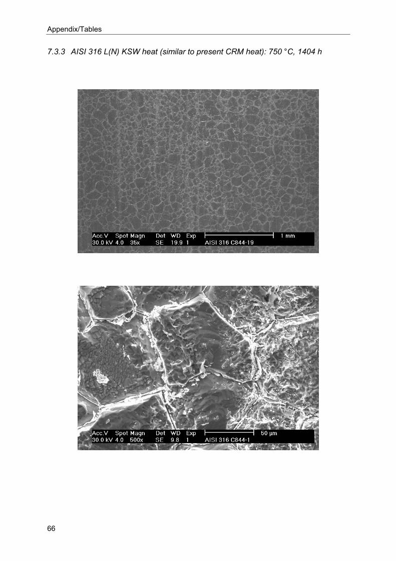
Appendix/Tables
66
7.3.3 AISI 316 L(N) KSW heat (similar to present CRM heat): 750 °C, 1404 h
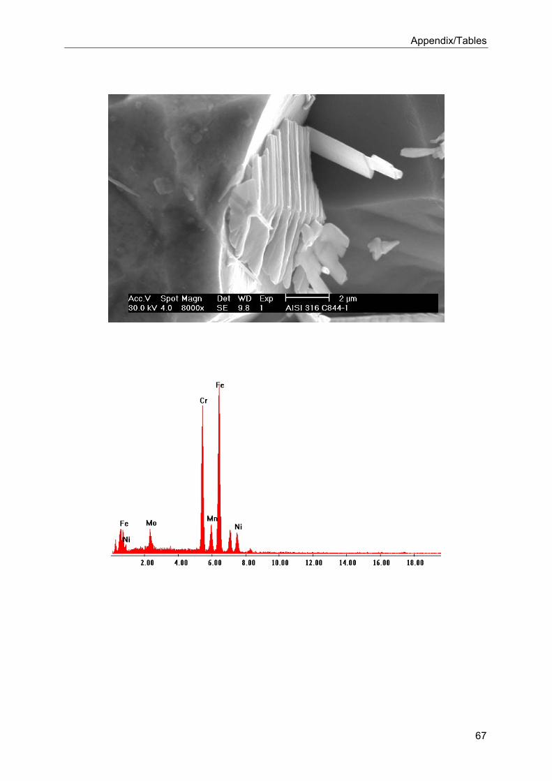
Appendix/Tables
67
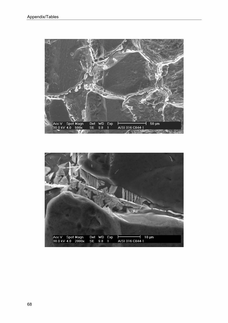
Appendix/Tables
68
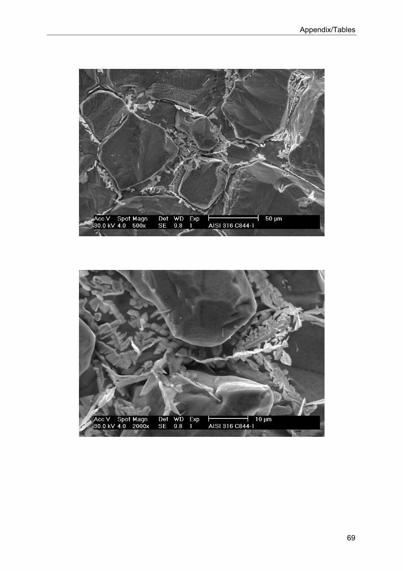
Appendix/Tables
69
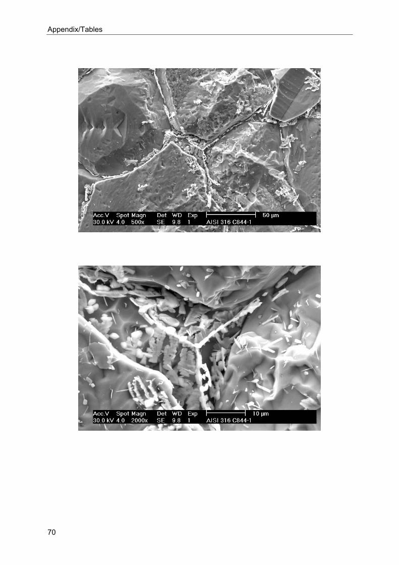
Appendix/Tables
70
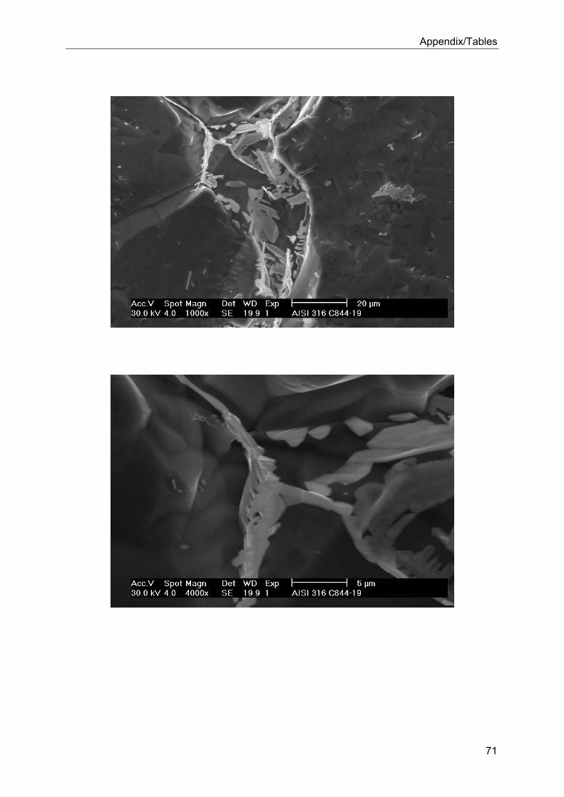
Appendix/Tables
71
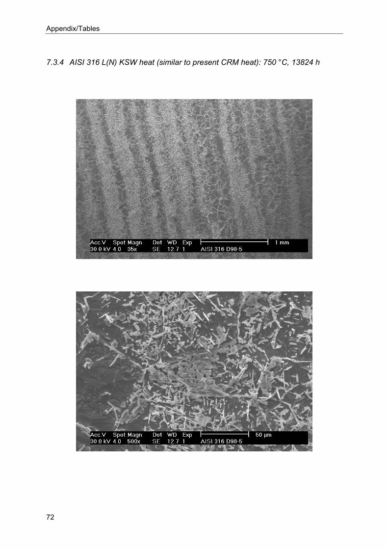
Appendix/Tables
72
7.3.4 AISI 316 L(N) KSW heat (similar to present CRM heat): 750 °C, 13824 h
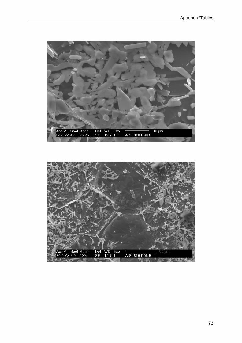
Appendix/Tables
73
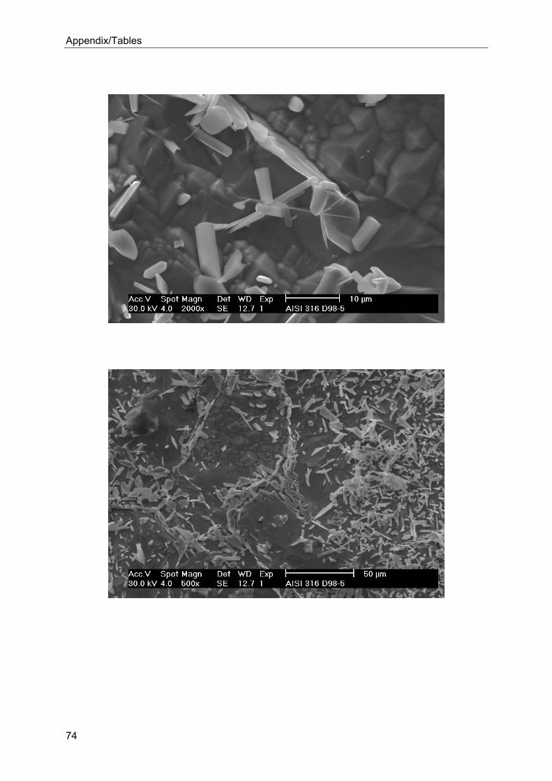
Appendix/Tables
74
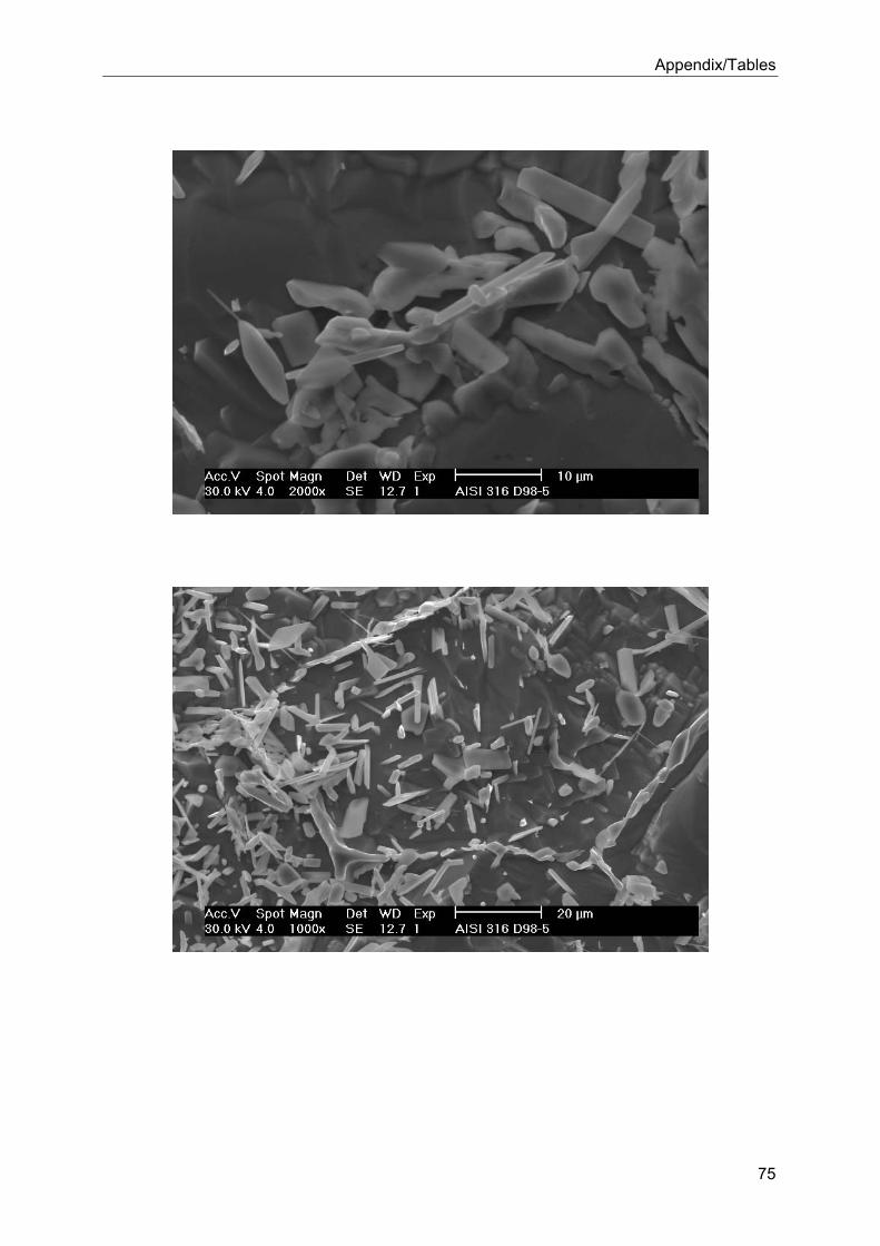
Appendix/Tables
75
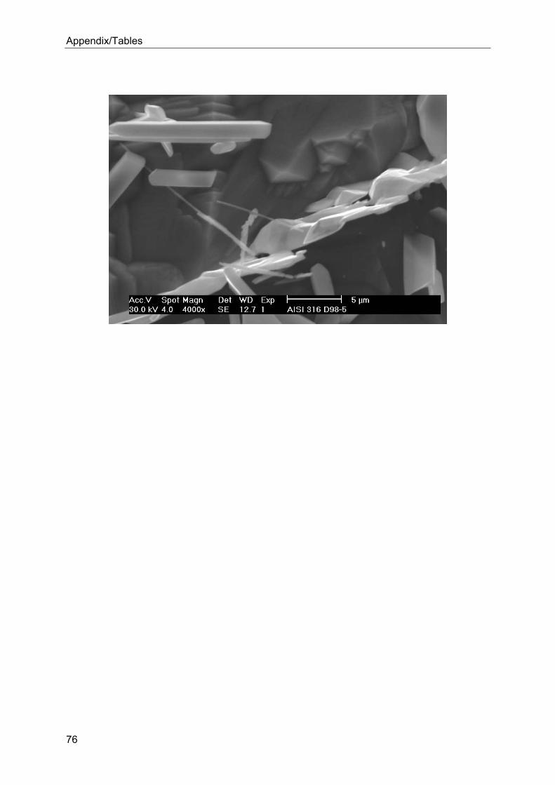
Appendix/Tables
76