1 Davies

Data Analysis and Modeling for PDE

Process Planning and Control

by: Charles Justin Davies

ISE 677

Professor: Dr. Thom Hodgson

North Carolina State University

2 Davies

Tables of Contents

Abstract……………………………………………………………………………3

Introduction………………………………………………………………………..4

Phase 1……………………………………………………………………………4

Phase 2…………………………………………………………………………..11

Phase 3…………………………………………………………………………..14

The Next Step….Where the Research Goes Now………………………….19

Conclusion……………………………………………………………………….20

3 Davies

Abstract

In any manufacturing environment, production planning and control is essential in order for

companies to remain competitive. There is a strong emphasis on this factor of operations in

manufacturing. Such an emphasis is needed in the General Electric Energy Division Product

Definition Engineering Department. Visual flow network techniques were utilized to test a

sample of data which revealed measurable results. These results suggested repeated instances of

rework loops, work stalls due to scope change, and errors from standard practices. An

opportunity for improvement was highlighted based upon these findings. The researcher

understood that improvements are based upon a medium of measurement which sets a baseline

of current state. Efforts were engaged to develop the current state for numerous activities within

the PDE organization. Simple averages were employed for this reflection. The data was first

extracted from Activity Management Tools generated by individual drafters who performed the

work. The results of the data did not fit intuition of the respective management and employees

involved. Thus, the AMT was decommissioned as a tool to capture the current state. Data

analysis was applied to a database that houses durations of activities based upon the time sheet

recording database. The data of drafting activities for any given duration from this approach was

considerably skewed. Measures of central tendency and spread were applied. These results

proved insufficient for activity planning. All of the data researched possessed skewed

distributions with considerable spreads. Due to this spread, graphical representations of the data

suggested variations that would make accurate planning impossible. A normalization method

was applied to capture a measurement mechanism based upon confidence intervals. Such a

method proved valuable in acquiring a baseline for measurement and a gage for planning and

loading of drafting work.

4 Davies

Introduction

Today’s business environment requires that companies become more competitive by

reducing costs. This concept has traditionally been applied to the manufacturing environment

where cycle times, lead times, WIP status etc. define the financial measuring stick of the

organization. Nonetheless, there is extreme value in applying these approaches to the other

industries.

There has been a need to quantitatively measure the operational health of the Product

Definition Engineering Division of the General Electric Energy Division. Although there is no

production per say on a manufacturing line, this organization provides design services for the gas

turbine energy division. Currently, the department has little visibility to the loading within the

various groups along with any metrics from which to be measured such as productivity. As a

contractor for GE, QuEST Global Services approached this need as an opportunity to partner

with GE to make them more productive and efficient.

The purpose of this paper is to methodically demonstrate the problem solving approach

that was implemented to meet the end goal – defined metrics for drafting activities. This paper

will also demonstrate methods used to convince management that the approaches developed

were optimal based on the current research performed and the resources available. It is important

to understand that 90% of the problem solving is communicating to upper management and all

employees involved. The method of communication and the approach of the communication are

key factors.

Phase 1

Determining the current state of the drafting system was the first step in defining

appropriate direction. As a starting point, communication with the drafters was carried out in

depth to understand the day-to-day issues that were experienced. There were a lot of comments,

attitudes, opinions etc. It was realized early on that in order to effectively solve the process

issues much attitude and personality must be filtered. Common states of the drafting process

were classified and defined according to the following along with their respective definitions:

1. Original Assignment Work (Orig.Assign.Wk) – This state occurs only at the beginning of

the project when the drafter first receives his/her inputs and direction from the engineer.

5 Davies

2. Mishap Rework (Mis.Rwk) – This is defined as rework performed by the drafter based

upon mistakes that the drafter made while performing their assigned task; this is a

definite highlight for improvement from the drafting side of the business.

3. Preference Rework (Pr.Rwk) – This is defined as rework performed by the drafter based

upon personal preference of the drawing checker and/or the engineer; this rework has

nothing to do with the communication of the drawing and its integrity.

4. Scope Change Work (Sc.Ch.Wk) – This is defined as work performed by the drafter on

their respective drawing or model based upon the engineer changing the scope as

originally defined in the work instructions.

5. Checking (CK) – This is the state at which QuEST customer GE performs checking on

the drafting/modeling of the work and either approves or send back for corrections,

preference rework, mishap rework, scope change work etc.

6. Finish (Finish) – This is the final state of the drafting process in which the respective

drafting/modeling is completed and approved by all responsible parties.

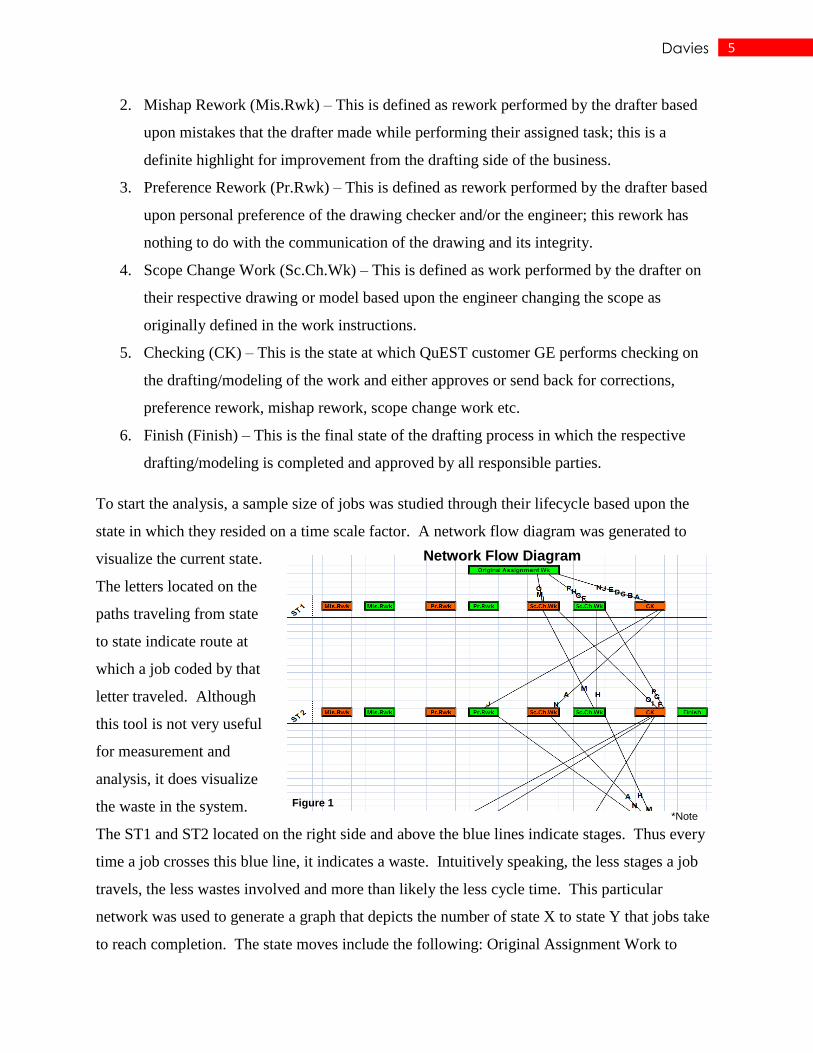
To start the analysis, a sample size of jobs was studied through their lifecycle based upon the

state in which they resided on a time scale factor. A network flow diagram was generated to

visualize the current state.

The letters located on the

paths traveling from state

to state indicate route at

which a job coded by that

letter traveled. Although

this tool is not very useful

for measurement and

analysis, it does visualize

the waste in the system.

The ST1 and ST2 located on the right side and above the blue lines indicate stages. Thus every

time a job crosses this blue line, it indicates a waste. Intuitively speaking, the less stages a job

travels, the less wastes involved and more than likely the less cycle time. This particular

network was used to generate a graph that depicts the number of state X to state Y that jobs take

to reach completion. The state moves include the following: Original Assignment Work to

Network Flow Diagram

Figure 1

*Note

6 Davies

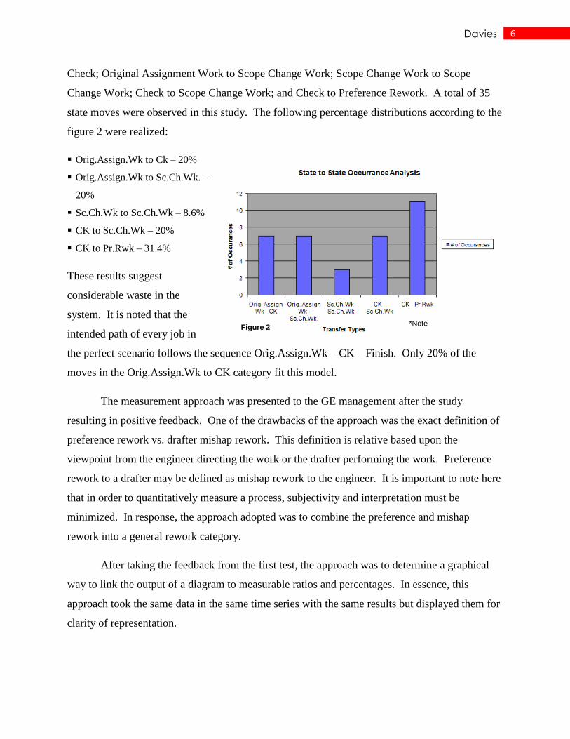
Check; Original Assignment Work to Scope Change Work; Scope Change Work to Scope

Change Work; Check to Scope Change Work; and Check to Preference Rework. A total of 35

state moves were observed in this study. The following percentage distributions according to the

figure 2 were realized:

Orig.Assign.Wk to Ck – 20%

Orig.Assign.Wk to Sc.Ch.Wk. –

20%

Sc.Ch.Wk to Sc.Ch.Wk – 8.6%

CK to Sc.Ch.Wk – 20%

CK to Pr.Rwk – 31.4%

These results suggest

considerable waste in the

system. It is noted that the

intended path of every job in

the perfect scenario follows the sequence Orig.Assign.Wk – CK – Finish. Only 20% of the

moves in the Orig.Assign.Wk to CK category fit this model.

The measurement approach was presented to the GE management after the study

resulting in positive feedback. One of the drawbacks of the approach was the exact definition of

preference rework vs. drafter mishap rework. This definition is relative based upon the

viewpoint from the engineer directing the work or the drafter performing the work. Preference

rework to a drafter may be defined as mishap rework to the engineer. It is important to note here

that in order to quantitatively measure a process, subjectivity and interpretation must be

minimized. In response, the approach adopted was to combine the preference and mishap

rework into a general rework category.

After taking the feedback from the first test, the approach was to determine a graphical

way to link the output of a diagram to measurable ratios and percentages. In essence, this

approach took the same data in the same time series with the same results but displayed them for

clarity of representation.

Figure 2 *Note

7 Davies

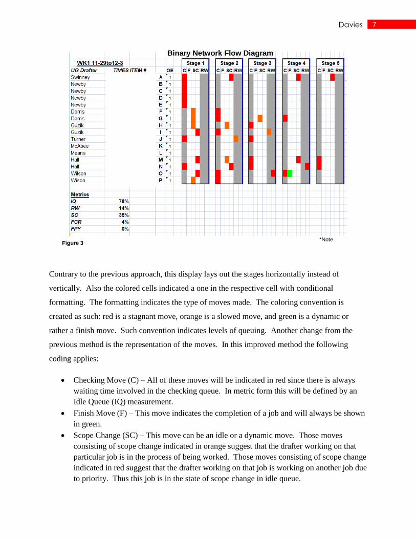
Contrary to the previous approach, this display lays out the stages horizontally instead of

vertically. Also the colored cells indicated a one in the respective cell with conditional

formatting. The formatting indicates the type of moves made. The coloring convention is

created as such: red is a stagnant move, orange is a slowed move, and green is a dynamic or

rather a finish move. Such convention indicates levels of queuing. Another change from the

previous method is the representation of the moves. In this improved method the following

coding applies:

Checking Move (C) – All of these moves will be indicated in red since there is always

waiting time involved in the checking queue. In metric form this will be defined by an

Idle Queue (IQ) measurement.

Finish Move (F) – This move indicates the completion of a job and will always be shown

in green.

Scope Change (SC) – This move can be an idle or a dynamic move. Those moves

consisting of scope change indicated in orange suggest that the drafter working on that

particular job is in the process of being worked. Those moves consisting of scope change

indicated in red suggest that the drafter working on that job is working on another job due

to priority. Thus this job is in the state of scope change in idle queue.

Figure 3

Binary Network Flow Diagram

*Note

8 Davies

Rework Move (RW) – This move can also be an idle or a dynamic move just like scope

change, thus it can be represented in orange or red respectively.

The gray columns under C and RW indicate potential improvement opportunities from the

drafter perspective. Operational soundness can be generally indicated by a minimized number of

moves in these regions. It must be understood that jobs could move in this region from factors

outside control of drafting. Case by case investigation would determine such since preferential

and mishap factors are no longer displayed as in the original approach method.

On the lower left hand corner of Figure 3 above, a metrics table is compiled of critical to

quality (CTQ) metrics for the particular instant in time that the study was performed. A brief

description of each of these metrics is listed as follows below. Note that there are a few metrics

that were explained as moves previously. This explanation involves ratios related to the moves:

Idle Queue Move Ratio (IQ) – This metric relates the number of idle moves made to this

point in time to the total move made. On the graph, all idle moves are indicated in red.

Mathematically it is (idle moves/total moves). In the example above the IQ = 78%.

Rework Move Ratio (RW) – This metric relates the number of rework moves to the total

moves made. Mathematically this metric is derived from the operation (rework

moves/idle moves). In the example above the RW = 14%.

Scope Change Ratio (SC) – This metric is resultant of relating the number of scope

change moves to the total moves. Mathematically this metric is derived from the

operation (scope change moves/total moves). In the example above the SC = 35%.

Finish to Check Ratio (FCR) – This metric is the ratio of the number of finish moves

compared to the number of checking moves. Mathematically this metric is derived from

the operation (finish moves/checking moves). In the example above the FCR = 4%.

First Pass Yield (FPY) – This metric is the ratio of the number of jobs that went to

checking the first time and moved to finish the same time. In the example above the FPY

= 0%.

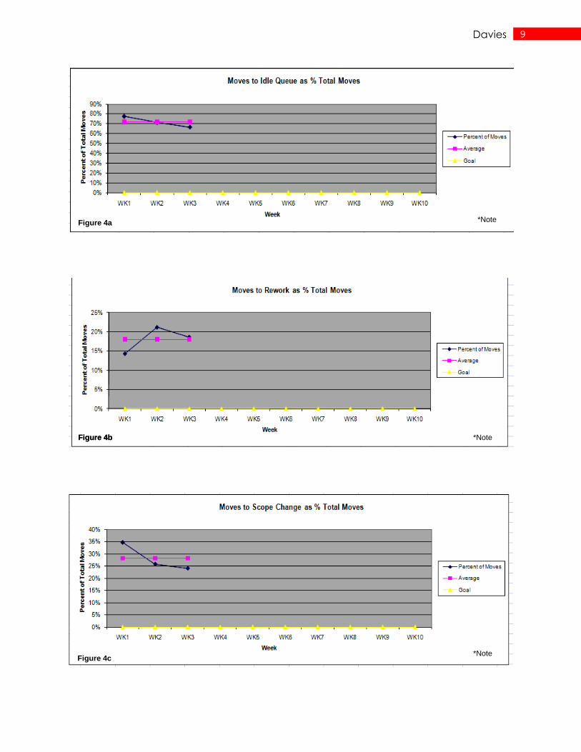
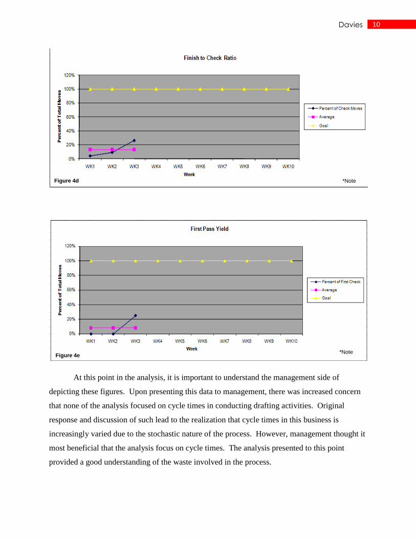
The data results provided in this test suggest serious operational problems. The goal for IQ, RW,

and SC is 0% and that of FCR and FPY is 100%. The study went further to gather these metrics

for a series of three weeks and plotted the progression to validate any trends and capture the

average performance level.

9 Davies

Figure 4c

Figure 4b Figure 4b

Figure 4a

*Note

*Note

*Note

10 Davies

At this point in the analysis, it is important to understand the management side of

depicting these figures. Upon presenting this data to management, there was increased concern

that none of the analysis focused on cycle times in conducting drafting activities. Original

response and discussion of such lead to the realization that cycle times in this business is

increasingly varied due to the stochastic nature of the process. However, management thought it

most beneficial that the analysis focus on cycle times. The analysis presented to this point

provided a good understanding of the waste involved in the process.

Figure 4e

Figure 4d

*Note

*Note

11 Davies

Phase 2

Prior to performing the data analysis, the GE PDE group was using a process log to

record cycle times of activities. Due to the complexity of the tool, not much research was

conducted on the integrity of data that the tool generated. The tool consisted of multiple

automation features compiled on an excel spreadsheet. Usage of the tool appeared to give too

much subjectivity to interpretation due to a lack of constraint on the human aspect of its usage.

However, management insisted that the research would analyze the data generated from this tool

in search of the current state of performance. It must be pointed out that the search for the

optimal solution is a journey and sometime not an easy one. The researcher tried to convince

management that the data generated from this tool would not yield true direction since human

behavior of fudging the data input was not adequately constrained. However, the approach was

to go through the rigger of analyzing the data and let the results speak for itself.

The data from the process logs was compiled manually by selecting a random sample of

388 logs and generating a table of data with times associated with categories such as drafter work

time, scope change time, checking time etc. This data was then analyzed using Minitab as seen

in the below graphs:

Figure 5a

Figure 5a Figure 5b *Note *Note

12 Davies

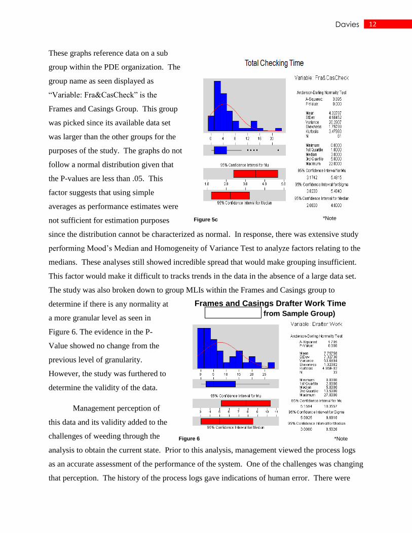
These graphs reference data on a sub

group within the PDE organization. The

group name as seen displayed as

“Variable: Fra&CasCheck” is the

Frames and Casings Group. This group

was picked since its available data set

was larger than the other groups for the

purposes of the study. The graphs do not

follow a normal distribution given that

the P-values are less than .05. This

factor suggests that using simple

averages as performance estimates were

not sufficient for estimation purposes

since the distribution cannot be characterized as normal. In response, there was extensive study

performing Mood’s Median and Homogeneity of Variance Test to analyze factors relating to the

medians. These analyses still showed incredible spread that would make grouping insufficient.

This factor would make it difficult to tracks trends in the data in the absence of a large data set.

The study was also broken down to group MLIs within the Frames and Casings group to

determine if there is any normality at

a more granular level as seen in

Figure 6. The evidence in the P-

Value showed no change from the

previous level of granularity.

However, the study was furthered to

determine the validity of the data.

Management perception of

this data and its validity added to the

challenges of weeding through the

analysis to obtain the current state. Prior to this analysis, management viewed the process logs

as an accurate assessment of the performance of the system. One of the challenges was changing

that perception. The history of the process logs gave indications of human error. There were

Figure 5c

Figure 6

Frames and Casings Drafter Work Time

(0805,0706,0705 from Sample Group)

*Note

*Note

13 Davies

daily reports provided to management of the status of every drafter’s job based on their

respective process logs. In the fields of the process logs, drafters indicated their best estimate of

respective durations. Once a step such as “checking” with an estimated duration was crossed in

time, the real duration was not being captured. In essence, this tool was designed to be a

planning and a data capture tool all at once. Understanding the dynamics of this gave the

researcher the indication that human behavior is to stay out of the spot light, thus there is a

tendency to “fudge” the number to stay off a report. The researcher brought this factor to

management as a potential disclaimer of the data residing in the process logs. Management was

not receptive of this idea as a possible reason for error in the data. The first response of

management was that the real problem was with drafter behavior. The researcher attempted to

steer management away from this perception. While behavior is a factor, it must not be coerced

in process design, it must be constrained. As industrial engineers it is essential to understand

human behavior as it relates to system performance and data representation. The approach taken

from this was to continue the analysis on the process log data and let simple intuition of

relationships be compared to the data.

Some simple regression analysis was performed to determine if intuitive relationships

between variables was realized. The first relationship tested was the drafter work time imputed

in the log versus the applied hours in the database connected to the drafter time record system.

Intuition would suggest that as the drafter work time increases so does the total hours applied.

Figure 7a shows this relationship. The plot shows that there is no relationship between the two

variables under study as evidenced by the R-Sq = 7.8%. This fact suggests that there is potential

Figure 7a Figure 7b *Note *Note

14 Davies

for human error in the data input on the logs and/or likewise on the drafter time record in the

database. Such evidence indicated to the research effort that using the process log data would be

inaccurate for activity duration measurement and planning. However, the research team

continued the analysis to verify the errors in the process log data. Figure 7b portrays the

relationship between time for engineering input to scope change time. Again intuitively, change

in scope is a direct correlation of the time it take for engineering to revise inputs. However, the

data portrayed shows R-Sq = 23.7%. Again, the results portray that the data within the process

logs were insufficient.

Phase 3

Given the results from the process logs, the research had to change direction of which the

search was to determine an accurate estimate of the current state of the system for selected

activities within the PDE organization. At this point in the analysis, research was conducted on

the database that houses all the activities on the schedule and captures the charges in hours to

those respective activities or in GE language manufacturing line item (MLI). Data was extracted

from this database for selected MLIs over a four year period (February 1, 2007 – February 1,

2011). The two variables analyzed in the study were duration in days and actual hours charged.

These two variables would help determine on-time delivery and productivity. Each MLI studied

has a respective drafting item and an engineering item respectively. Drafting items are

designated by numbers while engineering items are designated with their same connected

drafting item with an “E” tagged to the end. It is important to note that the values stream for any

complete drafting job starts with an engineering item and ends with a drafting item. In dumping

this data, both the engineering and drafting item was captured simultaneously. This data was

then sorted accordingly to fit the engineering in front of the drafting item in order to capture the

exact duration of the drafting item. The results as known previously still showed immense

spread in the data as seen in Figure 8 for MLI# 0961. This returns the research to the fact that

the data is so spread that simple averages would do little for measurement purposes – it would

make trend analysis very difficult.

15 Davies

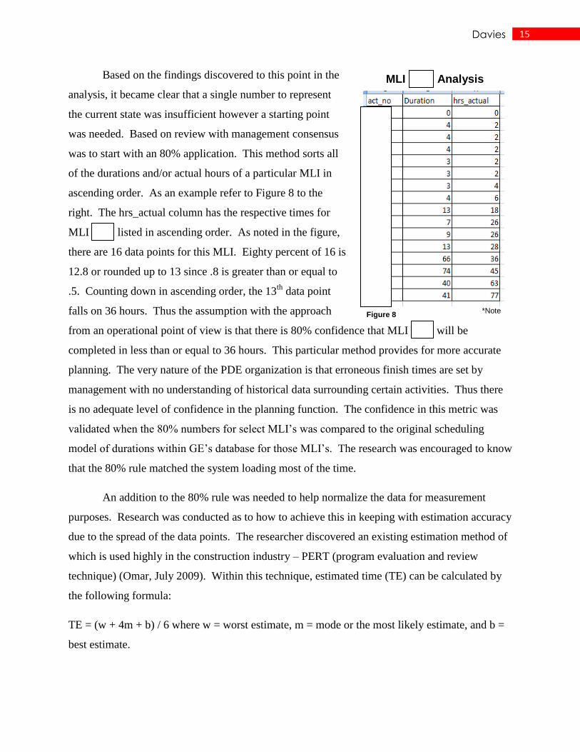
Based on the findings discovered to this point in the

analysis, it became clear that a single number to represent

the current state was insufficient however a starting point

was needed. Based on review with management consensus

was to start with an 80% application. This method sorts all

of the durations and/or actual hours of a particular MLI in

ascending order. As an example refer to Figure 8 to the

right. The hrs_actual column has the respective times for

MLI 0961 listed in ascending order. As noted in the figure,

there are 16 data points for this MLI. Eighty percent of 16 is

12.8 or rounded up to 13 since .8 is greater than or equal to

.5. Counting down in ascending order, the 13th

data point

falls on 36 hours. Thus the assumption with the approach

from an operational point of view is that there is 80% confidence that MLI 0961 will be

completed in less than or equal to 36 hours. This particular method provides for more accurate

planning. The very nature of the PDE organization is that erroneous finish times are set by

management with no understanding of historical data surrounding certain activities. Thus there

is no adequate level of confidence in the planning function. The confidence in this metric was

validated when the 80% numbers for select MLI’s was compared to the original scheduling

model of durations within GE’s database for those MLI’s. The research was encouraged to know

that the 80% rule matched the system loading most of the time.

An addition to the 80% rule was needed to help normalize the data for measurement

purposes. Research was conducted as to how to achieve this in keeping with estimation accuracy

due to the spread of the data points. The researcher discovered an existing estimation method of

which is used highly in the construction industry – PERT (program evaluation and review

technique) (Omar, July 2009). Within this technique, estimated time (TE) can be calculated by

the following formula:

TE = (w + 4m + b) / 6 where w = worst estimate, m = mode or the most likely estimate, and b =

best estimate.

Figure 8

MLI 0961 Analysis

*Note

16 Davies

Note that the application of the worst and best estimate applied was based on the 95%

confidence. In the example of the data given in Figure 8 the WA (weighted average) or TE (time

estimate) of the hrs_actual for MLI 0961 is as follows:

TE = (63+4(2) +0) / 6 TE = 11.8 ~ 12 hour.

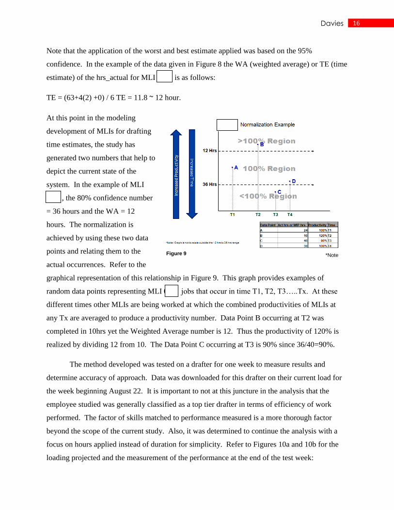
At this point in the modeling

development of MLIs for drafting

time estimates, the study has

generated two numbers that help to

depict the current state of the

system. In the example of MLI

0961, the 80% confidence number

= 36 hours and the WA = 12

hours. The normalization is

achieved by using these two data

points and relating them to the

actual occurrences. Refer to the

graphical representation of this relationship in Figure 9. This graph provides examples of

random data points representing MLI 0961 jobs that occur in time T1, T2, T3…..Tx. At these

different times other MLIs are being worked at which the combined productivities of MLIs at

any Tx are averaged to produce a productivity number. Data Point B occurring at T2 was

completed in 10hrs yet the Weighted Average number is 12. Thus the productivity of 120% is

realized by dividing 12 from 10. The Data Point C occurring at T3 is 90% since 36/40=90%.

The method developed was tested on a drafter for one week to measure results and

determine accuracy of approach. Data was downloaded for this drafter on their current load for

the week beginning August 22. It is important to not at this juncture in the analysis that the

employee studied was generally classified as a top tier drafter in terms of efficiency of work

performed. The factor of skills matched to performance measured is a more thorough factor

beyond the scope of the current study. Also, it was determined to continue the analysis with a

focus on hours applied instead of duration for simplicity. Refer to Figures 10a and 10b for the

loading projected and the measurement of the performance at the end of the test week:

Figure 9 *Note

17 Davies

According the 80% Max metric Employee C is loaded 17.3 hours/day for MLI 0909. This

loading is indicated by orange suggesting a risk in this item closing on its current due date of

August 25. The orange shading also projects the loading out to a suggested revised LFD based

upon loading of 8 hrs/day. This indicates that the date should be moved to September 1. At the

end of the test, this MLI was finally

completed on September 1. Such a

reality provided potential evidence

that the approach was valid. Also at

the end of the test week, the

performance of the WIP and

completed jobs under drafter C was

measured. The results are shown in

Figure 11. Note in this figure that

there are several activities – 1602 and

1623 – that are duplicated. These are

instances in which the same activity is

performed on similar gas turbine

units. In these cases, the approach was to test a heuristic by combining the actual hours of both

Figure 10b

Figure 11

Figure 10a

Employee C Loading Projection

*Note

*Note

*Note

18 Davies

activities into one and increasing the metric for the activity by 20%. This was chosen since a

duplication of activities for similar machines usually involves a “Save As” operation, thus

requiring less time for the second similar activity. It must be understood that this is a random

heuristic test to start as a baseline. Given this assumption the measured productivity for

Employee C for the test week averaged to 91%. At the macro level, this seems fair and

reasonable. However, importance was placed on the items that exceeded the 80% metrics values

such as MLIs 096101 and 1602. This highlights opportunities for improvement. The test and

subsequent results were presented to management for feedback and discussion. Positive reaction

was prevalent however; management proposed that the approach be applied to a team of drafters

within the PDE organization and compare

one team such as CTQ to another sub team.

Such a test required substantial data mining

and analysis along with rigorous excel

functions. However, this test would give

management a better understanding and view

of individual team performance as well as

loading. A test was implemented on the

research group for a week to ascertain the

response of the approach to the perceived loading and performance. This method was also

applied to a second group simultaneously to understand competing group and how they

measured accordingly. The two groups were teams CTQ and GEIQ respectfully. Team CTQ

was the control group and team GEIQ was the comparison group. At the end of the test week the

results were realized according to Figure 12. An important comparison in these graphs is the

earned hours per head. It was agreed that the 80% metric be the earned hours applied to a given

Figure 12

Weekly Comparison of Team’s

Performance

*Note

19 Davies

job once completed. CTQ being the research group possessed earned hours/head = 11.4 while

GEIQ was earned hours/head = 25 respectively. Another indicative measurement was cost

performance index (CPI) where CTQ’s was 44% while GEIQ’s was 92%. These metrics suggest

that the overall performance of GEIQ is better that CTQ. It is important to note that these are the

results of performance of the closed activities for the week under study. Management was very

receptive to this approach as it had been the first time that a more granular measurement has

been applied to stochastically driven processes in the PDE organization. The top manager was

so impressed with the approach that he asked for the research to be expanded and applied his

whole team of over 300 drafters so as to report to senior executive level management.

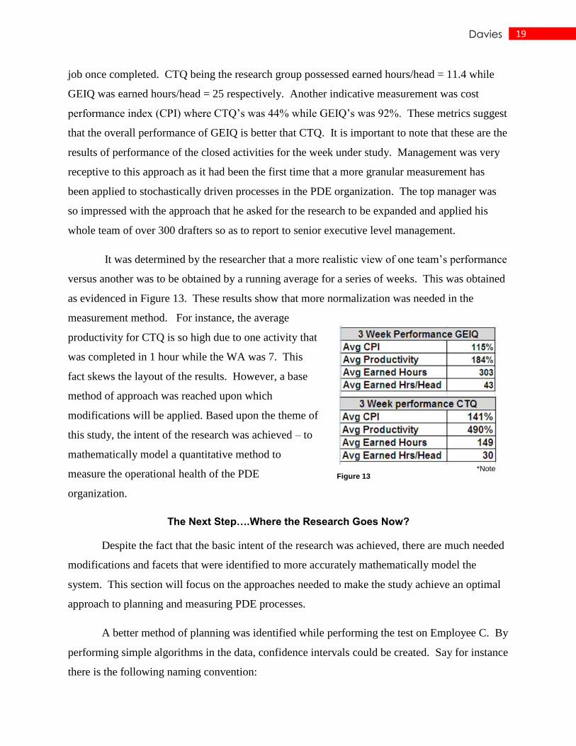
It was determined by the researcher that a more realistic view of one team’s performance

versus another was to be obtained by a running average for a series of weeks. This was obtained

as evidenced in Figure 13. These results show that more normalization was needed in the

measurement method. For instance, the average

productivity for CTQ is so high due to one activity that

was completed in 1 hour while the WA was 7. This

fact skews the layout of the results. However, a base

method of approach was reached upon which

modifications will be applied. Based upon the theme of

this study, the intent of the research was achieved – to

mathematically model a quantitative method to

measure the operational health of the PDE

organization.

The Next Step….Where the Research Goes Now?

Despite the fact that the basic intent of the research was achieved, there are much needed

modifications and facets that were identified to more accurately mathematically model the

system. This section will focus on the approaches needed to make the study achieve an optimal

approach to planning and measuring PDE processes.

A better method of planning was identified while performing the test on Employee C. By

performing simple algorithms in the data, confidence intervals could be created. Say for instance

there is the following naming convention:

Figure 13 *Note

20 Davies

Drafter Name – Drafter X

Job Name – X1,X2…..

Due Date – DX1(for X1), DX2(for X2)……

There is an array of jobs loaded on Drafter X. If this array of X1 and X2 are running in parallel,

there would also be DX1 and DX2 respectfully. If for instance that DX1 is before DX2, then

allow 8 hours per day up to DX1. Then begin from the DX1+1 the same method for X2. Thus if

for example there were 2 days for DX1 and 5 days for DX2, then the hours applied for job X1

would be 16 hours and for job X2 24 hrs respectfully. The 5 is subtracted from the 2 since the

drafter is working on job X1 before job X2. The 16hrs and 24hrs for the respective job’s MLIs

are added to the hours already applied to their respective jobs. This new number of total

estimated hours falls within a percentile range once compared to the array study from the MLIs

once arranged in ascending order. Much like the 80% confidence, this would generate a level of

confidence that the job would be completed by the current due date. Theoretically, this method

would assist in level loading the work load for planning purposes.

Another opportunity was identified for optimal application

of the methods developed in the research. Refer to Figure 14 as

used prior on page 15 of this research. Note in this figure that five

of the data points 2 – 7 took 2hrs to complete. Management

suggested that the history of these data points should be researched

to determine factors that caused this MLI to take 2hrs instead of the

other hours in the array. Furthermore, there could be another layer

of normalization applied to the hours that fall within a heuristic set

number of sigma’s range to determine common denominators

among job groups. If this in-depth research were conducted, the planning function in the study

would generate more granular output of loading among drafters.

Conclusion

The findings from this research have yielded considerable gains in understanding the

drafting process at the GE Gas Turbines Product Definition Engineering Division. The research

Figure 14

MLI 0961 Analysis

*Note

21 Davies

was subdivided into a series of phases representing methodical stages in a heuristic approach to

find the optimal solution. Each phase within the search was the result of an elimination of the

previous phase. The intent of the research was met – to create a mathematical model of the

drafting process that is accepted by management for planning and measurement purposes. Even

though there are improvements to the approach needed, it is understood that there will always be

a search for the “optimal”.

The results of this study are fairly significant. Recall from the first section, that the study

was performed by an employee for QuEST – a contractor for GE. By the end of the third phase

of this research, GE management noted that the method produced from this study was more

accurate than the method used and developed by GE employees. The end intent of this is to

highlight the waste so QuEST can mathematically prove to GE the savings that can be yielded

once improvements are made to the process. As an industrial engineer, the researcher

understands that the value of this work is in the money that can be saved based upon the methods

generated from the analysis. Now that GE has agreed to an approach of measurement, the

researcher feels certain that there is over a 1 million/year that can be saved from using this

method as a planning and measurement tool. The top GE PDE manager, Craig Humanchuk,

made the following statement regarding the results from this study: “It was an analysis that has

never been done in the past and will be a game changer for how GE PDE will run its business in

the future. It will give us a better way to monitor when our process gets off track.”

22 Davies

References and Notes

Omar, Anwar (July 1, 2009) Uncertainty in Project Scheduling – Its Use in PERT/CPM

Conventional Techniques, Cost Engineering Vol. 51/No. 7 July 2009, retrieved from:

http://ehis.ebscohost.com.prox.lib.ncsu.edu/ehost/pdfviewer/pdfviewer?sid=7a85b964-

558c-49be-bf24-7f2dc8593788%40sessionmgr113&vid=2&hid=120

*Note: Data and Graphical representations were generated with approval from related companies

using related company’s software packages such as Minitab, PowerPoint, and Excel for the

completion of this project.