DEVELOPING AN IMAGE RECOGNITION ALGORITHM FOR FACIAL AND DIGIT IDENTIFICATION

Christian Cosgrove, Kelly Li, Rebecca Lin,

Shree Nadkarni, Samanvit Vijapur, Priscilla Wong, Yanjun Yang, Kate Yuan, Daniel Zheng

Advisor: Minjoon Kouh Assistant: Michael Clancy

ABSTRACT

As computers are pushing the limits to reach what seem to be singularly human capabilities, image recognition is at the forefront of scientific efforts. This study aimed to develop an image recognition algorithm that focused on two functionalities: digit recognition and facial recognition. To achieve these objectives, three databases were used in this study: MNIST dataset of handwritten digits, the AT&T image database of grayscale face photos, and a custom database of color photos of 40 New Jersey Governor’s School Scholars (NJGSS). The algorithm extracted quantitative features from these images by calculating average intensity and applying convolutions on the image patches, and it determined the identity of the test images by comparing this information to that of training images. On the MNIST digits database, the image recognition algorithm performed optimally with 588 features, producing an accuracy of 91%. On the AT&T database of grayscale faces, the performance of the algorithm was optimal at 480 features, producing an accuracy of 99% ± 0.67%. On the NJGSS database, the algorithm with 360 features produced an accuracy of 96% ± 1.20%. However, future developments, such as allowing the prioritization of features and the disregard of non­distinguishing features, can still be made to improve the image recognition algorithm. INTRODUCTION

Machine learning employs algorithms that can find patterns from exemplars and make

data­driven predictions. Thus, computers have the ability to learn and act without being given explicit directions by mimicking the human cognitive framework of collecting and applying knowledge to make decisions. In this process, a computer’s performance can improve with experience (1). The concept of machine learning is essential to image recognition algorithms because a computer cannot recognize every possible form of an object, so by having a database of labeled images to train the computer to seek patterns among variations of objects, the computer can “learn” to classify similar objects more effectively. For example, a computer can be taught to recognize the letter “A” by defining the angle of intersection of the three lines that compose the letter, or the ratio of line lengths. Though this representation may be an efficient way to generate the letter, it is not suitable for classification because it does not handle the large amount of variation the letter “A” can have (Fig. 1).

[7­1]

Figure 1 (Sample letter A’s): Examples of variations of the letter “A.”

Machine learning, instead of using an explicit definition, provides a computer with a large number of sample “A’s”, and the computer can classify an input by its similarities and differences to the “A’s” in the pre­existing database. In effect, the computer is being implicitly “taught” the various ways that capital “A” can be written, and can thus recognize the letter through examples.

Neuroscience suggests that humans recognize objects in images first by detecting color, luminance, and texture to separate the objects into their basic shapes, and then by matching the image to a memory (2). While the human mind analyzes images based on large­scale memory and sensory association, computers process objects expressed numerically as vectors and matrices. For instance, computers interpret and display images as matrices of pixel values, with each number representative of the pixel intensity. Despite the different ways in which humans and computers view and process images, some of their methods for recognizing images are the same, specifically edge detection. In humans, the primary visual cortex, located in the occipital cortex of the brain, is responsible for processing visual stimuli. It is associated with edge detection, or locating boundaries where the image intensity changes sharply (3). Neuroscientists David Hubel and Torsten Wiesel noticed that rectangular bars of light more effectively stimulated neurons in the retina than circular spots of light, illustrating the role of edge detection in vision (4). Edge detection algorithms mimic the activity of the visual cortex by searching for discontinuities in intensity to determine changes in material, depth, or orientation. This study hopes to “teach” a computer, through machine learning, to parse inputs in the form of images and identify each image by mirroring the image recognition patterns observed in the human mind.

Image recognition can be broken down into two steps: feature extraction and

classification. Feature extraction quantifies aggregate characteristics of an image, making it easier for a computer program to conduct analysis by obtaining meaningful numbers. Although less information is contained in features than in pixels, features can be specific enough for comparison and generalization. Classification uses the data from feature extraction to sort images into groups. Based on the labels and features of training images, a model can be created to predict the label of a new image.

[7­2]

ALGORITHMS Feature Extraction

Feature extraction is the technique of deriving values, or features, from raw data, so that

an image can be represented numerically. The result of feature extraction is an organized list of numbers, known as a vector. Features such as intensity and gradient are useful for image classification because they are effective at defining characteristics for large­scale patterns in brightness as well as for small areas of contrast, and they are also simple to calculate numerically. There are many different features that can be extracted, and taking a combination, or vector, of multiple features can optimize recognition of images. Extracting too few features prevents the algorithm from distinguishing between classes. However, extracting too many features makes an algorithm too dependent on noise in images, causing it to either overfit the data and to never learn. Therefore, it is important to find the right balance between selectivity, which makes classifications more distinct, and tolerance, which allows for more deviation within a particular class of images.

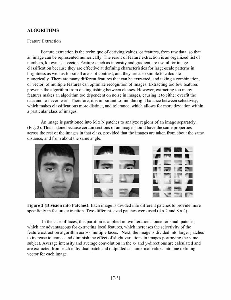
An image is partitioned into M x N patches to analyze regions of an image separately. (Fig. 2). This is done because certain sections of an image should have the same properties across the rest of the images in that class, provided that the images are taken from about the same distance, and from about the same angle.

Figure 2 (Division into Patches): Each image is divided into different patches to provide more specificity in feature extraction. Two different­sized patches were used (4 x 2 and 8 x 4).

In the case of faces, this partition is applied in two iterations: once for small patches, which are advantageous for extracting local features, which increases the selectivity of the feature extraction algorithm across multiple faces. Next, the image is divided into larger patches to increase tolerance and diminish the effect of slight variations in images portraying the same subject. Average intensity and average convolution in the x­ and y­directions are calculated and are extracted from each individual patch and outputted as numerical values into one defining vector for each image.

[7­3]

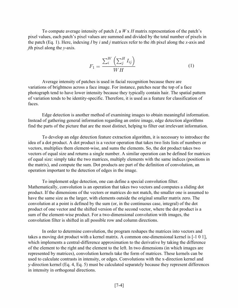
To compute average intensity of patch I, a W x H matrix representation of the patch’s pixel values, each patch’s pixel values are summed and divided by the total number of pixels in the patch (Eq. 1). Here, indexing I by i and j matrices refer to the ith pixel along the x­axis and jth pixel along the y­axis.

Average intensity of patches is used in facial recognition because there are variations of brightness across a face image. For instance, patches near the top of a face photograph tend to have lower intensity because they typically contain hair. The spatial pattern of variation tends to be identity­specific. Therefore, it is used as a feature for classification of faces.

Edge detection is another method of examining images to obtain meaningful information. Instead of gathering general information regarding an entire image, edge detection algorithms find the parts of the picture that are the most distinct, helping to filter out irrelevant information.

To develop an edge detection feature extraction algorithm, it is necessary to introduce the idea of a dot product. A dot product is a vector operation that takes two lists lists of numbers or vectors, multiplies them element­wise, and sums the elements. So, the dot product takes two vectors of equal size and returns a single number. A similar operation can be defined for matrices of equal size: simply take the two matrices, multiply elements with the same indices (positions in the matrix), and compute the sum. Dot products are part of the definition of convolution, an operation important to the detection of edges in the image.

To implement edge detection, one can define a special convolution filter.

Mathematically, convolution is an operation that takes two vectors and computes a sliding dot product. If the dimensions of the vectors or matrices do not match, the smaller one is assumed to have the same size as the larger, with elements outside the original smaller matrix zero. The convolution at a point is defined by the sum (or, in the continuous case, integral) of the dot product of one vector and the shifted version of the second vector, where the dot product is a sum of the element­wise product. For a two­dimensional convolution with images, the convolution filter is shifted in all possible row and column directions.

In order to determine convolution, the program reshapes the matrices into vectors and

takes a moving dot product with a kernel matrix. A common one­dimensional kernel is [­1 0 1], which implements a central­difference approximation to the derivative by taking the difference of the element to the right and the element to the left. In two dimensions (in which images are represented by matrices), convolution kernels take the form of matrices. These kernels can be used to calculate contrasts in intensity, or edges. Convolutions with the x­direction kernel and y­direction kernel (Eq. 4, Eq. 5) must be calculated separately because they represent differences in intensity in orthogonal directions.

[7­4]

Directional changes in the image can be represented in terms of two Prewitt kernels (Eq. 2 ­ 5), where denotes convolution and is a matrix image. Again, the same indexing conventions have been used. These convolutions calculate the intensity gradient of the image. Along an axis, when a strong contrast of light and dark appears (such as those along the eyes, nose, or mouth), the area of change is noted and compared with those of other photos. Before being averaged over a patch, the absolute value of the convolution is taken, preventing changes with opposite signs from canceling out. This leads to more meaningful feature values.

The equations so far explained (containing formulas for F1, F2, F3) are the three

components of an individual patch’s features. Before this information is relayed to the classification algorithm, these features are concatenated into a single­column feature vector. In other words, F4, F5, F6 correspond to patch 2, F7, F8, F9 to patch 3, and so on. The number of dimensions in which the feature vectors reside is therefore three times the number of patches times the number of color components in the image (1 for grayscale, 3 for full color). Classification

Each feature extracted from each patch represents a dimension on a scatterplot. Each photo can then be plotted as a point on this multi­dimensional plot, and if those features are informative enough, the photos containing the same object are likely to form a cluster. A new point can be compared to the existing clusters to find the appropriate match. Figure 3 illustrates this idea in the case of two features.

One of the two classification techniques that this study utilized was the Nearest Neighbor

(NN) method. This technique finds one pre­existing data point that is closest in Euclidean distance to the new, unknown point. For a given pair of feature vectors A and B, the Euclidean distance DED between A and B is defined in terms of the expression (Eq. 6)

[7­5]

where d is the number of feature dimensions. The class to which this nearest point belongs is outputted as the predicted label of the unknown point.

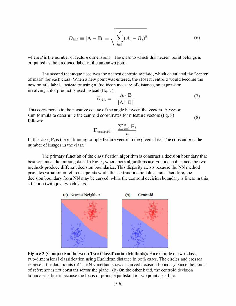
The second technique used was the nearest centroid method, which calculated the “center

of mass” for each class. When a new point was entered, the closest centroid would become the new point’s label. Instead of using a Euclidean measure of distance, an expression involving a dot product is used instead (Eq. 7):

This corresponds to the negative cosine of the angle between the vectors. A vector sum formula to determine the centroid coordinates for n feature vectors (Eq. 8) follows:

In this case, Fi is the ith training sample feature vector in the given class. The constant n is the number of images in the class.

The primary function of the classification algorithm is construct a decision boundary that

best separates the training data. In Fig. 3, where both algorithms use Euclidean distance, the two methods produce different decision boundaries. This disparity exists because the NN method provides variation in reference points while the centroid method does not. Therefore, the decision boundary from NN may be curved, while the centroid decision boundary is linear in this situation (with just two clusters).

Figure 3 (Comparison between Two Classification Methods): An example of two­class, two­dimensional classification using Euclidean distance in both cases. The circles and crosses represent the data points (a) The NN method shows a curved decision boundary, since the point of reference is not constant across the plane. (b) On the other hand, the centroid decision boundary is linear because the locus of points equidistant to two points is a line.

[7­6]

Confusion Matrix

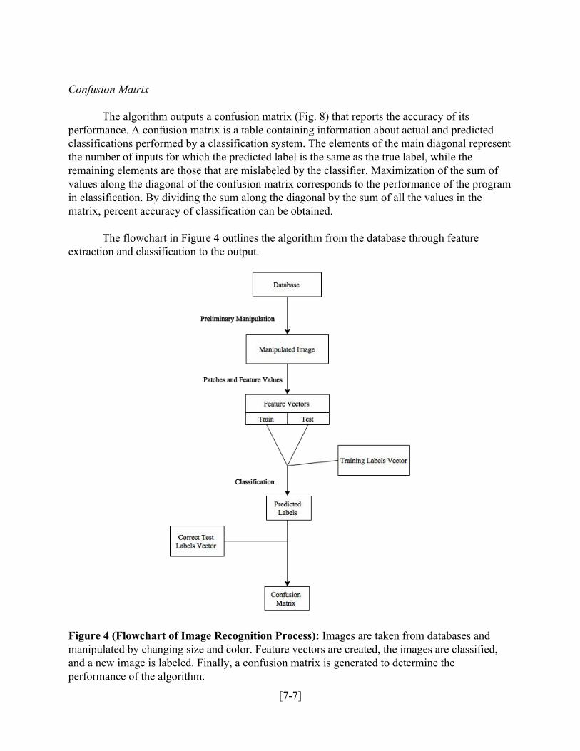
The algorithm outputs a confusion matrix (Fig. 8) that reports the accuracy of its performance. A confusion matrix is a table containing information about actual and predicted classifications performed by a classification system. The elements of the main diagonal represent the number of inputs for which the predicted label is the same as the true label, while the remaining elements are those that are mislabeled by the classifier. Maximization of the sum of values along the diagonal of the confusion matrix corresponds to the performance of the program in classification. By dividing the sum along the diagonal by the sum of all the values in the matrix, percent accuracy of classification can be obtained.

The flowchart in Figure 4 outlines the algorithm from the database through feature extraction and classification to the output.

Figure 4 (Flowchart of Image Recognition Process): Images are taken from databases and manipulated by changing size and color. Feature vectors are created, the images are classified, and a new image is labeled. Finally, a confusion matrix is generated to determine the performance of the algorithm.

[7­7]

IMPLEMENTATION OF ALGORITHMS Digit Recognition Databases

The database used for digit analysis was a subset of the MNIST (Mixed National Institute of Standards and Technology) Database, consisting of 515 28 x 28 grayscale images of digits 0 to 9 (Fig. 5, Ref. 5). Out of this initial database, 430 images were separated from the rest to form a training set, and the remaining 85 were compiled into a test set. The images within this database looked similar to the digits that they depicted, but varied enough from one another for the program to examine many different writing styles and to allow for effective generalization.

Figure 5 (MNIST Database Digits): Examples of 28 x 28 digit images from the MNIST Database.

Facial Recognition Database

A portion of the face photos were compiled from the AT&T Laboratories Cambridge grayscale faces database (“The Database of Faces”), with 40 subjects and 10 photos for each subject. The images were taken in varying positions against a dark, homogeneous background. The size of each image is 112 x 92 pixels, and each pixel has an intensity value between 0 and 255 (6, 7). The NJGSS Database was created to match the format of the AT&T database, with 40 subjects of 10 photos each, and with each photo taken against a dark backdrop and resized to be 112 x 92 pixels (Fig. 6). In addition, each image was taken at a slightly different angle to train the computer to recognize various orientations of faces.

[7­8]

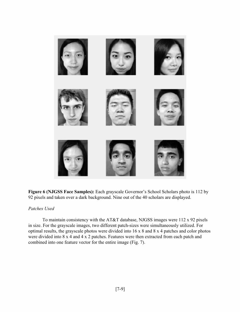
Figure 6 (NJGSS Face Samples): Each grayscale Governor’s School Scholars photo is 112 by 92 pixels and taken over a dark background. Nine out of the 40 scholars are displayed. Patches Used

To maintain consistency with the AT&T database, NJGSS images were 112 x 92 pixels

in size. For the grayscale images, two different patch­sizes were simultaneously utilized. For optimal results, the grayscale photos were divided into 16 x 8 and 8 x 4 patches and color photos were divided into 8 x 4 and 4 x 2 patches. Features were then extracted from each patch and combined into one feature vector for the entire image (Fig. 7).

[7­9]

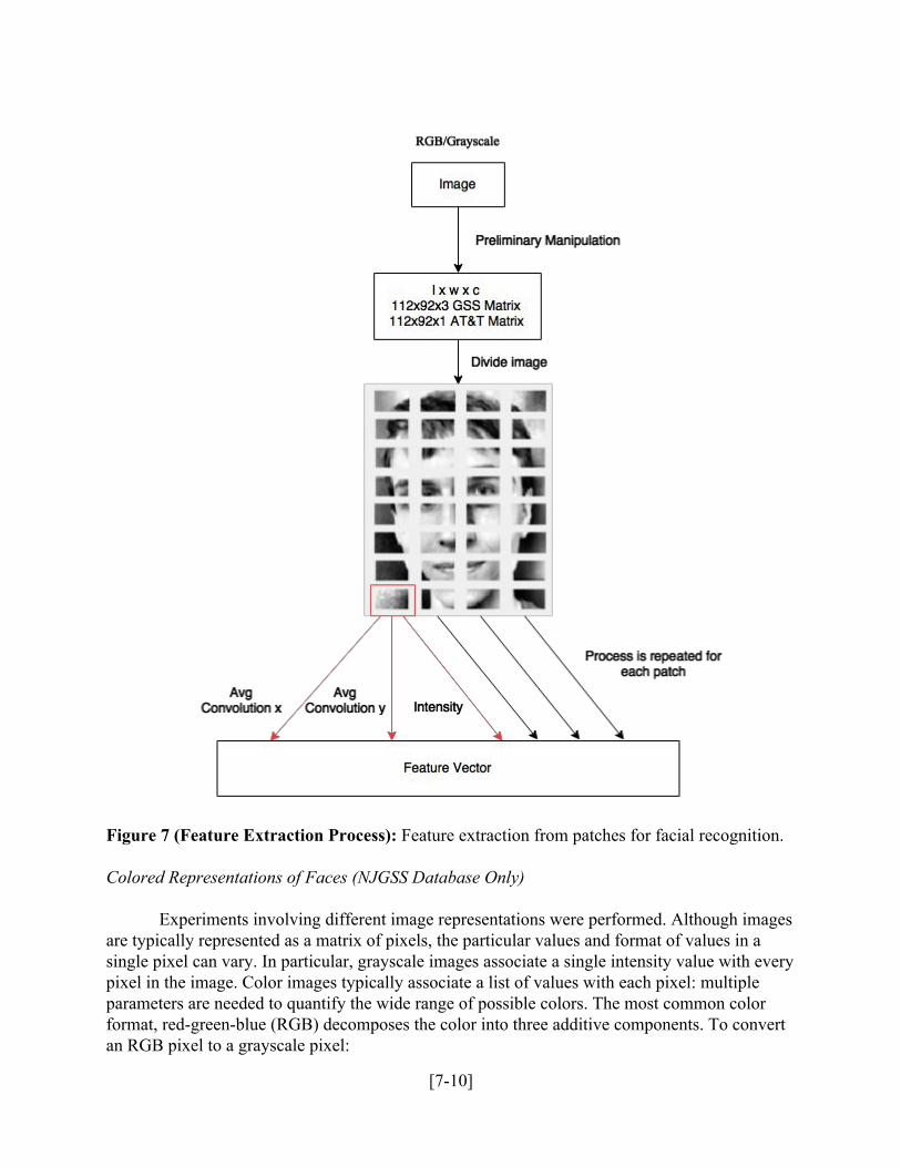
Figure 7 (Feature Extraction Process): Feature extraction from patches for facial recognition. Colored Representations of Faces (NJGSS Database Only)

Experiments involving different image representations were performed. Although images are typically represented as a matrix of pixels, the particular values and format of values in a single pixel can vary. In particular, grayscale images associate a single intensity value with every pixel in the image. Color images typically associate a list of values with each pixel: multiple parameters are needed to quantify the wide range of possible colors. The most common color format, red­green­blue (RGB) decomposes the color into three additive components. To convert an RGB pixel to a grayscale pixel:

[7­10]

Y represents the grayscale intensity, which is expressed as a function of the

individual RGB channel intensities. Since this function is not invertible, information is lost when combining the channels into one value.

As an alternative to RGB, HSV is another way of parameterizing pixel colors. In HSV,

hue is a quantity that approximately represents which color the pixel contains, while saturation and value are quantities typically associated with lighting conditions.

RESULTS

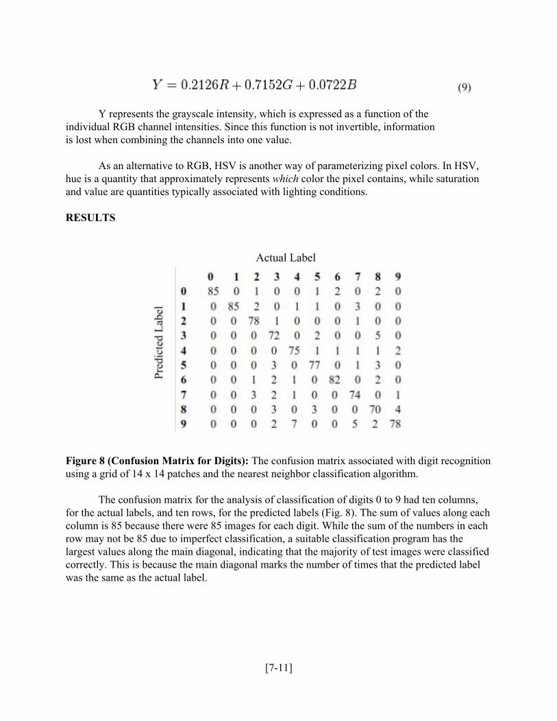
Figure 8 (Confusion Matrix for Digits): The confusion matrix associated with digit recognition using a grid of 14 x 14 patches and the nearest neighbor classification algorithm.

The confusion matrix for the analysis of classification of digits 0 to 9 had ten columns,

for the actual labels, and ten rows, for the predicted labels (Fig. 8). The sum of values along each column is 85 because there were 85 images for each digit. While the sum of the numbers in each row may not be 85 due to imperfect classification, a suitable classification program has the largest values along the main diagonal, indicating that the majority of test images were classified correctly. This is because the main diagonal marks the number of times that the predicted label was the same as the actual label.

[7­11]

To determine the optimal number of patches and the relationship between number of

patches and performance, images were divided into varying numbers of patches. As mentioned earlier, different sizes of patches allow the algorithm to follow features of various scales. As a function of number of patches, digit classification accuracy tended to increase with both algorithms (Fig. 9). With only one patch, NN classification yielded only 40% accuracy while centroid classification yielded 30%. As the number of patches increased, so did the accuracy of classification. However, both algorithms did not exceed a certain accuracy threshold: the NN classifier did not exceed 92% accuracy, and the centroid classifier did not exceed 78%. While nearest neighbors always outperformed centroid classification for a given number of patches, it scaled differently with the number of patches; after a 14 x 14 patch grid was used, the accuracy of the nearest­neighbor algorithm decreased. This is not observed with the centroid algorithm: from Figure 9, centroid classification appears to approach 78% monotonically.

Figure 9 (Graph of Digit Classification Accuracy): Displays percent accuracy for nearest­neighbor and centroid classification of digit images using N x N patches, 430 training images and 85 test images.

Similar quantitative tests were performed on the face database. In Fig. 10, one can see the percent accuracy of the NN algorithm for face recognition. Like digit classification, accuracy tends to increase with the number of patches. However, in face classification, centroids both increases and decreases after it reaches a maximum instead of becoming asymptotically constant.

[7­12]

Figure 10 (Graph of AT&T Classification Accuracy): Displays percent accuracy for nearest­neighbor and centroid classification of grayscale faces from the AT&T database.

Figure 11 (Graph of Facial Identification Accuracy): Displays percent accuracy of the facial classification program using varying amounts of training pictures for HSV, RGB, and grayscale images.

[7­13]

For facial recognition, another variable was color format. Three color formats were tested: grayscale, RGB, and HSV. To see how these representations compare to each other as well as how they scale with size of dataset, the accuracies of these representations were assessed as a function of number of training samples. Figure 11 shows the accuracy of the algorithm versus number of training samples.

According to this graph, the RGB and HSV formats were nearly equivalent in performance. However, grayscale representation tended to perform 20% worse than color representations on average. Another notable feature of the grayscale representation is that it continues to increase in accuracy after the color algorithms have already plateaued.

Performance for facial recognition was measured in a similar fashion to that of digit recognition by utilizing a confusion matrix. However, by interpreting the confusion matrix as an graph­theoretic adjacency matrix, a more meaningful graphical representation of the faces could be obtained. The adjacency matrix establishes the strength of similarities between displayed the faces of test subjects on a network. Thicker connectors indicate more similarities detected between faces (Fig. 12).

Figure 12 (Web of Facial Recognition Accuracy): A graph of Governor’s School Scholars showing similarities between scholars. Thicker lines represent higher similarity.

[7­14]

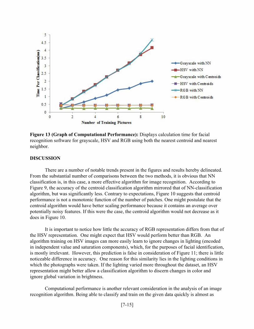
Figure 13 (Graph of Computational Performance): Displays calculation time for facial recognition software for grayscale, HSV and RGB using both the nearest centroid and nearest neighbor. DISCUSSION

There are a number of notable trends present in the figures and results hereby delineated. From the substantial number of comparisons between the two methods, it is obvious that NN classification is, in this case, a more effective algorithm for image recognition. According to Figure 9, the accuracy of the centroid classification algorithm mirrored that of NN­classification algorithm, but was significantly less. Contrary to expectations, Figure 10 suggests that centroid performance is not a monotonic function of the number of patches. One might postulate that the centroid algorithm would have better scaling performance because it contains an average over potentially noisy features. If this were the case, the centroid algorithm would not decrease as it does in Figure 10.

It is important to notice how little the accuracy of RGB representation differs from that of

the HSV representation. One might expect that HSV would perform better than RGB. An algorithm training on HSV images can more easily learn to ignore changes in lighting (encoded in independent value and saturation components), which, for the purposes of facial identification, is mostly irrelevant. However, this prediction is false in consideration of Figure 11; there is little noticeable difference in accuracy. One reason for this similarity lies in the lighting conditions in which the photographs were taken. If the lighting varied more throughout the dataset, an HSV representation might better allow a classification algorithm to discern changes in color and ignore global variation in brightness.

Computational performance is another relevant consideration in the analysis of an image

recognition algorithm. Being able to classify and train on the given data quickly is almost as

[7­15]

important as the accuracy of the algorithm. Accuracy sometimes must be sacrificed for performance time, or practicality. Although MATLAB is not the most efficient programming language and the implementation is not optimized for performance, it is still possible to extract meaningful information about the computational complexity of the algorithm by measuring the execution time of classification. In Figure 13, NN took significantly longer to classify individual images than the centroid method. Linear complexity is expected because distance computations must be performed between the test image and all of the training samples to find the nearest neighbor. Conversely, only a constant number of distance calculations must be performed in centroid classification, so constant complexity is expected. Therefore, for a given amount of computation time, centroid classification provides more accuracy. Furthermore, whereas for the centroid algorithm it remained roughly constant, execution time increased linearly with number of training samples.

Another trend seen in the picture is that using RGB and HSV channels separately

significantly increases performance of the classification algorithm compared to using grayscale. (Fig. 11). The loss of color data in conversion from RGB to grayscale causes a decrease in the accuracy of classification. Conversions between RGB and HSV conserve information and are invertible, and thus results in similar accuracies. The run time of the classification algorithm on grayscale images is significantly less than the run time on RGB and HSV images. This is due to the reduced amount of information present in a grayscale image, which results in fewer features extracted and fewer comparisons. CONCLUSIONS

In summary, this image recognition algorithm consists of two general steps: feature extraction and classification. To generate a set of meaningful, independent quantities, the images were divided into a set of patches, with all the relevant features extracted from each patch. With these defining qualities, the computer could recognize different classes (labels for either digits or faces). The accuracy of the algorithm increased monotonically with the number of training samples. Of the classification techniques employed, the NN method proved more effective than centroid, although the centroid method was significantly faster. Nearest neighbor classification reached a maximum earlier than centroid due to the NN’s following of subtle changes in training data. Based on these results, it is clear that a future algorithm should use NN if accuracy is paramount (unless there is a situation with extreme amounts of overlapping training points). If, on the other hand, an algorithm is to have faster performance, centroid classification is favorable.

Other improvements can be made to the algorithm in the future in both feature extraction

and classification. Classification can be optimized by using a k­Nearest­Neighbors algorithm, a generalization of the current Nearest Neighbors algorithm, which takes into account multiple nearest neighbors (the traditional NN method is where k=1). The k­Nearest­Neighbors algorithm increases the tolerance of the classification algorithm because it diminishes the effect of outliers in the training set by requiring more reference points. Additionally, as the algorithm was developed, it became clear that some elements in feature vectors were less important than others (certain features, when run independently, proved more accurate than others). In fact, some features did not contribute at all to improve accuracy. To make room for more expressive

[7­16]

features, an improved algorithm would include a procedure to prune redundant or non­distinguishing features from vectors.

Personal security measures, such as those for electronic devices or home

protection­involving image recognition, are becoming increasingly common, but this same field also has wide applications in the sciences. As systems become increasingly sophisticated, image recognition algorithms could identify tumors or chromosomal abnormalities. Matching current images of a patient to those accumulated in a database comprised of previous cases, diagnoses would be speed up dramatically. By recognizing issues earlier and more accurately, this technology could dramatically increase chances of survival. REFERENCES

1. Sajda P. Machine learning for detection and diagnosis of disease. Annu. Rev. Biomed. Eng. 2006;8:537­565.

2. Biederman I. Recognition­by­components: a theory of human image understanding. Psychol. Rev. 1986;94(2):115­147.

3. Marr D, Hildreth E. Theory of edge detection. Royal Soc. Publ. 1980;207(1167):187­217. 4. Hubel DH, Wiesel TN. Receptive fields, binocular interaction and functional architecture

in the cat’s visual cortex. J. Physiol. 1962;160(1):106­154. 5. MNIST Database of Handwritten Digits [Internet]. [cited 2015 Jul 29]. Available from:

http://yann.lecun.com/exdb/mnist/ 6. The Database of Faces [Internet]. 2002. AT&T Laboratories Cambridge; [cited 2015 Jul

29]. Available from: http://www.cl.cam.ac.uk/research/dtg/attarchive/facedatabase.html 7. Samaria FS, Harter AC. Parameterisation of a stochastic model for human face

identification. Appl. Comput. Vis. 1994:138­142.

[7­17]