digital simulation of dynamic systemsdynamic...
TRANSCRIPT

Karadeniz Technical UniversityDepartment of Electrical and Electronics Engineering
61080 Trabzon, Turkey
Chapter 6-1
, y
Digital Simulation of Dynamic SystemsDynamic Systems
Bu ders notları sadece bu dersi alan öğrencilerin kullanımına açık olup,üçüncü sahıslara verilmesi, herhangi bir yöntemle çoğaltılıp başka
İyerlerde kullanılması, yayınlanması Prof. Dr. İsmail H. ALTAŞ’ın yazılıiznine tabidir. Aksi durumlarda yasal işlem yapılacaktır.
Chapter 6-2

Chapter 6-3
Digital SimulationDigital Simulation
Diff. Equation Laplace Transform Digital Simulation
May be used for the first and secont order systems. The process will be complicated for higher order systems
The easiest way to obtain the time response of a system.
Time Domain Response
Chapter 6-4
Euler integration
Simpson’s Rule
Trapezoid Rule of Integration
Differences: • Running speed• Accuracy• Programming difficulties• etc...
Euler Digital integrationEuler Digital integration
11 −− += nnn rTyyTrapezoid Rule of integrationTrapezoid Rule of integration
( )11 2 −− ++= nnnn rrT
yy
Simpson Rule of IntegrationSimpson Rule of Integration
( )212 4 3 −−− +++= nnnnn rrrT
yy
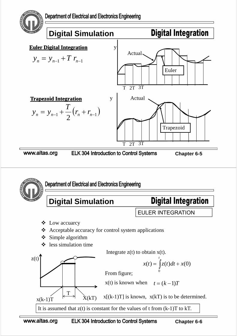
y : outputr : inputT : sampling period
Digital Simulation
Chapter 6-5
T 2T 3T
Actual
Euler
y
T 2T 3T
Actual
Trapezoid
y
Euler Digital IntegrationEuler Digital Integration
11 −− += nnn rTyy
Trapezoid IntegrationTrapezoid Integration
( )11 2 −− ++= nnnn rrT
yy
Digital Simulation
Chapter 6-6
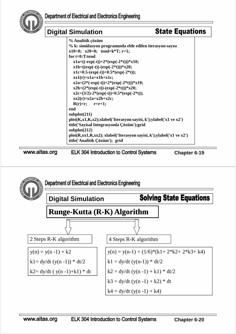
Low accuarcyAcceptable accuracy for control system applicationsSimple algorithmless simulation time
Integrate z(t) to obtain x(t).
∫ +=t
xdttztx0
)0()()(
From figure;
Tkt )1( −=x(t) is known when
x[(k-1)T] is known, x(kT) is to be determined.
It is assumed that z(t) is constant for the values of t from (k-1)T to kT.
Tx(k-1)T X(kT)
z(t)
Digital SimulationEULER INTEGRATION

Chapter 6-7
])1[(])1[()( TkTzTkxkTx −+−=
∫ +=t
xdttztx0
)0()()(
T(k-1)T kT
z(t)
A
B
In this equation, x(kT), is an approximate of x(t) with the steps t=kT. As shown in figure, only the area represented by A is considered and the area represented by B is ignored. Therefore this method is also called Rectangular integration.
In simulation the differential equations are integrated. In the above equations z(t) is the derivative of x(t).
Digital SimulationEULER INTEGRATION
Chapter 6-8
0)()( =+ txtx&
Use Euler integration to obtain a solution for the above equation. Assume the initial condition x(0)=1 and sampling period as 0.1.
The analytical solution of this diff. Equation is: x(t)=e-t
0)()( =+ txtx& )()()( txtxtz −== &
{ }])1[(])1[()( TkxTTkxkTx −−+−=
Sampling period, T=0.1
Digital Simulation
EULER INTEGRATION

Chapter 6-9
{ }])1[(])1[()( TkxTTkxkTx −−+−=
( )( )( )
( ) 3487.0)9.0(9.0)0.1(
..................
729.0)81.0)(1.0(81.0)2.0(2.0)3.0(
81.0)9.0)(1.0(9.0)1.0(1.0)2.0(
9.0)0.1)(1.0(1)0(0)1.0(
=−=
=−=−==−=−=
=−=−=
Txxx
Txxx
Txxx
Txxx
For T=0.1 and k=1 .........10 the solution is
Since the analytical solution is known, we can check the accuracy of the results for t=1 sec.
3678.0)1()( 1 ==== −− eextx t
What would happen if we use T=0.01 sec. instead of T=0.1.
Search the effect of T on the simulation time and the accuracy of the result.
Digital Simulation
EULER INTEGRATION
Chapter 6-10
)()()( tButAxtx +=&)0( )()( 1
0
11 xdttxtxt
+= ∫ &
)1( )1()( 111 −+−= kxTkxkx & kT k(k-1)T (k-1)
PS:PS:
AbreviatedThe same equation can be written for any xi(t)element of the state vector
)1()1()( −+−= kxTkxkx iii & ni <<1
This equation can be expressed as a vector.
)1( )1()( −+−= kxTkxkx &
)1()1()1( −+−=− kBukAxkx&where
Digital Simulation

Chapter 6-11
DATA: A, B, T, x(0), k=1
)1()1()1( −+−=− kBukAxkx&
)1( )1()( −+−= kxTkxkx &
K=k+1 ε≤−− )1()( kxkxNO
STOP
Digital Simulation
Chapter 6-12
Obtain a digital solution for the following state equations using Euler Integration
⎥⎦
⎤⎢⎣
⎡+⎥
⎦
⎤⎢⎣
⎡−−
=1
0
02
13xx& [ ]xy 01=
The actual solution is:The actual solution is:
( ) ( )
( ) ( ) tttttt
tttttt
eexeexeetx
eexeexeetx
22
21
22
22
21
21
2
12
2
3)0(2)0(22)(
2
1
2
1)0()0(2)(
−−−−−−
−−−−−−
+−+−++−=
+−+−++−=
Digital simulation
Digital Simulation

Chapter 6-13
Data:Data:⎥⎦
⎤⎢⎣
⎡−−
=02
13A ⎥
⎦
⎤⎢⎣
⎡=
1
0B 0)0()0( 21 == xx
Initial Conditions:
Sampling period: T=0.01 sec. and u(t)=1, Tolerance=0.001
Step 1
⎥⎦
⎤⎢⎣
⎡=⎥
⎦
⎤⎢⎣
⎡+⎥
⎦
⎤⎢⎣
⎡⎥⎦
⎤⎢⎣
⎡−−
=+==−1
01
1
0
0
0
02
13)0()0()0()1( BuAxxkx &&
1=k
⎥⎦
⎤⎢⎣
⎡=⎥
⎦
⎤⎢⎣
⎡+=+=
01.0
0
1
001.00)0()0()1( xTxx &
⎥⎦
⎤⎢⎣
⎡≥⎥
⎦
⎤⎢⎣
⎡=⎥
⎦
⎤⎢⎣
⎡−⎥
⎦
⎤⎢⎣
⎡=−=
001.0
001.0
01.0
0
0
0
01.0
0)0()1( xxε
Digital Simulation
Chapter 6-14
Step 2
⎥⎦
⎤⎢⎣
⎡=⎥
⎦
⎤⎢⎣
⎡+⎥
⎦
⎤⎢⎣
⎡⎥⎦
⎤⎢⎣
⎡−−
=+==−1
01.01
1
0
01.0
0
02
13)1()1()1()1( BuAxxkx &&
21=+= kk
⎥⎦
⎤⎢⎣
⎡=⎥
⎦
⎤⎢⎣
⎡+⎥
⎦
⎤⎢⎣
⎡=+=
02.0
0001.0
1
01.001.0
01.0
0)1()1()2( xTxx &
⎥⎦
⎤⎢⎣
⎡≥⎥
⎦
⎤⎢⎣
⎡=⎥
⎦
⎤⎢⎣
⎡−⎥
⎦
⎤⎢⎣
⎡=−=
001.0
001.0
01.0
0001.0
01.0
0
02.0
0001.0)1()2( xxε
Digital Simulation

Chapter 6-15
⎥⎦
⎤⎢⎣
⎡=⎥
⎦
⎤⎢⎣
⎡+⎥
⎦
⎤⎢⎣
⎡⎥⎦
⎤⎢⎣
⎡−−
=+==−9998.0
0197.01
1
0
02.0
0001.0
02
13)2()2()2()1( BuAxxkx &&
31=+= kk
⎥⎦
⎤⎢⎣
⎡=⎥
⎦
⎤⎢⎣
⎡+⎥
⎦
⎤⎢⎣
⎡=+=
03.0
0003.0
9998.0
0197.001.0
02.0
0001.0)2()2()3( xTxx &
⎥⎦
⎤⎢⎣
⎡≥⎥
⎦
⎤⎢⎣
⎡=⎥
⎦
⎤⎢⎣
⎡−⎥
⎦
⎤⎢⎣
⎡=−=
001.0
001.0
01.0
0002.0
02.0
0001.0
03.0
0003.0)2()3( xxε
Step 3
Digital Simulation
Chapter 6-16
The iteration is stopped when the difference between two consecutive results is smaller than a prescribed tolerance value. The iteration process must be done in a computer.
k x1 x2k x1 x21.0000 0 0.01002.0000 0.0001 0.02003.0000 0.0003 0.03004.0000 0.0006 0.04005.0000 0.0010 0.05006.0000 0.0014 0.06007.0000 0.0020 0.06998.0000 0.0026 0.07999.0000 0.0034 0.0898
10.0000 0.0042 0.0998
The first 10 iteration
Digital Simulation

Chapter 6-17
Digital Simulation
%*************************************************% SYSTEM SIMULATION - euler_01.m%*************************************************clear% VERILER
A=[ -3 1; -2 0]; B=[0; 1]; C=[ 1 0]; D=0; u=1; T=0.1; % Initial Values
x10=0; x20=0; E=1000; k=1; % Iterationwhile E > 0.00001
dx1=A(1,1)*x10+A(1,2)*x20+B(1)*u;dx2=A(2,1)*x10+A(2,2)*x20+B(2)*u;x1(k)=x10+T*dx1; x2(k)=x20+T*dx2;E1=abs(x1(k)-x10); E2=abs(x2(k)-x20);E=max(E1,E2);x10=x1(k); x20=x2(k); K(k)=k;
k=k+1;endplot(K,x1,K,x2,’o’); xlabel('Iteration Counter, k'); ylabel('x1 and x2');grid
Chapter 6-18
Digital Simulation
Chapter 6-19
% Analitik çözüm% k: simülasyon programında elde edilen iterasyon sayısıx10=0; x20=0; tend=k*T; r=1;for t=0:T:tend
x1a=((-exp(-t))+2*(exp(-2*t)))*x10;x1b=((exp(-t))-(exp(-2*t)))*x20;x1c=0.5-(exp(-t))+0.5*(exp(-2*t));xx1(r)=x1a+x1b+x1c;x2a=(2*(-exp(-t))+2*(exp(-2*t)))*x10;x2b=(2*(exp(-t))-(exp(-2*t)))*x20;x2c=(3/2)-2*(exp(-t))+0.5*(exp(-2*t));xx2(r)=x2a+x2b+x2c;R(r)=r; r=r+1;
endsubplot(211)plot(K,x1,K,x2);xlabel('Iterasyon sayisi, k');ylabel('x1 ve x2')title('Sayisal Integrasyonla Çözüm');gridsubplot(212)plot(R,xx1,R,xx2); xlabel('Iterasyon sayisi, k');ylabel('x1 ve x2')title('Analitik Çözüm'); grid
Digital Simulation
Chapter 6-20
RungeRunge--Kutta (RKutta (R--K) AlgorithmK) Algorithm
2 Steps R-K algorithm 4 Steps R-K algorithm
y(n) = y(n -1) + k2
k1= dy/dt (y(n -1)) * dt/2
k2= dy/dt ( y(n -1)+k1) * dt
y(n) = y(n-1) + (1/6)*(k1+ 2*k2+ 2*k3+ k4)
k1 = dy/dt (y(n-1)) * dt/2
k2 = dy/dt (y(n -1) + k1) * dt/2
k3 = dy/dt (y(n -1) + k2) * dt
k4 = dy/dt (y(n -1) + k4)
Digital Simulation

Chapter 6-21
4 Step R4 Step R--K algorithmK algorithm
6
)(2
),(*
)2
,2
(*
)2
,2
(*
),(*
43211
34
23
12
1
kkkkxx
kxTtfTk
kx
TtfTk
kx
TtfTk
xtfTk
nn
nn
nn
nn
nn
++++=
++=
++=
++=
=
+
T: Sampling period
n : Iteration counter
t : time
xn : Variable to be found
f : the function that uses the variable x and the time.
Digital Simulation
Chapter 6-22
Use Runge-Kutta algorithm to solve the following state equations. Note that these equations were solved before using Euler’s integration.
⎥⎦
⎤⎢⎣
⎡+⎥
⎦
⎤⎢⎣
⎡−−
=1
0
02
13xx&
[ ]xy 01=
Sampling period: dt=T=0.01 sec., Input : u(t)=1,
Tolerance=0.001
Digital Simulation

Chapter 6-23
%***************************************% inputsA=[ -3 1
-2 0 ];B=[0; 1]; C=[ 1 0]; D=0;% initials for simulationx10=0; x20=0;u1=0; u2=1;dt=0.01; tend=5;t0=0; k=1; % k is iteration counter.%****************************************
Section 1: Data and Initial Conditions
Digital Simulation
Chapter 6-24
while t0<tend-dtx11=x10; x21=x20;a1=dt*( A(1,1)*x11 + A(1,2)*x21 + B(1,1)*u1);a2=dt*( A(2,1)*x11 + A(2,2)*x21 + B(2,1)*u2);x12=x10+a1/2; x22=x20+a2/2;b1=dt*( A(1,1)*x11 + A(1,2)*x21 + B(1,1)*u1);b2=dt*( A(2,1)*x11 + A(2,2)*x21 + B(2,1)*u2);x13=x10+b1/2; x23=x20+b2/2;c1=dt*( A(1,1)*x11 + A(1,2)*x21 + B(1,1)*u1);c2=dt*( A(2,1)*x11 + A(2,2)*x21 + B(2,1)*u2);x14=x10+c1; x24=x20+c2;d1=dt*( A(1,1)*x11 + A(1,2)*x21 + B(1,1)*u1);d2=dt*( A(2,1)*x11 + A(2,2)*x21 + B(2,1)*u2);
x1(k)=x10+(a1+2*b1+2*c1+d1)/6;x2(k)=x20+(a2+2*b2+2*c2+d2)/6;
U(k)=u1; t(k)=t0+dt; t0=t(k);x10=x1(k); x20=x2(k); k=k+1;
end;
Section 2: Runge Kutta algorithm
Digital Simulation

Chapter 6-25
subplot(211)plot(t,x1);title('x1');xlabel('time in seconds'):ylabel('x1');gridsubplot(212)plot(t,x2);title('x2');xlabel('time in seconds'):ylabel('x2');grid
Section 3: Plot the results
Digital Simulation
Chapter 6-26
0 0.5 1 1.5 2 2.5 3 3.5 4 4.5 50
0.1
0.2
0.3
0.4
0.5
time in seconds
x1
0 0.5 1 1.5 2 2.5 3 3.5 4 4.5 50
0.5
1
1.5
time in seconds
x2
Resultant plots
Digital Simulation

Chapter 6-27
Solve the following state-space equations using 4 step Runge-Kutta algorithm.
Assume input u1(t)=100, u2(t)=0, dt=T=0.01, All initial conditions are zero. Simulate the system for 1 sec. Starting t=0 sec.
1 1 1
2 2 2
4 3 1 0
1 8 0 1
x x u
x x u
− −⎡ ⎤ ⎡ ⎤ ⎡ ⎤⎡ ⎤ ⎡ ⎤= +⎢ ⎥ ⎢ ⎥ ⎢ ⎥⎢ ⎥ ⎢ ⎥−⎣ ⎦ ⎣ ⎦⎣ ⎦ ⎣ ⎦ ⎣ ⎦
&
&
Digital Simulation
[ ] 1
2
( ) 1 0x
y tx
⎡ ⎤= ⎢ ⎥
⎣ ⎦
Chapter 6-28
Digital Simulation
Clear% -------- input data --------------------------------------------------A=[ -4 -3; 1 -8]; B=[1 0; 0 1]; C=[ 0 1]; D=0;u1=100.0; u2=0; dt=0.01; tend=1; t0=0; k=1; % -------- Initial conditions -----------------------------------------U=[u1;u2]; SIZEA=size(A); NL=SIZEA(1); NC=SIZEA(2);for n=1:NL
x0(n)=0;endy0=0;% -------------- start iterative solution
Section 1 – Input data

Chapter 6-29
Digital Simulation
while t0<tend-dt[x]=runge(A,B,U,x0,dt);u(k)=U(1); y(k)=x(1); x1(k)=x(1); x2(k)=x(2); t(k)=t0+dt; t0=t(k);for n=1:NL
x0(n)=x(n); XX(k,n)=x(n); endk=k+1;
end;% -------------------------- Plots
Section 2 – Iteration
Chapter 6-30
Digital Simulation
% -------------------------- Plotssubplot(211)plot(t,u); xlabel('Time (sec.)'); ylabel('u');gridsubplot(212)plot(t,y,t,x1,t,x2 ); xlabel('Time (sec.)'); ylabel('y, x1, x2'); grid
Section 3 – Plots
Chapter 6-31
Digital Simulation
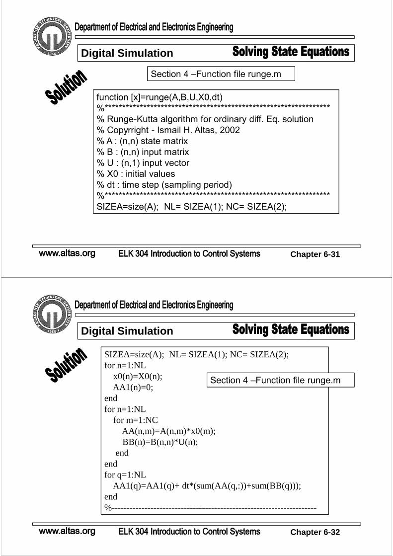
Section 4 –Function file runge.m
function [x]=runge(A,B,U,X0,dt)%****************************************************************% Runge-Kutta algorithm for ordinary diff. Eq. solution% Copyrright - Ismail H. Altas, 2002% A : (n,n) state matrix% B : (n,n) input matrix% U : (n,1) input vector% X0 : initial values% dt : time step (sampling period)%****************************************************************SIZEA=size(A); NL= SIZEA(1); NC= SIZEA(2);
Chapter 6-32
Digital Simulation
SIZEA=size(A); NL= SIZEA(1); NC= SIZEA(2);for n=1:NL
x0(n)=X0(n);AA1(n)=0;
endfor n=1:NL
for m=1:NCAA(n,m)=A(n,m)*x0(m);BB(n)=B(n,n)*U(n);
endendfor q=1:NL
AA1(q)=AA1(q)+ dt*(sum(AA(q,:))+sum(BB(q)));end%--------------------------------------------------------------------
Section 4 –Function file runge.m

Chapter 6-33
Digital Simulation
%--------------------------------------------------------------------for n=1:NL
x0(n)=X0(n)+AA1(n)/2;BB1(n)=0;
endfor n=1:NL
for m=1:NCAA(n,m)=A(n,m)*x0(m);BB(n)=B(n,n)*U(n);
endendfor q=1:NL
BB1(q)=BB1(q)+ dt*(sum(AA(q,:))+sum(BB(q)));end%--------------------------------------------------------------------
Section 4 –Function file runge.m
Chapter 6-34
%--------------------------------------------------------------------for n=1:NL
x0(n)=X0(n)+BB1(n)/2;CC1(n)=0;
endfor n=1:NL
for m=1:NCAA(n,m)=A(n,m)*x0(m);BB(n)=B(n,n)*U(n);
endendfor q=1:NL
CC1(q)=CC1(q)+ dt*(sum(AA(q,:))+sum(BB(q)));end%--------------------------------------------------------------------
Digital Simulation
Section 4 –Function file runge.m

Chapter 6-35
Digital Simulation
%--------------------------------------------------------------------for n=1:NL
x0(n)=X0(n)+CC1(n);DD1(n)=0;
endfor n=1:NL
for m=1:NCAA(n,m)=A(n,m)*x0(m);BB(n)=B(n,n)*U(n);
endendfor q=1:NL
DD1(q)=DD1(q)+ dt*(sum(AA(q,:))+sum(BB(q)));end%--------------------------------------------------------------------
Section 4 –Function file runge.m
Chapter 6-36
Digital Simulation
Section 4 –Function file runge.m
%--------------------------------------------------------------------------for n=1:NL
x(n)=X0(n)+(AA1(n)+2*BB1(n)+2*CC1(n)+DD1(n))/6;end%--------------------------------------------------------------------------

Chapter 6-37
Section 5 –Results
Digital Simulation
Chapter 6-38