does money matter - the national bureau of economic … · · 2001-05-01discontinuities and...

$% !!

!"#&'()

"*++,,,-.#- +""#/+,&'()

0$

1232//4/#/5##

6.7 #82'19&

! "# $% ! & #'!

&! ( "" ) * +

* ," &+- ./! &+//

0- ""1" ' ! - #

$-1"012"

' )3 $0

4 # 00! 2 21""

512"" " 4 0

#/### #///4/6#/:6744#

#:6//4/#/

$ !"#-&'()

'221

#""#/7#/"4;/#;#5#;#74:4##<;=/4#6#874/7#/

,<#//-/8,:4:/##747//"#/4;/7/#4787#/

4#/#7 #74; :7 : /4;; ;,/"#7 7/4/ ;#7 6"5#7 /7#

4#5#6#

/6#/./#75/"#7 4/#7./#7:6;// #/32>3

4#/:#47;;:#747,##/"#/4;/-/6#/;// #/4#/#7

/"#7 6"5#7? 7##//4#/8./,#::#4& 7##//4#/-#

;///,/ 4#/#/ ? 7#5# # #/ /4#/,##//4#7, 6"5#7

"#:64#.;,/4 /7#/-

5#/:4 $

1121/3&##

4 80(2(9>

7$

@- A /.-44 -#7

3

I. INTRODUCTION

Economists and policymakers often cite improving public schools as an effective way to increase

productivity, speed economic growth, and provide economic opportunity to children of the poor.1 The

question of how to improve public schools nonetheless remains open.2 Whether more resources improve

student outcomes remains controversial largely because the observed association between spending and

pupil achievement is generated partly by variation in district characteristics other than spending. Since

public schools in the United States are traditionally controlled and funded at the local level, taste for

education, property tax rates, and labor costs drive much of the variation in education spending. These

variables in turn are related to measures of achievement and attainment.

One source of variation in education spending levels that may help to isolate a causal link

between spending and student outcomes is state equalization schemes. These state laws attempt to

redistribute education funding by giving more state aid to districts that historically spend less on schools.

Since 1971, nearly 40 states have passed such laws. In a recent paper, Murray, Evans and Schwab [1998]

conclude that court-ordered equalization schemes decreased within-state spending inequality by 19 to 34

percent. Card and Payne [1997] also show evidence that the equalization of funding induced by these

laws may have weakened the relationship between test scores and family background.

1 See, for example, Krugman [1994], Schultz [1961, 1980], Duflo [1999], Psacharopoulos [1984], Clinton

[2000].

2 See, for example, Hanushek [1996], Hedges, Laine and Greenwald [1994], Betts [1995], Card and

Krueger [1996].

4

This paper analyzes the effect of educational expenditures on student achievement in the context

of a major equalization law in Massachusetts. This reform redistributed funds across districts using

information on past spending levels, student characteristics, property values, and per-capita income. By

focusing on the experiences of individual districts in one state, this is the first study to exploit exogenous

variation in district-level per-pupil spending to evaluate the effect of expenditures on student

achievement.

The analysis that follows used idiosyncratic variation in state education aid caused by

discontinuities and non-linearities in the state aid formulas of the Massachusetts Education Reform Act of

1993 (MERA) to identify two parameters. First, the idiosyncratic variation in spending is shown to cause

increases in per-pupil spending at the local level. The amount of state education aid passed through to

local per-pupil expenditures is consistent with that predicted by a simple income effect. Second, the

analysis examines whether the additional spending resulting from idiosyncratic increases in state aid

causes improvements in student test scores. The findings suggest that increased funding leads to

improvement in 4th-grade test scores, but show no evidence of an effect on 8th-grade test scores.

In its simplest form, the identification strategy compares school districts on either side of a

discontinuity in the state education aid formula. Districts arbitrarily close to the discontinuity are

assumed to be comparable. The only difference between these districts is that those on one side receive

state aid for education while those on the other side do not. Empirically, a figure shows a sharp drop in

per-pupil spending exactly at this discontinuity of the aid formula.

Though the graphical analysis is appealing, the variance in per-pupil spending and test scores

unexplained by changes in state aid makes drawing statistical inferences difficult. A complementary

identification strategy is to use the aid formula from MERA as an instrument for the increase in per-pupil

spending in the district since 1993. For the aid formula to be a viable instrument two conditions must

hold. First, the aid determined by the formula must be uncorrelated with unobservable determinants of

test scores. And second, conditional on regression controls, the aid determined by the formula must be

correlated with the increase in per-pupil spending.

5

The aid formula may appear a poor candidate for an instrument because it depends on

determinants of student achievement. MERA sets aid as a discontinuous function of observable district

characteristics. However, Campbell and Stanley [1963] suggest that exactly this sort of discontinuous

selection criteria can solve the problem of identifying causal effects. If the outcome of interest does not

directly depend on the covariates in the selection formula discontinuously, then the discontinuity in the

relationship between the outcome and covariates may be attributed to the selection mechanism.

Angrist and Lavy [1999] show that in some cases the regression-discontinuity estimates described

by Campbell and Stanley [1963] correspond to those from a two-stage least squares (2SLS) procedure. In

their case, class-size is a discontinuous function of enrollment. Because test scores are determined in part

by enrollment, a regression of test scores on the class-size function suffers from omitted variables bias.

However, test scores do not directly depend on enrollment in the same discontinuous way the class-size

function does. Thus, the class-size function must have explanatory power for test scores, conditional on a

smooth function of enrollment. Angrist and Lavy [1999] use the class-size function as an instrument for

class size, conditional on a smooth function of enrollment.

Following Campbell and Stanley [1963] and Angrist and Lavy [1999], I show that the

discontinuous aid formula is uncorrelated with unobserved determinants of student achievement,

conditional on smooth functions of the arguments in the aid formula. Thus, the first condition is met.

The second condition concerns how much of each dollar of state education aid is ultimately spent

on schools. However, the correlation of state aid and per-pupil spending, made explicit by equalization

schemes, complicates the estimation of the effective redistribution of school spending. One identification

strategy is to compare changes in per-pupil spending to changes in state education aid. This differencing

strategy, however, does not correct for the correlation of state aid with unobserved time-varying district

characteristics. I show below that if the dispersion in per-pupil spending is increasing over time, it is

likely that the change in state aid is positively correlated with the change in unobserved determinants of

education spending.

6

Again, the aid formula provides a potential solution to this identification problem. The

discontinuity in the aid formula allows it to act as an instrument for the increase in state aid in the

estimation of the effect of state aid on local education spending. Regression-discontinuity estimates show

that increased state aid does lead to increased per-pupil spending. Thus, the second condition is met. In

the end, the graphical analysis and the Two-Stage Least Squares estimation produce remarkably similar

estimates. The estimates suggest that 60 to 75 cents of each dollar of state aid are spent on local

education.

Since the two conditions outlined above are met, the aid formula can be used as an instrument for

the increase in per-pupil spending. Regression-discontinuity estimates suggest that money does matter.

In particular, estimates for 4th-graders are mostly significantly different from zero, and are fairly

consistent across specifications and test subjects. These estimates imply that a one standard deviation

increase in per-pupil spending leads to about a half of a standard deviation increase in 4th-grade test

scores. Further investigation of the effect of per-pupil spending on different points in the test-score

distribution suggests that the increased mean test scores observed among 4th-graders comes as a result of

improvements by low-scoring students. Results for 8th-graders show no evidence of an effect of spending

on mean test scores. Effects on 8th-grade test scores may be smaller because 8th-graders spent a smaller

portion of their education in well-funded schools. This explanation assumes that education is a

cumulative process. Further analysis suggests that increased spending decreases the fraction of 8th-

graders scoring at both tails of the distribution of test scores. Results for both grades therefore support the

notion that the MERA reduced inequality of student achievement.

The paper is organized as follows. The next section presents a description of the Massachusetts

Education Reform Act of 1993. After Section III describes the identification strategy more specifically,

Section IV provides a graphical analysis of the regression-discontinuity identification strategy. Section V

describes the data. Section VI presents estimates of the effect of an additional dollar of state aid for

education on local educational spending. Section VII presents estimates of the effect of an increase in

per-pupil spending on the increase in test scores. Section VIII concludes.

7

II. THE MASSACHUSETTS EDUCATION REFORM ACT

Local property tax based funding exposes public schools to significant variation in resources

across school districts. Passed in 1993, MERA acts to equalize funding for public schools across districts

within the state. MERA distributes aid disproportionately to poorer districts, but does not explicitly tax

current educational expenditures.

MERA bases funding on two concepts: the Foundation Budget and the Gross Standard of Effort.

The Foundation Budget is an estimate of how much the district should spend to provide an adequate

education to its students. The Foundation Budget formula is a function of the number and characteristics

of the students in the district. For instance, the state assumes the cost of educating a special education

student is three times the cost of educating a regular education student.

The Gross Standard of Effort is an estimate of how much the district is able to spend on schools.

The state Department of Revenue calculated the Gross Standard of Effort in 1994 as the amount of tax

revenue that the district would raise with a school property tax rate of 9.4 percent. Each year the state

increases the Gross Standard of Effort by a district-specific growth factor that measures the districts

potential growth in local revenue. Local revenue growth is limited in Massachusetts by Proposition 2 ½,

an initiative passed in 1980 that restricts property tax revenue to be no more than 2 ½ percent of the

districts total property value and restricts property tax revenue growth to 2 ½ percent per annum.

Proposition 2 ½ allows increases above the 2 ½ percent limit for new construction. Districts may also

vote to override the Proposition 2 ½ constraint for the current year. The override increases the base used

for the 2 ½ percent limit calculation.

MERA allocates a fraction of the difference between the Foundation Budget and the Gross

Standard of Effort as supplemental aid. This is called Foundation Aid. The average Foundation award

rose from $408,464 in 1994 to $821,669 in 1998. About one-third of districts receive some Foundation

Aid.

8

Many districts spend significantly less than the Gross Standard of Effort. It is infeasible for these

districts to increase school spending to the Gross Standard of Effort immediately. MERA specifies a

reasonable annual increase in local spending and allocates to these districts a percentage of the gap

between local spending and the Gross Standard of Effort (the Gross Standard of Effort Gap). To direct

state funds to the districts most in need of help, MERA specifies a formula for the percentage of the Gross

Standard of Effort Gap the state allocates as Overburden Aid.

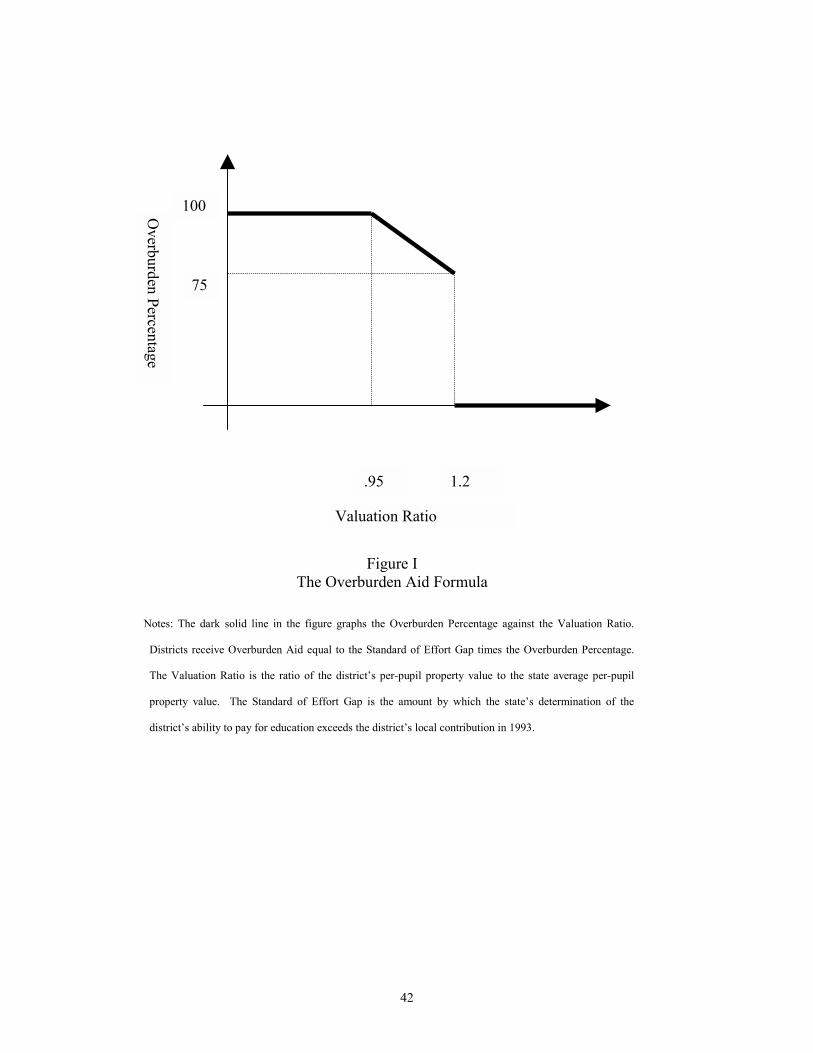
The key determinant of Overburden Aid is the Overburden Percentage. The Overburden

Percentage is a function of the districts Valuation Ratio and the 1989 per-capita income in the district.

MERA defines the Valuation Ratio as the ratio of the districts property value per pupil to the statewide

average of this measure. As illustrated in Figure I, those districts that have a Valuation Ratio less than .95

(i.e. those that have low property values) receive Overburden Aid equal to 100% of the gap between local

spending and the Gross Standard of Effort (the Standard of Effort Gap). Those that have a Valuation

Ratio between .95 and 1.2 get a percentage that declines linearly from 100% to 75%. Districts with

Valuation Ratios above 1.2 receive no Overburden Aid. In fiscal year 1994, those districts with per-

capita income, as measured by the 1990 census, below the statewide average of $17,224 received 100%

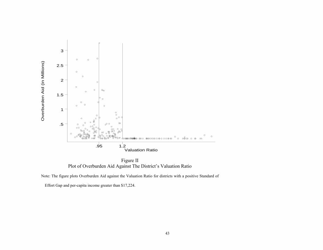
of the Standard of Effort Gap. Figure II shows a plot of Overburden Aid against the Valuation Ratio for

districts with a positive Standard of Effort Gap. The figure shows the sharp cutoff in positive values of

Overburden Aid at the point where the Valuation Ratio is 1.2. Nearly all districts with Valuation Ratios

above 1.2 receive no Overburden Aid.

The total transfer of Overburden Aid has risen from $26.9 million in 1994, the first year after the

passage of the law, to $104.2 million in 1998. The average award rose from $196,857 in 1994 to

$643,383 in 1998. About 30 percent of districts receive some Overburden Aid. Among districts that

received Overburden Aid in 1996, the average district got $179 per pupil. Overburden Aid is

significantly smaller in magnitude than Foundation Aid.

9

III. IDENTIFICATION

The objective of this paper is to use the structure of MERA to identify the effect of education

spending on student achievement. Consider the comparison of an increase in student test scores and an

increase in local education spending. The causal relationship of interest can be written

( ) 00100 sstsstsst EETT ηηγγ −+−+=− (1)

where stT denotes the average test score by students in school district s in fiscal year t, stE denotes per-

pupil spending, and stη is a district-specific error term that varies over time. The increase in school

expenditures may be positively or negatively correlated with 0sst ηη − . For instance, districts with a

large taste for education spending may also invest in the human capital of their children outside of

schools. Alternatively, equalization schemes, which drive some of the variation in 0sst EE − , tax

districts taste for education, which may be included in stη . Thus, Ordinary Least Squares (OLS)

generally yields inconsistent estimates of 1γ .

One solution to the identification problem is to use aid formulas from MERA as instruments for

the increase in education spending. For these formulas to be viable instruments two conditions must be

met. First, conditional on regression controls, the aid formulas must be correlated with the increase in

school spending. Second, conditional on observable district characteristics, the aid formulas must not be

correlated with determinants of student achievement other than education expenditures.

The first condition demands that district-level increases in state aid prescribed by MERA lead to

increases in per-pupil expenditures. Consider the naïve comparison of local education spending per pupil

and state education aid per pupil. The relationship can be written

10

stsstst SE εµββ +++= 10 (2)

where stE denotes per-pupil spending in school district s in fiscal year t, stS denotes per-pupil state aid

for schools transferred to school district s in fiscal year t, sµ represents time-invariant determinants of

per-pupil spending, including the taste for education in the school district, and stε is an error term.

Equalization schemes set stS so that ( ) 0, <sstSCov µ . Thus the OLS estimate of 1β is too low.

One solution is to subtract 0sE from (2) to get

0010 )( sstsstsst SSEE εεβ −+−=− . (3)

The change in state aid, (Sst Ss0), may still be correlated with shifting preferences for education, which

are contained in εst εs0. Controls for economic characteristics, such as the per-capita income, Is0, and a

measure of the districts property tax base, Vst, can be added to (3). Let ρI ( . ) and ρV ( . ) represent any

continuously differentiable function of Is0 and Vst, respectively. The equation to be estimated is now

00010~~)()()( sststVsIsstsst VISSEE εερρβ −+++−=− (4)

where stε~ represents the estimated residual from an OLS regression of stε on )( 0sI Iρ and )( stV Vρ .

However, even conditional on ρI (Is0) and ρV (Vst), the change in state aid per pupil may be correlated with

εst εs0. For instance, if the dispersion in Est is growing over time, ( ) 0,0 >− ssstCov µεε . Since MERA

is more progressive than the aid scheme it replaced, ( ) 0,0 <− ssst SSCov µ . These two facts imply that

Sst Ss0 is negatively correlated with εst εs0, and that the OLS estimate of (4) yields estimates of β1 that

are too low.

11

The formulas used to determine Overburden Aid and Foundation Aid can be used to solve this

endogeneity problem. Denote the formula used to compute Overburden Aid ( ).Ω , and denote the

formula used to compute Foundation Aid ( ).Φ . The relationship of the increase in state aid since the

passage of MERA to the level of Overburden and Foundation Aid can be written

0020100 )()()(),( sstststVsIststssst nVInVISS ννδρρααα −++++Φ+Ω+=− (5)

where nst is the Foundation Enrollment in school district s in fiscal year t, as computed by the state

Department of Education. The discontinuity of ( ).Ω ensures that 01 ≠α . Conditional on nst, ( ).Φ

should have a positive effect on Sst because bilingual and special education students are weighted more in

the foundation budget formula. The state assumes that the cost of educating a special education student is

about three times the cost of educating a regular education student;3 the state assumes the cost of

educating a bilingual education student is about 20 percent more than the cost of educating a regular

education student. If, as Cullen [1997] shows, unfunded requirements to fund special education students

crowd out funding of regular education students, then by funding the education of special needs students

Foundation Aid should lead to increased spending on regular education students. In other words, 2α

should be positive.

If in fact 1α and 2α are nonzero, (5) can be used as a first stage in a two-stage least squares

(2SLS) estimation of (4), because conditional on )( 0sI Iρ , )( stV Vρ and nst, neither ( ).Ω nor ( ).Φ is

correlated with εst εs0. In other words, Overburden Aid can be used as an instrument for the increase in

state aid if the only reason the change in per-pupil spending has the same discontinuous characteristic as

3 This estimate is in line with the estimates in Chaikind (1993), which are reported in Cullen (1997).

12

the change in state aid is because of the discontinuous structure of ( ).Ω .4 Foundation Aid can be used

as an instrument for the increase in state aid if districts with a high number of special education students

have different levels of per-pupil spending, but not different changes in per-pupil spending over time,

apart from the effect of MERA. Empirical estimates of β1 are indeed positive. Thus, the first condition is

met.

The second condition concerns whether ( ).Ω and ( ).Φ are correlated with 0sst ηη − ,

conditional on )( 0sI Iρ , )( stV Vρ and nst. The argument is the same as described above. So long as

0sst TT − does not have the same discontinuous form as ( ).Ω and trends in test scores are unrelated to

enrollments of special education students, the aid formulas are uncorrelated with determinants of student

achievement other than education spending. Thus, the second condition is met, and the MERA aid

formulas can be used as instruments for the increase in per-pupil spending to estimate 1γ . The next

section provides a graphical version of the identification strategy.

IV. GRAPHICAL ANALYSIS

In its most basic form, the identification strategy compares school districts on either side of the

discontinuity created by the Overburden Aid formula. Districts that are close enough to the discontinuity

point are assumed to be comparable. The only difference between these two sets of districts is the

difference in Overburden Aid provided. A simple analysis of what fraction of state education aid is spent

on schools is to see if districts with Valuation Ratios just more than 1.2 spend decidedly less per pupil

than those with ratios just above the cutoff. Remember that districts with Valuation Ratios just above the

cutoff at 1.2 receive no Overburden Aid, while those just below may receive some positive amount.

4 The use of such a regression-discontinuity estimation strategy is derived from Campell and Stanley

(1963), and is described more recently by van Der Klauww (1996) and Angrist and Lavy (1999).

13

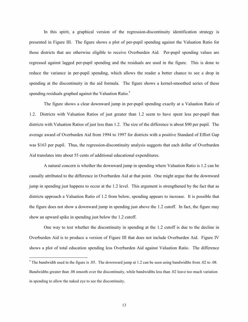
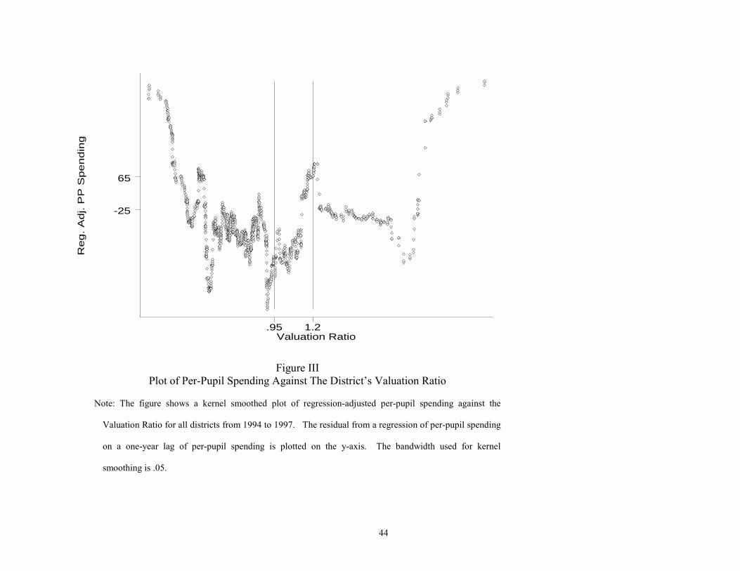
In this spirit, a graphical version of the regression-discontinuity identification strategy is

presented in Figure III. The figure shows a plot of per-pupil spending against the Valuation Ratio for

those districts that are otherwise eligible to receive Overburden Aid. Per-pupil spending values are

regressed against lagged per-pupil spending and the residuals are used in the figure. This is done to

reduce the variance in per-pupil spending, which allows the reader a better chance to see a drop in

spending at the discontinuity in the aid formula. The figure shows a kernel-smoothed series of these

spending residuals graphed against the Valuation Ratio.5

The figure shows a clear downward jump in per-pupil spending exactly at a Valuation Ratio of

1.2. Districts with Valuation Ratios of just greater than 1.2 seem to have spent less per-pupil than

districts with Valuation Ratios of just less than 1.2. The size of the difference is about $90 per pupil. The

average award of Overburden Aid from 1994 to 1997 for districts with a positive Standard of Effort Gap

was $163 per pupil. Thus, the regression-discontinuity analysis suggests that each dollar of Overburden

Aid translates into about 55 cents of additional educational expenditures.

A natural concern is whether the downward jump in spending where Valuation Ratio is 1.2 can be

causally attributed to the difference in Overburden Aid at that point. One might argue that the downward

jump in spending just happens to occur at the 1.2 level. This argument is strengthened by the fact that as

districts approach a Valuation Ratio of 1.2 from below, spending appears to increase. It is possible that

the figure does not show a downward jump in spending just above the 1.2 cutoff. In fact, the figure may

show an upward spike in spending just below the 1.2 cutoff.

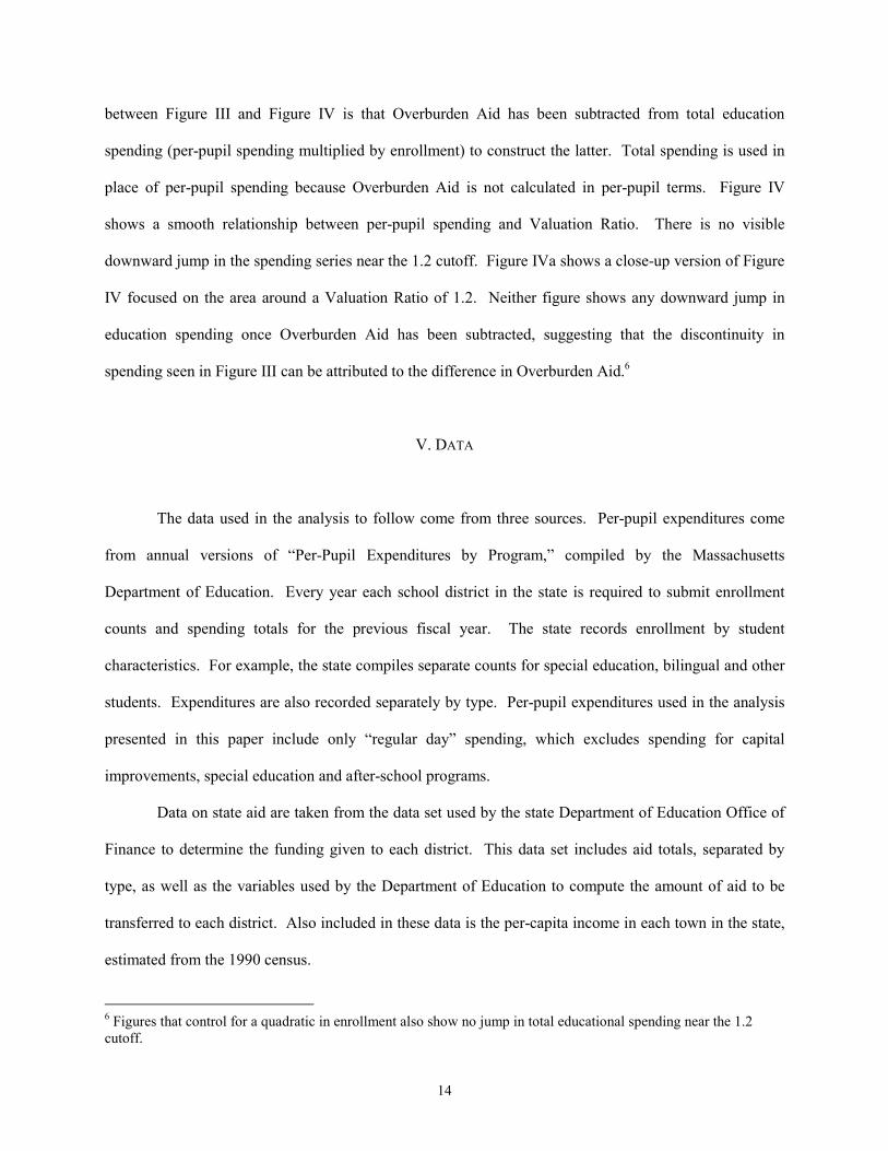
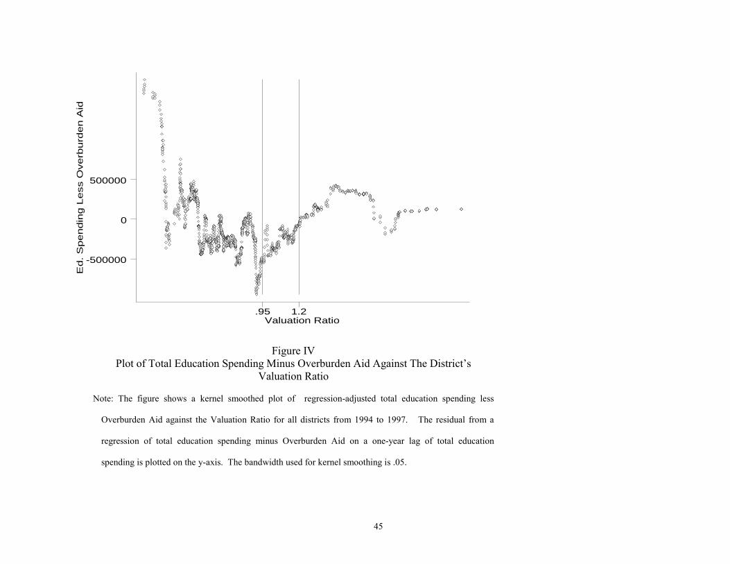
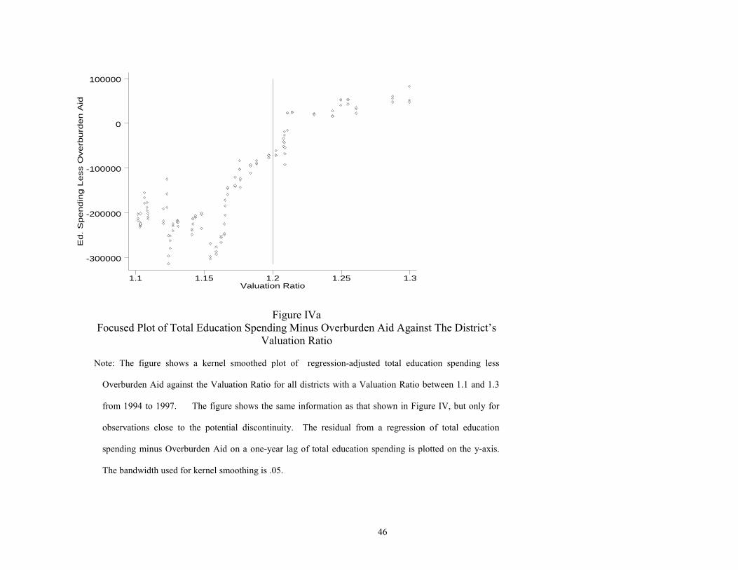
One way to test whether the discontinuity in spending at the 1.2 cutoff is due to the decline in

Overburden Aid is to produce a version of Figure III that does not include Overburden Aid. Figure IV

shows a plot of total education spending less Overburden Aid against Valuation Ratio. The difference

5 The bandwidth used in the figure is .05. The downward jump at 1.2 can be seen using bandwidths from .02 to .08.

Bandwidths greater than .08 smooth over the discontinuity, while bandwidths less than .02 leave too much variation

in spending to allow the naked eye to see the discontinuity.

14

between Figure III and Figure IV is that Overburden Aid has been subtracted from total education

spending (per-pupil spending multiplied by enrollment) to construct the latter. Total spending is used in

place of per-pupil spending because Overburden Aid is not calculated in per-pupil terms. Figure IV

shows a smooth relationship between per-pupil spending and Valuation Ratio. There is no visible

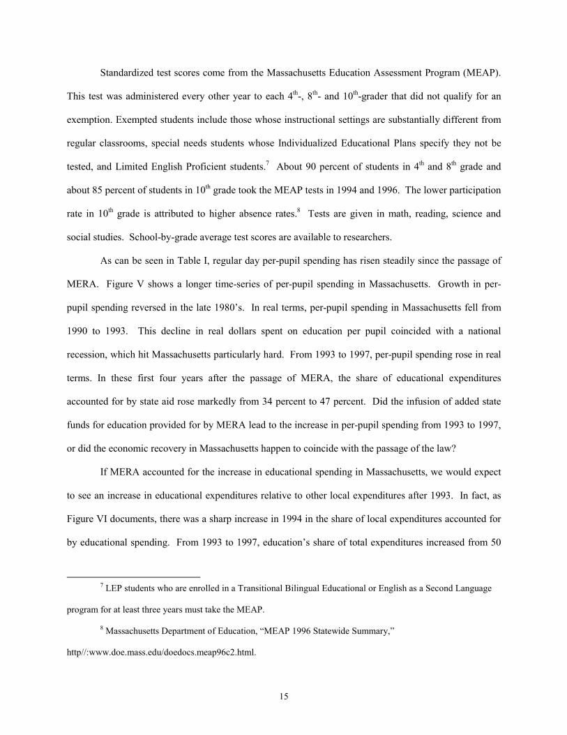
downward jump in the spending series near the 1.2 cutoff. Figure IVa shows a close-up version of Figure

IV focused on the area around a Valuation Ratio of 1.2. Neither figure shows any downward jump in

education spending once Overburden Aid has been subtracted, suggesting that the discontinuity in

spending seen in Figure III can be attributed to the difference in Overburden Aid.6

V. DATA

The data used in the analysis to follow come from three sources. Per-pupil expenditures come

from annual versions of Per-Pupil Expenditures by Program, compiled by the Massachusetts

Department of Education. Every year each school district in the state is required to submit enrollment

counts and spending totals for the previous fiscal year. The state records enrollment by student

characteristics. For example, the state compiles separate counts for special education, bilingual and other

students. Expenditures are also recorded separately by type. Per-pupil expenditures used in the analysis

presented in this paper include only regular day spending, which excludes spending for capital

improvements, special education and after-school programs.

Data on state aid are taken from the data set used by the state Department of Education Office of

Finance to determine the funding given to each district. This data set includes aid totals, separated by

type, as well as the variables used by the Department of Education to compute the amount of aid to be

transferred to each district. Also included in these data is the per-capita income in each town in the state,

estimated from the 1990 census.

6 Figures that control for a quadratic in enrollment also show no jump in total educational spending near the 1.2 cutoff.

15

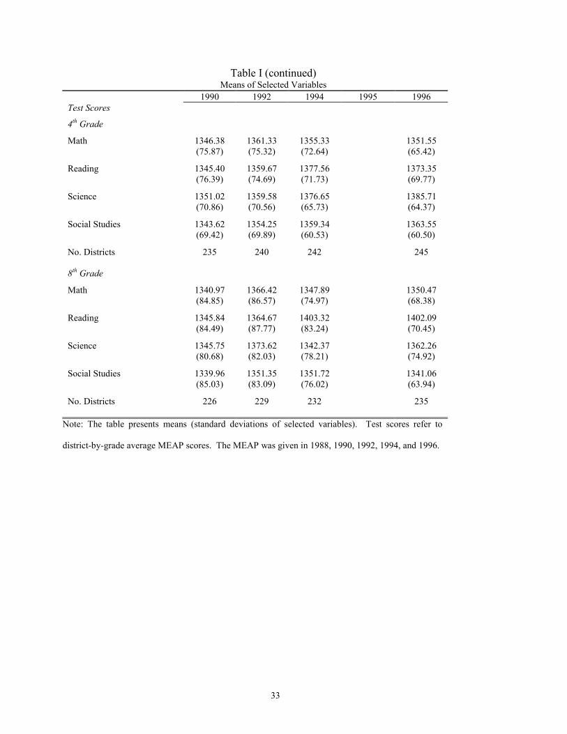
Standardized test scores come from the Massachusetts Education Assessment Program (MEAP).

This test was administered every other year to each 4th-, 8th- and 10th-grader that did not qualify for an

exemption. Exempted students include those whose instructional settings are substantially different from

regular classrooms, special needs students whose Individualized Educational Plans specify they not be

tested, and Limited English Proficient students.7 About 90 percent of students in 4th and 8th grade and

about 85 percent of students in 10th grade took the MEAP tests in 1994 and 1996. The lower participation

rate in 10th grade is attributed to higher absence rates.8 Tests are given in math, reading, science and

social studies. School-by-grade average test scores are available to researchers.

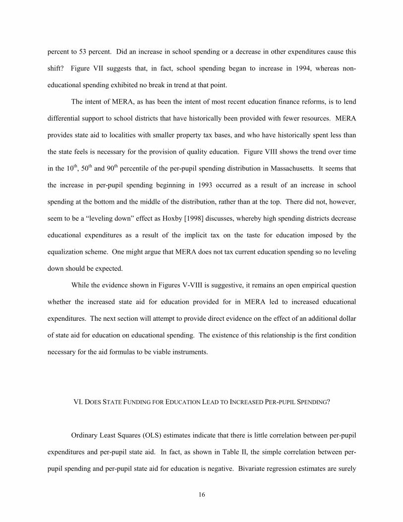
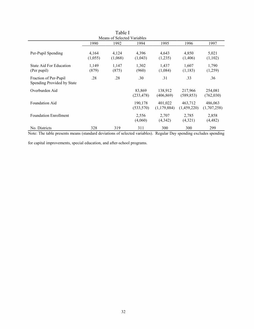
As can be seen in Table I, regular day per-pupil spending has risen steadily since the passage of

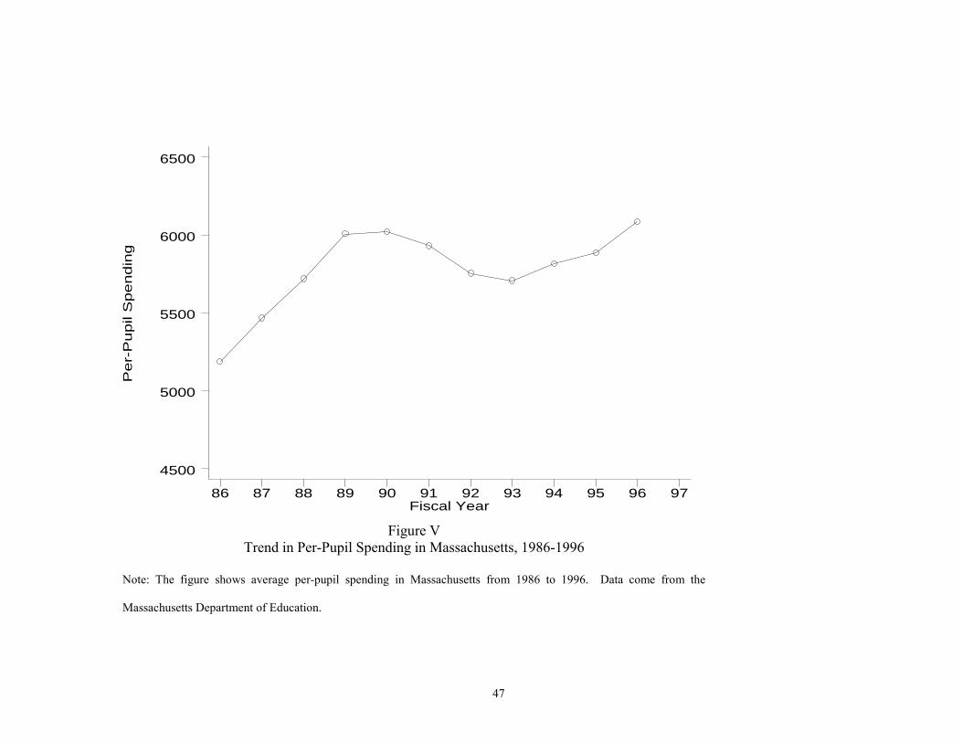
MERA. Figure V shows a longer time-series of per-pupil spending in Massachusetts. Growth in per-

pupil spending reversed in the late 1980s. In real terms, per-pupil spending in Massachusetts fell from

1990 to 1993. This decline in real dollars spent on education per pupil coincided with a national

recession, which hit Massachusetts particularly hard. From 1993 to 1997, per-pupil spending rose in real

terms. In these first four years after the passage of MERA, the share of educational expenditures

accounted for by state aid rose markedly from 34 percent to 47 percent. Did the infusion of added state

funds for education provided for by MERA lead to the increase in per-pupil spending from 1993 to 1997,

or did the economic recovery in Massachusetts happen to coincide with the passage of the law?

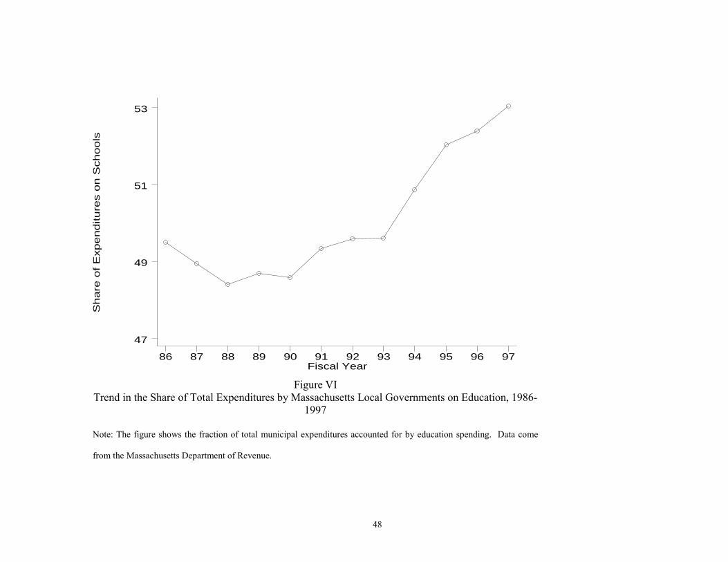
If MERA accounted for the increase in educational spending in Massachusetts, we would expect

to see an increase in educational expenditures relative to other local expenditures after 1993. In fact, as

Figure VI documents, there was a sharp increase in 1994 in the share of local expenditures accounted for

by educational spending. From 1993 to 1997, educations share of total expenditures increased from 50

7 LEP students who are enrolled in a Transitional Bilingual Educational or English as a Second Language

program for at least three years must take the MEAP.

8 Massachusetts Department of Education, MEAP 1996 Statewide Summary,

http//:www.doe.mass.edu/doedocs.meap96c2.html.

16

percent to 53 percent. Did an increase in school spending or a decrease in other expenditures cause this

shift? Figure VII suggests that, in fact, school spending began to increase in 1994, whereas non-

educational spending exhibited no break in trend at that point.

The intent of MERA, as has been the intent of most recent education finance reforms, is to lend

differential support to school districts that have historically been provided with fewer resources. MERA

provides state aid to localities with smaller property tax bases, and who have historically spent less than

the state feels is necessary for the provision of quality education. Figure VIII shows the trend over time

in the 10th, 50th and 90th percentile of the per-pupil spending distribution in Massachusetts. It seems that

the increase in per-pupil spending beginning in 1993 occurred as a result of an increase in school

spending at the bottom and the middle of the distribution, rather than at the top. There did not, however,

seem to be a leveling down effect as Hoxby [1998] discusses, whereby high spending districts decrease

educational expenditures as a result of the implicit tax on the taste for education imposed by the

equalization scheme. One might argue that MERA does not tax current education spending so no leveling

down should be expected.

While the evidence shown in Figures V-VIII is suggestive, it remains an open empirical question

whether the increased state aid for education provided for in MERA led to increased educational

expenditures. The next section will attempt to provide direct evidence on the effect of an additional dollar

of state aid for education on educational spending. The existence of this relationship is the first condition

necessary for the aid formulas to be viable instruments.

VI. DOES STATE FUNDING FOR EDUCATION LEAD TO INCREASED PER-PUPIL SPENDING?

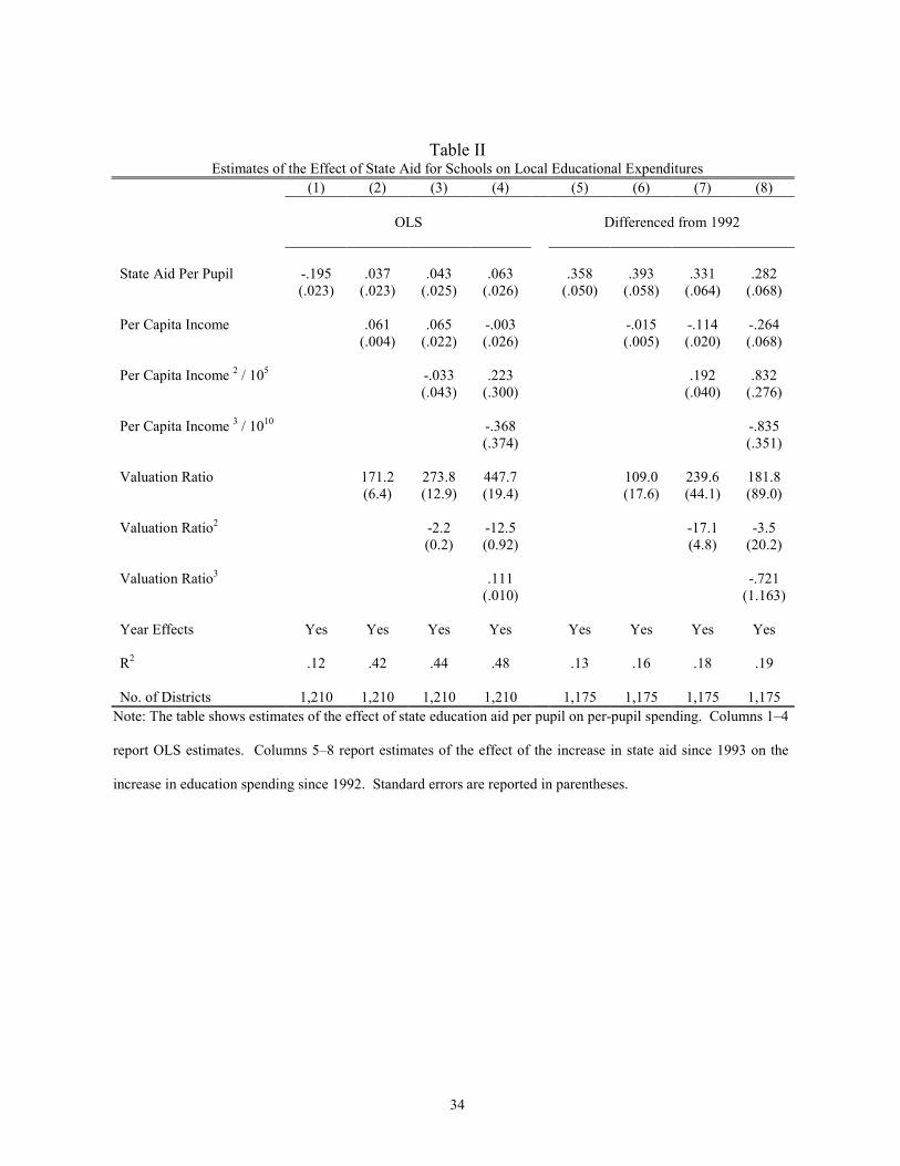
Ordinary Least Squares (OLS) estimates indicate that there is little correlation between per-pupil

expenditures and per-pupil state aid. In fact, as shown in Table II, the simple correlation between per-

pupil spending and per-pupil state aid for education is negative. Bivariate regression estimates are surely

17

biased, however, because state aid is mechanically negatively related to past per-pupil spending levels.

One strategy to produce better estimates is to control for economic characteristics of each school district

that characterize the districts ability to pay for education. Conditional on flexible functions of per-capita

income and the property tax base, state aid for education may no longer be related to past values of per-

pupil expenditures. As shown in Columns 24 of Table II, models that control for per-capita income and

for a measure of the property tax base produce estimates that are, in fact, more positive than those from

the bivariate regression (0.37 as compared to .195), but that are small in magnitude.

Controls for per-capita income and for measures of the property tax base may not solve the

inherent endogeneity problem, however. Tiebout sorting9 allows an individual to choose a level of public

good provision that suits his preferences. Conditional on wealth and income, an individual that has high

taste for education will choose to live in a school district with a higher implicit school tax rate. Since

state aid for education is systematically negatively related to taste for education, OLS estimates that

control for per-capita income and for a measure of the property tax base will also be biased downwards.

If differences in taste for education are fixed across school districts, measuring the effect of the change in

state aid for education on the change in per-pupil spending should yield better estimates.

A. Differencing Estimates of the Effect of State-Aid on Per-Pupil Spending

As shown in Columns 58 of Table II, estimates of the effect of a change in per-pupil state aid

since the passage of MERA on the change in per-pupil spending indicate a stronger effect of state aid.

Estimates are fairly precise and indicate that a one-dollar increase in state aid since 1993 is associated

with an increase in per-pupil spending of between 28 and 39 cents. The estimates are fairly insensitive to

polynomial controls for per-capita income and for a measure of the property tax base. These differencing

9 Tiebout, Charles M., A Pure Theory of Local Expenditures, Journal of Political Economy (October

1956) pp. 416-424.

18

estimates suggest that an increase in state aid for schools acts much as we might expect a lump sum grant

to a local municipality to act.

A simple benchmark is the assumption that localities have preferences that determine the share of

their budgets to devote to each category of expenditure; localities spend the marginal dollar at the same

proportion as they have spent on their total budgets. The underlying model in this case is, of course, not

general. The implication, however, is that relative to this benchmark the differencing estimates do not

suggest that there is any form of a fly-paper effect.

Differencing solves the problem that state aid is mechanically related to fixed characteristics of

school districts. However, if the change in state aid is related to determinants of per-pupil spending that

are not fixed across school districts, the estimates from differencing models will be biased. For example,

if the dispersion in per-pupil spending is growing over time, the change in state aid is negatively related to

1−− itit εε . In this case, the differencing strategy produces negatively biased estimates of the effect of a

change in state aid on the change in per-pupil spending.10

B. 2SLS Estimates of the Effect of State Aid on Per-Pupil Spending

Fortunately, MERA provides a potential solution to the endogeneity problem. As discussed in

Section III, the discontinuity of the formula used to determine Overburden Aid and the overweighting of

special education students in the formula used to determine Foundation Aid allow control for smooth

functions of per-capita income, a measure of the property tax base, and enrollment, while employing these

two state aid formulas as instruments for the change in state aid.

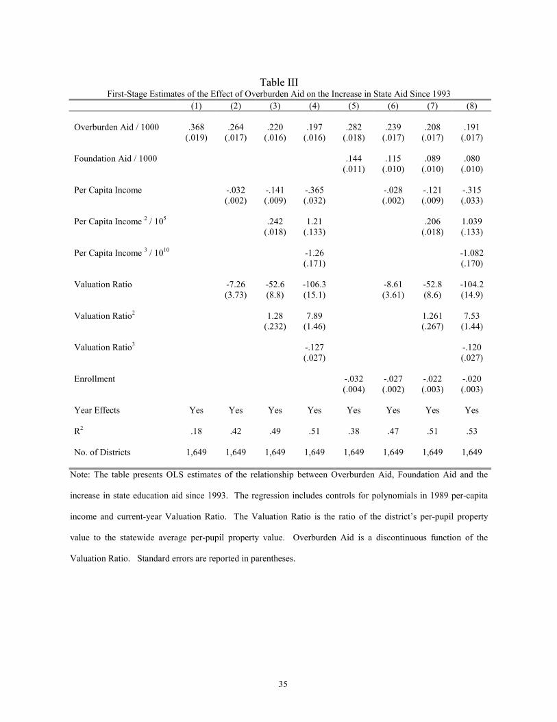
Estimates of the first-stage relationship, presented in Table III, indicate a strong association of

both types of aid with the increase in state aid since the passage of MERA. It is not surprising that

Overburden Aid is positively related to the increase in state aid. However, since Overburden Aid is

10 See Section III for a slightly more detailed explanation.

19

mainly a function of per-capita income and of the Valuation Ratio, the remaining correlation with the

increase in state aid is a result of the discontinuous nature of the Overburden Aid formula.

As shown in Columns 24 of Table III, increasingly flexible controls for per-capita income and

for a measure of the property tax base produce estimates of the relationship of Overburden Aid and the

increase in state aid that are progressively smaller in magnitude. The first-stage relationship remains

strong, even controlling for these flexible polynomial functions. Controlling for 3rd-order polynomials in

both per-capita income and a measure of the property tax base, the t-statistic on the effect of Overburden

Aid on the increase in state aid is greater than ten.

First-stage estimates, shown in Columns 58 of Table III, show that the relationship of both

Overburden Aid and Foundation Aid to the increase in state aid for schools is strong. Controlling for

polynomials in per-capita income and the Valuation Ratio and for Foundation Enrollment, the major

determinant of the Foundation Budget, both Overburden Aid and Foundation Aid are significantly

positively related to the increase in state aid for schools.

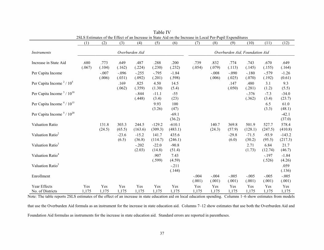
Two-stage least squares (2SLS) estimates of the effect of an increase in state aid for schools per

pupil on the increase in per-pupil expenditures are significantly larger than the differencing estimates

from Table II. As seen in Columns 1 and 2 of Table IV, models that employ Overburden Aid as an

instrument for the increase in state aid and control for up to a quadratic in per-capita income and the

Valuation Ratio suggest that about 65 cents of each dollar of state aid are spent on schools. Inclusion of

higher-order polynomials in per-capita income and the Valuation Ratio produce smaller estimates, which

are less precise and which look more like those from the differencing model (20 48 cents).

As compared with models that employ only Overburden Aid as an instrument for the increase in

state aid, those that use both Overburden Aid and Foundation Aid as instruments provide estimates that

are more precise and larger in magnitude. Presented in Columns 712 of Table IV, these models control

for Foundation Enrollment as well as the usual polynomials in per-capita income and the Valuation Ratio.

Estimates of the effect of a dollar per pupil increase in state aid on per-pupil expenditures range from 65

cents to 83 cents. The estimates are fairly precise, although the smaller estimates cannot rule out the

20

possibility that the differencing estimates from Table II are correct. On the whole, however, 2SLS

estimates seem to suggest that the differencing estimates are too small. It seems that municipalities in

Massachusetts spent more than 50 cents and maybe up to 75 cents of each dollar of state aid for education

on the schools.

One should also note that the estimates produced by the 2SLS estimation strategy are remarkably

similar to the estimate produced by the graphical analysis in Section IV. The graphical analysis pointed

out that Figure III reveals a marked drop in per-pupil spending at a Valuation Ratio of 1.2 the point

where Overburden Aid goes to zero. This decline in per-pupil spending is about $90. The average award

of Overburden Aid from 1994 to 1997 for districts with a positive Standard of Effort Gap was $163 per

pupil. Thus, the regression-discontinuity analysis suggests that each dollar of Overburden Aid translates

into about 55 cents of additional educational expenditures. This estimate falls within the range of the

2SLS estimates.

VII. DOES MONEY MATTER?

The estimates presented in Section VI show that increased state education aid induces increased

per-pupil expenditures. The results show that conditional on smooth functions of the Valuation Ratio,

per-capita income, and enrollment the Overburden Aid and Foundation Aid formulas have predictive

power for per-pupil spending. Thus, the aid formulas can be used as instruments for education spending

to estimate the effect of per-pupil spending on student achievement.

A. Estimates of the Effect of Increased Per-pupil Spending on the Increase in Test Scores

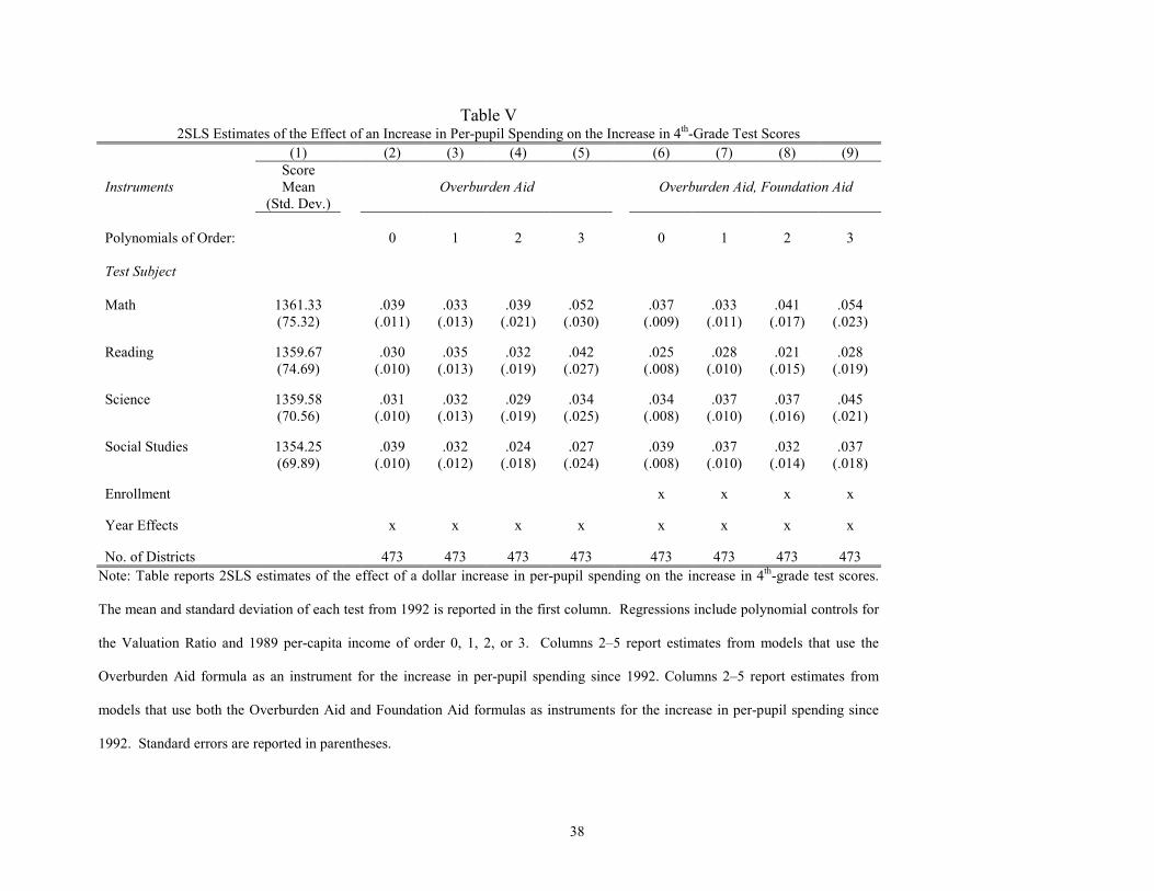
Tables V and VI present estimates from models that use Overburden Aid and Foundation Aid as

instruments for the increase in per-pupil spending since 1992. Estimates for 4th-grade test scores are

21

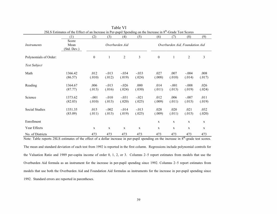
shown in Table V, while estimates for 8th-graders are shown in Table VI. The estimates suggest that a

plausibly exogenous increase in per-pupil spending leads to an increase in 4th-grade test scores. Estimates

for 8th-graders show no evidence of an effect of spending on average test scores.

Estimated effects for 4th-grade test scores are nearly all significantly different from zero, and

remain remarkably consistent across specifications and across test subjects. Inclusion of higher-order

polynomials in the Valuation Ratio and per-capita income does not seem to have a monotonic effect on

the estimated coefficient. Across test subjects, specifications that include 3rd-order polynomials produce

estimates that are mostly insignificantly different from zero, but these point estimates are almost

uniformly greater in magnitude than those from other specifications. Specifications that use both

Overburden Aid and Foundation Aid as instruments yield more precise, but not significantly different,

estimates than those that only use Overburden Aid. In short, estimated effects on 4th-grade test scores are

fairly robust to specification changes.

Estimated magnitudes are fairly large. The median estimate from Table V (.034) implies that a

one standard deviation increase in per-pupil spending ($1,000) leads to a 34-point increase in 4th-grade

test scores. This increase is about as large as one-half of a standard deviation in district average test

scores.

In contrast, estimates for 8th-graders show no evidence that increases in per-pupil spending had

any effect on test scores. Point estimates are both positive and negative; few specifications produce

estimates that are statistically significantly different from zero. Furthermore, controlling for higher-order

polynomials leads to estimates of the effect of per-pupil spending on 8th-grade test scores that flip from

negative to positive, and back again. Based on the results shown in Table VI, there does not seem to be

any evidence that increases in per-pupil spending had any effect on 8th-grade test scores.

B. Effects on the Quantiles of the Test-score Distribution

Most existing studies of school inputs effect on student achievement focus on the effect on mean

test scores. There is reason to believe that changes in inputs may have varying effects on students at

22

different points in the test-score distribution. These effects may be masked when looking at test-score

means. For example, consider the case where increased resources are used to buy lab equipment, or

computers, that are skill-complementary. As a result, math and science test scores increase for the best

students. But, the resulting substitution of the teachers time away from skill-substitute teaching efforts

lead to a decrease in math and science test scores among low-scoring students. The resulting effect on

mean test scores is ambiguous, and may be zero. However, in this example money has a real effect on

students test scores. The example could also work in the opposite direction. Consider the case where

additional educational funds are spent on remedial teaching materials. Low-scoring students benefit, and

high-scoring students suffer as the teacher spends time teaching the weaker students. The effect on mean

test scores is again ambiguous.

The reported MEAP scores used in this study provide a chance to examine effects at additional

points of the test score distribution. For each observation, the data report the fraction of students

performing at each of five proficiency levels: below level 1, at level 1, at level 2, at level 3, and at level 4.

Students at level 1 should be beginning to grasp factual knowledge. Students at level 2 should have a

firm grasp of factual knowledge. Students at level 3 should be beginning to think critically, problem-

solve, reason and communicate effectively. And students at level 4 should exhibit exemplary

knowledge, thinking, reasoning, and communication skills.11

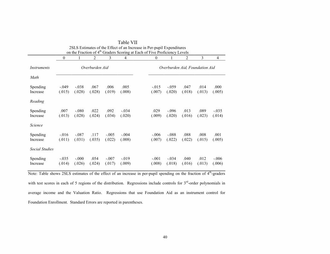
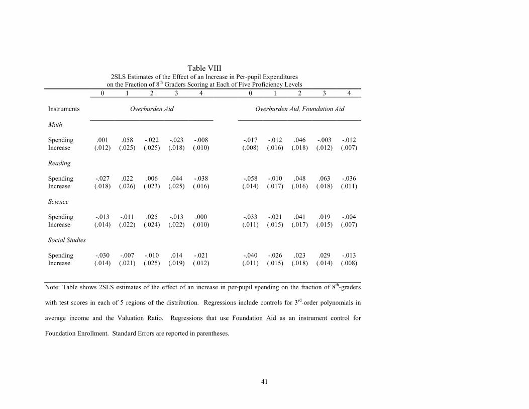
Tables VII and VIII present results from models that estimate the effect of an increase in per-

pupil spending on the increase in the fraction of students scoring at each proficiency level. Results for 4th

graders are presented in Table VII and in Figures IXa and IXb. Table VII shows 2SLS estimates of the

effect of an increase in per-pupil spending on the fraction of 4th graders scoring at each of the five

proficiency levels. Figures IXaIXb show the effect on the 4th-grade test score distribution of a $1000 per

pupil increase in educational spending. The results generally suggest that 4th-grade mean test score

11 Massachusetts Department of Education, MEAP 1996 Statewide Summary,

http//:www.doe.mass.edu/doedocs.meap96c2.html.

23

increases came as a result of a decrease in the fraction of students scoring at level 1 and an increase in the

fraction of students scoring at level 2 or 3.

In math, science, and social studies, most of the increase in test score means induced by increased

funding came as a result of movement at the bottom of the test score distribution. In these three subjects,

increases in per-pupil spending seem to have led to a decrease in the fraction of students scoring at level 1

and an increase in the fraction of students scoring at level 2. In reading, increases in mean test scores

seem to have come as a result of a decrease in the fraction of students scoring at level 1 and an increase in

the fraction of students scoring at level 3. These results suggest that increased funding affected a wider

range of the reading test score distribution than the math, science, or social studies distributions.

The results for 8th graders are less clear. Far fewer of the estimated effects of per-pupil spending,

presented in Table VIII, are significantly different from zero. As shown in Figures Xa and Xb, increased

educational funding seems to have led to a decrease in the fraction of 8th graders scoring at both tails of

the test score distribution. However, it is not clear what effect, if any, increased school spending had on

the middle of the distribution of 8th-grade test scores. The finding that increases in funding led to a

decrease in students scoring both below level 1 and at level 4 is consistent with schools using added

resources on teaching goods that are gross substitutes for students learning ability. In fact, the findings

for both 4th and 8th graders are consistent with the hypothesis that added resources are targeted towards

helping low-achieving students. However, if this hypothesis is to fit the empirical estimates in this paper,

the increased attention paid to weaker students must harm high-achieving 8th-graders more than it harms

high-achieving 4th-graders.

In light of the fact that 8th-grade classrooms are more likely than 4th-grade classrooms to be

homogeneously grouped by ability, it may seem unlikely that actions that affect low-achieving students

would have a larger negative effect on high-achieving 8th graders than on high-achieving 4th-graders.

However, teaching practices12 in the 4th grade may be more complementary across student skill groups

12 By teaching practices I mean any use of educational expenditures aimed at helping students to learn.

24

than in the 8th grade. It is possible that because the material taught in 4th-grade is based less on

cumulative knowledge, teaching efforts aimed at struggling students have a more beneficial effect on the

learning of the rest of the classroom in 4th grade than in 8th grade.

VIII. CONCLUSIONS

Since the release of the Coleman Report in 1966, and probably earlier, economists and

policymakers have debated whether added resources make schools more effective. The question of

whether increased funding of schools leads to improved student achievement remains controversial

mainly because the observed relationship between spending and test scores is driven partly by district

characteristics other than per-pupil spending. As I have shown, this endogeneity problem can be solved

using the idiosyncratic variation in spending created by recent equalization schemes. Equalization

schemes attempt to decrease within-state inequality in per-pupil spending by giving more state education

aid to districts that historically have spent less on schools.

In this paper, I use the discontinuous aid formula provided by the Massachusetts Education

Reform Act of 1993 (MERA) to identify the effect of increased per-pupil spending on student test scores.

MERA redistributes education funding across districts using information on past spending levels, student

characteristics, property values, and per-capita income. I use the MERA aid formula as an instrument for

the increase in per-pupil spending to estimate the effect of spending on test scores. A graphical analysis

illustrates that the variation in spending used in the estimation comes from the discontinuity of the aid

formula.

The estimates suggest that spending increases do lead to improved test scores. Estimates for 4th-

graders suggest that a one standard deviation increase in per-pupil spending ($1000) increases math,

reading, science and social studies test scores by about a half of a standard deviation. Nearly all estimates

are significantly different from zero. Estimated effects are remarkably consistent across specifications

and test subjects. Estimates for 8th-graders show no evidence of an effect of spending on district average

25

test scores. One explanation for the difference between 4th- and 8th-grade effects is that 4th-graders spent a

larger fraction of their education in well-funded schools. This explanation is buttressed by the

observation that MERA bases funding partly on fixed district characteristics, so the same districts tend to

receive funding each year.

Further investigation into the effects of spending on the distribution of test scores suggests that

increases in 4th-grade test scores come as a result of an increase in performance by students at the bottom

of the distribution. The results also suggest that increases in spending led to a decrease in the fraction of

8th-graders scoring at both ends of the distribution. Future work should investigate possible explanations

for this finding.

26

REFERENCES

Angrist, Joshua D. and Alan B. Krueger, Empirical Strategies in Labor Economics, MIT Department of

Economics Working Paper (October 1998).

_____, and Victor Lavy, Does Teacher Training Affect Pupil Learning? Evidence from Matched

Comparisons in Jerusalem Public Schools, NBER Working Paper No. 6781 (November 1998).

_____, and _____, Using Maimonides Rule to Estimate the Effect of Class Size on Scholastic

Achievement, Quarterly Journal of Economics, CXIV (1999), 533-575.

Betts, Julian, Does School Quality Matter? Evidence from the National Longitudinal Survey of Youth,

Review of Economics and Statistics, LXXVII (1995), 231-250.

Bradbury, Katharine L., Christopher J. Mayer, and Karl E. Case, Property Tax Limits and Local Fiscal

Behavior: Did Massachusetts Cities and Towns Spend Too Little on Town Services under

Proposition 2 1/2? Federal Reserve Bank of Boston Working Paper, XCVII (February 1997).

Campbell, Donald and Julian Stanley, Experimental and Quasi-experimental Designs for Research

(Chicago, IL: Rand McNally College Publishing Company, 1963).

Card, David and Alan Krueger, Does School Quality Matter? Returns to Education and the

Characteristics of Public Schools in the United States, Journal of Political Economy, C

(February 1992) 1-40.

27

_____, and _____, School Resources and Student Outcomes: An Overview of the Literature and New

Evidence from North and South Carolina, Journal of Economic Perspectives, X (Fall 1996) 31-

50.

_____, and Abigail Payne, School Finance Reform, the Distribution of School Spending, and the

Distribution of SAT Scores, Princeton University Industrial Relations Section Working Paper

#387 (July 1997).

Clinton, William J., State of the Union Address (January 27, 2000).

Coleman, James S., Equality of Educational Opportunity, (Washington, D.C.: U. S. Department of

Health, Education, and Welfare, 1966).

Craig, Steven G. and Robert P. Inman, Federal Aid and Public Education: An Empirical Look at the

New Fiscal Federalism, Review of Economics and Statistics, LXIV (November 1982) 541-552.

Cullen, Julie Essays on Special Education Finance and Intergovernmental Relations Ph.D. Dissertation

M.I.T. Department of Economics (May 1997).

Cutler, David M., Douglas W. Elmendorf and Richard Zeckhauser, Restraining the Leviathan: Property

Tax Limitation in Massachusetts, Journal of Public Economics, LXXI (March 1999) 313-34.

Downes, Thomas Evaluating the Impact of School Finance Reform on the Provision of Public

Education: The California Case National Tax Journal, XLV (December 1992) 405-419.

28

Duflo, Esther, Schooling and Labor Market Consequences of School Construction in Indonesia:

Evidence from and Unusual Policy Experiment, MIT mimeo (1999).

Duggan, Mark G., Hospital Ownership and Public Medical Spending, NBER Working Paper No. 7789

(July 2000).

Ehrenberg, Ronald G. and Dominic J. Brewer, Do School and Teacher Characteristics Matter? Evidence

from High School and Beyond, Economics of Education Review, XIII (1994) 1-17.

Feldstein, Martin, The Effect of a Differential Add-On Grant: Title I and Local Education Spending,

Journal of Human Resources, XIII (Fall 1978) 443-458.

Fernandez, Raquel, Education Finance Reform and Investment in Human Capital: Lessons from

California, Journal of Public Economics, LXXIV (December 1999) 327-350.

Flyer, Frederick and Sherwin Rosen, The New Economics of Teachers and Education, Journal of Labor

Economics, XV (1997) S104-S139.

Hanushek, Eric A., The Economics of Schooling: Production and Efficiency in Public Schools, Journal

of Economic Literature XXIV (September 1986) 1141-1177.

_____, Teacher Characteristics and Gains in Student Achievement: Estimation Using Micro Data,

American Economic Review, LXI (1971) 280-288.

_____, Steven Rivkin, and John Kain, Teachers, Schools and Academic Achievement, mimeo. (1998).

29

Heckman, James J., Sample Selection Bias as a Specification Error, Econometrica, XLVII (January

1979) 153-161.

_____, Robert J. LaLonde, and Jeffrey A. Smith, The Economics and Econometrics of Active Labor

Market Programs, Handbook of Labor Economics, Vol. III, Orley Ashenfelter and David Card

eds. (Amsterdam: Elsevier Science, North-Holland Publishers, 1999).

_____, Anne Layne-Farrar, and Petra Todd, Does Measured School Quality Really Matter? An

Examination of the Earnings-Quality Relationship, Does Money Matter? The Effect of School

Resources on Student Achievement and Adult Success, Gary Burtless ed. (Washington D.C.:

Brookings Institution Press, 1996) 192-289.

Hedges, Larry V., R. D. Laine, and R. Greenwald, Does Money Matter? A Meta-Analysis of Studies of

the Effects of Differential School Inputs on Student Outcomes, Educational Researcher, XXIII

(1994) 5-14.

Hoxby, Caroline, All School Finance Equalizations Are Not Created Equal, mimeo. (May 1998).

Hoxby, Caroline, The Effects of Class Size and Composition on Student Achievement: New Evidence

from Natural Population Variation, mimeo. (July 1996).

_____, Are Efficiency and Equity in School Finance Substitutes or Complements? Journal of Economic

Perspectives, X (Fall 1996) 51-72.

Imbens, Guido, Jeffrey B. Liebman, and Nada Eissa, The Econometrics of Difference in Differences,

mimeo (January 1997).

30

Krueger, Alan B., Experimental Estimates of Education Production Functions, Quarterly Journal of

Economics, CXIV (May 1999) 497-532.

Krugman, Paul, The Age of Diminished Expectations: U.S. Economic policy in the 1990s, (Cambridge,

MA: MIT Press, 1994).

Loeb, Susanna and John Bound, The Effect of Measured School Inputs on Academic Achievement:

Evidence from the 1920s, 1930s and 1940s Birth Cohorts, Review of Economics and

Statistics, LXXVIII (November 1996) 653-664.

Massachusetts Municipal Profiles, Edith R. Hornor ed. (Palo Alto, CA: Information Publications, 1988-

1996).

Murray, Sheila, William Evans and Robert Schwab, Education-Finance Reform and the Distribution of

Education Resources, American Economic Review, LXXXVIII (September 1998) 789-812.

Peltzman, Sam, The Political Economy of the Decline of American Public Education, Journal of Law

and Economics, XXXVI (April 1993) 331-370.

_____, Political Economy of Public Education: Non-College-Bound Students, Journal of Law and

Economics, XXXIX (April 1996) 73-120.

Psacharopoulos, George, The Contribution of Education to Economic Growth: International

Comparisons, International Comparisons of Productivity and Causes of the Slowdown, John W.

Kendrick ed. (Cambridge, MA: Ballinger Publishing Co., 1984) 335-355.

31

Schultz, Theodore W., Education and Economic Growth, Social Forces Influencing American

Education, N.B. Henry ed. (Chicago, IL: University of Chicago Press, 1961) 46-88.

_____, Nobel Lecture: The Economics of Being Poor, Journal of Political Economy, LXXXVIII

(August 1980) 639-651.

Tiebout, Charles M., A Pure Theory of Local Expenditures, Journal of Political Economy, LXIV

(October 1956) 416-424.

Trochim, William, Research Design for Program Evaluation: The Regression Discontinuity Approach,

(Beverly Hills, CA: Sage Publications, 1984).

van der Klaauw, Wilbert, A Regression-Discontinuity Evaluation of the Effect of

Financial Aid Offers on College Enrollment mimeo. (December 1996).

32

Table I Means of Selected Variables

1990 1992 1994 1995 1996 1997 Per-Pupil Spending

4,164 (1,055)

4,124 (1,068)

4,396 (1,043)

4,643 (1,235)

4,850 (1,406)

5,021 (1,102)

State Aid For Education (Per pupil)

1,149 (879)

1,147 (875)

1,302 (960)

1,437 (1,084)

1,607 (1,183)

1,790 (1,259)

Fraction of Per-Pupil Spending Provided by State

.28 .28 .30 .31 .33 .36

Overburden Aid

83,869 (233,478)

138,912 (406,869)

217,966 (589,853)

254,081 (762,030)

Foundation Aid 190,178 (533,570)

401,022 (1,179,884)

463,712 (1,459,220)

486,063 (1,707,258)

Foundation Enrollment 2,556 (4,060)

2,707 (4,342)

2,785 (4,321)

2,858 (4,482)

No. Districts 328 319 311 300 300 299 Note: The table presents means (standard deviations of selected variables). Regular Day spending excludes spending

for capital improvements, special education, and after-school programs.

33

Table I (continued) Means of Selected Variables

1990 1992 1994 1995 1996 Test Scores

4th Grade

Math

1346.38 (75.87)

1361.33 (75.32)

1355.33 (72.64)

1351.55 (65.42)

Reading

1345.40 (76.39)

1359.67 (74.69)

1377.56 (71.73)

1373.35 (69.77)

Science

1351.02 (70.86)

1359.58 (70.56)

1376.65 (65.73)

1385.71 (64.37)

Social Studies

1343.62 (69.42)

1354.25 (69.89)

1359.34 (60.53)

1363.55 (60.50)

No. Districts

235 240 242 245

8th Grade

Math

1340.97 (84.85)

1366.42 (86.57)

1347.89 (74.97)

1350.47 (68.38)

Reading

1345.84 (84.49)

1364.67 (87.77)

1403.32 (83.24)

1402.09 (70.45)

Science

1345.75 (80.68)

1373.62 (82.03)

1342.37 (78.21)

1362.26 (74.92)

Social Studies

1339.96 (85.03)

1351.35 (83.09)

1351.72 (76.02)

1341.06 (63.94)

No. Districts

226 229 232 235

Note: The table presents means (standard deviations of selected variables). Test scores refer to

district-by-grade average MEAP scores. The MEAP was given in 1988, 1990, 1992, 1994, and 1996.

34

Table II Estimates of the Effect of State Aid for Schools on Local Educational Expenditures

(1) (2) (3) (4) (5) (6) (7) (8)

OLS

Differenced from 1992

State Aid Per Pupil -.195

(.023)

.037 (.023)

.043 (.025)

.063 (.026)

.358 (.050)

.393 (.058)

.331 (.064)

.282 (.068)

Per Capita Income .061 (.004)

.065 (.022)

-.003 (.026)

-.015 (.005)

-.114 (.020)

-.264 (.068)

Per Capita Income 2 / 105 -.033 (.043)

.223 (.300)

.192 (.040)

.832 (.276)

Per Capita Income 3 / 1010

-.368

(.374)

-.835 (.351)

Valuation Ratio 171.2 (6.4)

273.8 (12.9)

447.7 (19.4)

109.0 (17.6)

239.6 (44.1)

181.8 (89.0)

Valuation Ratio2 -2.2 (0.2)

-12.5 (0.92)

-17.1 (4.8)

-3.5 (20.2)

Valuation Ratio3 .111 (.010)

-.721 (1.163)

Year Effects Yes

Yes Yes Yes Yes

Yes Yes Yes

R2 .12

.42 .44 .48 .13 .16 .18 .19

No. of Districts 1,210 1,210 1,210 1,210 1,175 1,175 1,175 1,175 Note: The table shows estimates of the effect of state education aid per pupil on per-pupil spending. Columns 14

report OLS estimates. Columns 58 report estimates of the effect of the increase in state aid since 1993 on the

increase in education spending since 1992. Standard errors are reported in parentheses.

35

Table III

First-Stage Estimates of the Effect of Overburden Aid on the Increase in State Aid Since 1993 (1) (2) (3) (4) (5) (6) (7) (8) Overburden Aid / 1000 .368

(.019)

.264 (.017)

.220 (.016)

.197 (.016)

.282 (.018)

.239 (.017)

.208 (.017)

.191 (.017)

Foundation Aid / 1000 .144 (.011)

.115 (.010)

.089 (.010)

.080 (.010)

Per Capita Income -.032 (.002)

-.141 (.009)

-.365 (.032)

-.028 (.002)

-.121 (.009)

-.315 (.033)

Per Capita Income 2 / 105 .242 (.018)

1.21 (.133)

.206 (.018)

1.039 (.133)

Per Capita Income 3 / 1010 -1.26 (.171)

-1.082 (.170)

Valuation Ratio -7.26 (3.73)

-52.6 (8.8)

-106.3 (15.1)

-8.61 (3.61)

-52.8 (8.6)

-104.2 (14.9)

Valuation Ratio2 1.28 (.232)

7.89 (1.46)

1.261 (.267)

7.53 (1.44)

Valuation Ratio3 -.127 (.027)

-.120 (.027)

Enrollment -.032 (.004)

-.027 (.002)

-.022 (.003)

-.020 (.003)

Year Effects Yes

Yes Yes Yes Yes Yes Yes Yes

R2 .18

.42 .49 .51 .38 .47 .51 .53

No. of Districts 1,649 1,649 1,649 1,649 1,649 1,649 1,649 1,649

Note: The table presents OLS estimates of the relationship between Overburden Aid, Foundation Aid and the

increase in state education aid since 1993. The regression includes controls for polynomials in 1989 per-capita

income and current-year Valuation Ratio. The Valuation Ratio is the ratio of the districts per-pupil property

value to the statewide average per-pupil property value. Overburden Aid is a discontinuous function of the

Valuation Ratio. Standard errors are reported in parentheses.

37

Table IV 2SLS Estimates of the Effect of an Increase in State Aid on the Increase in Local Per-Pupil Expenditures

(1) (2) (3) (4) (5) (6) (7) (8) (9) (10) (11) (12) Instruments

Overburden Aid

Overburden Aid, Foundation Aid

Increase in State Aid .680

(.067) .773

(.104) .649

(.162) .487

(.224) .288

(.230) .200

(.232) .739

(.054) .832

(.079) .774

(.113) .743

(.145) .670

(.155) .649

(.164) Per Capita Income -.007

(.006) -.096 (.031)

-.255 (.092)

-.795 (.201)

-1.84 (.598)

-.008 (.006)

-.090 (.025)

-.180 (.070)

-.579 (.192)

-1.26 (0.61)

Per Capita Income 2 / 105 .169 (.062)

.825 (.359)

4.50 (1.30)

14.5 (5.4)

.147 (.050)

.480 (.281)

3.1 (1.2)

9.3 (5.5)

Per Capita Income 3 / 1010 -.844 (.448)

-11.1 (3.4)

-55 (23)

-.376 (.362)

-7.3 (3.4)

-34.0 (23.7)

Per Capita Income 4 / 1015 9.93 (3.26)

100 (47)

6.5 (3.3)

61.0 (48.1)

Per Capita Income 5 / 1020 -69.1 (36.2)

-42.1 (37.0)

Valuation Ratio 131.8 (24.5)

303.3 (65.5)

244.5 (163.6)

-129.2 (309.3)

-610.1 (483.1)

140.7 (24.3)

369.8 (57.9)

501.9 (128.1)

527.7 (247.5)

578.4 (410.8)

Valuation Ratio2 -23.6 (6.5)

-15.2 (36.8)

141.7 (114.7)

435.6 (246.1)

-29.8 (6.0)

-71.5 (30.2)

-93.9 (95.5)

-143.2 (217.3)

Valuation Ratio3 -.202 (2.03)

-22.0 (14.8)

-90.8 (51.4)

2.71 (1.73)

6.84 (12.74)

21.7 (46.7)

Valuation Ratio4 .907 (.599)

7.43 (4.59)

-.197 (.526)

-1.84 (4.26)

Valuation Ratio5 -.211 (.144)

.059 (.136)

Enrollment -.004 (.001)

-.004 (.001)

-.005 (.001)

-.005 (.001)

-.005 (.001)

-.005 (.001)

Year Effects Yes Yes Yes Yes Yes Yes Yes Yes Yes Yes Yes Yes No. of Districts 1,175 1,175 1,175 1,175 1,175 1,175 1,175 1,175 1,175 1,175 1,175 1,175

Note: The table reports 2SLS estimates of the effect of an increase in state education aid on local education spending. Columns 16 show estimates from models

that use the Overburden Aid formula as an instrument for the increase in state education aid. Columns 712 show estimates that use both the Overburden Aid and

Foundation Aid formulas as instruments for the increase in state education aid. Standard errors are reported in parentheses.

38

Table V 2SLS Estimates of the Effect of an Increase in Per-pupil Spending on the Increase in 4th-Grade Test Scores

(1) (2) (3) (4) (5) (6) (7) (8) (9) Instruments

Score Mean

(Std. Dev.)

Overburden Aid


Polynomials of Order: 0 1 2 3 0 1 2 3 Test Subject

Math 1361.33 (75.32)

.039 (.011)

.033 (.013)

.039 (.021)

.052 (.030)

.037 (.009)

.033 (.011)

.041 (.017)

.054 (.023)

Reading 1359.67 (74.69)

.030 (.010)

.035 (.013)

.032 (.019)

.042 (.027)

.025 (.008)

.028 (.010)

.021 (.015)

.028 (.019)

Science 1359.58 (70.56)

.031 (.010)

.032 (.013)

.029 (.019)

.034 (.025)

.034 (.008)

.037 (.010)

.037 (.016)

.045 (.021)

Social Studies 1354.25 (69.89)

.039 (.010)

.032 (.012)

.024 (.018)

.027 (.024)

.039 (.008)

.037 (.010)

.032 (.014)

.037 (.018)

Enrollment x x x x

Year Effects x x x x x x x x

No. of Districts 473 473 473 473 473 473 473 473 Note: Table reports 2SLS estimates of the effect of a dollar increase in per-pupil spending on the increase in 4th-grade test scores.

The mean and standard deviation of each test from 1992 is reported in the first column. Regressions include polynomial controls for

the Valuation Ratio and 1989 per-capita income of order 0, 1, 2, or 3. Columns 25 report estimates from models that use the

Overburden Aid formula as an instrument for the increase in per-pupil spending since 1992. Columns 25 report estimates from

models that use both the Overburden Aid and Foundation Aid formulas as instruments for the increase in per-pupil spending since

1992. Standard errors are reported in parentheses.

39

Table VI 2SLS Estimates of the Effect of an Increase in Per-pupil Spending on the Increase in 8th-Grade Test Scores

(1) (2) (3) (4) (5) (6) (7) (8) (9) Instruments

Score Mean

(Std. Dev.)

Overburden Aid


Polynomials of Order: 0 1 2 3 0 1 2 3 Test Subject

Math 1366.42 (86.57)

.012 (.010)

-.013 (.012)

-.034 (.019)

-.033 (.024)

.027 (.008)

.007 (.010)

-.004 (.014)

.008 (.017)

Reading 1364.67 (87.77)

.006 (.013)

-.013 (.016)

-.026 (.024)

.000 (.030)

.014 (.011)

-.001 (.013)

-.008 (.019)

.026 (.024)

Science 1373.62 (82.03)

-.001 (.010)

-.010 (.013)

-.031 (.020)

-.021 (.025)

.012 (.009)

.006 (.011)

-.007 (.015)

.011 (.019)

Social Studies 1351.35 (83.09)

.015 (.011)

-.002 (.013)

-.014 (.019)

-.013 (.025)

.028 (.009)

.020 (.011)

.021 (.015)

.032 (.020)

Enrollment x x x x

Year Effects x x x x x x x x

No. of Districts 473 473 473 473 473 473 473 473 Note: Table reports 2SLS estimates of the effect of a dollar increase in per-pupil spending on the increase in 8th-grade test scores.

The mean and standard deviation of each test from 1992 is reported in the first column. Regressions include polynomial controls for

the Valuation Ratio and 1989 per-capita income of order 0, 1, 2, or 3. Columns 25 report estimates from models that use the

Overburden Aid formula as an instrument for the increase in per-pupil spending since 1992. Columns 25 report estimates from

models that use both the Overburden Aid and Foundation Aid formulas as instruments for the increase in per-pupil spending since

1992. Standard errors are reported in parentheses.

40

Table VII 2SLS Estimates of the Effect of an Increase in Per-pupil Expenditures

on the Fraction of 4th Graders Scoring at Each of Five Proficiency Levels 0 1 2 3 4 0 1 2 3 4 Instruments

Overburden Aid


Math

Spending Increase

-.049 (.015)

-.038 (.028)

.067 (.028)

.006 (.019)

.005 (.008)

-.015 (.007)

-.059 (.020)

.047 (.018)

.014 (.013)

.000 (.005)

Reading

Spending Increase

.007 (.013)

-.080 (.028)

.022 (.024)

.092 (.034)

-.034 (.020)

.029 (.009)

-.096 (.020)

.013 (.016)

.089 (.023)

-.035 (.014)

Science

Spending Increase

-.016 (.011)

-.087 (.031)

.117 (.035)

-.005 (.022)

-.004 (.008)

-.006 (.007)

-.088 (.022)

.088 (.022)

.008 (.015)

.001 (.005)

Social Studies

Spending Increase

-.035 (.014)

-.000 (.026)

.054 (.024)

-.007 (.017)

-.019 (.009)

-.001 (.008)

-.034 (.018)

.040 (.016)

.012 (.013)

-.006 (.006)

Note: Table shows 2SLS estimates of the effect of an increase in per-pupil spending on the fraction of 4th-graders

with test scores in each of 5 regions of the distribution. Regressions include controls for 3rd-order polynomials in

average income and the Valuation Ratio. Regressions that use Foundation Aid as an instrument control for

Foundation Enrollment. Standard Errors are reported in parentheses.

41

Table VIII 2SLS Estimates of the Effect of an Increase in Per-pupil Expenditures

on the Fraction of 8th Graders Scoring at Each of Five Proficiency Levels 0 1 2 3 4 0 1 2 3 4 Instruments

Overburden Aid


Math

Spending Increase

.001 (.012)

.058 (.025)

-.022 (.025)

-.023 (.018)

-.008 (.010)

-.017 (.008)

-.012 (.016)

.046 (.018)

-.003 (.012)

-.012 (.007)

Reading

Spending Increase

-.027 (.018)

.022 (.026)

.006 (.023)

.044 (.025)

-.038 (.016)

-.058 (.014)

-.010 (.017)

.048 (.016)

.063 (.018)

-.036 (.011)

Science

Spending Increase

-.013 (.014)

-.011 (.022)

.025 (.024)

-.013 (.022)

.000 (.010)

-.033 (.011)

-.021 (.015)

.041 (.017)

.019 (.015)

-.004 (.007)

Social Studies

Spending Increase

-.030 (.014)

-.007 (.021)

-.010 (.025)

.014 (.019)

-.021 (.012)

-.040 (.011)

-.026 (.015)

.023 (.018)

.029 (.014)

-.013 (.008)

Note: Table shows 2SLS estimates of the effect of an increase in per-pupil spending on the fraction of 8th-graders

with test scores in each of 5 regions of the distribution. Regressions include controls for 3rd-order polynomials in

average income and the Valuation Ratio. Regressions that use Foundation Aid as an instrument control for

Foundation Enrollment. Standard Errors are reported in parentheses.

42

Figure I

The Overburden Aid Formula Notes: The dark solid line in the figure graphs the Overburden Percentage against the Valuation Ratio.

Districts receive Overburden Aid equal to the Standard of Effort Gap times the Overburden Percentage.

The Valuation Ratio is the ratio of the districts per-pupil property value to the state average per-pupil

property value. The Standard of Effort Gap is the amount by which the states determination of the

districts ability to pay for education exceeds the districts local contribution in 1993.

100

75

.95 1.2

Valuation Ratio

Overburden Percentage

43

Ove

rburd

en A

id (

in M

illio

ns)

Valuation Ratio.95 1.2

.5

1

1.5

2

2.5

3

Figure II

Plot of Overburden Aid Against The Districts Valuation Ratio Note: The figure plots Overburden Aid against the Valuation Ratio for districts with a positive Standard of

Effort Gap and per-capita income greater than $17,224.

44

Re

g.

Ad

j. P

P S

pe

nd

ing


-25

65

Figure III Plot of Per-Pupil Spending Against The Districts Valuation Ratio

Note: The figure shows a kernel smoothed plot of regression-adjusted per-pupil spending against the

Valuation Ratio for all districts from 1994 to 1997. The residual from a regression of per-pupil spending

on a one-year lag of per-pupil spending is plotted on the y-axis. The bandwidth used for kernel

smoothing is .05.

45

Ed.

Spendin

g L

ess

Ove

rburd

en A

id


-500000

0

500000

Figure IV Plot of Total Education Spending Minus Overburden Aid Against The Districts

Valuation Ratio Note: The figure shows a kernel smoothed plot of regression-adjusted total education spending less

Overburden Aid against the Valuation Ratio for all districts from 1994 to 1997. The residual from a

regression of total education spending minus Overburden Aid on a one-year lag of total education

spending is plotted on the y-axis. The bandwidth used for kernel smoothing is .05.

46

Ed.

Spendin

g L

ess

Ove

rburd

en A

id

Valuation Ratio1.1 1.15 1.2 1.25 1.3

-300000

-200000

-100000

0

100000

Figure IVa Focused Plot of Total Education Spending Minus Overburden Aid Against The Districts

Valuation Ratio Note: The figure shows a kernel smoothed plot of regression-adjusted total education spending less

Overburden Aid against the Valuation Ratio for all districts with a Valuation Ratio between 1.1 and 1.3

from 1994 to 1997. The figure shows the same information as that shown in Figure IV, but only for

observations close to the potential discontinuity. The residual from a regression of total education

spending minus Overburden Aid on a one-year lag of total education spending is plotted on the y-axis.

The bandwidth used for kernel smoothing is .05.

47

Pe

r-P

up

il S

pe

nd

ing

Fiscal Year86 87 88 89 90 91 92 93 94 95 96 97

4500

5000

5500

6000

6500

Figure V

Trend in Per-Pupil Spending in Massachusetts, 1986-1996 Note: The figure shows average per-pupil spending in Massachusetts from 1986 to 1996. Data come from the

Massachusetts Department of Education.

48

Sh

are

of

Exp

en

ditu

res

on

Sch

oo

ls

Fiscal Year86 87 88 89 90 91 92 93 94 95 96 97

47

49

51

53

Figure VI

Trend in the Share of Total Expenditures by Massachusetts Local Governments on Education, 1986-1997

Note: The figure shows the fraction of total municipal expenditures accounted for by education spending. Data come

from the Massachusetts Department of Revenue.

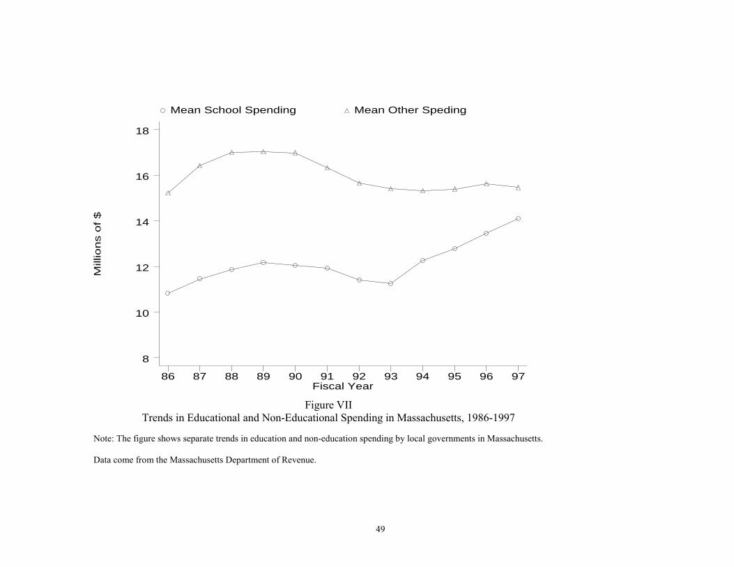
49

Mill

ions

of $

Fiscal Year

Mean School Spending Mean Other Speding

86 87 88 89 90 91 92 93 94 95 96 97

8

10

12

14

16

18

Figure VII

Trends in Educational and Non-Educational Spending in Massachusetts, 1986-1997 Note: The figure shows separate trends in education and non-education spending by local governments in Massachusetts.

Data come from the Massachusetts Department of Revenue.

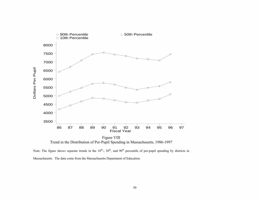
50

Do

llars

Pe

r P

up

il

Fiscal Year

90th Percentile 50th Percentile 10th Percentile

86 87 88 89 90 91 92 93 94 95 96 97

3500

4000

4500

5000

5500

6000

6500

7000

7500

8000

Figure VIII

Trend in the Distribution of Per-Pupil Spending in Massachusetts, 1986-1997 Note: The figure shows separate trends in the 10th-, 50th, and 90th percentile of per-pupil spending by districts in

Massachusetts. The data come from the Massachusetts Department of Education.

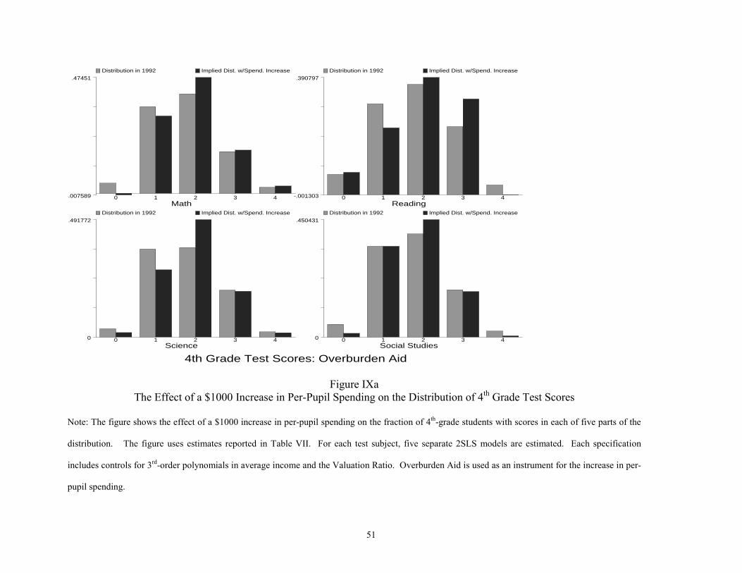
51

4th Grade Test Scores: Overburden Aid

Math-.007589

.47451 Distribution in 1992 Implied Dist. w/Spend. Increase

0 1 2 3 4Reading

-.001303


0 1 2 3 4

Science0


0 1 2 3 4Social Studies

0


0 1 2 3 4

Figure IXa

The Effect of a $1000 Increase in Per-Pupil Spending on the Distribution of 4th Grade Test Scores Note: The figure shows the effect of a $1000 increase in per-pupil spending on the fraction of 4th-grade students with scores in each of five parts of the

distribution. The figure uses estimates reported in Table VII. For each test subject, five separate 2SLS models are estimated. Each specification

includes controls for 3rd-order polynomials in average income and the Valuation Ratio. Overburden Aid is used as an instrument for the increase in per-

pupil spending.

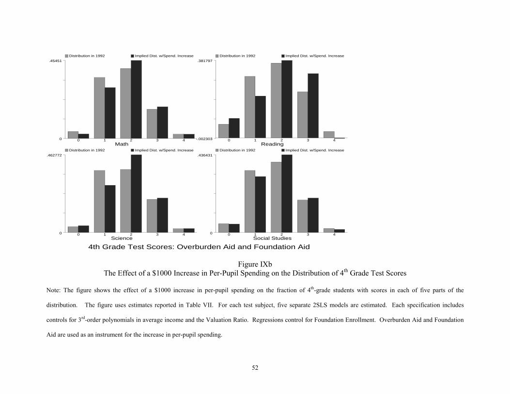
52

4th Grade Test Scores: Overburden Aid and Foundation Aid

Math0


0 1 2 3 4Reading

-.002303


0 1 2 3 4

Science0



0


0 1 2 3 4

Figure IXb

The Effect of a $1000 Increase in Per-Pupil Spending on the Distribution of 4th Grade Test Scores

Note: The figure shows the effect of a $1000 increase in per-pupil spending on the fraction of 4th-grade students with scores in each of five parts of the

distribution. The figure uses estimates reported in Table VII. For each test subject, five separate 2SLS models are estimated. Each specification includes

controls for 3rd-order polynomials in average income and the Valuation Ratio. Regressions control for Foundation Enrollment. Overburden Aid and Foundation

Aid are used as an instrument for the increase in per-pupil spending.

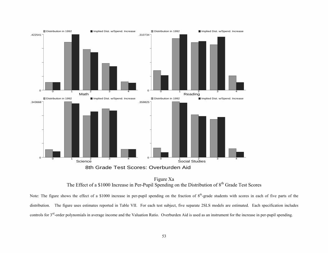
53

8th Grade Test Scores: Overburden Aid

Math0


0 1 2 3 4Reading

0


0 1 2 3 4

Science0



0


0 1 2 3 4

Figure Xa

The Effect of a $1000 Increase in Per-Pupil Spending on the Distribution of 8th Grade Test Scores Note: The figure shows the effect of a $1000 increase in per-pupil spending on the fraction of 8th-grade students with scores in each of five parts of the


controls for 3rd-order polynomials in average income and the Valuation Ratio. Overburden Aid is used as an instrument for the increase in per-pupil spending.

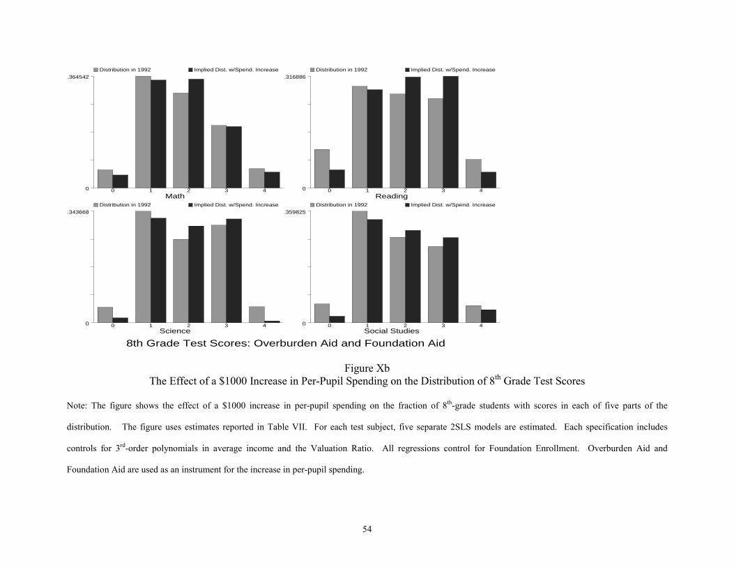
54

8th Grade Test Scores: Overburden Aid and Foundation Aid

Math0


0 1 2 3 4Reading

0


0 1 2 3 4

Science0



0


0 1 2 3 4

Figure Xb

The Effect of a $1000 Increase in Per-Pupil Spending on the Distribution of 8th Grade Test Scores

Note: The figure shows the effect of a $1000 increase in per-pupil spending on the fraction of 8th-grade students with scores in each of five parts of the


controls for 3rd-order polynomials in average income and the Valuation Ratio. All regressions control for Foundation Enrollment. Overburden Aid and

Foundation Aid are used as an instrument for the increase in per-pupil spending.

does money matter - the national bureau of economic … · · 2001-05-01discontinuities and...

Documents