
JANUARY 2016Capital Market Assumptions

VERUSINVESTMENTS.COM
SEATTLE 206‐622‐3700LOS ANGELES 310‐297‐1777
SAN FRANCISCO 415‐362‐3484
Table of contents
2
Summary 3
Inflation 8
Fixed income 10
Equities 16
Alternatives 20
Appendix 27

Summary
January 2016Capital Market Assumptions 3

MethodologyAPPROPRIATE FRAME OF REFERENCE— Over the short‐term, capital markets may reflect irrational investor behavior as prices diverge from fair value. — Mean reversion may occur over the long‐run as prices converge to underlying fundamentals due to long‐term investor rationality. — In our opinion, a 10‐year outlook is a reasonable time frame to expect fundamental valuation measures to mean‐revert.
January 2016Capital Market Assumptions 4
*We use local inflation for international developed equity and fixed income markets. When using local inflation rates, expected returns are adjusted for the implied currency effect based on currency forward contract rates (See Appendix)
Asset Return Methodology Volatility Methodology
Inflation 25% weight to the University of Michigan Survey 5‐10 year ahead inflation expectation and the Survey of Professional Forecasters(Fed Survey), and the remaining 50% to the market’s expectation for inflation as observed through the TIPS breakeven rate ‐
Cash Real yield estimate + inflation forecast Last 10 years of realized volatility
Bonds Nominal bonds: current annualized yieldReal bonds: real yield + inflation forecast Last 10 years of realized volatility
International Bonds* Current yield + implied currency effect Last 10 years of realized volatility
Credit Current option‐adjusted‐spread + U.S. 10‐year Treasury – default rate Last 10 years of realized volatility
International Credit* Current option‐adjusted‐spread + foreign 10‐year Treasury – default rate + implied currency effect Last 10 years of realized volatility
Private Credit High yield forecast + 2% illiquidity premium Last 10 years of realized volatility
Equity Dividends (current yield) + real earnings growth (historical average) + inflation on earnings (inflation forecast) + expected P/E change Last 10 years of realized volatility
International Developed Equity*
Dividends (current yield) + real earnings growth (historical average) + inflation on earnings (international inflation forecast) + expected P/E change + implied currency effect Last 10 years of realized volatility
Private Equity Small‐cap domestic equity forecast + 3% illiquidity premium 1.2 * last 10 years of realized U.S. small‐cap volatility
Commodities Cash + inflation forecast Last 10 years of realized volatility
Hedge Funds Return coming from traditional betas + 3% (alternative beta and alpha) 1.65 * last 10 years of realized volatility
Hedge Funds (FoF) Return coming from traditional betas + 3% (alternative beta and alpha) – 1% expected fund of funds management fee 1.65 * last 10 years of realized volatility
Core Real Estate Cap rate – capex + Inflation forecast 50% of REIT volatility
REITs Core real estate Last 10 years of realized volatility
Value‐Add Real Estate Core real estate + 2% Volatility to produce Sharpe Ratio (g) equal to core real estate
Opportunistic Real Estate Core real estate + 4% Volatility to produce Sharpe Ratio (g) equal to core real estate
Risk Parity Expected Sharpe Ratio * target volatility + cash rate Target volatility

10 year return & risk assumptions
Investors wishing to produce expected geometric return forecasts for their portfolios should use the arithmetic return forecasts provided here as inputs into that calculation, rather than the single‐asset‐class geometric return forecasts. This is the industry standard approach, but requires a complex explanation only a heavy quant could love, so we have chosen not to provide further details in this document – we will happily provide those details to any readers of this who are interested.
*Historical volatility of inflation. This is not a forecast.
5January 2016Capital Market Assumptions
Asset Class Index ProxyTen Year Return Forecast Standard Deviation
ForecastSharpe Ratio (g)
ForecastSharpe Ratio (a)
ForecastTen Year Historical Sharpe Ratio (g)
Ten Year Historical Sharpe Ratio (a)Geometric Arithmetic
EquitiesUS Large S&P 500 5.9% 7.0% 15.1% 0.26 0.33 0.40 0.46US Small Russell 2000 5.2% 7.0% 19.8% 0.16 0.25 0.28 0.37International Developed MSCI EAFE 9.2% 10.8% 18.5% 0.39 0.47 0.10 0.19International Small MSCI EAFE Small Cap 8.6% 10.4% 19.7% 0.33 0.43 0.17 0.26Emerging Markets MSCI EM 11.3% 13.6% 23.6% 0.39 0.49 0.10 0.22Global Equity MSCI ACWI 7.7% 9.1% 16.9% 0.34 0.42 0.21 0.29Private Equity Cambridge Private Equity 8.2% 11.0% 23.7% 0.26 0.37 1.01 1.08Fixed IncomeCash 30 Day T‐Bills 2.0% 2.0% 0.6% ‐ ‐ ‐US TIPS Barclays US TIPS 5 ‐ 10 2.7% 2.9% 6.3% 0.11 0.14 0.43 0.45US Treasury Barclays Treasury 7 ‐ 10 year 2.3% 2.5% 6.5% 0.04 0.07 0.67 0.68Global Sovereign ex US Barclays Global Treasury ex US 2.6% 2.9% 7.8% 0.07 0.11 0.24 0.28Core Fixed Income Barclays US Aggregate Bond 3.2% 3.3% 3.2% 0.37 0.40 1.02 1.00Core Plus Fixed Income Barclays US Corporate IG 4.2% 4.4% 6.0% 0.33 0.40 0.68 0.68Short‐Term Gov’t/Credit Barclays US Gov’t/Credit 1 ‐ 3 year 2.5% 2.5% 1.3% 0.37 0.37 1.20 1.30Short‐Term Credit Barclays Credit 1 ‐ 3 year 2.9% 3.0% 2.2% 0.40 0.45 1.01 0.98Long‐Term Credit Barclays Long US Corporate 4.2% 4.7% 10.5% 0.20 0.26 0.47 0.50High Yield Corp. Credit Barclays High Yield 7.1% 7.6% 10.6% 0.48 0.53 0.54 0.57Bank Loans S&P/LSTA 4.1% 4.5% 8.1% 0.24 0.31 0.38 0.40Global Credit Barclays Global Credit 2.4% 2.7% 6.9% 0.06 0.10 0.50 0.52Emerging Markets Debt (Hard) JPM EMBI Global Diversified 6.4% 6.8% 8.8% 0.50 0.54 0.64 0.65Emerging Markets Debt (Local) JPM GBI EM Global Diversified 6.8% 7.6% 12.9% 0.37 0.43 0.24 0.30Private Credit High Yield + 200 bps 9.1% 9.7% 10.9% 0.65 0.71 ‐ ‐OtherCommodities Bloomberg Commodity 4.0% 5.6% 18.2% 0.11 0.20 ‐0.42 ‐0.34Hedge Funds HFRI Fund of Funds 6.0% 6.4% 9.0% 0.44 0.49 0.19 0.21Hedge Funds (Fund of Funds) HFRI Fund of Funds 5.0% 5.4% 9.0% 0.33 0.38 ‐ ‐Core Real Estate NCREIF Property 4.7% 5.8% 13.2% 0.20 0.27 0.92 0.98Value‐Add Real Estate NCREIF Property + 200bps 6.7% 9.1% 23.3% 0.20 0.30 ‐ ‐Opportunistic Real Estate NCREIF Property + 400bps 8.7% 13.3% 33.2% 0.20 0.34 ‐ ‐REITs Wilshire REIT 4.7% 7.8% 26.4% 0.10 0.22 0.23 0.36Risk Parity 7.0% 7.5% 10.0% 0.50 0.54 ‐ ‐Inflation 2.0% ‐ 1.5%* ‐ ‐ ‐ ‐

‐15%
‐10%
‐5%
0%
5%
10%
15%
20%
25%
30%
Return
5th to 25th 25th to 50th 50th to 75th 75th to 95th 10 Year Forecast (Geometric)High Volatility Low Volatility
Range of likely 10 year outcomes
6January 2016Capital Market Assumptions
10 YEAR RETURN 90% CONFIDENCE INTERVAL

Relevant market movements— U.S. equity investors experienced mediocre returns during 2015 with the S&P 500 returning 1.4% and Russell 2000 producing a loss of 4.4%. A
stronger U.S. dollar proved a headwind for domestic equities, commodities, and unhedged exposure to foreign currency. Uncertainty surrounding the Fed’s rate hike triggered risk‐off sentiment. Higher valuations suggest that multiple expansion may be a headwind for some asset classes in the near future.
— International developed (EAFE) equity investors saw moderate gains on an unhedged basis with an annual loss of ‐0.8%. Investors with currency hedging programs were rewarded as the hedged index provided a return of 5%. European companies saw improved earnings growth over the year as balance sheets were less susceptible to heavy financial engineering. However, weak external demand may continue to dampen profit expectations. Additionally, further QE was launched this year by the ECB, providing a tailwind for equities.
— Emerging market equity markets experienced significant losses in 2015, with unhedged exposure to the index (MSCI EM) producing a return of ‐14.9%. Again, investors were rewarded for currency hedging which reduced losses on the year to ‐8.2%. Emerging market equities appear to be the most undervalued of the equity asset classes, though low valuations in many of these markets may be justified. Mean reversion would lead to healthy gains all else being equal and we forecast an additional 2% annual return to this asset class due to relatively cheap valuations.
— 2015 was characterized by several central bank rate cuts and implementation of easy monetary policy. These combined effects put significant downward pressure on yields globally. Global central bank policy continued to diverge, with the Bank of Japan and the European Central Bank implementing bond purchasing programs while the Fed implemented its first rate hike since 2006.
— U.S. breakeven inflation fell further over the year to 1.5% which reflects continued lower inflation expectations. With weak global growth and a stronger dollar, lack of inflation has become a global concern.
— Further divergence in monetary policy led to a strengthening of the U.S. dollar relative to developed market currencies and a decrease in U.S. long‐term interest rates.
— The last year was tough for risk parity strategies. Nearly all funds lost money due to flat or poor performance across most types of risk exposures.
— After a dramatic price drop off in 2014, investors experienced further declines with WTI oil closing 2015 at $37/barrel. Due to lower inflation expectations, expected future nominal returns remain moderate.
January 2016Capital Market Assumptions 7

Inflation
January 2016Capital Market Assumptions 8

INFLATION EXPECTATIONSUS 10YR ROLLING AVERAGE INFLATION SINCE 1923 FORECAST
InflationThe market’s expectations for 10‐year inflation can be inferred by taking the difference between the U.S. 10‐year Treasury yield and the U.S. 10‐year Treasury Inflation‐Protected (TIPS) yield (referred to as the breakeven inflation rate). While the breakeven rose in 2012, it fell throughout 2013 and then fell further in 2014 H2. The first half of 2015 saw moderate upward pressure in breakeven rates while the second half of 2015 was characterized by downwards movement with the latest breakeven pricing in a 1.5% rate of inflation over the next decade.
The latest University of Michigan Survey 5‐10 year forward inflation expectation, a survey of about 500 households around the nation, is 2.7%, slightly weaker than a year ago. Historically, this survey of inflation tends to be higher than actual future inflation.
A more stable indicator over time has been the Survey of Professional Forecasters (conducted quarterly). The most recent expectation for long‐term inflation is 2.15%.
January 2016Capital Market Assumptions 9
1.0
2.0
3.0
4.0
Dec‐11 Sep‐12 Jul‐13 Apr‐14 Jan‐15 Oct‐15US Ten Year Breakeven Inflation Rate
University of Michigan Survey 5‐10 Inflation Expectation
Survey of Profesional Forecasters
020406080100120140160180
‐3.5% ‐1.5% 0.5% 2.5% 4.5% 6.5% 8.5%
Coun
t of Inflatio
n Bu
cket Average:
3.15%Forecast: 1.98%
Source: U. of Michigan, Philly Fed, as of 12/31/15 Source: Bloomberg, as of 12/31/15 Source: Verus
10‐Year Forecast
University of Michigan Survey (25% weight) 2.70%
Survey of Professional Forecasters (25% weight) 2.15%
US 10‐Year TIPS Breakeven Rate (50% weight) 1.54%
Inflation Forecast 1.98%

Fixed income
January 2016Capital Market Assumptions 10

AVERAGE REAL RETURN US TREASURY ACTIVES CURVE FORECAST
CashThe yield curve shifted upward in 2015. While cash rates remained suppressed, the 3 month yield rose in December following the Fed rate hike.
Over rolling ten year time periods, the average historical real return to cash has been 14% of the real return to long bonds.
By applying this historical real return relationship, we arrive at a 4 bps expected real return to cash (14% of our 29 bps long bond real return forecast).
Adding our inflation forecast of 1.98% results in a nominal return to cash of 2.02%.
January 2016Capital Market Assumptions 11
0.0
0.5
1.0
1.5
2.0
2.5
Cash Long Bond
Percen
t (%)
14% of Long Bond
10‐Year Forecast
Cash 2.02%
Inflation Forecast ‐1.98%
Real Return 0.04%
‐0.50.00.51.01.52.02.53.03.5
0 10 20 30
Yield (percent %)
Years
12/31/2015 6/30/2015 12/31/2014
Source: Bloomberg Source: Bloomberg, as of 12/31/15 Source: Verus
US 10 YR TREASURY RATEMARKET ESTIMATE OF 10 YEAR RATE 1 YEAR OUT FORECAST
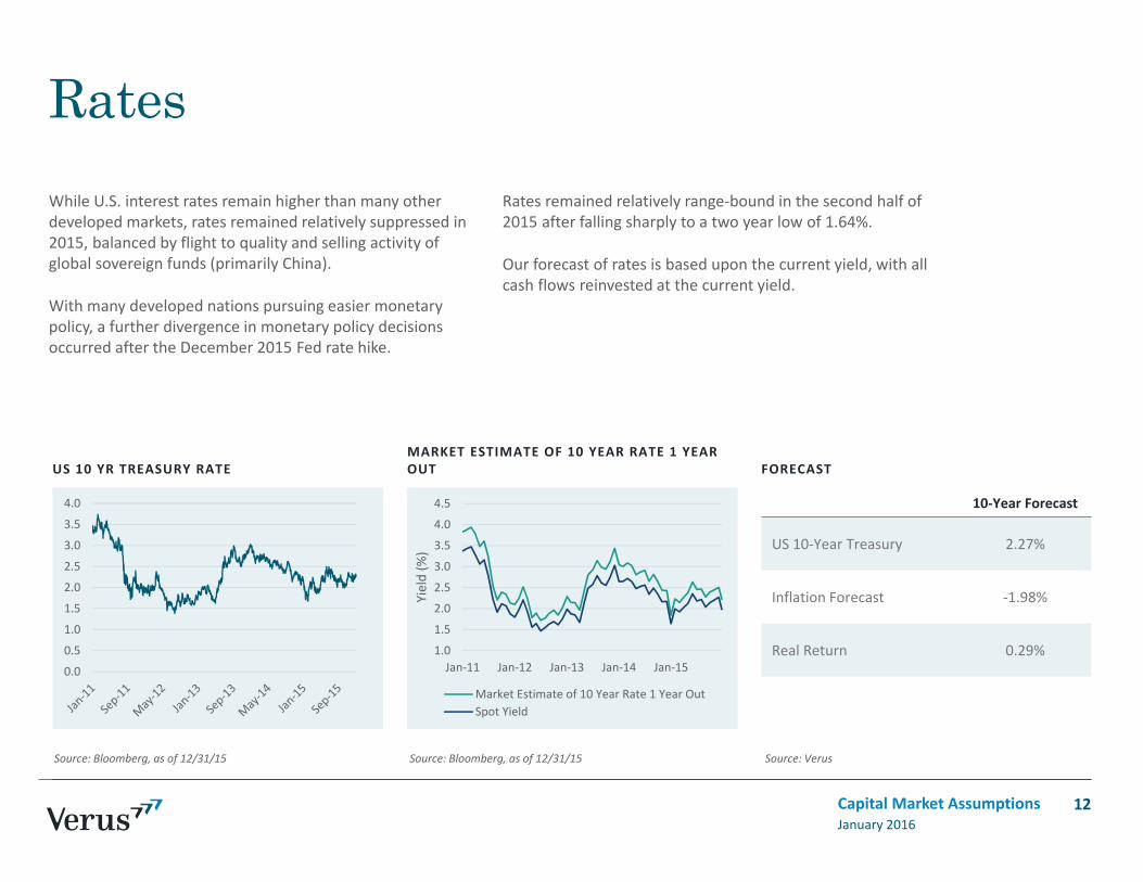
RatesWhile U.S. interest rates remain higher than many other developed markets, rates remained relatively suppressed in 2015, balanced by flight to quality and selling activity of global sovereign funds (primarily China).
With many developed nations pursuing easier monetary policy, a further divergence in monetary policy decisions occurred after the December 2015 Fed rate hike.
Rates remained relatively range‐bound in the second half of 2015 after falling sharply to a two year low of 1.64%.
Our forecast of rates is based upon the current yield, with all cash flows reinvested at the current yield.
January 2016Capital Market Assumptions 12
0.0
0.5
1.0
1.5
2.0
2.5
3.0
3.5
4.0 10‐Year Forecast
US 10‐Year Treasury 2.27%
Inflation Forecast ‐1.98%
Real Return 0.29%1.0
1.5
2.0
2.5
3.0
3.5
4.0
4.5
Jan‐11 Jan‐12 Jan‐13 Jan‐14 Jan‐15
Yield (%
)
Market Estimate of 10 Year Rate 1 Year OutSpot Yield
Source: Bloomberg, as of 12/31/15 Source: Bloomberg, as of 12/31/15 Source: Verus

NOMINAL YIELD VS REAL INFLATION EXPECTATIONS FORECAST
Real ratesWhile performance of TIPS can be volatile in the short‐term given sensitivity to interest rates, changes to inflation expectations, and demand for inflation protection, long‐term performance has tied closely to the Consumer Price Index.
To arrive at a nominal 10‐year forecast, we add the current real TIPS yield to our 10‐year inflation forecast.
January 2016Capital Market Assumptions 13
10‐Year Forecast
US 10‐Year TIPS Yield 0.70%
Inflation Forecast +1.98%
Nominal Return 2.68%
‐2.0%
‐1.0%
0.0%
1.0%
2.0%
3.0%
4.0%
Jan‐12 Jan‐13 Jan‐14 Jan‐15
U.S. R
eal Yield
US Nominal Yield US Real Yield Nominal ‐ Real
‐2
0
2
4
6
2001 2003 2005 2007 2009 2011 2013 2015
Inflatio
n (%
)
USA CPIUS Breakeven 10 YearUMich Expected Change in Price
Source: Bloomberg, as of 12/31/15 Source: Bloomberg, as of 12/31/15 Source: Verus

US CORE CREDIT SPREAD ROLLING EXCESS RETURN (10YR) FORECAST
Core fixedCredit fixed income return is composed of a bond term premium (duration) and credit spread.
We use appropriate default rates and credit spreads for each fixed income category to provide our 10 year return forecast.
Heavy anticipation of a Fed rate hike pushed yields higher for the first half of 2015. With heightened market volatility throughout the summer months, bonds rallied more as risk assets underperformed.
Within the core universe, investment grade credit spreads widened as companies took advantage of historically low interest rates to issue debt, making 2015 the largest year of issuance on record.
High M&A activity, increasing leverage, and less restrictive covenants may indicate we are later in the credit cycle. Effects of low energy prices increased the riskiness of both high grade and high yield debt instruments.
January 2016Capital Market Assumptions 14
0
1
2
3
4
Spread
(%)
US Core Spread Average US Core Spread
10‐Year Forecast
Barclays US Option‐Adjusted Spread +1.05%
Effective Default 0.10%
US 10‐Year Treasury +2.27%
Nominal Return 3.21%
Inflation Forecast ‐1.98%
Real Return 1.24%
‐0.4
0.0
0.4
0.8
1.2
1.6
Percen
t (%)
Barclays US Agg Bond ‐ BC Intermediate Treasury
Average excess return
Source: Barclays, as of 12/31/15 Source: Barclays, as of 12/31/15 Source: Verus

Credit summary
15January 2016Capital Market Assumptions
*We use local inflation for international developed equity and fixed income markets. When using local inflation rates, expected returns are adjusted for the implied currency effect based on currency forward contract rates (See Appendix)
CoreLong‐Term Credit Global Credit High Yield Bank Loans EM Debt (USD)
EM Debt (Local) Private Credit
Index BC US Aggregate BC Long US Corporate BC Global Credit BC US High Yield S&P LSTA JPM EMBI JPM GBI BC US High Yield +
2%
Method OAS + US10‐Year
OAS + US10‐Year
OAS + Global10‐Year Treasuries
OAS + US10‐Year LIBOR + Spread OAS + US
10‐Year Current YieldHigh Yield + 2%
illiquidity premium
Spread to Intermediate US Treasury
Long‐Term US Treasury
Global Long‐Term Treasuries
Intermediate US Treasury LIBOR Intermediate US
Treasury ‐ ‐
Default Assumption ‐0.5% ‐4.5% ‐3.0% ‐3.8% ‐3.5% ‐0.5% ‐0.5% ‐
Recovery Assumption 80% 95% 40% 40% 90% 60% 40% ‐
Spread 1.1% 2.1% 1.9% 7.1% 3.9% 4.4% ‐ ‐
Yield ‐ ‐ ‐ ‐ ‐ ‐ 7.1% ‐
Risk Free Yield 2.3% 2.3% 1.9% 2.3% 0.6% 2.3% ‐ ‐
Effective Default ‐0.1% ‐0.2% ‐1.8% ‐2.3% ‐0.4% ‐0.2% ‐0.3% ‐
Expected Currency Effect ‐ ‐ 0.4% ‐ ‐ ‐ ‐ ‐
Nominal Return 3.2% 4.2% 2.4% 7.1% 4.1% 6.4% 6.8% 9.1%
Inflation Forecast 2.0% 2.0% 2.0% 2.0% 2.0% 2.0% 2.0% 2.0%
Real Return 1.2% 2.2% 0.4% 5.1% 2.1% 4.4% 4.8% 7.1%

Equities
January 2016Capital Market Assumptions 16
TRAILING 10YR S&P 500 RETURN COMPOSITION SHILLER P/E SHILLER P/E ASSUMPTION
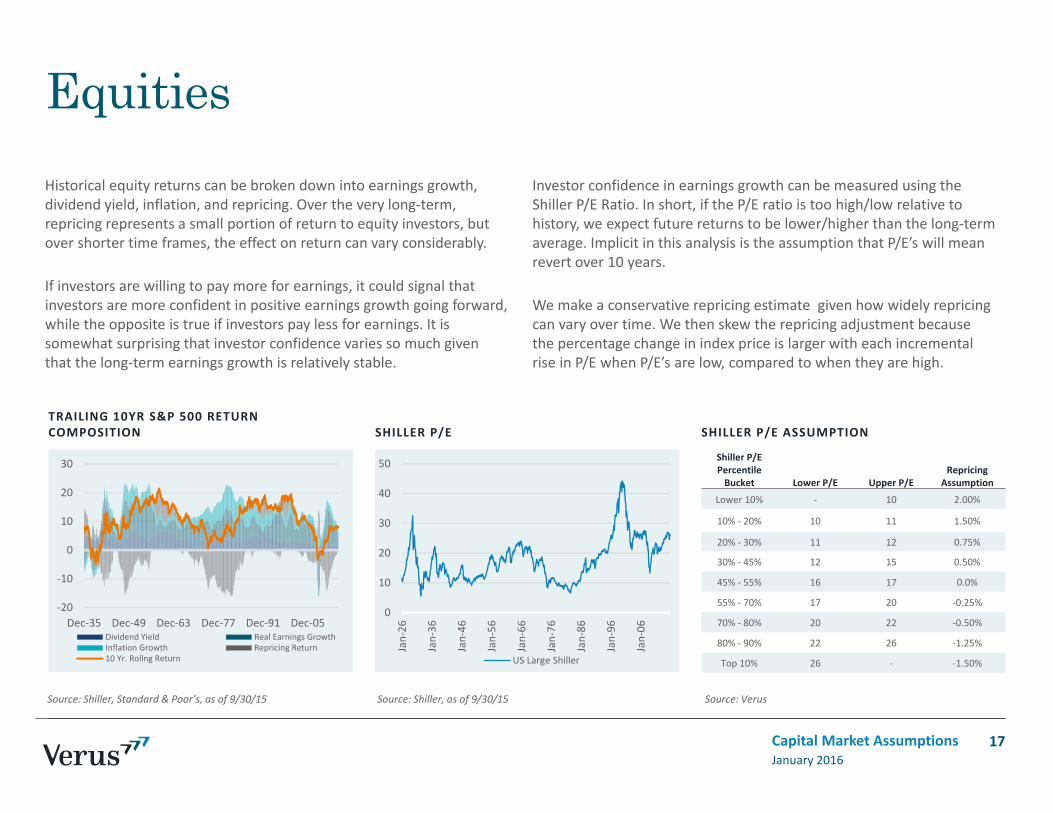
EquitiesHistorical equity returns can be broken down into earnings growth, dividend yield, inflation, and repricing. Over the very long‐term, repricing represents a small portion of return to equity investors, but over shorter time frames, the effect on return can vary considerably.
If investors are willing to pay more for earnings, it could signal that investors are more confident in positive earnings growth going forward, while the opposite is true if investors pay less for earnings. It is somewhat surprising that investor confidence varies so much given that the long‐term earnings growth is relatively stable.
Investor confidence in earnings growth can be measured using the Shiller P/E Ratio. In short, if the P/E ratio is too high/low relative to history, we expect future returns to be lower/higher than the long‐term average. Implicit in this analysis is the assumption that P/E’s will mean revert over 10 years.
We make a conservative repricing estimate given how widely repricing can vary over time. We then skew the repricing adjustment because the percentage change in index price is larger with each incremental rise in P/E when P/E’s are low, compared to when they are high.
January 2016Capital Market Assumptions
Source: Shiller, Standard & Poor’s, as of 9/30/15 Source: Shiller, as of 9/30/15 Source: Verus
17
Shiller P/EPercentile Bucket Lower P/E Upper P/E
Repricing Assumption
Lower 10% ‐ 10 2.00%
10% ‐ 20% 10 11 1.50%
20% ‐ 30% 11 12 0.75%
30% ‐ 45% 12 15 0.50%
45% ‐ 55% 16 17 0.0%
55% ‐ 70% 17 20 ‐0.25%
70% ‐ 80% 20 22 ‐0.50%
80% ‐ 90% 22 26 ‐1.25%
Top 10% 26 ‐ ‐1.50%
0
10
20
30
40
50
Jan‐26
Jan‐36
Jan‐46
Jan‐56
Jan‐66
Jan‐76
Jan‐86
Jan‐96
Jan‐06
US Large Shiller
‐20
‐10
0
10
20
30
Dec‐35 Dec‐49 Dec‐63 Dec‐77 Dec‐91 Dec‐05Dividend Yield Real Earnings GrowthInflation Growth Repricing Return10 Yr. Rollng Return

GLOBAL EQUITY P/E RATIO HISTORY MARKET PERFORMANCE (3YR ROLLING) FORECAST
Global equityGlobal Equity is a combination of U.S. large, international developed, Canada, and emerging market equities. We can therefore combine our existing return forecasts for each of these asset classes, along with a Canada equity forecast, to arrive at our global equity return forecast.
We use the MSCI ACWI Index as our benchmark for global equity and apply the country weights of this index to determine the weightings for our global equity return calculation. As with other equity asset classes, we use the
historical standard deviation of the benchmark (MSCI ACWI Index) for our volatility forecast.
The valuation of global equities are driven by the richness/cheapness of the underlying markets, as indicated by the current price/earnings ratio.
The underperformance of emerging markets in recent years has detracted from global equity returns, while U.S. equities have buoyed returns.
January 2016Capital Market Assumptions
Source: MSCI, as of 9/30/15 Source: MSCI, Standard & Poor’s, as of 12/31/15 Source: Verus
18
0510152025303540
Mar‐95 Mar‐00 Mar‐05 Mar‐10 Mar‐15
Current PE Average PE
Richer
CheaperAverage = 20.1
‐40
‐20
0
20
40
60
Dec‐01 Dec‐04 Dec‐07 Dec‐10 Dec‐13MSCI ACWI NR MSCI EAFE NRS&P 500 MSCI EM NR
Market Weight CMA return Weighted return
US Large 52.8% 5.89% 3.11%
Developed Large 34.5% 9.21% 3.18%
Emerging Markets 9.7% 11.25% 1.09%
Canada 3.0% 9.07% 0.27%
Global equity forecast 7.65%

Equity summary
19January 2016Capital Market Assumptions
*We use local inflation for international developed equity and fixed income markets. When using local inflation rates, expected returns are adjusted for the implied currency effect based on currency forward contract rates (See Appendix)**Average trailing P/E from previous 12 months is used
US Large US Small EAFE EAFE Small EM
Index S&P 500 Russell 2000 MSCI EAFE Large MSCI EAFE Small MSCI EM
Method Building Block Approach: current dividend yield + historical average real earnings growth + inflation on earnings + repricing + expected currency effect
Current Shiller P/E Ratio 24.4 36.8 14.2 ‐ 8.1
Regular P/E Ratio 18.3 33.5 19.0 23.5** 12.2
2015 Shiller P/E Expansion ‐7.2% ‐7.1% ‐2.7% ‐ ‐24.4%
2015 Regular P/E Expansion 0.5% 1.5% 15.9% 31.1% ‐3.9%
Current Shiller P/E Percentile Rank 84% 88% 13% ‐ 1%
Current Regular P/E Percentile Rank 69% 91% 56% 42%** 26%
Average of P/E Methods’ Percentile Rank 77% 90% 35% 42%** 8%
2015 Total Return 1.4% ‐4.4% ‐0.8% 9.6% ‐14.9%
Shiller PE History 1926 1988 1982 Not Enough History 2005
Long‐Term Average Shiller P/E 19.6 29.1 23.3 ‐ 16.9
Current Dividend Yield 2.2% 1.5% 3.3% 2.3% 2.9%
Long‐Term Average Real Earnings Growth 2.3% 3.0% 2.5% 2.9% 4.5%
Inflation on Earnings 2.0% 2.0% 1.4%* 1.4%* 2.0%
Repricing Effect (Estimate) ‐0.5% ‐1.3% 0.5% 0.5% 2.0%
Implied Currency Effect* ‐ ‐ 1.5%* 1.5%* ‐
Nominal Return 5.9% 5.2% 9.2% 8.6% 11.3%
Inflation Forecast 2.0% 2.0% 2.0% 2.0% 2.0%
Real Return 3.9% 3.2% 7.2% 6.6% 9.3%

Alternatives
January 2016Capital Market Assumptions 20
ROLLING 3YR PRIVATE EQUITY EXCESS RETURN (PE – U.S. SMALL CAP) PRIVATE EQUITY EXCESS RETURN FORECAST
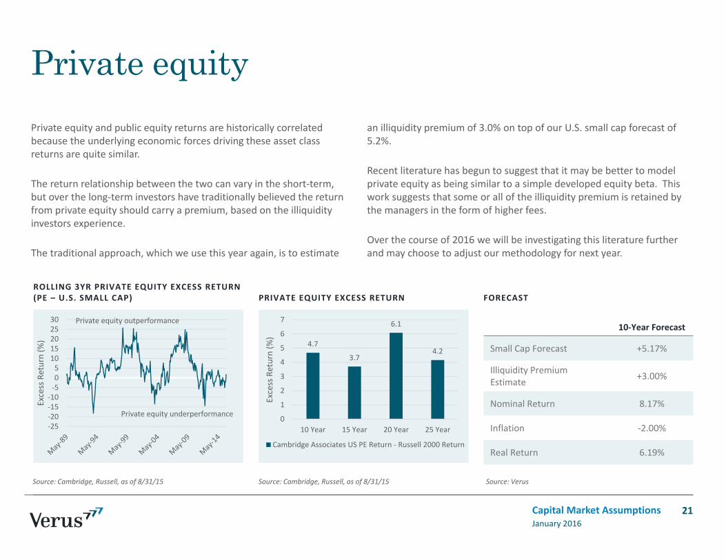
Private equityPrivate equity and public equity returns are historically correlated because the underlying economic forces driving these asset class returns are quite similar.
The return relationship between the two can vary in the short‐term, but over the long‐term investors have traditionally believed the return from private equity should carry a premium, based on the illiquidity investors experience.
The traditional approach, which we use this year again, is to estimate
an illiquidity premium of 3.0% on top of our U.S. small cap forecast of 5.2%.
Recent literature has begun to suggest that it may be better to model private equity as being similar to a simple developed equity beta. This work suggests that some or all of the illiquidity premium is retained by the managers in the form of higher fees.
Over the course of 2016 we will be investigating this literature further and may choose to adjust our methodology for next year.
January 2016Capital Market Assumptions
Source: Cambridge, Russell, as of 8/31/15 Source: Cambridge, Russell, as of 8/31/15 Source: Verus
21
10‐Year Forecast
Small Cap Forecast +5.17%
Illiquidity Premium Estimate +3.00%
Nominal Return 8.17%
Inflation ‐2.00%
Real Return 6.19%
‐25‐20‐15‐10‐5051015202530
Excess Return (%
)
Private equity outperformance
Private equity underperformance
4.7
3.7
6.1
4.2
0
1
2
3
4
5
6
7
10 Year 15 Year 20 Year 25 Year
Excess Return (%
)
Cambridge Associates US PE Return ‐ Russell 2000 Return

HISTORICAL BREAKDOWN OF BETAS
Hedge fundsTraditional betas explain approximately half of the variation in hedge fund net of fee returns, while the remaining unexplained portion can be attributed to alternative betas, skill, luck, or biases in the index.
We develop the systematic component of return by applying the historical weights of each traditional beta to our capital market assumptions.
As estimated by Ibbotson‐Chen‐Zhu 2010, the annualized unexplained portion of net of fee return is approximately 3.0%, which is statistically significant.
We add this estimate to our estimate of return coming from traditional betas to get a total net of fee return.
January 2016Capital Market Assumptions 22
Returns Explained by Systematic Factors
Equity market betas
Other traditional betas (bond, credit)
Alternative betas (value, carry, momentum, volatility)
Returns NOT Explained by Systematic Factors
Skill
Luck
Biases
TraditionalBetas Weight
2016 CMA (asset class average)
10‐Year Forecast
(weight*2016 CMA)
Equity 32% 6.62% 2.12%
Bonds ‐21% 4.59% ‐0.96%
Cash 89% 2.02% 1.8%
Traditional Beta Nominal Return 2.95%
Alternative Beta, Skill 3.00%
Nominal Return 5.95%
Inflation ‐1.98%
Real Return 3.97%
‐0.4‐0.20.00.20.40.60.81.01.21.4
Stocks Bonds Cash
Source: Ibbotson‐Chen‐Zhu 2010 Source: Ilmanen, Antti. Expected Returns Source: Verus
TRAILING 10YR NCREIF RETURN COMPOSITION PRIVATE REAL ESTATE REITS
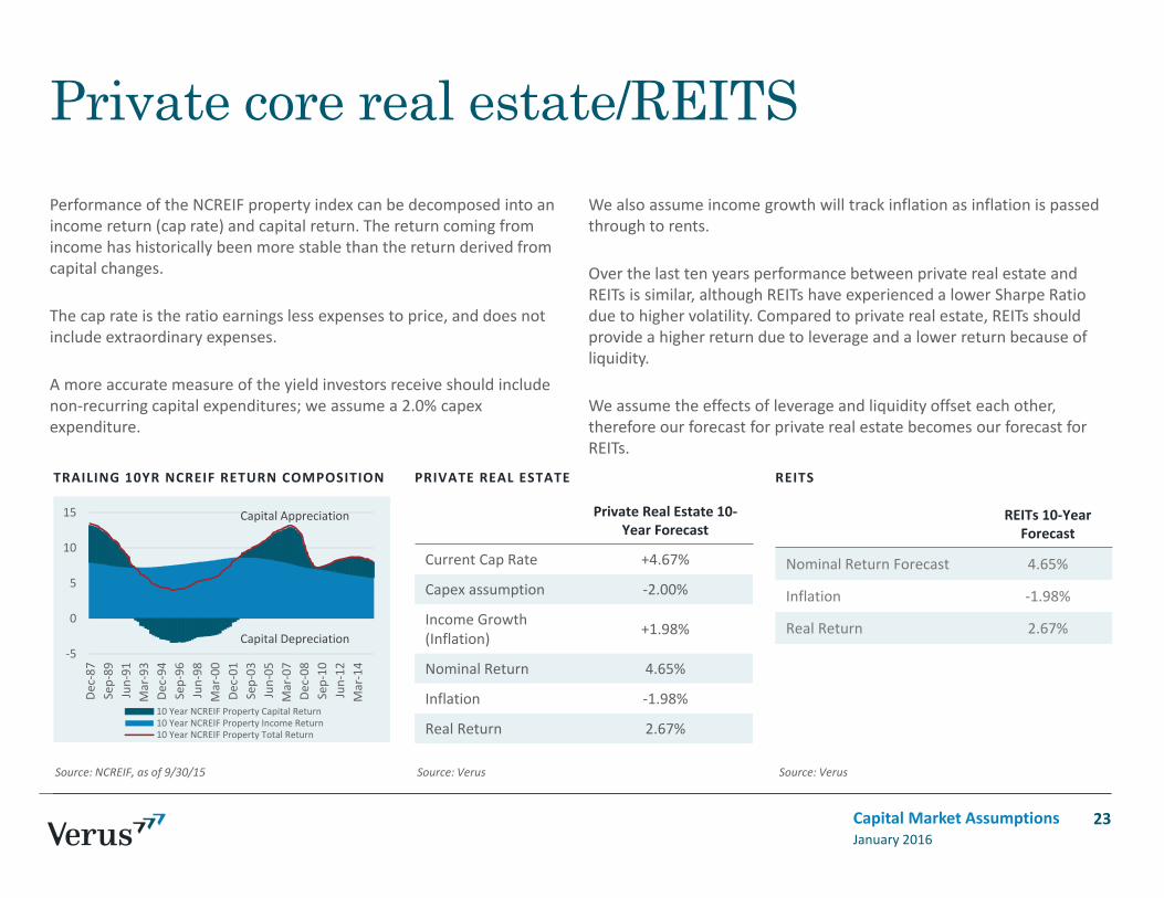
Private core real estate/REITSPerformance of the NCREIF property index can be decomposed into an income return (cap rate) and capital return. The return coming from income has historically been more stable than the return derived from capital changes.
The cap rate is the ratio earnings less expenses to price, and does not include extraordinary expenses.
A more accurate measure of the yield investors receive should include non‐recurring capital expenditures; we assume a 2.0% capex expenditure.
We also assume income growth will track inflation as inflation is passed through to rents.
Over the last ten years performance between private real estate and REITs is similar, although REITs have experienced a lower Sharpe Ratio due to higher volatility. Compared to private real estate, REITs should provide a higher return due to leverage and a lower return because of liquidity.
We assume the effects of leverage and liquidity offset each other, therefore our forecast for private real estate becomes our forecast for REITs.
January 2016Capital Market Assumptions
Source: NCREIF, as of 9/30/15 Source: Verus Source: Verus
23
Private Real Estate 10‐Year Forecast
Current Cap Rate +4.67%
Capex assumption ‐2.00%
Income Growth (Inflation) +1.98%
Nominal Return 4.65%
Inflation ‐1.98%
Real Return 2.67%
REITs 10‐Year Forecast
Nominal Return Forecast 4.65%
Inflation ‐1.98%
Real Return 2.67%‐5
0
5
10
15
Dec‐87
Sep‐89
Jun‐91
Mar‐93
Dec‐94
Sep‐96
Jun‐98
Mar‐00
Dec‐01
Sep‐03
Jun‐05
Mar‐07
Dec‐08
Sep‐10
Jun‐12
Mar‐14
10 Year NCREIF Property Capital Return10 Year NCREIF Property Income Return10 Year NCREIF Property Total Return
Capital Depreciation
Capital Appreciation

CAP RATE SPREADS
Value-add & opportunistic real estate
January 2016Capital Market Assumptions 24
Source: NCREIF, as of 9/30/15 Source: Verus
Value‐add real estate includes properties which are in need of renovation, repositioning, and/or lease‐up. Properties may also be classified as value‐add due to their lower quality and/or location. Opportunistic real estate can also include development and distressed or very complex transactions. Greater amounts of leverage are usually employed within these strategies. Leverage increases beta (risk) by expanding the purchasing power of property managers via a greater debt load, which magnifies gains or losses. Increased debt also results in greater interest rate sensitivity. An increase/decrease in interest rates may result in a write‐up/write‐down of fixed rate debt, since debt holdings are typically marked‐to‐market.
Performance of value‐add real estate is composed of the underlying private real estate market returns, plus a premium for additional associated risk, which is modeled here as 200 bps above our core real estate return forecast. Performance of opportunistic real estate strategies rest further out on the risk spectrum, and are modeled as 400 bps above the core real estate return forecast.
Additional expected returns above core real estate are justified by the higher inherent risk of properties which need improvement (operational or physical), price discounts built into properties located in non‐core markets, illiquidity, and the ability of real estate managers to potentially source attractive deals in this less‐than‐efficient marketplace.
Value‐Add 10‐Year Forecast
Opportunistic 10‐YearForecast
Premium above core +2.00% +4.00%
Current Cap Rate +4.67% +4.67%
Capex assumption ‐2.00% ‐2.00%
Income Growth (inflation) +1.98% +1.98%
Nominal Return 6.65% 8.65%
Inflation ‐1.98% ‐1.98%
Real Return 4.67% 6.67%
0112233445
0
2
4
6
8
10
1995
Q1
1995
Q4
1996
Q3
1997
Q2
1998
Q1
1998
Q4
1999
Q3
2000
Q2
2001
Q1
2001
Q4
2002
Q3
2003
Q2
2004
Q1
2004
Q4
2005
Q3
2006
Q2
2007
Q1
2007
Q4
2008
Q3
2009
Q2
2010
Q1
2010
Q4
2011
Q3
2012
Q2
2013
Q1
2013
Q4
2014
Q3
2015
Q2
Cap Rate Spread % (RHS) 10‐yreasury Yield % (LHS) Cap Rate % (LHS)

TRAILING 10YR BLOOMBERG COMMODITY RETURN COMPOSITION (%)
BLOOMBERG COMMODITY RETURN COMPOSITION (%) FORECAST
CommoditiesCommodity returns can be decomposed into four sources: collateral return (cash), inflation, spot changes, and roll yield.
Roll return represents either the backwardation or contangopresent in futures markets. Backwardation occurs when the futures price is below the spot price, which results in an additional profit. Contango occurs when the futures price is above the spot price, and this results in a loss to commodity investors. Historically, futures markets fluctuate between
backwardation and contango. Although roll return can be a large contribution to commodity returns, they are not considered in our forecast as there is no consistent methodology to forecast roll return. Over the most recent 10‐year period, roll return has been negative, contributing ‐10% to the Bloomberg Commodity total return.
Our 10‐year commodity forecast combines collateral (cash) return with inflation to arrive at the nominal return, and subtracts out inflation to arrive at the real return.
January 2016Capital Market Assumptions 25
10‐Year Forecast
Collateral Return (Cash) +2.02%
Roll Return +0.00%
Inflation +1.98%
Nominal Return 4.01%
Inflation ‐1.98%
Real Return 2.02%
‐20
‐10
0
10
20
30
Dec‐00 Dec‐04 Dec‐08 Dec‐12
Percen
t (%)
10 Year Roll Return 10 Year Cash Return10 Year US Inflation Growth 10 Year Spot Return10 Year Rolling Return
1.0
‐6.4
‐13.5
‐20
‐10
0
10
Last 20 Years Last 10 Years Last 5 Years
Return Com
position (%
)
Roll Yield Return Cash Return
US Inflation Growth Spot Return
Bloomberg Commodity Return
Source: MPI, Bloomberg, as of 12/31/15 Source: MPI, Bloomberg, as of 12/31/15 Source: Verus

VS TRADITIONAL ASSET CLASSES TRADITIONAL ASSET ALLOCATION RISK PARITY
Risk parityRisk parity is built upon the philosophy of allocating to risk premiarather than to asset classes. Because risk parity by definition aims to diversify risk, the actual asset allocation can appear very different from traditional asset class allocation.
We model risk parity using an assumed Sharpe Ratio of 0.5, which takes into consideration the historical performance of risk parity. The expected return of Risk Parity is determined by this Sharpe Ratio forecast, along with a 10% volatility assumption.
We used a 10‐year historical return stream from a market‐leading product to represent risk parity correlations relative to the behaviors of each asset class. Through greater diversification exposures, risk parity funds are suggested to be better able to withstand various difficult economic environments ‐ reducing volatility without sacrificing return, over longer periods.
It is difficult to model risk parity, since strategies can differ significantly across firms/strategies. Risk parity almost always requires explicit leverage. The amount of leverage will depend on the specific strategy implementation style, as well as expected correlations and volatility.
January 2016Capital Market Assumptions
Source: MPI, as of 12/31/15 Source: Verus Source: VerusNote: Risk parity is modeled here using the AQR GRP‐EL 10% Volatility fund. Performance is back tested prior to February 2015
26
Equity Risk
Interest Rate Risk
Credit Risk
Inflation Risk
Equity Risk
Interest Rate Risk
Credit Risk
Inflation Risk
‐20
0
20
40
Dec‐93 Dec‐98 Dec‐03 Dec‐08 Dec‐13
Return (%
)
S&P 500 TR USD Barclays US Agg Bond TR USD
Risk Parity 10% Vol Bloomberg Commodity TR USD

Appendix
January 2016Capital Market Assumptions 27
‐1.5%
‐1.0%
‐0.5%
0.0%
0.5%
1.0%
1.5%
2.0%
Expe
cted
Return
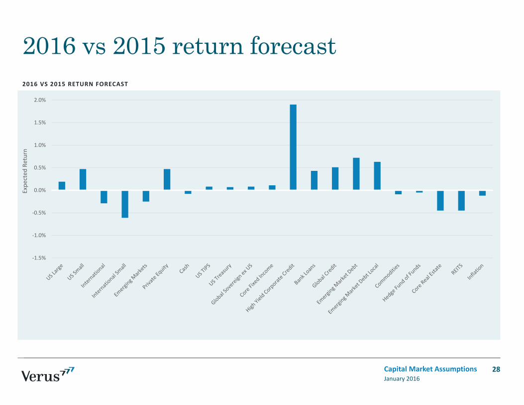
2016 vs 2015 return forecast
28January 2016Capital Market Assumptions
2016 VS 2015 RETURN FORECAST

The currency effect
— This last year has re‐emphasized the important effect that currency returns can have on unhedged international portfolios. Verus has traditionally taken the view that we do not attempt to forecast currency market movement.
— When forecasting currencies, the “no opinion” position is reflected in the currency forward markets. This market prices currencies at a range of forward dates based on interest rate differentials ‐ they represent the SPOT currency price for FORWARD delivery. Divergence from these rates is described as currency surprise.
— Investors with no active opinion regarding which direction exchange rates are headed would expect to earn the local currency return of foreign assets after correcting for the forward exchange rate (as priced by the currency forward market). We describethese returns as “hedged”.
— An investor with no active view regarding which direction exchange rates are headed would expect the unhedged and hedged returns from a foreign asset exposure to be identical.
— We therefore forecast foreign assets in local currency terms, then correct for expected currency movement based on currency forward market prices. We do this using 10‐year forward rates. Because Verus has not historically expressed a view on currency, this is directly comparable to our previous forecasts.
January 2016Capital Market Assumptions 29

Currency adjustment
THE EXPECTED CURRENCY EFFECT CAN BE CALCULATED BY IDENTIFYING THE FOLLOWING:
1. Today’s currency spot rate
2. The price of a forward currency contract with a maturity equal to our forecasting horizon (10 years)
3. The annualized currency effect implied by this currency contract
EQUATION:
[(10 year contract rate)/(spot rate)]^(1/years)‐1
FOR EXAMPLE:
If a US investor wishes to determine the likely currency affect of investing in Euro‐denominated investments, and the EURUSD is currently tradingat 1.13 (the spot rate), and a 10‐year EURUSD currency forward contract is trading at 1.30, then the investor can use the equation below tocalculate the implied currency effect:
(1.30/1.13)^(1/10) ‐ 1 = 1.41%
This tells us that the expected annualized currency effect for a US investor investing in Euro‐denominated assets is a +1.41% currency return.
January 2016Capital Market Assumptions 30

Correlation assumptions
Note: Correlation assumptions are based on the last ten years. Private Equity and Real Estate correlations are especially difficult to model – we have therefore used BarraOne correlation data to strengthen these correlation estimates.
31January 2016Capital Market Assumptions
Cash US Large US Small Developed
LargeDeveloped
Small EM Global Equity PE US TIPS US
Treasury
Global Sovereign exUS
US Core US Core Plus
Short –Term Govt/Credit
Short‐Term Credit
Long‐Term Credit US HY Bank
LoansGlobal Credit EMD USD EMD
LocalCommodi
tiesHedge Funds
Real Estate REITs Risk Parity Inflation
Cash 1US Large ‐0.1 1US Small ‐0.1 0.9 1Developed
Large ‐0.1 0.9 0.8 1
Developed Small ‐0.1 0.8 0.8 1.0 1
EM 0.0 0.8 0.7 0.9 0.9 1Global Equity ‐0.1 0.9 0.8 0.9 0.9 0.9 1
PE ‐0.2 0.7 0.7 0.8 0.8 0.7 0.7 1US TIPS 0.0 0.2 0.1 0.3 0.3 0.3 0.3 0.1 1
US Treasury 0.1 ‐0.3 ‐0.3 ‐0.2 ‐0.2 ‐0.2 ‐0.2 ‐0.2 0.6 1Global
Sovereign exUS 0.1 0.2 0.2 0.4 0.4 0.4 0.3 0.1 0.6 0.5 1
US Core 0.1 0.0 0.0 0.1 0.1 0.2 0.1 0.0 0.8 0.9 0.6 1US Core Plus ‐0.2 0.3 0.3 0.5 0.5 0.5 0.4 0.4 0.7 0.5 0.5 0.7 1Short –Term Govt/Credit 0.4 ‐0.1 ‐0.1 0.1 0.1 0.1 0.0 ‐0.2 0.6 0.6 0.6 0.7 0.4 1
Short‐Term Credit 0.1 0.3 0.2 0.4 0.4 0.4 0.3 ‐0.1 0.4 0.1 0.4 0.5 0.4 0.7 1
Long‐Term Credit ‐0.1 0.3 0.2 0.4 0.4 0.4 0.3 0.1 0.6 0.5 0.5 0.8 0.8 0.5 0.6 1
US HY ‐0.1 0.7 0.7 0.8 0.8 0.8 0.8 0.6 0.4 ‐0.2 0.3 0.2 0.6 0.1 0.5 0.5 1Bank Loans ‐0.1 0.6 0.5 0.5 0.6 0.5 0.5 0.2 0.2 ‐0.4 0.0 0.0 0.2 ‐0.1 0.6 0.3 0.8 1Global Credit 0.0 0.6 0.5 0.8 0.8 0.7 0.7 0.5 0.6 0.2 0.7 0.6 0.8 0.5 0.6 0.7 0.8 0.5 1EMD USD ‐0.1 0.6 0.5 0.7 0.7 0.7 0.7 0.6 0.7 0.2 0.5 0.6 0.8 0.3 0.5 0.7 0.8 0.5 0.9 1EMD Local 0.1 0.7 0.6 0.8 0.8 0.8 0.8 0.6 0.5 0.1 0.6 0.4 0.5 0.3 0.4 0.5 0.7 0.4 0.8 0.8 1
Commodities 0.1 0.5 0.4 0.6 0.6 0.6 0.6 0.2 0.3 ‐0.2 0.4 0.1 0.2 0.2 0.4 0.2 0.5 0.4 0.6 0.5 0.6 1Hedge Funds ‐0.1 0.7 0.6 0.8 0.8 0.8 0.8 0.6 0.2 ‐0.3 0.1 0.0 0.4 ‐0.1 0.3 0.2 0.6 0.5 0.6 0.5 0.5 0.6 1Real Estate ‐0.1 0.3 0.3 0.3 0.3 0.3 0.6 0.3 0.0 ‐0.1 0.1 0.0 0.1 ‐0.1 0.0 0.1 0.2 0.0 0.2 0.2 0.2 0.0 0.2 1
REITs ‐0.1 0.7 0.8 0.7 0.6 0.6 0.7 0.6 0.3 ‐0.1 0.3 0.3 0.4 0.0 0.2 0.4 0.7 0.5 0.6 0.6 0.6 0.3 0.4 0.4 1Risk Parity 0.1 0.5 0.4 0.5 0.5 0.5 0.5 0.0 0.6 0.3 0.6 0.6 0.4 0.5 0.7 0.6 0.5 0.4 0.7 0.6 0.6 0.6 0.4 ‐0.1 0.4 1Inflation 0.1 0.1 0.1 0.1 0.2 0.2 0.2 0.1 0.1 ‐0.3 0.0 ‐0.3 0.0 ‐0.2 ‐0.1 ‐0.3 0.2 0.3 0.1 0.1 0.1 0.3 0.3 0.0 0.1 0.0 1

Notices & disclosuresPast performance is no guarantee of future results. This report or presentation is provided for informational purposes only and is directed to institutional clients and eligible institutional counterparties only and should not be relied upon by retail investors. Nothing herein constitutes investment, legal, accounting or tax advice, or a recommendation to buy, sell or hold a security or pursue a particular investment vehicle or any trading strategy. The opinions and information expressed are current as of the date provided or cited only and are subject to change without notice. This information is obtained from sources deemed reliable, but there is no representation or warranty as to its accuracy, completeness or reliability. Verus Advisory Inc. and Verus Investors, LLC expressly disclaim any and all implied warranties or originality, accuracy, completeness, non‐infringement, merchantability and fitness for a particular purpose. This report or presentation cannot be used by the recipient for advertising or sales promotion purposes.
The material may include estimates, outlooks, projections and other “forward‐looking statements.” Such statements can be identified by the use of terminology such as “believes,” “expects,” “may,” “will,” “should,” “anticipates,” or the negative of any of the foregoing or comparable terminology, or by discussion of strategy, or assumptions such as economic conditions underlying other statements. No assurance can be given that future results described or implied by any forward looking information will be achieved. Actual events may differ significantly from those presented. Investing entails risks, including possible loss of principal. Risk controls and models do not promise any level of performance or guarantee against loss of principal.
“VERUS ADVISORY™ and VERUS INVESTORS™ and any associated designs are the respective trademarks of Verus Advisory, Inc. and Verus Investors, LLC. Additional information is available upon request.
January 2016Capital Market Assumptions 32


