
저 시-비 리- 경 지 2.0 한민
는 아래 조건 르는 경 에 한하여 게
l 저 물 복제, 포, 전송, 전시, 공연 송할 수 습니다.
다 과 같 조건 라야 합니다:
l 하는, 저 물 나 포 경 , 저 물에 적 된 허락조건 명확하게 나타내어야 합니다.
l 저 터 허가를 면 러한 조건들 적 되지 않습니다.
저 에 른 리는 내 에 하여 향 지 않습니다.
것 허락규약(Legal Code) 해하 쉽게 약한 것 니다.
Disclaimer
저 시. 하는 원저 를 시하여야 합니다.
비 리. 하는 저 물 리 목적 할 수 없습니다.
경 지. 하는 저 물 개 , 형 또는 가공할 수 없습니다.

공학박사학위논문
기계 시스템 건전성 평가를 위한 유효독립성
기반 센서 네트워크 디자인 연구
Effective Independence-Based Sensor Network Design for
Health Assessment of Engineered Systems
2017년 2월
서울대학교 대학원
기계항공공학부
김 태 진

i
Abstract
Effective Independence-Based Sensor
Network Design for Health Assessment of
Engineered Systems
Taejin Kim
Department of Mechanical and Aerospace Engineering
The Graduate School
Seoul National University
The failure of an engineered system not only results in an enormous property loss, but
also causes a substantial societal loss. The discipline of prognostics and health
management (PHM) recently has received great attention as a solution to prevent
unexpected failures of engineered systems. The goal of PHM is to detect anomaly states,
to predict potential failures of a system, and to plan an optimal management schedule.
PHM is composed of five essential functions: 1) sensing, 2) reasoning, 3) diagnostics, 4)
prognostics, and 5) management. The sensing function, in which sensory data is acquired
from the system of interest, is a core element needed for cost-effective execution of PHM.
The success of the remaining functions in PHM highly depends on the quality of the data
obtained by the sensing function.

ii
The research described herein describes the investigation of two original ideas of
optimal sensor placement (OSP) for the PHM sensing function. These ideas are aimed to
enable cost-effective and robust sensor data acquisition from the system. The first idea is
a stochastic effective independence (EFI) method, referred to as an energy-based stochastic
EFI method; the proposed method overcomes the drawbacks of existing OSP methods in
the sensing function. In Research Thrust 1, the stochastic sensor network design is
proposed. It takes the uncertainty of the system into consideration to give more accurate
representation of the system than the deterministic sensor network design in the mean sense.
Also, the explicit form of the proposed method has the benefit of lower computational
requirements, as compared to the sampling-based stochastic approach. In Research Thrust
2, a robust sensor network design that considers the latent failure of the sensor is introduced.
The proposed robust sensor network is designed to tolerate the partial failure of the sensor;
thus, it contributes to the safety of the sensor network. The proposed method is validated
to have accuracy that is comparable to the optimal sensor network design in normal
conditions, and higher accuracy for situations in which there is a partial failure of the given
sensor network.
Keywords: Sensor network design
Effective independence (EFI) method
EigenMap method
Stochastic effective independence method
Robust sensor network design
Student Number: 2011-20702

iii
Contents
Abstract ................................................................................................ i
Contents ............................................................................................. iii
List of Tables ....................................................................................... v
List of Figures .................................................................................... vi
Nomenclature ..................................................................................... ix
Chapter 1. Introduction ..................................................................... 1
1.1 Background and Motivation ............................................................................ 1
1.2 Research Objectives and Scopes ...................................................................... 3
1.3 Dissertation Overview ..................................................................................... 5
Chapter 2. Literature Review ........................................................... 7
2.1 Linear Independence of a System .................................................................... 7
2.2 Model-based Sensor Placement Method: Effective Independence Method .. 10
2.3 Energy-Based Sensor Placement Method ...................................................... 14
2.4 Data-Based Sensor Placement Method: EigenMap Method .......................... 15
Chapter 3. Stochastic Sensor Network Design .............................. 18
3.1 Stochastic Finite Element Method ................................................................. 18
3.1.1 Principle of Stochastic Perturbation .................................................... 18
3.1.2 Stochastic Eigenvalue Problem ........................................................... 19
3.2 Stochastic Effective Independence Method ................................................... 21

iv
3.3 Energy-Based Stochastic EFI Method ........................................................... 30
3.4 Case Study ..................................................................................................... 31
3.4.1 Truss Bridge Structure ........................................................................ 32
3.4.2 Sensor Placement Under Uncertainty ................................................. 34
3.4.2.1 Monte Carlo Simulation .............................................................. 34
3.4.2.2 SEFI Method................................................................................ 38
3.5 Conclusion ..................................................................................................... 53
Chapter 4. Robust Sensor Network Design ................................... 55
4.1 Battery System ............................................................................................... 55
4.1.1 Battery Pack Overview ....................................................................... 55
4.1.2 Heat Generation Model ....................................................................... 58
4.1.3 Model Calibration and Validation ....................................................... 62
4.2 Robust Sensor Network Design ..................................................................... 65
4.3 Case Study ..................................................................................................... 72
4.3.1 Case 1: Different Heat Generation for the Cells ................................. 72
4.3.2 Case 2: Forced Convection ................................................................. 76
4.4 Conclusion ..................................................................................................... 83
Chapter 5. Contributions and Future Work ................................. 86
5.1 Contributions and Impacts ............................................................................. 86
5.2 Suggestions for Future Research ................................................................... 88
References ......................................................................................... 90
Abstract (Korean) ............................................................................ 90

v
List of Tables
Table 1-1 Challenges, objectives, and benefits of this research ......................................... 6
Table 2-1 Pseudo-code for the effective independence method ....................................... 13
Table 3-1 The set of 10 sensors selected by EFI using the deterministic EFI, MCS, and
stochastic EFI ........................................................................................................... 40
Table 3-2 The average estimation error of MCS and SFEM for given cases ................... 45
Table 3-3 The set of 10 sensors selected by strain-energy-based EFI using the
deterministic EFI, MCS, and stochastic EFI ............................................................ 47
Table 3-4 The set of 10 sensors selected by kinetic-energy-based EFI using the
deterministic EFI, MCS, and stochastic EFI ............................................................ 50
Table 3-5 The simulation time of MCS with 1,000 simulations and stochastic EFI for a 2-
D truss bridge ........................................................................................................... 52
Table 4-1 The RMS error of OSP and ROSP methods for case 1 .................................... 75
Table 4-2 The RMS error of OSP and ROSP methods for case 2 .................................... 78
Table 4-3 Sensor placement corresponding to the number of sensors and estimation
accuracy ................................................................................................................... 80
Table 4-4 Sensor locations and the estimation accuracy for different mode shapes ........ 82

vi
List of Figures
Figure 2-1 Linear independence of the system according to the sensor locations: (a) If the
data is measurable in every DOF, the mode shapes are linearly independent, (b) if
the data is partially measurable, the mode shapes could be linearly dependent,
depending on the measured DOFs. ............................................................................ 9
Figure 2-2 Schematic performance comparison of EFI and the EigenMap method. ....... 17
Figure 3-1 Transformation of the row of the mode shape matrix (Φm) to the absolute
identification space. ................................................................................................. 24
Figure 3-2 Example of the transformation of the row of the mode shape matrix (Φm) to
the absolute identification space. The arrow indicates the deterministic
transformation and the point cluster indicates the probabilistic transformation
generated by the MCS method. ................................................................................ 29
Figure 3-3 Two-dimensional truss bridge. ....................................................................... 33
Figure 3-4 Target mode representation with mean and standard deviation: (a) 1st mode,
(b) 2nd mode, (c) 3rd mode, and (d) 4th mode. ....................................................... 33
Figure 3-5 Histograms of 1,000 EFI simulations with stochastic Young’s modulus with
the mean 70 GPa: (a) the standard deviation 0.05×70 GPa, (b) the standard deviation
0.1×70 GPa, and (c) 0.15×70 GPa. .......................................................................... 35
Figure 3-6 Histograms of 1,000 strain energy EFI simulations with stochastic Young’s
modulus with the mean 70 GPa: (a) the standard deviation 0.05×70 GPa, (b) the
standard deviation 0.1×70 GPa, and (c) 0.15×70 GPa. ............................................ 37

vii
Figure 3-7 Determinant of the Fisher information matrix by (a) EFI with standard
deviation of 0.05×70 GPa , (b) MCS with standard deviation of 0.05×70 GPa , (c)
stochastic EFI with standard deviation of 0.05×70 GPa , (d) EFI with standard
deviation of 0.1×70 GPa , (e) MCS with standard deviation of 0.1×70 GPa , (f)
stochastic EFI with standard deviation of 0.1×70 GPa , (g) EFI with standard
deviation of 0.15×70 GPa , (h) MCS with standard deviation of 0.15×70 GPa , and
(i) stochastic EFI with standard deviation of 0.15×70 GPa. .................................... 41
Figure 3-8 The target deflections of a truss bridge with the mean Young’s modulus ...... 44
Figure 3-9 The estimated deflection for a randomly generated truss bridge generated by:
(a) MCS for case 1, (b) MCS for case 2, (c) SFEM for case 1, and (d) SFEM for
case 2 ........................................................................................................................ 44
Figure 3-10 Determinant of the Fisher information matrix by (a) energy-based EFI with
standard deviation of 0.05×70 GPa , (b) MCS with standard deviation of 0.05×70
GPa , (c) stochastic EFI with standard deviation of 0.05×70 GPa , (d) energy-based
EFI with standard deviation of 0.1×70 GPa , (e) MCS with standard deviation of
0.1×70 GPa , (f) stochastic EFI with standard deviation of 0.1×70 GPa , (g) energy-
based EFI with standard deviation of 0.15×70 GPa , (h) MCS with standard
deviation of 0.15×70 GPa , and (i) stochastic EFI with standard deviation of
0.15×70 GPa. ........................................................................................................... 48
Figure 4-1 (a) Battery pack geometry, and (b) the lumped parameter model. ................. 57
Figure 4-2 (a) HPPC test profile, and (b) impedance values at SOC levels. ................... 60
Figure 4-3 (a) Entropic heat test profile and (b) dVocv/dT. ............................................... 61
Figure 4-4 The measured and simulated temperatures under 1C (=2.6A) discharge
current. ..................................................................................................................... 63

viii
Figure 4-5 UDDS test results: (a) UDDS current profile, and (b) the measured and the
simulated temperature. ............................................................................................. 64
Figure 4-6 The temperature distribution of a battery pack under constant current: (a)
temperature change across time, and (b) the temperature distribution at 83 min. ... 66
Figure 4-7 The first four eigenvectors of the training data set: (a) 1st mode, (b) 2nd
mode, (c) 3rd mode, and (d) 4th mode. .................................................................... 67
Figure 4-8 The sensor locations: (a) Optimal sensor placement (OSP), and (b) the robust
optimal sensor placement. ........................................................................................ 71
Figure 4-9 The temperature distribution of the battery pack under a constant current
realized from the random distribution: (a) temperature change across time, and (b)
the temperature distribution at 83 min. .................................................................... 74
Figure 4-10 The temperature distribution of a battery pack under forced convection: (a)
temperature change across time, and (b) the temperature distribution at 83 min. ... 77

ix
Nomenclature
DOF = Degree of Freedom
EFI = Effective Independence Method
FE model = Finite Element model
FIM = Fisher Information Matrix
OSP = Optimal Sensor Placement
PHM = Prognostics and Health Management
RMS = Root Mean Square
ROSP = Robust Optimal Sensor Placement
RUL = Remaining Useful Life
SFEM = Stochastic Finite Element Method
UDDS = Urban Dynamometer Driving Schedule
b = random variable
b0 = expectation of random variable b
C = covariance matrix
ED = effective independence distribution
FE = fractional eigenvalue matrix
f = state function
f0 = function value evaluated at expectation
K = stiffness matrix of the FE model
k = number of sensors

x
M = mass matrix of the FE model
M = number of data sets
n = dimension of the finite element model
p = probability density function
q = amplitude corresponding to basis vector of the FE model
�̂� = estimated amplitude corresponding to basis vector of the FE model
Q = redefined Fisher information matrix
Q0 = Fisher information matrix
QKE = kinetic energy
Qs = stochastic Fisher information matrix
QSE = strain energy
Q0s = Fisher information matrix evaluated at the expectation of the random variable
W = weight matrix
w = Gaussian white noise in the signal
y = arbitrary mechanical signal
ys = measured signal
�̂� = regenerated signal
ε = perturbation
λ = eigenvalue
μ = mean
σ = variance of signal noise
Φ = mode shape matrix

xi
ΦE = basis matrix from the covariance matrix
Φm = mean mode shape matrix
Φr = mode shape matrix with measured DOF
Φs = mode shape matrix with measured DOF and selected basis
Φv = residual mode shape matrix
ψ = eigenvectors of the Fisher information matrix

1
Chapter 1. Introduction
1.1 Background and Motivation
The failure of a system not only results in enormous damage to the system itself,
such as the downtime cost and the restoration cost, failure also causes societal costs,
including injury or even loss of human life. As a solution to prevent system failures,
recently the field of prognostics and health management (PHM) is getting wide
attention [1-5]. The purpose of the PHM is to avoid any kind of failure, and to plan
optimal management schedules by estimating the current status, and predicting the
remaining useful life (RUL) of a system.
The PHM is composed of four functions; specifically, the sensing, reasoning,
prognostics, and management functions. In the sensing function, sensors are placed
on the system to obtain the proper data that gives relevant information for the
reasoning function. In the following stage of reasoning, the obtained data is analyzed
to verify the current conditions of the system. Then, the prognostics function predicts
the RUL based on the past and current conditions that were verified during the
reasoning function. Finally, using all the information up to the prognostics function,
proper decisions about the operation and maintenance are made as part of the
management function.

2
As seen in the overall process of PHM, sensing is the beginning step of the whole
process. Each subsequent step depends on the sensing step. Therefore, proper
sensing is very important for successful PHM. If successful implementation of this
step is possible, the following diagnostics steps can be achieved much more
efficiently, or with very simple algorithms. That is, if the sensors can be set up to
accurately reveal the difference between normal and abnormal conditions, there is
no need for expensive algorithms. In contrast, if the measured data is not relevant to
the target failure, even complicated and expensive algorithms may not work.
Good sensing can be determined by answering two questions: What should be
measured? and how should this data be measured? There are many signals coming
out of a system, such as the vibration, pressure, temperature, and so on. Among these
signals, what should be measured must be the signal(s) that best represent(s) the
health conditions of the system. For example, in a battery system, vibration gives
very little information about the system’s health; however, the open circuit voltage
is a good indicator of health [6-8]. In contrast, in a structural system, vibration does
work as a good indicator of health [9-11]; however, voltage is not a health indicator
at all. This example reveals that the type of signal that should be measured is highly
dependent on the system. Since the choice of signal type is system dependent, it must
be studied individually for each system. Likewise, it is out of the scope of this study
to consider any general approach for sensor placement. Once the relevant type of

3
signal is determined, then the locations of the sensors must be chosen. The sensors
must be placed to extract the maximum information from the system. Maximizing
information also means avoiding duplication of information from sensors. One
obvious example of duplicated information is to put sensors on the same spot, so that
they measure the exactly the same information. However, duplicated information is
not just limited to this type of case, it also can occur in the case of sensors that are
not in close proximity. These concepts will be discussed in the following chapter.
Based on this measure of information, the various approaches for sensor placement
will be discussed.
1.2 Research Objectives and Scopes
The research described in this work involves two research objectives, as follows.
Objective 1 – Stochastic sensor placement
Uncertainty always exists in the real world, and it affects the results of sensor
placement in PHM. However, most of the sensor placement methods available to
date are focused on the deterministic aspects of the system. To enhance the
performance of the sensor network design, sensors must be placed to maximize the
information that contains uncertainty. To this end, this research explores a sensor

4
placement method for a system with random properties. The existing sensor
placement method, called the effective independence method (EFI), is modified in
this research to its stochastic version. Through this method, more information can be
obtained (on average) than can be obtained by the deterministic approach.
Objective 2 – Robust sensor placement
In spite of the importance of the sensing system to PHM, the robustness of the
sensor network design has not yet been seriously considered by researchers. The
failure of one sensor could collapse the overall estimation algorithm or result in very
poor estimation. Accordingly, a sensor network design that can deal with a possible
malfunction is required. The redundant use of sensors has so far been considered the
only possible option for enhancing robustness. However, this approach is not cost-
effective, and does not help obtain more information, despite the use of additional
sensors. In this study, we propose a sensor network design that improves both the
robustness and the amount of information gathered. The proposed method is applied
to and validated with a battery pack system where knowledge of the temperature
distribution is of importance for safety and system management. The proposed
sensor network design gives an accurate estimation of the thermal map as well as the
robustness.

5
1.3 Dissertation Overview
This dissertation is organized as follows. Chapter 2 reviews the current sensor
network design methods related to the research topics, including the effective
independence method, the energy-based method, and the eigenmap method. Chapter
3 presents the proposed stochastic sensor placement method that expands the
effective independence method to a stochastic version. In Chapter 4, the sensor
network design that considers the failure of the sensor is explained. A battery pack
study is employed to demonstrate the robustness of the proposed sensor network
design. Finally, Chapter 5 discusses the contributions of the studies and potential
future research directions. The challenges, objectives, and expected benefits of the
proposed research are summarized in Table 1-1.

6
Table 1-1 Challenges, objectives, and benefits of this research
Challenges
No available analytic approach for stochastic sensor network
design
Failure of a sensor collapses the performance of the whole
sensor network
Low detectability for fault conditions
Objectives
Develop an analytic solution for stochastic sensor network
design
Develop a robust sensor network design that considers sensor
malfunctions
Sensor network design for diagnostics by enhancing the
detectability of the fault conditions
Expected
benefits
Analytic solution for stochastic sensor network design
Computational cost savings through the new method
A relevant solution for practical use
Enhancement of the robustness of the sensor network, making
it compatible with improved failure detection
Securing the buffering time before maintenance of the system
Enhanced detectability for a specific fault condition
Reduced work in the following PHM steps by obtaining
abundant information

7
Chapter 2. Literature Review
This chapter provides a background on the associated knowledge related to this
dissertation. Section 2.1 introduces the linear independence of a system as a measure
of the information. The following sections discuss how to maximize the linear
independence, or the amount of information, and introduce a solution of the EFI
method. The EFI method is used to measure the raw signal from sensors, and it can
be modified for energy-based sensor placement, which is described in Section 2.3.
In the last section, the eigenmap method is introduced. Unlike the EFI method, which
is based on the finite element (FE) model, the eigenmap method utilizes the data.
2.1 Linear Independence of a System
As described in Chapter 1, the performance of PHM largely depends on the
quality of the information measured. In this section, a measure of the information is
introduced, and using this measure, sensor locations are found such that there will
be no duplicated information. First, to see how the information is measured, let’s
assume that the behavior of the whole system is in question. In this case, we try to
estimate the system state based on the given number of sensors, or given data at
specific locations.

8
To get an idea on estimating the whole system, let’s first look at how an arbitrary
signal is made up. An arbitrary mechanical signal can be decomposed into the mode
shapes and the corresponding amplitudes, as in Eq.(1) [12].
y Φq w (1)
where y is an arbitrary mechanical signal described by an n×1 vector, Φ is an n×n
mode shape matrix obtained from the stiffness matrix of an FE model, q is an n×1
target modal coordinate or amplitude corresponding to the mode shape, and w is the
Gaussian white noise with variance σ. If each degree-of-freedom (DOF) of the FE
model is known or measurable, the mode shapes are linearly independent, as shown
in Figure 2-1(a). However, if the sensors are placed only in limited locations, which
is the usual case, only the measured DOFs are known, and they could be linearly
dependent, as shown in Figure 2-1(b). In this case, these reduced mode shapes
contain the duplicated information to reconstruct the signal. Thus, the sensors must
be placed to avoid these linear dependences, and to maximize the linear
independence. The details to accomplish this are explained in the following section.

9
(a)
(b)
Figure 2-1 Linear independence of the system according to the sensor locations:
(a) If the data is measurable in every DOF, the mode shapes are
linearly independent, (b) if the data is partially measurable, the mode
shapes could be linearly dependent, depending on the measured
DOFs.
Φ11
Φ21
Φ31
Φ41
Φ51
Φ61
Φ12
Φ22
Φ32
Φ52
Φ62
Φ42 Φ43
Φ13
Φ23
Φ33
Φ53
Φ63
y2
y3
y4
y5
y6
y1
+ + += …
Linearly independent
+ + += …
Linearly dependent
Measurable
DoF

10
2.2 Model-based Sensor Placement Method: Effective Independence
Method
Since the mode shape matrix in Eq.(1) reflects the characteristics of the system
itself, it is obtainable once the system is defined. Then it is the amplitude, q that
determines a specific signal, y. That is, knowing the signal y is equivalent to knowing
amplitude, q. Therefore, estimation of the entire y from the limited information of y
is identical with estimation of q. From the best linear unbiased estimator, we have
the estimation of q as follows [13, 14]:
1
T Tˆs s s s
q Φ Φ Φ y (2)
where ys is a k×1 (k<n) vector that has partial elements of the target signal y, that is,
the measured signal, and Φs is the reduced k×k mode shape matrix. Then the target
signal is estimated using �̂� and Φr, an n×k mode shape matrix. The estimated signal
�̂� is a signal regenerated with some of the mode shapes and the corresponding
estimated amplitude.
ˆˆry Φ q . (3)
Eq.(3) describes how to estimate the target signal when the partial signal is
measured. Now the problem is how to select the measured locations for the best

11
estimation of q. The answer to this is attained by minimizing the variance of the
estimation, which is given by
1
1
02
1ˆ ˆ[( )( ) ]T TE
P q q q q Φ Φ Q . (4)
In this equation, the quadratic form of Φ or, in other words, Q0 is called the Fisher
information matrix (FIM). If the measurement noise is uncorrelated and identical,
the Fisher information matrix can be equivalently expressed as Q = ΦTΦ. The
minimization of the covariance matrix is equivalent to maximizing the Fisher
information matrix. The proper norm to measure the Fisher information matrix is its
determinant, because the determinant of the Fisher information matrix is largest for
the best linear estimation [14, 15].
If the determinant of the FIM is zero, the mode shape vectors are linearly
dependent. Conversely, to have the maximum linear independence, the determinant
of the FIM should be maximized. To this end, the fractional eigenvalue matrix is
calculated as
1
E
F Φψ Φψ λ (5)
where ψ are the eigenvectors of Q; λ are the associated eigenvalues; and ⊗ is the
term-by-term matrix multiplication. The component in the ith row and the jth column

12
of the matrix FE is the contribution of the ith DOF to the jth eigenvalue. Then, the
summation of each column gives the effective independence distribution, ED
1
D
E Φψ Φψ λ 1 (6)
where 1 is the vector where the vector’s elements are all ones. The ith entity of ED
is the contribution of the corresponding DOF to the linear independence of the modal
shape matrix. For each iteration, the DOF that has the lowest value of ED is
eliminated, and the process is repeated until the desired number of DOFs remains.
The algorithm is summarized in Table 2-1 as a pseudo-code.

13
Table 2-1 Pseudo-code for the effective independence method
Step Pseudo code
1
2
3
4
5
6
7
8
9
10
11
initialize B = {1, …, N}, D = {1, …, K}
repeat
Set Φr ← Φ[B, D]
Q = ΦrTΦr
Find eigenvalues λ and eigenvectors ψ of Q
Calculate FE = [Φrψ]⊗[Φrψ] λ-1
Calculate ED = [Φrψ]⊗[Φrψ] λ-11
B ← B∩{n}c : Remove nth DOF corresponding
to the least value of ED from B.
until |B| = K
return B
end

14
2.3 Energy-Based Sensor Placement Method
In the previous section, the quantity we tried to reconstruct was the raw signal
that is directly measured by the sensors. However, sometimes the energy of the
system is a useful quantity to determine the status of the system [16-18]. Here, we
introduce an energy-based sensor placement method that maximizes the energy of
the measured mode shape. It is nothing but a small modification of the EFI method.
The kinetic energy of the system is expressed as
T T
KE Q Φ MΦ ξ ξ (7)
where M is the mass matrix. In the above equation, the kinetic energy equation is
modified as ξTξ to have the same quadratic form with the FIM, so the same procedure
used in the EFI method can be applied for energy-based sensor placement. In Eq.
(7), the form of ξ is defined by decomposing the mass matrix. One way of
decomposition is to use the Cholesky decomposition; in this case, ξ is defined as ξ =
DΦ where M = DTD, and D is the lower triangular matrix. For other decompositions
and their effects, one can refer to [19].
In the same way, the strain energy-based sensor placement is possible by
replacing the mass matrix with the stiffness matrix [20, 21].

15
T T
SE Q Φ KΦ ξ ξ (8)
Here K is the stiffness matrix. As mentioned, the K is also decomposed in various
ways.
2.4 Data-Based Sensor Placement Method: EigenMap Method
In the EFI method, the mode shapes that are the basic building blocks for any
signal are used to find the sensor locations. Since the mode shapes are obtained as
the eigenvectors of the stiffness matrix from the FE physical model, it was called the
model-based approach. As known from linear algebra, there also exist other forms
of basis vectors. This section introduces the EigenMap method that attains the basis
vectors from the data set [22-24], so it can be called the data-based method in
comparison to the model-based EFI method. The only difference between the
EigenMap method and the EFI method is that they are using different basis vectors;
this difference characterizes each method.
The basis vectors in the EigenMap method are obtained from the covariance
matrix, C, of the M data set 𝑦𝑚}𝑚=1𝑀 . The ith row and jth column component of C
are defined as
[ , ] Cov( , ) E[( )( )]i j i i j ji j y y y y C (9)

16
where μi is the mean of the ith component of ym. Then, the matrix ΦE where the ith
column corresponds to the ith largest eigenvector of the covariance matrix plays the
role of the mode shape matrix, as in the EFI method. The rest of the procedure to
find the DOFs that have the highest contribution to the linear independence is the
same as in the EFI method.
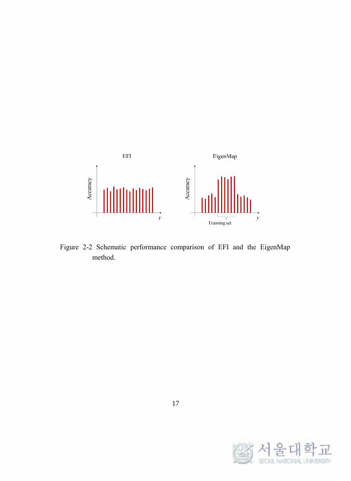
Since both the EFI method and the EigenMap method are based on the basis
vectors of the system, they can estimate any kind of signal to some extent. However,
the difference is that the EFI method shows good estimation capability in general,
while the EigenMap method shows very accurate results for system behavior similar
to the training data, but is less accurate for other cases. This difference is
schematically shown in Figure 2-2. The choice of the methods could be determined
according to the operating condition of the system. If the system is operating under
restricted conditions, the EigenMap method could give accurate estimation results
with a smaller number of sensors. On the other hand, if the operating conditions are
not restricted to particular operating conditions, the use of the EFI method will give
better results.
17
Figure 2-2 Schematic performance comparison of EFI and the EigenMap
method.

18
Chapter 3. Stochastic Sensor Network Design
This Chapter discusses optimal sensor placement under parametric uncertainties.
The EFI method is reformulated from the stochastic view. The resultant formula for
stochastic EFI contains the deterministic term, which has the same form with the
deterministic EFI, and an additional stochastic term. The stochastic term can be
calculated with the help of the stochastic finite element method (SFEM). The
developed method is expanded to the energy-based OSP method.
3.1 Stochastic Finite Element Method
3.1.1 Principle of Stochastic Perturbation
The uncertainty of the OSP problem can be quantified with probabilistic moments
using SFEM. In this research, the perturbation-based method is adapted to calculate
the probabilistic moments [25-28]. The perturbation-based method finds the
stochastic moments of the target function by expanding the state function of the
random variables using the Taylor series. That is, for a random variable, b, the Taylor
series expansion of state function f(b) is
0
1
1 ( )( ) ( )
!
nn n
nn
f bf b f b
n b
(10)

19
where f 0 denotes the function value evaluated at the expectation b0; ɛ∆b = ɛ (b - b0)
is the first variation of b for a perturbation with a given small parameter ɛ. The
expectation of the target function with the probability density p(b) is
0
1
[ ( ); ] ( ) ( )d
1 ( )( )
!
nn
nnn
E f b b f b p b b
f bf b
n b
(11)
In the last equation, the mth central moment, μm is
( ( ); ) ( ( ) ) ( )dm
m f b b f b E p b b
. (12)
For example, the second-order central moment, also called variance, up to fourth
order accuracy is
22 2 32 4
2 42 3
1 1Var( ( )) ( ) ( )
4 3
f f f ff b b b
b bb b
(13)
For the higher-order moments up to higher-order accuracy, refer to [26]. The nth
order partial derivatives in the expectation and the moment equation are obtained by
numerically solving the variational formulation of the linear structural system
equation.
3.1.2 Stochastic Eigenvalue Problem

20
The stochastic characteristics of the mode shape matrix are obtained by solving
the eigenproblem of the mass and stiffness matrix. The expanded mass and stiffness
matrix by the Talyor series is substituted into the variational formulation and the
same order of perturbation ɛ is equated to have the following eigenvalue problem
[25, 29]:
Zeroth order:
0 0 0 0 0 0 0 0( ) ( ) ( ) ( ) 0K b b M b b (14)
First order:
0 0 0 0 0 0 , 0 , 0 , 0 0 0 0 0 , 0 0 0( ) ( ) ( ) ( ) ( ) ( ) ( ) ( ) ( ) ( )K b b M b b K b b M b b M b b
(15)
where M and K are the mass and stiffness matrix; λβ and ϕβ are the system eigenvalue
and the corresponding eigenvector; and the superscript (·),ρ indicates the first-order
derivative with respect to the random variable bρ. To know the statistics of the
eigenvalue and eigenvector, refer to [25]. Then, the first-order accurate cross-
covariance for the α-th component of the αp-th eigenvector and the β-th component
of the βp-th eigenvector is calculated as

21
0 0 , ,
( ) ( ) ( ) ( )Cov( , ) Cov( , )p p p p
b b
(16)
This stochastic moment is used for the stochastic EFI in the following section.
3.2 Stochastic Effective Independence Method
The EFI method is analyzed considering the parametric uncertainty. In Eq.(1) the
uncertainty of the output y comes from the measurement noise w. However, in reality,
the target mode shape Φ also has uncertainty that comes from the parametric
uncertainties, such as Young’s modulus. Thus, a random sample of Φ can be
expressed as the sum of mean Φm and residual Φv,
m v Φ Φ Φ (17)
Then Eq.(1) is described as
m v y Φ q Φ q w (18)
In this equation, Φm is deterministic, and Φvq+w is random. Comparing Eq.(18)
with Eq.(1), Φvq+w can be interpreted as the measurement noise. Hence, the noise
variance term of the initial FIM in Eq.(4) is no longer considered constant. Therefore,
the FIM is affected by the variance of Φ. From this perspective, we see that a DOF

22
that largely contributes to the linear independence of the mode shapes cannot always
be included in the set of sensor locations if its variance is considered. There might
be a balancing point between linear independence and variance that maximizes the
determinant of the FIM, on average.
To analyze the effect of the uncertainty of the mode shape matrix and to evaluate
the optimal sensor location, the mode shape matrix is expressed as in Eq.(17). Then,
the FIM is
T
s m v m v Q Φ Φ Φ Φ (19)
Instead of integrating the randomness into the measurement noise, the
randomness is maintained in the mode shape matrix to keep the same form of the
FIM with the deterministic EFI method. In this case, the variance of noise is
stationary and hence ignored in the FIM. The fractional eigenvalue matrix is obtained
as
1
E m v m v m v m v m v
F Φ Φ ψ ψ Φ Φ ψ ψ λ λ (20)
The eigenvalue and the eigenvector of Qs are expressed as (λm + λv) and (ψm +ψv),
respectively, since they are also random from the randomness of Qs. To reduce the
complexity, those eigenpairs are approximated using the first-order, perturbation-

23
based stochastic finite element method [25], which is obtained by solving the
eigenproblem:
0 0s m m
Q λ I ψ (21)
Q0s is the value evaluated at the expectation of the random variable. Then, the
fractional eigenvalue matrix becomes
1
E m v m m v m m
F Φ Φ ψ Φ Φ ψ λ (22)
Figure 3-1 shows the schematic representation of Eq.(22). A sample of the row
of Φ has a probabilistic distribution where its mean is located at Φm and its residual
is Φv. This row vector of the mode shape matrix is transformed by the mean
eigenvector ψm to the eigenvector space, called absolute identification space. Then,
the magnitude of the transformed vector is measured by the term-by-term
multiplication and normalized by the mean eigenvalue λm to compare the
transformed vector based on the same measure.

24
Expanding and taking expectation of FE becomes
Figure 3-1 Transformation of the row of the mode shape matrix (Φm) to the
absolute identification space.

25
1
1 1
1
E E
2E
E
E m v m m v m m
m m m m m m m v m m
v m v m m
F Φ Φ ψ Φ Φ ψ λ
Φ Ψ Φ Ψ λ Φ Ψ Φ Ψ λ
Φ Ψ Φ Ψ λ
(23)
The expectation of the second term in Eq.(23) is
1 1E Em m v m m m m v m m
Φ Ψ Φ Ψ λ Φ Ψ Φ Ψ λ (24)
The expectation of Φv is zero; with the assumption of a symmetric distribution of
Φ, Eq.(24) vanishes. The expectation of the last term in Eq.(23) is
, , , ,E Cov ,v m v m v ik m il m kj m ljijk l
Φ Ψ Φ Ψ (25)
If there is no correlation between the element of Φv, (for example, Young’s
modulus of a truss element is not affected by, or independent from the other
elements), Eq.(25) becomes
E Varv m v m v m m Φ Ψ Φ Ψ Φ Ψ Ψ (26)
In Eq.(26), the Var[Φv] indicates the elementary variance of Φv. In conclusion,
the expectation of FE is
1 1E +VarE m m m m m v m m m
F Φ Ψ Φ Ψ λ Φ Ψ Ψ λ (27)

26
In this equation, the first term is the same as the deterministic EFI evaluated at
the expectation, and the second term contains the effect of the variance on FIM.
Finally, the summation of the column vector of the E[FE], the stochastic effective
independence distribution ED,SEFI, represents the contribution of a DOF to the
determinant of the FIM.
1 1
, E +VarD SEFI E m m m m m v m m m
E F Φ Ψ Φ Ψ λ 1 Φ Ψ Ψ λ 1 (28)
Then, the rest of the procedure is identical to the procedure used for deterministic
EFI, described in Section 2. That is, the DOF with the lowest value of ED,SEFI is
removed at each iteration until the number of the remaining DOFs reaches the given
number of sensors.
As an example, consider the following probabilistic mode shape matrix Φ
composed of the mean Φm and the deviation Φv. The elements of the mode shape
matrix have the probabilistic distribution function following the Gaussian
distribution, where its mean and deviation are
5 1
E 4 4
1 1
m
Φ Φ and
2 2
2 2
2 2
0.5 0.1
Var Var 0.4 0.4
0.3 0.3
v
Φ Φ .

27
Each row and column of Φ corresponds to the DOF and the mode shape,
respectively. Transformation of each row of Φ to the absolute identification space
generated by the mean eigenvectors ψm of the FIM is shown in Figure 3-2. In the
figure, the transformed vector Φiψm from the ith row of Φ by the conventional
deterministic approach is indicated by the arrow named ρi,det. Furthermore, to
compare this deterministic result with the stochastic result, 1,000 samples of Φ were
generated according to its PDF and transformed to the eigenvector space of the FIM.
The result is shown as clustered points around each tip of the arrow, and named ρi,MCS.
From Eq.(6), the squares length of the transformed vector is related to the linear
independency, and it will be affected by the randomness as observed in the figure.
To see this, the effective independence distribution, ED is calculated using three
methods, namely, the deterministic method, the mean value of MCS method, and the
proposed stochastic EFI method; these methods are, respectively
,det
1
0.9412
0.0588
D
E , ,MCS
0.9876
0.9341
0.0783
D
E , and ,SEFI
1.0022
0.9434
0.0787
D
E
The elements of ED represent the contribution of corresponding DOFs to the
linear independence. From the 3rd row of ED,det, and ED,MCS, we see that the
randomness truly affects the contribution of DOFs to the linear independence, which
could change the selection of the sensor. Also, we see that the randomness is

28
accurately captured by the stochastic EFI method. Hence, the stochastic EFI method
will help to select the optimal sensor location under uncertainty.
The result by MCS in the example is used as a benchmark test to compare the
accuracy of the stochastic property by the proposed method. However, the MCS
method cannot be applied in this way because the stochastic property for the mode
shape matrix is not known; it is computationally expensive to obtain it at every
iteration of the EFI method. Instead, the MCS method is used to generate random
samples, and to select the sensor locations for each samples [20]. Then, the most
frequently selected sensors out of all samples are determined as the final sensor
locations. This approach, however, contains the possibility that sensors with a low
contribution to the linear independence are selected instead of those with a higher
one. This will be shown and discussed in Section 3.4.

29
Figure 3-2 Example of the transformation of the row of the mode shape matrix
(Φm) to the absolute identification space. The arrow indicates the
deterministic transformation and the point cluster indicates the
probabilistic transformation generated by the MCS method.

30
3.3 Energy-Based Stochastic EFI Method
The EFI method is expanded to the energy-based method by adapting the mass
and stiffness matrix into the FIM. The FIM is then expressed as
T
E Q Φ WΦ (29)
If the weight matrix W is the mass matrix, as in Eq.(7), it is the kinetic energy
equation; if W is the stiffness matrix, it is the strain energy equation. For the energy
method, the FIM is newly defined as
T whereE Q ζ ζ ζ CΦ (30)
Here, the weight W is decomposed by the Cholesky decomposition as W=CTC.
The decomposition of the weight matrix can be executed in several different ways,
such as 𝐖 = √𝐂√𝐂. To check other decomposition options and their effects on the
results, refer to [19].
Once the FIM is defined, the rest of the procedure is identical to the EFI method.
The only difference is that Φ is replaced by ζ. Then, the mean and the covariance of
ζ are calculated as
m mζ CΦ (31)

31
T
, ,Cov Covv ij v ij ζ C C (32)
The resultant expectation of the fractional eigenvalue matrix FE for the energy-
based method is
1 1E +VarE m m m m m v m m m
F ζ Ψ ζ Ψ λ ζ Ψ Ψ λ (33)
From the equation above, the summation of the column generates the effective
independence distribution vector for each element indicates the contribution of a
DOF to the linear independence. The DOF that has the lowest contribution to the
linear independence is eliminated. The whole procedure is repeated until the number
of DOFs meets the given number of target modes.
3.4 Case Study
The method suggested in the previous section is demonstrated here by applying
it to a two-dimensional truss bridge whose Young’s modulus is set to be a random
variable. The result is compared with the existing sensor selection method that is
based on Monte Carlo simulation.

32
3.4.1 Truss Bridge Structure
To demonstrate stochastic EFI, a truss bridge structure was modeled by the finite
element method. It is shown in Figure 3-3. The truss bridge is composed of the 41
truss elements and 18 nodes. Each node has two DOFs that describe x- and y-
direction displacement, respectively. The x-direction DOF for the nth node is
numbered 2(n-1), and the y-direction DOF is numbered 2n. The DOFs of both
directions at node 1 and in the y-direction at node 17, that is, DOFs 1, 2, and 34 are
constrained. The cross-sectional area of the truss element is 5×10⁻³ m2, and the mass
density is 2500 kg/m3. The Young’s modulus is set to be a random variable that has
the truncated normal distribution with mean 70 GPa. Three different standard
deviations of the Young’s modulus are simulated for verification of the suggested
method; 0.0.5×70 GPa, 0.1×70 GPa, and 0.2×70 GPa.
In this case study, the target modes are set to be the first ten modes to represent
the overall structural behavior. However, for the purpose of structural health
monitoring, one can choose other modes that are useful for a specific fault. The first
4 modes are shown in Figure 3-4, with their mean and standard deviation that are
simulated with the help of the SFEM [30, 31].

33
Figure 3-3 Two-dimensional truss bridge.
(a)
(b)
(c)
(d)
Figure 3-4 Target mode representation with mean and standard deviation: (a) 1st
mode, (b) 2nd mode, (c) 3rd mode, and (d) 4th mode.

34
3.4.2 Sensor Placement Under Uncertainty
3.4.2.1 Monte Carlo Simulation
Optimal sensor selection under parametric uncertainty was studied by Castro-
Triguero [20] for a truss bridge. The authors use Monte Carlo simulation to select
ten sensors under parametric uncertainty. The histograms of 1,000 EFI simulations
of sensor selection under three different variances of the Young’s modulus are shown
in Figure 3-5.

35
(a)
(b)
(c)
Figure 3-5 Histograms of 1,000 EFI simulations with stochastic Young’s
modulus with the mean 70 GPa: (a) the standard deviation 0.05×70
GPa, (b) the standard deviation 0.1×70 GPa, and (c) 0.15×70 GPa.

36
In Figure 3-5, when the variance of the Young’s modulus is low, the set of
selected sensors does not change much. However, as the variance increases, the
number of sensors consistently selected decreases. For example, DOF 22 is selected
for most of the simulation in the lower variance case, but as the variance increases
the selection ratio reduces gradually. In contrast to DOF 22, the increase in sensor
selection is observed for other sensors such as DOFs 16, 18, and 35. We also observe
that the selection of the DOFs around the constraint, such as the DOFs 3, 6, and 33
does not change much even with a high variance of the Young’s modulus, because
their variances are kept relatively low by the constraints. In contrast, the DOFs away
from the constraints, such as DOFs 18, 22, and 23, show less consistency in selection
even with the low variance. Similar features are observed for energy-based EFI. The
results of strain energy EFI, which uses the stiffness as a weight, are shown in Figure
3-6.

37
(a)
(b)
(c)
Figure 3-6 Histograms of 1,000 strain energy EFI simulations with stochastic
Young’s modulus with the mean 70 GPa: (a) the standard deviation
0.05×70 GPa, (b) the standard deviation 0.1×70 GPa, and (c) 0.15×70
GPa.
(c)

38
Based on the histograms, the MCS method gives the basic idea of selecting sensor
locations under parametric uncertainty. The intuitive method is to choose the 10 most
frequently selected sensors, for example, in Figure 3-5 (a) the set (3, 6, 12, 13, 14,
21, 22, 26, 30, 33) would be selected. However, this selection does not always assure
the optimal set of sensors, especially when the variance is high, because it overlooks
the correlation between the sensors. For instance, it is possible that a DOF that has
lower linear independence than the DOFs with the 10 highest linear independences
is never selected during the simulation, but that it does belong to the 10 highest
sensors on average. In the following section, the stochastic EFI indeed shows this
case, and finds the optimal sensor locations that give the highest ten linear
independences, on average.
3.4.2.2 SEFI Method
The DOFs for the sensor placement are selected using the suggested stochastic
EFI for the truss bridge with three different variances. The set of sensors selected
using the stochastic EFI are shown and compared with the deterministic EFI and
MCS results in Table 3-1.
The performance of each of the three approaches is compared by calculating the
determinant of the FIM with respect to the randomly generated 1,000 truss bridges

39
according to the random property. The histograms of the determinant of the FIM are
shown in Figure 3-7 and their mean value is found in Table 3-3.

40
Table 3-1 The set of 10 sensors selected by EFI using the deterministic EFI, MCS,
and stochastic EFI
Std. of Young’s
modulus, GPa Method Sensor set
Mean det(ΦTΦ)
(log scale)
0.05×70
DEFI
3, 6, 12, 13, 14, 21, 22, 26, 30, 33 -107.6160 MCS
SEFI
0.1×70
DEFI 3, 6, 12, 13, 14, 21, 22, 26, 30, 33 -107.6603
MCS 3, 6, 12, 13, 18, 21, 22, 26, 30, 33 -107.7878
SEFI 3, 6, 12, 13, 14, 21, 22, 26, 30, 33 -107.6603
0.15×70
DEFI 3, 6, 12, 13, 14, 21, 22, 26, 30, 33 -107.7277
MCS 3, 6, 12, 13, 18, 22, 23, 26, 30, 33 -107.8264
SEFI 3, 6, 12, 13, 14, 21, 22, 26, 30, 33 -107.7277

41
(a) (b) (c)
(d) (e) (f)
(g) (h) (i)
Figure 3-7 Determinant of the Fisher information matrix by (a) EFI with standard
deviation of 0.05×70 GPa , (b) MCS with standard deviation of
0.05×70 GPa , (c) stochastic EFI with standard deviation of 0.05×70
GPa , (d) EFI with standard deviation of 0.1×70 GPa , (e) MCS with
standard deviation of 0.1×70 GPa , (f) stochastic EFI with standard
deviation of 0.1×70 GPa , (g) EFI with standard deviation of 0.15×70
GPa , (h) MCS with standard deviation of 0.15×70 GPa , and (i)
stochastic EFI with standard deviation of 0.15×70 GPa.

42
For the case of a low variance of Young’s modulus, the selected sensor sets are
not different for between MCS and stochastic EFI. This is because the selected 10
sensors overwhelm the other sensors (Figure 3-4(a)); thus, it is not difficult to choose
the sensors using either method. Also, the results are the same with deterministic EFI
because of the low variance. However, as the variance increases, the number of
overwhelming sensors decreases (Figure 3-4(b)), and the selection becomes
confusing when the frequencies in the histogram are similar. However, in this case,
the selection of higher frequency does not always give the best result, as mentioned
before. For example, in the mid-variance case, the sets selected by the MCS and the
stochastic EFI are the same, except for DOFs 14 and 18. Although DOF 14, selected
by stochastic EFI, has less frequency than DOF 18, selected by the MCS as in Figure
3-4(b), det(ΦTΦ) with DOF 14 is higher as shown in Figure 3-7 (b) and in Table 3-3.
This phenomenon is intensified as the variance grows, the number of overwhelming
sensors decreases, and the difference between the MCS and the stochastic EFI results
increases. This is observed in the high-variance case. The number of different
sensors between the sets selected by MCS and stochastic EFI increased to two, which
are DOF (18, 23) for MCS and (14, 21) for stochastic EFI.
Another aspect to notice is that deterministic EFI gives the same sensor sets as
stochastic EFI. This is because deterministic EFI is basically the zeroth order
approximation of stochastic EFI. However, deterministic EFI does not always give

43
the same results as stochastic EFI, if the variance can affect the results more. This
will be shown in the results of the following energy-based EFI method. Also, note
that the determinant of FIM is decreasing as the variance increases.
The difference in the determinant of the Fisher information matrix, or the linear
independence, leads to different estimation performance. To show this, estimations
are conducted for two cases of deflection, as shown in Figure 3-8.
For those cases, the Young’s modulus of each element is set to have 15% standard
deviation from its mean, and 1000 samples are generated accordingly. The
corresponding sensor locations are found in Table 3-1. Based on the data measured
at the given sensor locations, the deflection for each sample is reconstructed using
Eq.(3). Sample estimations for both MCS and proposed method are shown in Figure
3-9. The estimated errors are calculated for 1000 samples; the average differences
are shown in Table 3-2.

44
Figure 3-8 The target deflections of a truss bridge with the mean Young’s modulus
(a) (b)
(c) (d)
Figure 3-9 The estimated deflection for a randomly generated truss bridge
generated by: (a) MCS for case 1, (b) MCS for case 2, (c) SFEM for
case 1, and (d) SFEM for case 2

45
Table 3-2 The average estimation error of MCS and SFEM for given cases
Average RMS error
Case 1 Case 2
MCS 0.0253 0.0055
SFEM 0.0109 0.0023

46
From the results, we see that the proposed method not only shows the higher
linear independence, but also it indeed gives more accurate estimation than the MCS
method.
Stochastic EFI is verified with the energy-based method. The stiffness matrix is
used for the weight matrix, W and the Cholesky decomposition is used to define the
FIM. The results are shown in Table 3-3 and the determinant of the FIM for different
standard deviations of Young’s modulus are shown in Figure 3-10.

47
Table 3-3 The set of 10 sensors selected by strain-energy-based EFI using the
deterministic EFI, MCS, and stochastic EFI
Std. of Young’s
modulus, GPa Method Sensor set Mean det(ζTζ)
0.05×70
DEFI 8, 11, 12, 16, 17, 24, 27, 28, 32, 33 4.3139×10¹⁰
MCS 7, 8, 12, 16, 20, 24, 27, 28, 32, 33 4.3066×10⁷
SEFI 7, 8, 9, 12, 20, 24, 27, 29, 32, 35 9.0426×10¹⁰
0.1×70
DEFI 8, 11, 12, 16, 17, 24, 27, 28, 32, 33 4.4851×10¹⁰
MCS 7, 8, 12, 16, 20, 24, 27, 28, 32, 33 1.5199×10⁸
SEFI 7, 8, 9, 12, 20, 23, 24, 29, 32, 35 1.5042×10¹¹
0.15×70
DEFI 8, 11, 12, 16, 17, 24, 27, 28, 32, 33 4.5497×10¹⁰
MCS 7, 8, 12, 16, 20, 24, 27, 28, 32, 33 3.7275×10⁸
SEFI 8, 11, 12, 16, 17, 24, 27, 28, 32, 33 1.3712×10¹¹

48
(a) (b) (c)
(d) (e) (f)
(g) (h) (i)
Figure 3-10 Determinant of the Fisher information matrix by (a) energy-based
EFI with standard deviation of 0.05×70 GPa , (b) MCS with standard
deviation of 0.05×70 GPa , (c) stochastic EFI with standard deviation
of 0.05×70 GPa , (d) energy-based EFI with standard deviation of
0.1×70 GPa , (e) MCS with standard deviation of 0.1×70 GPa , (f)
stochastic EFI with standard deviation of 0.1×70 GPa , (g) energy-
based EFI with standard deviation of 0.15×70 GPa , (h) MCS with
standard deviation of 0.15×70 GPa , and (i) stochastic EFI with
standard deviation of 0.15×70 GPa.

49
Unlike the EFI method, this strain-energy-based method shows different sensor
selection even in the case of low variance. This is because the stiffness matrix is the
function of the random variable, Young’s modulus, and the sensor selection becomes
more sensitive by taking it into the FIM. Note that while all the methods give
different results, stochastic EFI gives the best results among them.
Another energy-based method, the kinetic-energy-based method that uses the
mass matrix as the weight matrix, shows different sensor locations with the EFI and
strain-energy-based methods due to the targeting of different information. The
results are shown in Table 3-4. It is worth noting that the variation of sensor locations
according to the uncertainty is more comparable with the EFI method than the strain-
energy-based method. This is because the mass matrix is not a random quantity, and
does not add randomness to the kinetic energy form as the stiffness matrix does to
the strain energy form. Thus, the mode shape matrix is the only factor that affects
the result, as seen in the EFI method.

50
Table 3-4 The set of 10 sensors selected by kinetic-energy-based EFI using the
deterministic EFI, MCS, and stochastic EFI
Std. of Young’s
modulus, GPa Method Sensor set Mean det(ζTζ)
0.05×70
DEFI 8, 11, 12, 16, 17, 24, 27, 28, 32, 33 4.3139×10¹⁰
MCS 7, 8, 12, 16, 20, 24, 27, 28, 32, 33 4.3066×10⁷
SEFI 7, 8, 9, 12, 20, 24, 27, 29, 32, 35 9.0426×10¹⁰
0.1×70
DEFI 8, 11, 12, 16, 17, 24, 27, 28, 32, 33 4.4851×10¹⁰
MCS 7, 8, 12, 16, 20, 24, 27, 28, 32, 33 1.5199×10⁸
SEFI 7, 8, 9, 12, 20, 23, 24, 29, 32, 35 1.5042×10¹¹
0.15×70
DEFI 8, 11, 12, 16, 17, 24, 27, 28, 32, 33 4.5497×10¹⁰
MCS 7, 8, 12, 16, 20, 24, 27, 28, 32, 33 3.7275×10⁸
SEFI 8, 11, 12, 16, 17, 24, 27, 28, 32, 33 1.3712×10¹¹

51
The advantage of stochastic EFI does not only lie in optimal sensor selection, but
also in reducing the computational effort. Stochastic EFI requires much less
computational work than the MCS method. The MCS method generates a large
number of input samples and simulates as many times as the number of the input
samples to obtain the probabilistic characteristics of the output. Unlike MCS,
stochastic EFI with SFEM needs only one simulation to determine the stochastic
properties of the output. The computational times of both methods are compared for
the various lengths of the truss bridge in Table 3-5.

52
Table 3-5 The simulation time of MCS with 1,000 simulations and stochastic EFI for
a 2-D truss bridge
No. of truss block 6 7 8 9 10 11
MCS 3.8261 4.8313 5.6736 6.6168 7.5172 8.3789
Stochastic EFI 0.0087 0.011 0.0158 0.0121 0.0161 0.0154

53
For a six truss block sample, the MCS method with 1,000 simulations takes
almost 440 times longer than the proposed method. This computational difference
increases if the structure becomes large and complicated, as observed in Table 3-5.
As the number of the truss blocks increases, the computational time of MCS
increases, while the computational time of the stochastic EFI method remains almost
constant. If the required number of samples increases due to multiple random
variables, or a complex probability distribution, the computational difference will be
much more severe.
3.5 Conclusion
The research described in this dissertation proposed an analytic method for
optimal sensor placement under parametric uncertainty. The stochastic EFI was
derived, which is composed of the deterministic EFI and an additional random part.
With the help of SFEM, the stochastic moments required for the stochastic EFI
method are readily obtained, dramatically reducing the total computation time.
Applying the suggested method to a 2-dimensional truss bridge case study showed
the same or higher determinant of FIM on average as the MCS method, which
indicated higher linear independency between the columns of the mode shape matrix
with reduced DOFs. It also showed higher representativeness of the general vibration

54
using the information from the given locations of the sensors. For small variances of
the parameter, the selected sensor sets were the same for both methods; however, as
the variance increased, the sensor set from the suggested method showed higher
linear independence.
The proposed method was expanded to energy-based OSP methods, such as the
kinetic energy method, and the strain energy method – both originate from the EFI
method. The derivation of such methods for a stochastic case were obtained and they
were validated with the same truss bridge case study. The results show that the
suggested method shows higher linear independence.
In deriving the stochastic EFI, the symmetric probability distribution of a random
variable, and the first-order Taylor expansion for some variables were assumed. For
more accurate results, analysis of these assumptions will be required. This analysis
will be dealt with in a future study.

55
Chapter 4. Robust Sensor Network Design
This chapter proposes a sensor network design that considers possible sensor
malfunctions, and where the designed sensor network is applied for estimation of the
temperature distribution of a Li-ion battery pack. Section 4.1 describes the
development of the thermal model for the battery pack to extract the basis matrix. In
the next section, an objective function is proposed and solved using the genetic
algorithm for the optimization problem that maximizes the linear independence of
the system under malfunction. In the final section, the proposed method is validated
for various heat conditions.
4.1 Battery System
4.1.1 Battery Pack Overview
Here, a thermal simulation model for a battery pack is developed using the
lumped parameter. The battery pack is composed of 50 number 18650 cylindrical
cells (ICR18650B4, LG Chem.) with 2600mAh capacity, and 3.7V nominal voltage.
The geometry of the battery pack is shown in Figure 4-1(a) and its lumped finite
element model is shown in Figure 4-1(b). Each cell is represented as a node and it is
connected with the surrounding cells by thermal resistance. At each cell, heat is

56
generated by electrochemical reactions. The heat is transferred to the surrounding
cells by conduction and to the air by convection. The energy balance equation for
the ith cell in the battery pack is as follows [32-34]:
,( ) ( )i
h t i j i amb i
j
dTC R T T Q h T T
dt (34)
where Ch is the heat capacity of the cell, Ti is the temperature at the ith cell, and Tj is
the cell around the ith cell, Tamb,i is the ambient temperature, t is the time, Rt is the
thermal resistance between cells, �̇� is the heat generation rate, and h is the heat
transfer coefficient. The rationale for the simplicity of this lumped model is based
on three perspectives. First, for practical use in a management system, the
computational requirement needs to be small. Second, the errors that could occur in
the model can be compensated for through the measurements. In addition, the small
size of the 18650 cells with small Biot numbers allow us to assume a small
temperature variance in the cell [34, 35].

57
(a)
(b)
Figure 4-1 (a) Battery pack geometry, and (b) the lumped parameter model.

58
4.1.2 Heat Generation Model
During charging and discharging, heat is generated inside the cell. There are
several heat sources, such as irreversible ohmic heating, reversible entropic heat,
heat from phase change of the active materials, and the heat of mixing [34-36]. In
this study, two dominant heat sources, irreversible ohmic heating and reversible
entropic heating are considered [32]. The heat generation rate is given as
2 OCVdVQ I R IT
dT (35)
where I is the input current, R is the impedance of the cell, and VOCV is the open
circuit voltage. The first term is the ohmic heating and the second term is the entropic
heat. Since the impedance is dependent on the state-of-charge (SOC), the hybrid
pulse power characterization (HPPC) test is performed to obtain the SOC and
impedance relationship [36, 37]. Figure 4-2(a) shows the HPPC test profile. The
discharge pulse is applied for 10 seconds followed by 1C discharge to reduce the
SOC by 10%. By repeating this procedure, the impedance at every 10% SOC can be
calculated. At the last step, the discharge current is half of the others in order not to
violate the cut-off voltage. Therefore, the impedance obtained at this step is for 5%
SOC. The impedance is simply calculated as V/I at the beginning of discharging the
current. The impedance to the SOC is shown in Figure 4-2(b). Also, dVOCV/dT for

59
entropic heat is obtained as a function of SOC according to [32, 36]. The voltage of
the battery at rest is measured with the change of the temperature at a certain SOC
level. The equation VOCV=A+BT+Ct is fitted to the measured voltage, then the
coefficient B is dVOCV/dT at a given SOC. The test profile at SOC 0% is shown in
Figure 4-3(a) as an example. Similarly, dVOCV/dT at different SOC levels is obtained,
and the results are shown in Figure 4-3(b).
Finally, for calculation of the SOC during operation, the coulomb counting
method given in Eq.(36) is used [38].
1
i
k k k
n
tz z I
C
(36)
In the above equation, k is the time index, zk is the SOC at time index k, ηi is the
Coulombic efficiency, Δt is the time difference between k+1 and k time indices, Cn
is the nominal capacity of the cell, and Ik is the input current. With the impedance,
dVOCV/dT, and SOC as a lookup table, the heat generation can be calculated.

60
(a)
(b)
Figure 4-2 (a) HPPC test profile, and (b) impedance values at SOC levels.

61
(a)
(b)
Figure 4-3 (a) Entropic heat test profile and (b) dVocv/dT.

62
4.1.3 Model Calibration and Validation
The model parameters of a single cell, the heat capacity, and the heat transfer
coefficient, are calibrated and validated with experimental results. All the
experiments are conducted using the Maccor Series 4000 for dis/charging, and the
heat chamber for controlling the ambient conditions. First, for model calibration, the
temperature under a 1C discharging condition is obtained and used for target vector
to optimize the model parameters. The optimized heat capacity and heat transfer
coefficient are 69.43 J/K, and 0.1555 W/m2K, respectively. The measured and the
simulated temperatures are shown in Figure 4-4. The model is then validated with
the urban dynamometer driving schedule (UDDS) current profile, which is shown in
Figure 4-5(a). The UDDS profile and 10% SOC discharging is performed
alternatively until the SOC is near zero, then the charging process follows. The
measured and the simulated temperatures for this current profile are shown in Figure
4-5(b). The simulated result shows good agreement with the measured temperature
during the discharge. The temperature at charging deviates a bit from the measured
one, because the impedance used is obtained from discharging pulse. For better
results during charging, the impedance needs to be calculated using the charging
impulse.

63
Figure 4-4 The measured and simulated temperatures under 1C (=2.6A)
discharge current.

64
(a)
(b)
Figure 4-5 UDDS test results: (a) UDDS current profile, and (b) the measured
and the simulated temperature.

65
4.2 Robust Sensor Network Design
Using the parameters found by the single cell experiments, the pack model is
constructed and simulated. Various scenarios that cover possible realizations of the
battery pack are generated as a training data set. One of the scenarios is shown in
Figure 4-6. It is obtained from the constant current discharge condition. The figure
on the left is the temperature change of the cells across time and the figure on the
right is the temperature distribution of the pack at a certain time (83 min.). From the
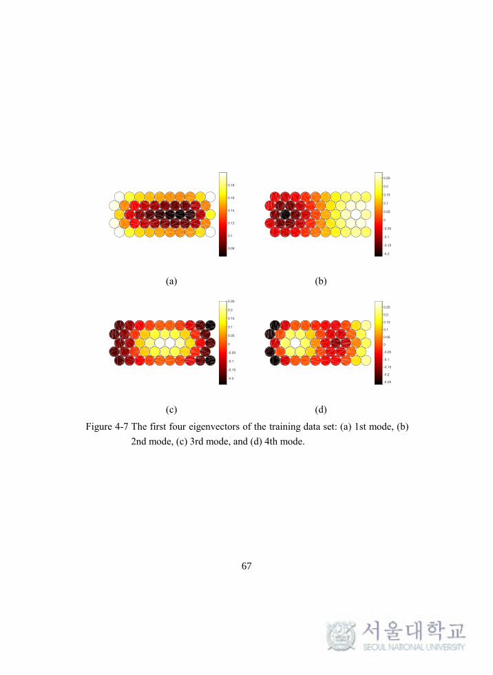
training data set, the covariance matrix is found as in Eq.(9), and the eigenanalysis
of the covariance matrix gives the basis matrix, Φ. The first four bases are shown in
Figure 4-7. This basis matrix will be used to find the optimal sensor locations.

66
(a)
(b)
Figure 4-6 The temperature distribution of a battery pack under constant current:
(a) temperature change across time, and (b) the temperature
distribution at 83 min.
67
(a) (b)
(c) (d)
Figure 4-7 The first four eigenvectors of the training data set: (a) 1st mode, (b)
2nd mode, (c) 3rd mode, and (d) 4th mode.

68
The object of selecting sensor locations is to maximize the determinant of the
Fisher information matrix with the (k×k) matrix, Φs. It is the matrix that (n-k) rows
and columns are eliminated out of the (n×n) mode shape matrix, Φ. Therefore, the
selections must be made for both rows and columns. The rows are the candidate
location of sensor placement and will be decided by the genetic algorithm later. The
columns are the mode shape vectors, and will be selected as the mode shapes
corresponding to the k lowest eigenvalues of Φ. The choice of low-frequency mode
shapes is adequate to represent the general behavior of the system. If the operating
condition of the system is restricted so that the dominant mode shapes are known by
and large, then the selection of these mode shapes will bring better estimation under
that condition. However, this study focuses on the estimation of an arbitrary loading
condition and so we stay with k lowest mode shapes.
The choice of rows, or sensor locations, is considered in two aspects. First, the
linear independence needs to be high enough to reconstruct the whole thermal map
out of the measured signal. Second, for the sensor network to be robust, the sensor
network needs to keep its functionality under latent sensor failure. Then, the
objective function and the constraints are formulated as follows:

69
T
1 1 1
T T
1 1 1 1
Maximize:
( ,..., ) E[det( [{ ,..., } \{ };1,..., 1] [{ ,..., } \{ };1,..., 1])]
Subject to :
det( [ ,..., ;1,..., ] [ ,..., ;1,..., ]) det( [ ,..., ;1,..., ] [ ,..., ;1,.
k k j k j
opt opt opt opt
k k k k
f i i i i i k i i i k
i i k i i k i i k i i
Φ Φ
Φ Φ Φ Φ .., ])k
(37)
where k is the given number of sensors, Φ[i1,…, ik; j1,…, jk] is the submatrix of Φ
formed from the rows {i1,…, ik}and columns {j1,…, jk} such that il∈, 1≤ il ≤n, and
il ≠ im. As mentioned before, the mode shapes are preselected as the first k mode
shapes. The random variable for calculating the expectation in the objective function
is ij which is an element in {i1,…, ik}. Therefore, the objective function indicates the
average linear independence of the system when a sensor fails. The constraint is set
to satisfy a certain performance. That criterion is determined based on the sensor
placement result without considering the failure. The iopt is the optimal sensor
location when failure is not considered. The coefficient α determines the
performance criterion.
Since the sensor placement is the combinatorial problem that selects a given
number of sensors k out of n candidate locations, the integer valued optimization
method is required. Integer valued optimization is a non-convex problem that cannot
be solved by gradient-based optimization. Thus, in this study, the genetic algorithm
is adopted to find the sensor location giving the best linear independence of the

70
system. The genetic algorithm is a sampling-based optimization algorithm inspired
by biological evolution. It generates initial random samples (or population) and pass
them to the next generation with modification. The modification contains crossover,
mutation, and selection that are based on the evaluation of the objective function for
the samples. As the generation goes on, the optimal evolution is found as in natural
selection [39]. The sensor locations found by the genetic algorithm are shown with
the sensor network design that does not consider sensor failure in Figure 4-8.

71
(a)
(b)
Figure 4-8 The sensor locations: (a) Optimal sensor placement (OSP), and (b)
the robust optimal sensor placement.

72
4.3 Case Study
The estimation accuracy with and without considering failure of sensors is
validated for three test sets. The results are compared with the other sensor network
designs; one that does not consider the failure of sensors and another one that uses
duplicated sensors for reliability.
4.3.1 Case 1: Different Heat Generation for the Cells
Each cell that makes up the battery pack has a different specification due to
manufacturing tolerances and different degradation rates during operation. The first
test set is generated to emulate this variation of the cells. The difference in cell
specifications emerges as the different heat generation rate. Therefore, each cell is
assumed to be discharged with a constant current where the amplitude is realized
from the normal distribution N(2.6, 0.26). The temperature change is shown in
Figure 4-9(a) and the temperature distribution at 83 min. as shown in Figure 4-9(b)
is set as the target temperature distribution to be estimated.
The temperature estimations provided by the existing optimal sensor placement
(OSP) method and the proposed robust optimal sensor placement (ROSP) method
are compared in Table 4-1. Under normal conditions, both the OSP and the ROSP

73
methods show accurate estimation results of less than 1°C. Although OSP should
have the best estimation result in general, it need not be the best estimation for all
cases. This is why ROSP has slightly higher accuracy than OSP for the given case,
even though it is not the best sensor network design for the given number of sensors.
The accuracy of the estimation decreases as one of the sensors fails. However, the
accuracy drop of ROSP is less than that of OSP. Especially when the malfunction
occurs on sensor 3 the accuracy drops are severe, but ROSP has less of an accuracy
drop than OSP. The same is also true for other cases, except sensors 5 and 7. The
results of ROSP with a malfunction of sensor 5 and 7 are also comparable with OSP.
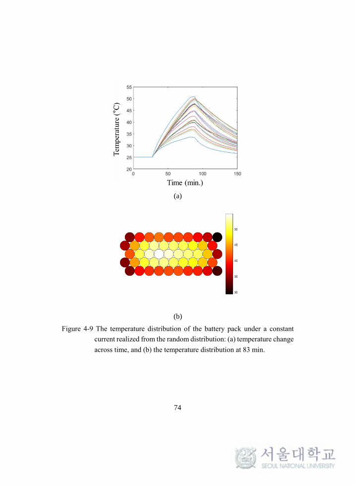
74
(a)
(b)
Figure 4-9 The temperature distribution of the battery pack under a constant
current realized from the random distribution: (a) temperature change
across time, and (b) the temperature distribution at 83 min.

75
Table 4-1 The RMS error of OSP and ROSP methods for case 1
Estimation error (RMS)
Failed sensor No. OSP ROSP
Normal 0.3311 0.5161
1 2.7575 1.4072
2 4.4064 1.2929
3 17.1811 7.6999
4 1.7658 1.6222
5 2.0477 1.974
6 4.8249 2.7842
7 1.6839 1.5953
8 1.9328 1.1974
Mean error for failure 4.57 2.45

76
4.3.2 Case 2: Forced Convection
The second case is designed to imitate a battery pack with a cooling system. The
battery pack is cooled down by forced convection that comes from the left side of
the battery pack by a set different heat transfer coefficient for each cell. The
simulation result is shown in Figure 4-10. As expected, the cells near the air inlet
and the circumference of the pack have a lower temperature than the others.
The estimation results for normal and malfunction conditions are shown in Table
4-2. Similar to what was observed in case 1, both OSP and ROSP methods give
accurate estimation results in normal conditions; however, the accuracy drops with
a sensor malfunction. The accuracy drop for the ROSP result is less than the accuracy
drop for OSP.
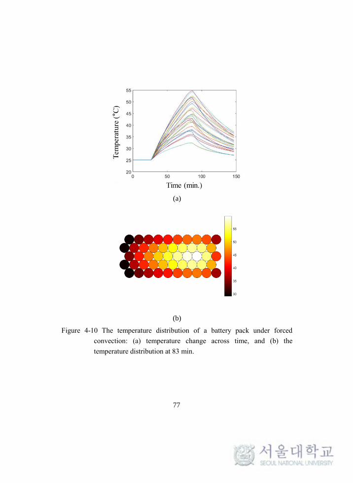
77
(a)
(b)
Figure 4-10 The temperature distribution of a battery pack under forced
convection: (a) temperature change across time, and (b) the
temperature distribution at 83 min.

78
Table 4-2 The RMS error of OSP and ROSP methods for case 2
Estimation error (RMS)
Failed sensor No. OSP ROSP
Normal 0.2658 0.3369
1 3.0945 1.3521
2 5.3976 1.5131
3 20.213 8.2920
4 1.9524 1.7199
5 2.3377 2.0404
6 5.5522 2.8814
7 1.8372 1.5646
8 2.1750 1.1891
Mean error for failure 5.32 2.57

79
4.3.3 Further Discussion on the Result
This section discusses how two aspects of sensor network design affect the results,
specifically, 1) the number of sensors and 2) the selection of mode shapes. First, the
impact of the number of sensors is tested by comparing the estimation error along an
increasing number of sensors. For case 1 and 2, Table 4-3 shows the relationship
between the differing number of selected sensors and the estimation error.
Naturally, as the number of sensors increases the estimation becomes more
accurate. Because the number of sensors is the same as the available mode shapes
used for estimation, the more sensors used, the accurate the estimation becomes.
Another thing to note is that any particular sensor network with a smaller number of
sensors is not a subset of a larger sensor network. Thus, the selection of the sensors
cannot be conducted in a consecutive manner; rather, it should be conducted for each
case.

80
Table 4-3 Sensor placement corresponding to the number of sensors and estimation
accuracy
No. Sensor Sensor Placement Estimation Error
Case 1 Case 2
5 1, 10, 22, 24, 28 1.9494 2.0523
6 1, 10, 22, 23, 26, 29 1.0888 1.0957
7 1, 10, 22, 24, 27, 29, 32 1.1843 1.1892
8 1, 10, 22, 23, 27, 29, 32, 36 0.3311 0.2658
9 1, 10, 12, 22, 23, 24, 27, 29, 36 0.1491 0.1490
10 14, 20, 22, 23, 25, 28, 32, 37, 41, 50 0.1148 0.1145
11 4, 11, 14, 20, 22, 23, 25, 27, 28, 32, 50 0.0512 0.0511

81
The second aspect that affects accuracy is the selection of the mode shapes. In
the previous study, the mode shapes were successively selected, from the low-order
mode shape to the higher order. This way of selecting sensors is for general
estimation of the system. However, if the system behavior is confined to a certain
range of the domain, estimation accuracy can be enhanced by using the dominant
mode shapes in that range. This is verified for case 1 by comparing the results with
different mode shapes; one with the low-order mode shape and the other with the
dominant mode shape. The result is shown in Table 4-4.
Two things can be observed from these results. First, the estimation accuracy is
enhanced by choosing a different mode shape. Although the increase in accuracy
observed in this example is not significant due to the small difference between the
dominant mode shapes and low-order mode shape, if there are other cases that
deviate from the orderly selected mode shape the difference will increase. Second,
the sensor locations change as the selected mode shapes are changed. This is because
the Fisher information matrix depends on the given mode shape. For this case, it is
obvious to find the dominant mode shape, so the sensor network for that specific
case is easily found. However, if the cases extend over a wider range, finding the
dominant mode shape should be carefully investigated; which will be left for future
research.

82
Table 4-4 Sensor locations and the estimation accuracy for different mode shapes
Dominant mode shape Low order mode shape
mode shape 1, 2, 3, 4, 5, 6, 8, 33 1, 2, 3, 4, 5, 6, 7, 8
Sensor locations 1, 4, 12, 20, 22,
23, 26, 28, 41, 50
14, 20, 22, 23, 25,
28, 32, 37, 41, 50
RMS error 0.2854 0.3311

83
4.4 Conclusion
In this study, we proposed a robust sensor network design that sustains estimation
accuracy under failure. We defined the objective function and the constraint for this
purpose. The optimization problem was solved by the genetic algorithm. The
selected sensor locations were used to reconstruct the temperature distribution of
various cases. The estimation results were compared with the other sensor network
designs; one was the existing sensor placement method that focuses on accuracy and
the other was to use duplicated sensors for robustness. The results show that the
proposed method has estimation capability that is comparable to the existing optimal
sensor design and that the proposed method has higher reliability than observed
using duplicated sensors.
The proposed method is advantageous for practical use in temperature estimation
for a battery pack. By combining the model and the measured data, it captures both
the computational efficiency and the estimation accuracy. In practice, such as in the
case of a battery management system in an electric vehicle, computational efficiency
is an important issue. Thus, a complicated model requiring heavy computation
cannot be used in spite of its accuracy in estimation. In contrast, the simple model is
free from the computational burden; however, it is less accurate. The proposed
method requires only a small memory to save the basis matrix and the capability to

84
calculate the matrix product; inaccuracy is compensated by the measured data and
thus, it is suitable for practical use. The use of sensors only to obtain the temperature
distribution of the battery pack is not practical because of the cost and the potential
for sensor malfunctioning.
Another benefit of the proposed method lies in the sustainability of the sensor
network under failure. The sensor network contributes to protect the system as a part
of PHM; however, the sensor network itself is vulnerable to failure. Nevertheless,
developing another protective system for the sensor network is not a good solution
because it requires redundant cost. In this situation, the proposed sensor network
design could be a solution because it does not require an extra system, while it does
maintain a certain degree of performance under failure. Unlike the PHM, which tries
to prevent failure, the proposed design allows the failure and gains time to take care
of the failure.
In this study, the sensor locations were found through the optimization method,
but it has several shortcomings. It requires significant computational resources to
find the optimal solution. Also, to find the proper solution, proper setting of the
optimization parameters is important. The genetic algorithm and the other sampling-
based optimization methods are known as the global optimization methods; however,
their solution depends on the optimization parameters and thus they do not always

85
give a global optimization solution. Hence, to reduce the computational cost, an
analytic solution is required. This will be addressed in future research.

86
Chapter 5. Contributions and Future Work
5.1 Contributions and Impacts
The work presented in this dissertation focuses on sensor network design for
prognostics and health management (PHM). As the beginning step of PHM, the
sensor network design has a profound effect on the overall successful
implementation of PHM. One of the principal problems in sensor network design is
how and where to put the limited number of sensors on the system to have the best
information we want to measure. One important property in the sensor network
design is the linear independence. The basis vectors of the finite element model that
compose an arbitrary behavior of the system, are linearly independent if the signal
corresponding to each degree-of-freedom (DOF) is known. However, the limited
measure of the system only gives partial information on some measured DOF, as a
result, the linear independence between the measured DOF is no longer guaranteed.
Since this linear independence determines the representability of the basis vectors
for the system, the purpose of the sensor network design becomes to find the
locations that make the basis vectors as linearly independent as possible. The
maximization of linear independence is considered mainly in two different aspects;
it has the following contributions:

87
Increase in estimation accuracy of sensor network design under system
uncertainty
The first research thrust proposes a method to maximize linear independence
under system uncertainty. The system in practice always has uncertainty, and the
sensor network design will be different from the deterministic solution. To find the
optimal sensor network design that considers system uncertainty, the deterministic
approach of the sensor network design is modified to its stochastic version. The
proposed method is validated using the truss bridge structure, and the results are
compared with another stochastic approach, the Monte Carlo simulation method.
The results of the research show higher linear independence on average, which
means higher representability of the system than observed in the Monte Carlo
simulation.
Reduced Computational Cost
By formulating the explicit form of the sensor network design algorithm, the
computational cost is greatly reduced. The typical approach to solve the stochastic
problem is to use Monte Carlo simulation. However, this sampling-based method
generates a large amount of samples and evaluates the system response with respect
to the samples; hence, it suffers from a significant computational burden. In contrast,

88
the proposed method evaluates the stochastic response only once for each iteration.
Thus, it reduces the computational time.
Increased Robustness in the Sensing System
Although PHM prevents the system from failure, the sensor network, as a part of
PHM, does not have any safety against failure. However, adding another safety
system for PHM is too redundant of a design. However, the proposed robust sensor
network design could be a compromise. The proposed sensor network is designed to
allow and endure the failure to some degree instead of preventing it. Once the failure
occurs, the sensor network still does its job with reduced but reasonable performance.
This approach increases the robustness of the sensing system without an additional
device.
5.2 Suggestions for Future Research
Although the proposed method achieves technical advances in sensor network
design, there are still research areas for improvement. Specific suggestions for future
research are as follows:
Hybrid Sensor Network Design

89
This study introduced two primary approaches that are distinguished by the basis
vectors of the system. One basis is obtained from the mode shape matrix of the FE
model, and the other is from the data. Each method has its own characteristics. The
former, called the model-based approach, can estimate all possible realizations of the
system; however, for specific cases, the accuracy is less than what is found in the
latter, which is called a data-based approach. In contrast, the data-based approach
has benefits for estimation of specific cases that are similar to the training data;
however, it is less accurate for other cases. Therefore, the model-based sensor
network design is relevant and best for unknown and dynamic operating conditions,
while the data-based approach is most relevant for predictable operating conditions.
However, combination of both methods could give a better solution that lies in
between the two approaches.
Sensor Network Design for Transformed Signals
Current sensor networks are designed to estimate the same quantity that the
sensor measures. However, for some cases of PHM, the raw signal is transformed to
the diagnostic features. For example, the measured signal can be transformed to the
entropy form to reveal the health condition of the system. However, sensor network
design for the transformed signal has not yet been thoroughly studied, except for the
energy form. Therefore, the development of sensor network design for transformed
signals will help to improve PHM.

90
References
[1] M. Pecht, Prognostics and health management of electronics: Wiley Online
Library, 2008.
[2] J. Lee, F. Wu, W. Zhao, M. Ghaffari, L. Liao, and D. Siegel, "Prognostics
and health management design for rotary machinery systems—Reviews,
methodology and applications," Mechanical Systems and Signal Processing,
vol. 42, pp. 314-334, 2014.
[3] A. K. Jardine, D. Lin, and D. Banjevic, "A review on machinery diagnostics
and prognostics implementing condition-based maintenance," Mechanical
Systems and Signal Processing, vol. 20, pp. 1483-1510, 2006.
[4] C. S. Byington, M. Watson, D. Edwards, and P. Stoelting, "A model-based
approach to prognostics and health management for flight control actuators,"
in Aerospace Conference, 2004. Proceedings. 2004 IEEE, 2004, pp. 3551-
3562.
[5] J. Zhang and J. Lee, "A review on prognostics and health monitoring of Li-
ion battery," Journal of Power Sources, vol. 196, pp. 6007-6014, 2011.
[6] G. L. Plett, "Sigma-point Kalman filtering for battery management systems
of LiPB-based HEV battery packs: Part 1: Introduction and state estimation,"
Journal of Power Sources, vol. 161, pp. 1356-1368, 2006.
[7] G. L. Plett, "Sigma-point Kalman filtering for battery management systems
of LiPB-based HEV battery packs: Part 2: Simultaneous state and parameter
estimation," Journal of Power Sources, vol. 161, pp. 1369-1384, 2006.
[8] G. L. Plett, "Extended Kalman filtering for battery management systems of
LiPB-based HEV battery packs: Part 3. State and parameter estimation,"
Journal of Power Sources, vol. 134, pp. 277-292, 2004.
[9] H. Sohn and C. R. Farrar, "Damage diagnosis using time series analysis of
vibration signals," Smart Materials and Structures, vol. 10, p. 446, 2001.
[10] W. Zhaoxia, L. Fen, Y. Shujuan, and W. Bin, "Motor fault diagnosis based

91
on the vibration signal testing and analysis," in Intelligent information
technology application, 2009. IITA 2009. Third International Symposium on,
2009, pp. 433-436.
[11] J. Wang and H. Hu, "Vibration-based fault diagnosis of pump using fuzzy
technique," Measurement, vol. 39, pp. 176-185, 2006.
[12] K. Shin and J. Hammond, Fundamentals of signal processing for sound and
vibration engineers: John Wiley & Sons, 2008.
[13] S. M. Kay, "Fundamentals of statistical signal processing, volume I:
estimation theory," 1993.
[14] V. V. Fedorov, Theory of optimal experiments: Elsevier, 1972.
[15] D. C. Kammer, "Sensor placement for on-orbit modal identification and
correlation of large space structures," Journal of Guidance, Control, and
Dynamics, vol. 14, pp. 251-259, 1991.
[16] F. M. Hemez and C. Farhat, "An energy based optimum sensor placement
criterion and its application to structural damage detection," in Proceedings-
SPIE The International Society for Optical Engineering, 1994, pp. 1568-
1568.
[17] G. Heo, M. Wang, and D. Satpathi, "Optimal transducer placement for health
monitoring of long span bridge," Soil Dynamics and Earthquake
Engineering, vol. 16, pp. 495-502, 1997.
[18] M. Meo and G. Zumpano, "Optimal sensor placement on a large-scale civil
structure," in NDE for Health Monitoring and Diagnostics, 2004, pp. 108-
117.
[19] J. A. Lollock and T. R. Cole, "The effect of mass-weighting on the effective
independence of mode shapes," in 46 th AIAA/ASME/ASCE/AHS/ASC
Structures, Structural Dynamics, and Materials Conference, 2005, pp. 1-8.
[20] R. Castro-Triguero, S. Murugan, R. Gallego, and M. I. Friswell, "Robustness
of optimal sensor placement under parametric uncertainty," Mechanical
Systems and Signal Processing, vol. 41, pp. 268-287, 2013.

92
[21] M. Meo and G. Zumpano, "On the optimal sensor placement techniques for
a bridge structure," Engineering structures, vol. 27, pp. 1488-1497, 2005.
[22] J. Ranieri, A. Chebira, and M. Vetterli, "Near-optimal sensor placement for
linear inverse problems," IEEE Transactions on Signal Processing, vol. 62,
pp. 1135-1146, 2014.
[23] J. Ranieri, A. Vincenzi, A. Chebira, D. Atienza, and M. Vetterli, "EigenMaps:
Algorithms for optimal thermal maps extraction and sensor placement on
multicore processors," in Design Automation Conference (DAC), 2012 49th
ACM/EDAC/IEEE, 2012, pp. 636-641.
[24] D. El Badawy, J. Ranieri, and M. Vetterli, "Near-optimal sensor placement
for signals lying in a union of subspaces," in Signal Processing Conference
(EUSIPCO), 2014 Proceedings of the 22nd European, 2014, pp. 880-884.
[25] M. Kleiber and T. D. Hien, The stochastic finite element method: basic
perturbation technique and computer implementation: Wiley, 1992.
[26] M. Kaminski, The stochastic perturbation method for computational
mechanics: John Wiley & Sons, 2013.
[27] Z. Yimin, S. Chen, Q. Liu, and T. Liu, "Stochastic perturbation finite
elements," Computers & structures, vol. 59, pp. 425-429, 1996.
[28] M. Kamiński and M. Kleiber, "Perturbation based stochastic finite element
method for homogenization of two-phase elastic composites," Computers &
structures, vol. 78, pp. 811-826, 2000.
[29] M. K. Pandit, B. N. Singh, and A. H. Sheikh, "Stochastic free vibration
response of soft core sandwich plates using an improved higher-order zigzag
theory," Journal of Aerospace Engineering, 2009.
[30] M. Kamiński, "Generalized perturbation-based stochastic finite element
method in elastostatics," Computers & structures, vol. 85, pp. 586-594, 2007.
[31] M. Kamiński, "Generalized stochastic perturbation technique in engineering
computations," Mathematical and Computer Modelling, vol. 51, pp. 272-
285, 2010.

93
[32] C. Forgez, D. V. Do, G. Friedrich, M. Morcrette, and C. Delacourt, "Thermal
modeling of a cylindrical LiFePO 4/graphite lithium-ion battery," Journal of
Power Sources, vol. 195, pp. 2961-2968, 2010.
[33] K. Smith and C.-Y. Wang, "Power and thermal characterization of a lithium-
ion battery pack for hybrid-electric vehicles," Journal of Power Sources, vol.
160, pp. 662-673, 2006.
[34] S. Al Hallaj, H. Maleki, J.-S. Hong, and J. R. Selman, "Thermal modeling
and design considerations of lithium-ion batteries," Journal of Power
Sources, vol. 83, pp. 1-8, 1999.
[35] B. Schweitzer, S. Wilke, S. Khateeb, and S. Al-Hallaj, "Experimental
validation of a 0-D numerical model for phase change thermal management
systems in lithium-ion batteries," Journal of Power Sources, vol. 287, pp.
211-219, 2015.
[36] K. Onda, H. Kameyama, T. Hanamoto, and K. Ito, "Experimental study on
heat generation behavior of small lithium-ion secondary batteries," Journal
of the Electrochemical Society, vol. 150, pp. A285-A291, 2003.
[37] D. Dees, E. Gunen, D. Abraham, A. Jansen, and J. Prakash, "Electrochemical
modeling of lithium-ion positive electrodes during hybrid pulse power
characterization tests," Journal of The Electrochemical Society, vol. 155, pp.
A603-A613, 2008.
[38] G. L. Plett, "Extended Kalman filtering for battery management systems of
LiPB-based HEV battery packs: Part 2. Modeling and identification,"
Journal of Power Sources, vol. 134, pp. 262-276, 2004.
[39] M. D. Vose, The simple genetic algorithm: foundations and theory vol. 12:
MIT press, 1999.

94
Abstract (Korean)
기계 시스템 건전성 평가를 위한
효율독립성 기반 센서 네트워크 디자인
연구
김 태 진
서울대학교 대학원
기계항공공학부
기계 시스템의 불시 고장은 경제적, 사회적 손실을 야기한다. 이러한
손실을 미연에 방지하기 위한 방안으로 PHM (prognostics and health
management)이 주목받고 있다. PHM 은 시스템의 현 상태를 추정하고
미래 상태를 예측하여 시스템의 고장을 미연에 방지하고 나아가
시스템의 최적 운영을 가능케 한다. PHM 은 측정, 진단, 예지, 그리고
관리의 네 단계로 구성되는데, 특히 측정은 PHM 의 첫 단계로써 이후
단계의 성공적 수행에 결정적 영향을 미친다.

95
본 연구는 시스템으로부터 최대의 정보를 얻기 위한 센서 네트워크
디자인에 관한 문제를 다룬다. 먼저 시스템의 불확실성을 고려한 센서
네트워크 디자인에 관해, 그리고 센서의 고장을 고려한 센서 네트워크
디자인에 대해 논의한다. 시스템의 불확실성을 고려한 센서 네트워크
디자인은 기존의 결정론적 접근 방식을 변형하여 확률적으로 접근
가능한 식을 유도하였으며 이로부터 기존의 확률적 접근 방식이던
샘플링 기반 방법에 비해 정확도와 효율을 개선할 수 있었다. 다음으로
센서의 고장을 고려함으로써 일부 센서의 고장 시에도 그 역할을 지속
할 수 있는 강건한 센서 네트워크 디자인을 제안하여 전체 PHM 의
안전성을 높였다.
주제어 : 센서 네트워크 디자인
유효독립 방법
고유지도 방법
확률적 효율독립 방법
강건 센서 네트워크 디자인
학 번 : 2011-20702


