
FDI spillovers in the Chinese manufacturingsector: Evidence of �rm heterogeneity�
Filip Abrahamy, Jozef Koningszand Veerle SlootmaekersxCatholic University of Leuven - November 2007
Abstract
We use a new longitudinal data set of more than 15,000 Chinese manufacturingplants to show that the direct and indirect e¤ects of foreign direct investment onmeasured �rm level productivity depend on a number of �rm speci�c features andinstitutional factors. We �nd that domestic �rms engaged in a joint-venture witha foreign partner are on average more productive, as well as exporting plants andplants located in special economic zones. In addition, domestic �rms bene�t fromhorizontal spillovers from foreign �rms on average. However, these spillovers de-pend on the structure and origin of ownership as well as on speci�c characteristicsof the special economic zones. First, spillovers are less likely to occur from fullyforeign owned �rms than from joint-ventures. Second, spillovers from foreign directinvestment originating from overseas Chinese (Hong Kong, Macau and Taiwan) arestronger than from the rest of the world. Third, spillovers are higher in the spe-cial economic zone aimed at attracting foreign capital to fasten the development ofChina�s own high-tech industries.JEL classi�cation: F21, L2Keywords: spillovers, �rm heterogeneity, productivity, China
1 Introduction
China evolved in a couple of decades from a command economy to a �socialist market
economy�and became a major player in the world economy. The gradual liberalization
�We would like to thank Mary Amiti, Damiaan Persyn, Jan De Loecker, Barry Naughton, TaotaoChen, and participants at the GEP conference in Nottingham, CEDI conference at Brunel University,CES conference in Shanghai, Summer school at CERDI, ETSG conference in Vienna. The paper hasbene�ted from presentations at LICOS, Catholic University of Leuven, IMF, Université Catholique deLouvain, University of Ljubljana, and Fudan University Shanghai. Finally we would like to thank theDepartment of Economics of Fudan University Shanghai for its hospitality and facilities while VeerleSlootmaekers was visiting. Financial support from the Catholic University of Leuven and LICOS isgratefully acknowledged.
yCatholic University of Leuven, Department of Economics & Leuven Center for Global GovernanceStudies
zCatholic University of Leuven, Department of Economics & LICOS Centre for Institutions and Eco-nomic Performance
xCatholic University of Leuven, Department of Economics & LICOS Centre for Institutions andEconomic Performance. Contact: Debériotstraat 34 - bus 3511, 3000 Leuven, Belgium; E-mail:[email protected]
1

of restrictions on Foreign Direct Investment (FDI) since 1978 has greatly improved the
investment environment. Today China is the largest developing country recipient with
more than $60 billion in FDI in�ows. China�s leaders are convinced that FDI plays a major
role in the development of the domestic economy and have been o¤ering supranational
treatment to foreign �rms in various ways (e.g. tax incentives that are unavailable to
domestic �rms).1 Despite the range of positive spillover e¤ects predicted by theory and
the strong conviction by policy makers that such externalities are bene�cial, the empirical
literature is ambiguous on the e¤ects of FDI on domestic productivity in developing and
transition countries.2 For developed countries, the empirical evidence is fairly consistent in
showing that the productivity of domestically owned �rms is positively related to foreign
presence.3
In this paper we use a rich panel dataset of more than 15,000 plants in the Chinese
manufacturing sector between 2002 and 2004. Besides the typical data obtained from
balance sheets and income statements, we are able to track down the country of origin of
FDI and the degree of foreign ownership. This valuable information allows us, �rst of all,
to take into account the degree of ownership and distinguish between Sino-foreign joint
ventures (JVs) and wholly foreign owned enterprises (WFOEs) in our analysis.4 Besides,
we have information on whether or not, and how much a plant is exporting. The existing
literature so far has paid little attention to spillovers through exports. In the following
section we will focus in particular on the various channels through which export spillovers
may occur.
Since our approach relies on measuring the e¤ects of FDI on domestic �rms�total factor
productivity (TFP ), we take into account potential pitfalls in estimating and interpreting
TFP as pointed out by Klette and Griliches (1996) and more recently by Katayama, Lu
and Tybout (2003) among others. We will estimate production functions using Olley
and Pakes� (1996) approach for correcting for simultaneity between input choices and
productivity shocks. In addition we report in our robustness checks a number of di¤erent
approaches that take into account the e¤ect of markups. In section 5 we will estimate the
productivity levels using a Cobb-Douglas production function. Given that a production
function de�nes the maximum output attainable from a given vector of input, we need to
assume that plants behave as pro�t maximizing market players. State owned enterprises
(SOEs), however, seldom operate as independent business entities responding solely to
1On January 1st 2008, the preferential treatment for foreign companies will come to an end, as Chineselawmakers approaved a single corporate tax rate of 25%. Yet, a �ve-year phase-in period and continuedtax privileges for high-tech and other high-priority industries, will smoothen the transition process.
2Aitken and Harrison (1999), Konings (2001), Javorcik (2004), Takii (2005), Liu (2006).3Caves (1974), Globerman (1979), Blomström, Globerman and Kokko (2000), Haskel, Pereira and
Slaughter (2002), Branstetter (2006).4Following recent empirical work by Javorcik and Spatareanu (2006) and Liu (2006).
2

market forces. Instead they continue performing the dual tasks of producing goods and
providing social welfare. The Chinese central government tends to use these �rms as
policy tools in their aim for social stability, and only gradually confers SOEs the formal
right to make independent input decisions according to their production needs (Bai et al.
2000). Based on this information we decided to exclude the SOEs from our analysis.5
Our main �ndings are, �rst of all, that domestic �rms engaged in a joint-venture
with a foreign partner are on average more productive, as well as exporting plants and
plants located in special economic zones. In addition we �nd on average positive spillovers
from FDI on domestic �rms, i.e. there is evidence that domestic �rms bene�t from the
presence of foreign investors located in the same sector. Exporters su¤er from foreign
competition, yet this largely re�ects a decrease in their markups, rather than lower pro-
ductivity. Moreover, the structure and origin of ownership matter for spillovers, in the
sense that Sino-foreign joint ventures are more likely to generate a positive impact on
the local market than wholly foreign owned enterprises. FDI originating from overseas
Chinese, on the one hand, increases the average productivity level in the domestic market,
but on the other hand, given their focus on processing trade, the competition e¤ect on do-
mestic exporters is more severe. Finally, various robustness checks stress the importance
of studying the heterogeneity within a group of �rms when analyzing policy questions.
The rest of this paper is organized as follows. In the next section we review the
theoretical background on spillovers. Section 3 provides some facts on FDI in China,
while Section 4 presents the data used in our empirical analysis. Section 5 gives the
econometric model that we seek to estimate. Section 6 reports and discusses the results,
Section 7 is a concluding one.
2 Spillovers channels
Expecting positive spillovers on the domestic economy, governments around the world at-
tract foreign investors through various investment programs. The underlying idea is that
foreign �rms bring in more advanced technological know-how, marketing and managing
practices, distribution network, and export contacts. These intangible assets related to
FDI are viewed as an engine of a plant�s productivity growth. In addition this in�ow of
foreign capital fastens the process of strategic restructuring by bringing in fresh capital
to replace outdated equipment and by updating old production practices. These ben-
e�ts may not be restricted to the a¢ liate of the multinational, but spill over to other
�rms operating in the same region or sector (horizontal spillovers). From the literature
we can identify four positive spillover channels: demonstration and imitation spillovers
5The collective owned enterprises used to be state controlled, but since the beginning of the ninetiesthe collectives have been transformed into private �rms. Nowadays, these �rms can be considered as fullyprivate. We thank Barry Naughton for pointing this out.
3

(related to products and technology, export, and managerial skills), acquisition of hu-
man capital (through training and inter-�rm mobility), competition e¤ects (reduction
in X-ine¢ ciencies and reduction of market distortions), and the hardening of soft bud-
get constraints. Foreign �rms may also stimulate production in upstream or downstream
activities through increased demand for intermediate products and higher quality require-
ments (vertical spillovers). Conversely, Aitken and Harrison (1999) argue that the entry
of a multinational may also generate negative competition e¤ects on the domestic market.
A foreign player who produces for the domestic market may attract demand away from
local �rms and force the least e¢ cient plants - which are unable to face competition - out
of business. A reduction of their market share might induce domestic �rms to produce
at a less e¢ cient scale. If the �xed costs count for a considerable part of the produc-
tion costs, average cost curves will be downward sloping, in which case a loss in market
share will push �rms up their average cost curves. The total spillover e¤ect of increased
competition will depend on the in�uence of the e¢ ciency e¤ect versus the crowding out
e¤ect.
When we look at the channels through which export spillovers can occur, we notice
that there are several (opposite) forces at work. Exports can, on one hand, be considered
as an example of demonstration spillovers. Typically multinational corporations have
already built up an extensive international distribution network and possess the knowledge
and experience of international marketing. By simply imitating or collaborating with
foreign enterprises, domestic exporters may learn how to improve their performance in
foreign markets. In addition they may bene�t from increased market access achieved by
the foreign company, such as infrastructure, trade organizations or reductions in trade
barriers.
Besides, it has been extensively documented in the literature that exporting �rms
are more productive than average �rms (e.g. Bernard and Jensen, 1999). This higher
initial productivity re�ects in the �rst place a self-selection e¤ect related to the additional
costs that �rms face when selling in foreign markets. These sunk costs can take the form
of market research, expenses related to the establishment of distribution channels, or
production costs to modify products to foreign tastes. Once �rms have reach the threshold
productivity level and enter the export market, they are exposed to �erce competition
in the export market. Given the requirements of speci�c managerial and technical skills
related to exports and the resulting higher initial productivity, there is less scope left
for these �rms to learn from incoming foreign investment. In other words, the expected
positive spillover e¤ects are limited for exporters.
Finally, increased competition for input factors and market share drives �rms up their
average cost curves, which then results in a lower productivity (Aitken and Harrison,
1999). When foreign �rms relocate their production facilities to the host country, for in-
4

stance China, to take advantage of the same cheap inputs, the host country will experience
an upward pressure on the cost of inputs. Firms producing in the same sector are more
likely to utilize similar inputs, or hire workers quali�ed in the same specialisation �eld.
An increase in production costs, will lead to lower measured productivity when inputs in
the production function are measured in cost of inputs rather than in units of input. An
example of this competition e¤ect is labor hoarding. Lipsey and Sjoholm (2004) provide
evidence that multinationals tend to pay more for labour of a given quality than local
�rms. This wage gap will displace domestic competitors, who in turn, forced to either pay
higher wages as well or hire less productive workers. In both cases the labour hoarding
e¤ect results in a negative externality in the local economy.
In sum, the above discussed channels through which FDI can a¤ect exporting �rms
generate opposite forces, and depending on which dominate the net externality will be
either positive or negative.
An additional determinant of the magnitude of FDI induced spillovers that has been
proposed by the literature is the degree of ownership.6 Firms that decide to exploit their
technological advantage by providing the world market with their products can choose
between exporting, licensing their technology or serving the market through local a¢ l-
iates. With imperfect markets for technology, and hence high transaction costs to sell
technology to outsiders, multinationals prefer to internalize certain transactions to shel-
ter their technological innovations from being copied. While a joint-venture set-up allows
a multinational to use its local partner�s experience with the domestic markets, consumer
preferences, and local business practices, it also increases the risk for undesired leakages
of their technologies.7 The domestic partner comes in close contact with technological
innovations and gets access to insider information that it could use in the production of
other goods for which it does not cooperate with the multinational. Being confronted
with this risk, the parent �rm will be discouraged from transferring its most innovative
technologies to its a¢ liate. On the other hand, foreign �rms with greater control over
their a¢ liate are better able to protect their intangible assets, and are expected to transfer
more sophisticated technologies to their subsidiaries.8 On that account less FDI spillovers
are expected from the presence of �rms with a foreign majority not only because the tech-
nology is better protected, but also because domestic �rms might not have the necessary
absorptive capacity to copy the highly sophisticated technology that is transferred.6Only few studies have paid attention to impact of ownership structure on FDI spillovers: Blomström
and Sjöholm (1999), Dimelis and Louri (2001), Takii (2005) and Javorcik and Spatareanu (2006). For atheoretical discussion see Muller and Schnitzer (2006).
7WFOEs are allowed in China since the promulgation of the Wholly Foreign-Owned Enterprise Lawin 1986. The restrictions on foreign ownership still exist in certain sectors, i.e. in the Chinese bankingsector the share of foreign capital is not allowed to be bigger than 25%. Following China�s WTO accessionagreement, foreign banks are able to o¤er loans or banking services directly to Chinese citizens only since2007.
8See Ramachandran (1993)
5

Finally, we observe a di¤erent pattern of foreign investment according to its country
of origin. While companies from industrialized countries usually invest in the more tech-
nologically advanced sectors, such as electronics, machinery, medicines, and automobiles,
overseas Chinese in Hong Kong, Macau and Taiwan tend to relocate relatively simple,
labor-intensive activities, like garments, footwear, and light electronics to China (Zhang,
2005). Not only the degree of technological sophistication, but also the underlying mo-
tives and production structure of FDI varies with the origin. The main motivation of
Western investors has been the desire for access to local markets rather than the search
for low-cost labor for assembling. Western investors prefer either equity joint venture,
or wholly foreign-owned enterprises due in large part to the strong interest in developing
long-term projects aimed at the Chinese domestic market. Conversely, contractual joint
venture has been particularly appealing to HMT projects that tend to be relatively small
and short in duration, focusing on export-processing products. We investigate whether
the origin matters for the generation of spillovers to local �rms.
3 Foreign investment and business in China
The promulgation of the Equity Joint Venture Law by the National People�s Congress in
1978 marked the �rst step in the �open door�policy of the Chinese government. Four Spe-
cial Economic Zones (Shenzhen, Zhuhai, Shantou, and Xiamen) were established in 1980.
These development zones were not only �special�in the sense that they o¤er special tax
incentives for foreign investments, but they were also granted more autonomy over their
economic policies and institutional environment than the rest of the country. Gradually
China continued on the path of encouraging foreign direct investment through carefully de-
signed promotion policy measures, especially by creating a business-friendly environment
and through preferential treatment of foreign investors. The renowned Southern tour of
Deng Xiaoping in 1992 marked the deepening and widening of China�s liberalization and
was followed by the establishment of numerous coastal open cities and development zones
in inland areas were foreign investment enjoyed various tax and non-tax bene�ts. This
resulted in the growing recognition of China�s economic potential and sparked o¤ a boom
in the number of FDI projects and their value at the beginning of the �90s (See Figure
1). A number of bilateral investment treaties signed in 1992 dealing with issues regarding
market access and intellectual property rights protection, and the strong real depreciation
of the Chinese Renminbi which made producing in China relatively more attractive, were
two factors that further ampli�ed the in�ow of foreign capital. The actually utilized value
of foreign investment expanded up to more than US$60 billion in 2005. Only the �gures
for 1999 and 2000 show a slight slowdown. With 60 percent of inward FDI originating
from Hong Kong and the other Asian Tigers, this slowdown of foreign investment in�ows
can be attributed to the East Asian �nancial crisis and the slow adjustment of the Chinese
6
domestic economy.9
[Figure 1: Foreign Direct Investment in�ows in China (1991-2005)]
As discussed in the previous section, local �rms can learn about the products and
technologies brought in by foreign investors, for example through personal contacts, re-
verse engineering or industrial spying. Such imitation spillovers are more likely to occur
in countries where the protection of intellectual property rights (IPR) is insu¢ cient. Chi-
nese imitation of foreign goods is well-known and spread over all kinds of products, from
luxury goods, clothes, medicines, music to even the car business. Since China joined the
World Trade Organization, it has strengthened its legal framework and amended its IPR
laws and regulations to comply with the WTO Agreement on Trade-Related Aspects of
Intellectual Property Rights (TRIPS). Despite stronger statutory protection, China con-
tinues to be a haven for counterfeiters and pirates. Though Beijing committed to solve
the problem, enforcement measures have not been su¢ cient to prevent massive IPR vio-
lations e¤ectively. Several factors play a role in undermining the enforcement measures,
including China�s reliance on administrative instead of juridical measures to combat IPR
infringements, corruption and local protectionism, limited resources and training available
to enforcement o¢ cials, and lack of public education regarding the economic and social
impact of counterfeiting and piracy.
4 Data and summary statistics
The data used in this paper are drawn from the Oriana CD-ROM (version January 2007)
compiled by Bureau van Dijk, which contains public and private �nancial company in-
formation for the Asia-Paci�c region. The companies included in the database are either
publicly listed or satisfy at least one of the following size criteria: minimum number of
employees is 150, or annual turnover or total assets at least 10 million and 20 million
USD, respectively. For the People�s Republic of China the original dataset covers an un-
balanced panel of 23,613 plants over the period 2002 and 2004.10 We restrict our attention
to the manufacturing sector, based on the US SIC 1987 classi�cation (sectors 20-39). The
number of observations is reduced to 14,024 plants (as an average over the three year
period) due to missing values on some of the input factors (see Appendix A for a detailed
description of the dataset and cleaning process).
Table 1 reports summary statistics for the basic variables employed in this paper,
pooled over di¤erent groups. Sales and value added are de�ated by a provincial produc-
ers�price index of industrial products. Capital is de�ated by a provincial price index9China Statistical Yearbook 200010A comparison of our data with the China Economic Census Yearbook 2004 reveals that the Oriana
data covers 52% of total manufacturing sales of medium-size and large-size enterprises in China. Remarkhowever that the Census reports information for �ms with annual sales above 5 million RMB, a thresholdconsiderably lower than the one applied by Bureau Van Dijk.
7

of investment in �xed assets, which takes into account the actual purchasing prices or
balancing prices of investment in �xed assets. All price indices are taken from various
editions of China Statistical Yearbook. When the size of a plant is measured by its sales,
foreign plants are 50% larger than their domestic counterparts. Yet, domestic plants em-
ploy on average more workers than their foreign counterparts. The descriptive statistics
reveal that foreign plants are not only larger relative to domestic plants in terms of sales
and value added, but they are also more capital intensive, invest more per worker, and
enjoy higher productivity. The disparity is even more pronounced when we only consider
companies from countries other than Hong Kong, Macau and Taiwan. These di¤erences
may result from a selection bias, which re�ects the tendency of foreign plants to acquire
more productive local plants or to invest in higher productive sectors and regions. When
splitting up the group of foreign �rms by degree of ownership we notice that the di¤er-
ence between sino-foreign JVs and WFOEs is rather small. Only the capital intensity is
substantially larger in JVs, which also leads to a higher labor productivity.
[Table 1: Summary statistics for manufacturing plants in China]
In Table 2 we compare exporting versus non-exporting �rms, both for the whole sample
as for domestic �rms separately. On the one hand, domestic �rms that are not engaged
in exporting are larger relative to non-exporters in terms of number of employees, sales
and value added. Yet, when comparing the ratios per worker, we notice that - contrary to
the stylized fact found in the literature - Chinese exporting domestic �rms are less capital
intensive, invest less per worker, are less productive, and have less sales and value added
per worker. This is not only the case for domestic �rms, but the same pattern is found
for the entire dataset. This �nding could be partically explained by the fact that most
exporters are located in labor intensive sectors, but we will come back to this issue in
section 6 when discussing our results.
[Table 2: Summary statistics for exporting versus non-exporting plants]
An overview of the sectoral and regional distribution of foreign plants in our dataset
is given in Appendix B en C. More than 90% of all foreign capital in China is located in
the coastal region of China, and more precisely in three provinces: Shanghai, Guangdong
and Jiangsu which received more than half of total FDI in China. This geographical con-
centration is partially attributable to the FDI promotion policies adopted in the past. At
the beginning of the liberalization of the Chinese economy, the central government strate-
gically directed FDI to the Special Economic Zones (SEZs) located in the Guangdong and
Fujian provinces. Later on similar FDI policies were extended to other coastal industrial
cities and ports, such as Shanghai, the Pearl River Delta, and the Yangtze Delta.11 Only11An comprehensive overview of the various types of the China Development Zones is provided by the
China Association of Development Zones (http://www.cadz.org.cn/en/).
8

since the beginning of the nineties China gradually started to target its inland. The south-
ern coastal provinces bene�t additionally from the geographical and cultural proximity to
the overseas Chinese communities in Hong Kong, Macao, and Taiwan. However, as Cheng
and Kwan (2000) argue, good infrastructure is another important determinant in foreign
investors�location decisions. In particular the inland regions have inadequate and unde-
veloped infrastructure networks and facilities, a fact which reinforces the concentration of
foreign capital and technology in the eastern part of China.
Appendix C displays that also the sectoral composition of FDI in China is unevenly
distributed. Until the end of the eighties the primary sector attracted the biggest share
of FDI. Afterwards, the Chinese manufacturing sector fast became the most important
sector for foreign investors. At this moment it accounts for more than 70% of the total
actually utilized value of FDI in China.12 While the textile processing industry continues
to attract a lot of FDI, the investment focus broadened to more technically advanced
sectors such as chemicals, and mechanical and electronics industries. This shifting sectoral
composition partly re�ects changes in the origin of foreign investors. In the eighties the
major part of inward FDI originated from Chinese investors based in Hong Kong, Macau
and Taiwan. When labor costs started rising at home, these overseas investors were mainly
seeking to exploit the relatively low labour cost in the SEZs for export processing. Since
the beginning of the nineties China attracted increasingly more technologically advanced
companies from industrialized countries, interested in serving the huge domestic market
through local production. The �nal column shows the foreign pressence in a sector, as
de�ned by the share of foreign sales in total sales at the 3-digit US SIC industry-level.
On average, foreign sales represent 48% of total sales of large- and medium-size �rms in
the Chinese manufacturing.13
5 Econometric Approach
We follow the recent productivity literature,14 and start from a general Cobb-Douglas
production function,
Yit = AitFi
�L�litM
�mit K
�kit
�; (1)
where i and t indicate plant and time respectively. Y stands for output, while L, K
and M represent the inputs used in production, being labor, physical capital stock and
materials respectively. The ��s are the factor shares of the di¤erent production inputs.
The index Ait is a measure of technical e¢ ciency or Total Factor Productivity (TFP ) of
12China Statistical Yearbook 200513This �gure is a realistic representation compared to the data from the China Industrial Economic
Census, where foreign sales count for 53% of total sales of large- and medium-size enterprises (excludingSOEs, since these are excluded in our analysis).
14Olley and Pakes (1996), Klette and Griliches (1996), Levinsohn and Petrin (2003), Melitz (2000)and De Loecker (2007).
9

plant i at time t. We assume TFP to be determined by foreign participation and various
spillover e¤ects, and control for sector-, city-, and time-speci�c determinants of technical
e¢ ciency:
Ait � TFPit = Gi (FDIi; Spilloverjt; dj; dr; dt) : (2)
The underlying idea is that foreign �rms utilize more advanced technology and a
more e¢ cient organizational structure, which increases the e¢ ciency of their production
process. Additionally, as discussed in the previous sections, technical e¢ ciency improve-
ments are usually not limited to the receiving a¢ liate of the multinational, but are likely
to spill over to �rms that come in contact with the multinational. To analyze the di-
rect and indirect e¤ects of inward foreign investment, the main purpose of this paper,
we proceed in two steps. In section 5.1 we estimate the log-linear transformation of the
Cobb-Douglas production function in equation (1), to obtain plant-speci�c TFP levels.
These productivity estimates are then related in section 5.2 to the foreign presence in a
particular sector.
5.1 Productivity estimation
Consider
yit = �0 + �llit + �mmit + �kkit + eit; (3)
where the small letters stand for the natural logarithms of the respective variables
and the ��s represent the elasticity of output with respect to the inputs. Output yit is
measured as sales de�ated by a provincial ex-factory price index of industrial products.
The number of employees in each plant are used in the estimation for the labor input
lit, while materials mit are calculated as total costs of the goods sold minus the cost
of employees, de�ated by the provincial ex-factory price index of industrial products.
Capital kit represents the tangible �xed assets of a plant which are de�ated by a provincial
price index of investment in �xed assets. This price index takes into account the actual
purchasing prices or balancing prices of investment in �xed assets. All price indices used
in our analysis are taken from various editions of China Statistical Yearbook.
The estimation of equation (3) using ordinary least squares (OLS) su¤ers from an
endogeneity bias, which stems from the correlation between unobserved productivity and
a plant�s input decisions. If more productive plants tend to hire more workers and buy
more materials due to higher current and anticipated future pro�tability, OLS will tend
to provide upwardly biased estimates on the input coe¢ cients. In order to control for
both biases, Olley and Pakes (1996 - OP hereafter) suggest a methodology using capital
and investment as a proxy for productivity. A detailed description of the semi-parametric
approach of OP can be found in Appendix D.
A productivity measure based on the real value of output might not re�ect the �rms�
10

productivity ranking if they charge di¤erent markups. If �rms have some price setting
power the estimates of the ��s will still be biased, since inputs are likely to be correlated
with the price a �rm charges. Ideally one would use physical output or sales de�ated with
�rm-level price information to estimate our production function. Since this information
is not available we have to de�ate sales using provincial price indices. This is however
only valid if �rms all face the same price and have no pricing power. In an imperfectly
competitive environment output prices will di¤er among �rms, and the �rm-level price
deviations from the provincial price index end up in the error term (eit + pit � pIt),hereby causing an omitted price variable bias in our estimations. To control for this
bias we follow the approach suggested by Levinsohn and Melitz (2002) and De Loecker
(2007), and introduce a demand system to correct the productivity estimates for demand
shocks. De Loecker�s (DL hereafter) approach is based on Levinsohn and Melitz (2002)
who elaborated the framework of Klette and Griliches (1996) in estimating TFP . While
DL allows in his paper for �rms that produce multiple products, data constraints oblige
us to neglect this issue in our study. DL�s methology is explained in detail in Appendix
E.
Other work by Katayama, Lu and Tybout (2005) stresses that also variation in factor
prices and heterogenous factor stocks might a¤ect the productivity measures. Data limi-
tations constrain us from controlling for these biases, yet we allow the production function
coe¢ cients to di¤er between domestic plants, and JVs. As pointed out by several stud-
ies there are essential di¤erences between characteristics of foreign and domestic �rms.15
Moreover, foreign �rms in China tend to import an important part of their components
and materials used in their production (OECD, 2000). Hence, it is be important for our
study to make a distinction between the di¤erent groups.
Controlling for the simultaneity bias and the omitted price variable bias is of particular
importance in this study, since the TFP measure is simply the regression residual and
therefore crucially dependent on the goodness of �t of the model. The estimated input co-
e¢ cients of the Cobb-Douglas production function for domestic �rms are listed by sector
in Appendix F.1 and F.2. Equation (3) is estimated using the three di¤erent approaches
that are discussed above: OLS (column 1 and 2), controlling for the simultaneity bias
(Olley-Pakes, column 3 and 4), and �nally correcting in addition for the omitted price
bias (De Loecker, column 5 and 6). To allow for di¤erences in technologies the coe¢ cients
are not only permitted to vary both across sectors, they are also estimated separately for
purely domestic �rms and joint-ventures. The estimates are statistically signi�cant for
most of the twenty di¤erent sectors. As expected, OLS typically over-estimates the labor
coe¢ cient, while the impact on the coe¢ cients of material and capital is less clear-cut.
According to the theory the simultaneity problem should bias the capital coe¢ cients up-
15For example Markusen (2002) and Tybout (2000).
11

wards, whereas the selection bias should generate a downward bias in the OLS estimates.
Since we are not able to control for the selection bias due to data constraints, the es-
timates for all of the three approaches are still likely to be biased downward. Though,
the correction for the simultaneity bias clearly shows up in a lower capital coe¢ cient for
OP compared to OLS. In the third column we additionally control for the omitted price
bias. In accordance with the arguments put forward by Klette and Griliches (1996), the
use of de�ated sales as a proxy for real revenu tends to underestimate the coe¢ cients of
OLS and OP compared to DL for some sectors. On average, however, the omitted price
bias does not seem to a¤ect the coe¢ cients signi�cantly. A closer look at the output
coe¢ cients for each of the sectors separately reveals that for most of the sectors the out-
put estimate is indeed statistically insigni�cant, re�ecting a very elastic demand in the
Chinese manufacturing sector (Appendix F.3). Yet, for those few sectors with a markup
that is signicifantly di¤erent from zero, it is important to control for the market power.
To recover the productivity estimates, TFP is calculated in the standard way:
lnTFPit = yit � �̂llit � �̂mmit � �̂kkit; (4)
where �̂h (with h = l;m; k) stands for the estimators of the respective inputs using
the di¤erent approaches that are discussed above. The TFP estimates using the di¤er-
ent methodologies are presented in Appendix F.4. Joint-ventures are on average more
productive in most sectors, while the columns of the standard deviation show a bigger
heterogeneity in the productivity level of joint-ventures for a majority of the sectors in
the Chinese manufacturing industry. To visualize the impact of the di¤erent method-
ologies, the kernel densities for two di¤erent sectors are plotted in Appendix F.5. For
the �rst sector �Apparel and other textile products�the three approaches generate very
similar distributions in productivity levels both for domestic plants and JVs. Given that
we are mainly interested in the distribution of TFP rather than the precise production
coe¢ cients, it is encouraging that the productivity distributions across the di¤erent ap-
plied methodologies are very alike. Yet, when we have a look at the TFP distribution
for sector �Chemicals and allied products�, sector (domestic plants) and sector �Primary
metal industries� (joint-ventures) we have a di¤erent story. Remember from Appendix
F.3 that the pricing power in these sectors is substantial. As discussed above, the exis-
tence of markups biases our TFP estimations, and leads to a di¤erent distribution in the
plant-level productivity. For the discussion of our results in Section 6 we will therefore
take this into account and discuss the implications.
12

5.2 Productivity spillovers
With the TFP estimates for hand we are now able to turn to the key purpose of this paper,
namely the estimation of the impact of foreign direct investment on the productivity of
domestic �rms. We check whether the positive �learning�e¤ect dominates the negative
competition e¤ect generated by foreign �rms. Using the results of the previous section,
we relate the estimated plant-level TFP measures to the foreign presence in a particular
sector to analyze the direct and indirect e¤ects of FDI at the plant level. More speci�cally,
we estimate:
lnTFPit = �1JVi + �1Spilloverjt + dj + dc + dt + �it; (5)
which allows us to analyze the various factors that a¤ect the technical e¢ ciency of a
plant. The model is estimated on a sample of domestic �rms only to single out the e¤ect
on other foreign �rms and to obtain a cleaner picture of the impact of inward FDI on the
performance of Chinese manufacturing �rms. We de�ne JVi as a dummy variable being
equal to one when a plant engages in a joint-venture.16 Following the observations in
Appendix F.4 where JVs have on average a higher productivity level, we expect a positive
coe¢ cient �1. Unfortunately, the Oriana database does not allow us to see changes in
ownership structure. The nationality of a shareholder is �xed over time and determined
at the moment of reporting (i.e. year 2006). These data limitations prevent us from
controling for the cherry-picking behaviour of foreign investors. However, by including
sectoral and provincial dummies we capture the main elements of this potential selection
bias.
The e¤ects of foreign investment are in general not restricted to the receiving foreign
a¢ liate, but may in�uence the productivity of other �rms in the same sector through a
variety of channels as discussed in section 2. To evaluate the indirect e¢ ciency impact
of total inward foreign investment at the sector level, the regression is extended by the
variable Spilloverjt. Spilloverjt is a measure for the presence of both JVs and WFOEs
in the same sector and is de�ned as the share of foreign sales in total sales at the 3-
digit US SIC industry-level.17 This variable measures the impact of foreign �rms on the
domestic market, i.e. either a negative competition e¤ect or a positive imitation e¤ect.
Depending on whether or not the negative competition e¤ect related to foreign investment
dominates the positive learning e¤ect, �1will be either negative or positive. Finally, the
dummy variables dj, dc and dt are added to take into account unobserved industry-, city-,
or time varying factors. This allows us to control partly for the endogeneity problem that
16A �rm is considered foreign when the legal form is de�ned as either �China & Foreign CooperationManagement�, �China & Foreign Joint Venture Management�, �Foreign Investment Share Holding�,�Cooperative Management (Hongkong, Macao and Taiwan)�, �Investment Share Holding (Hongkong,Macao and Taiwan)�, �Joint Venture Management (Hongkong, Macao and Taiwan)�.
17In this study we concentrate on horizontal spillovers and do not touch upon vertical spillovers as ine.g. Smarzynska (2004). For an analysis of the FDI linkage e¤ects to backward and forward sectors inthe Chinese manufacturing sector, we refer to Liu (2006).
13

the more productive �rms, sectors or provinces might attract more foreign capital.18 We
correct for heteroskedasticity and cluster the standard errors at the plant level to take
into account potential correlation.
The variable Spilloverjt measures the impact of foreign �rms on the domestic market.
Yet, as discussed in section 2 there may be di¤erent forces at work (or with a di¤erent
magnitude), for plants that are engaged in exporting compared to their non-exporting
counterparts. A majority of foreign �rms regard China as an inexpensive production
base, and especially investment originating from overseas Chinese in Hong Kong, Macau
and Taiwan is mainly export-driven (Whalley and Xin, 2006). Given this fact the export
channel might be an import channel through which foreign investment a¤ects the domestic
�rms. We construct an additional dummy variable, Exporterit, which takes the value of
one if the plant is exporting at time t. Additionally, we extend equation 5 with the
interaction between Spilloverjt and Exporterit:
lnTFPit=�1JVi + �2Exporterit + �1Spilloverjt + �2Spilloverjt � Exporterit (6)
+dj + dc + dt + �it:
Special Economic Zones (SEZs) are constructed by the Chinese government with the
main purpose to promote spillovers from foreign establishments to the domestic economy
(see section 3), and therefore a perfect case for our analysis. In particular we want to
examine whether the spillovers are solely attributable to these zones, or whether they
occur in the whole economy. In order to do so we construct a new dummy variable SEZiwhich takes the value of one when plant i is located in a city in which a development zone
is established.19 The dummy is constructed on the basis of a list provided by the China
Association of Development Zones. We include this dummy in our regression to control
for a potential higher productivity level in these zones due to special bene�ts that are not
granted to �rms outside the zones. In addition we interact the dummy with our spillover
measure Spilloverjt � SEZi to investigate whether or not e¢ ciency spillovers are morelikely to occur within these zones.
lnTFPit=�1JVi + �2Exporterit + �3SEZi + �1Spilloverjt (7)
+�2Spilloverjt � Exporterit + �3Spilloverjt � SEZi + dj + dc + dt + �it:
A �nal contribution of this study is the analysis of the impact of the ownership struc-
ture on the magnitude of spillovers. To analyze this question into further detail, we18Year dummies take into account economy-wide shocks, while regional dummies and industry dum-
mies control for productivity changes speci�c to a particular city or industry respectively (for instance,those resulting from improvements in infrastructure).
19Unfortunately we do not know the exact location of the plant within a city, meaning that we cannotdistinguish whether the �rm is located in the zone, or in the surrounding area in the same city.
14

di¤erentiate in our �nal regression between Sino-foreign joint-ventures (JVs) and Wholly
Foreign Owned Enterprises (WFOEs):
lnTFPit=�1JVi + �2Exporterit + �3SEZi + �1Spillover_JVjt (8)
�2Spillover_WFOEjt + dj + dc + dt + �it: (9)
The reason behind this distinction relates to the expected di¤erence in spillovers re-
lated to WFOEs versus JVs, as discussed in section 2. The more a multinational controls
the establishment, the greater its ability to protect its technology from spilling over to
other plants. Since these �rms are less afraid to use their latest technological innovations,
they are more likely to outperform local producers. We therefore presume that the com-
petition e¤ect will be �ercer in the case of WFOEs, while the imitation spillovers might
dominate for JVs.
6 Results
6.1 Sectoral spillovers
Table 3 shows the baseline results for the FDI induced sectoral spillovers, with the depen-
dent variable lnTFPit calculated according the Olley-Pakes methodology. First of all, our
results illustrate a signi�cant di¤erence in the performance of domestic plants and JVs,
with the magnitude slightly di¤ering with the speci�cation. The positive and statistically
signi�cant coe¢ cients on the joint-venture dummy JVi reveal that after controlling for
�rm-speci�c aspects, JVs produce with the same inputs about 17 to 18% more output
than their domestic counterparts. This �nding might however be due to the fact that
foreign �rms tend to engage in a JV with the better performing domestic plants or locate
in more productive sectors and regions. Data constraints on the change in ownership do
not allow us to draw conclusions about the causality of the higher productivity. When we
have a look at the indirect e¤ect of foreign investment we �nd some small but statistically
signi�cant spillover e¤ects. On average �rms in the Chinese manufacturing sector seem to
bene�t from the presence of multinationals in their sector. In a sector where the presence
of foreign �rms, as measured by the share of foreign sales, is 10 percentage points higher
than the average, domestic plants are about 0.4 to 1.9 percent points more productive,
ceteris paribus. With an average of 48 percent foreign sales in total sectoral sales in the
Chinese manufacturing industry, the average measured productivity is about 1.92 to 9.12
percent higher than would have been without the in�ow of foreign capital.
[Table 3: Sectoral spillovers in the Chinese manufacturing sector]
In the second column of Table 3 we allow the spillovers to vary between exporting
versus non-exporting �rms by including the export dummy Exporterit and the interac-
15

tion term Spilloverjt�Exporterit in the regression. In the �rst place we �nd that plantsengaged in exporting are slightly more productive than their non-exporting counterparts.
Remember that the summary statistics in section 4 indicated that labor productivity was
lower for exporting plants. However, the positive and signi�cant coe¢ cient on Exporterittells us that once we control for the capital intensity of a plant the measured total factor
productivity is somewhat higher for exporters than for non�exporters. This result is con-
sistent with the stylized �nding in the literature. Yet, regardless their higher productivity
export-oriented plants seem to su¤er from the presence of foreign �rms in their sector.
The negative coe¢ cient on Spilloverjt � Exporterit o¤sets the positive average spillovere¤ect.20 In section 2 we summarized the various positive and negative e¤ects of foreign
investment for exporting �rms. Our results indicate that the competition e¤ect seems to
outperform the knowledge spillover e¤ect. This indicates that the scope to learn from
incoming FDI is indeed rather limited for those �rms that are exporting and already pos-
sess the necesary skills to compete in the world market. For domestic �rms this positive
externality is more likely to o¤set the negative competition e¤ect in the factor markets.
The labor hoarding e¤ect might be particularly important in the case of exporting �rms
since they need highly quali�ed technical and management personnel to survive in the
export market.
The existence of Special Economic Zones (SEZs) is a special feature of the Chinese
foreign policy and a third source of consideration in our analysis. In column 3 we add
a dummy variable for SEZs (SEZi) and interact this dummy with our spillover measure
Spilloverjt � SEZi. Although �rms located in a SEZ are on average more productivethan other plants, they do not seem to react in a di¤erent way to the presence of foreign
�rms than the average Chinese �rm. Yet, when we split up the group of economic zones
into di¤erent varieties,21 we notice that one zone in particular seems to generate the
desired bene�t from foreign investment, namely National Economic and Technological
Development Zone (ETDZ). This �nding justi�es partly the major e¤orts of the Chinese
government to create an pro-active environment in which the collaboration with foreign
�rms is more likely to generate the expected bene�cial e¤ects. Nevertheless, it gives as
well food for thought about the speci�c characteristics that should be in place for spillovers
to occur. Zones as National Free Trade Zones (FTZ), National Export Processing Zones
20We must be careful not to look separately at the t-statistic of the coe¢ cient estimates on Spilloverjtand Spilloverjt � Exporterjt to conclude whether we can reject the null hypothesis of both coe¢ cientsbeing equal to zero. In fact, the F-statistic of the joint hypothesis is 43.93, so we are able to reject thenull hypothesis at the 10% level.
21The China Association of Development Zones lists 6 types of SEZs: National Economic and Tech-nological Development Zone (ETDZ), National Free Trade Zone (FTZ), National Hi-Tech IndustrialDevelopment Zone (HIDZ), National Border and Economic Cooperation Zone (BECZ), National ExportProcessing Zone (EPZ), and National Tourist and Holiday Resort (THR). In our analysis we exclude,however, the last type of SEZ, since technological spillovers are not the underlying reason for the estab-lishment of this zone.
16

(EPZ), and National Border and Economic Cooperation Zones (BECZ), are established
mainly to develop trade and carry out processing for re-export. On the other hand, ETDZs
and National Hi-Tech Industrial Development Zones (HIDZ), are created to attract foreign
capital and technology to fasten the development of China�s own high tech industries.
These results are consistent with our �nding of negative spillovers through export, and
show that the attraction of export-driven investment is not necessary a bene�cial strategy
for generating positive externalities on the domestic market.
[Table 4: Sectoral spillovers using di¤erent methodologies]
In Table 4 we re-estimate equation (7) using three di¤erent methodologies to check the
sensitivity of our results to the chosen Olley-Pakes approach in Table 3. In the �rst column
the dependent variable is the logarithm of labor productivity22, while in column 2 and
column 3 TFP is calculated using respectively an OLS estimation of the Cobb-Douglas
production function, and Olley-Pakes�methodology to control for the simultaneity bias.
Overall, the three approaches display very similar results, with only the magnitude of
the e¤ects di¤ering slightly. Across all approaches there is evidence of positive FDI
spillovers on average in the Chinese manufacturing industry, while the impact on exporting
�rms in particular is negative and only some of the SEZs generate the expected positive
spillovers. In accordance with the summary statistics presented in section 4 the coe¢ cient
on Exporterit becomes negative when looking at the FDI induced spillovers on labor
productivity (Column 1 and 4). To avoid an abundance of results and to maintain a clear
overview, we will discuss from now on only the results of the Olley-Pakes speci�cation.
This should not be a restriction however, since we just showed that spillover e¤ects are
consistent over the di¤erent approaches.
6.2 Spillovers and the role of ownership structure
We now analyze in more detail the role of ownership structure in generating spillovers to
local �rms. In Table 5 we distinguish between investment made through a joint venture
with a local �rm versus wholly foreign owned enterprises. The type of foreign investment
clearly in�uences the impact on the local market. More speci�cally, the basic speci�ca-
tion in Column 1 displays that the positive spillovers are generated entirely through the
presence of JVs. A 10 percentage points higher share of JVs in an industry boosts the
production of domestic plants with about 1.9 percentage points. These �ndings con�rm
our expectations that due to the speci�c nature of a JV, information and technology tends
to leak out much more easily than in the case of WFOEs. A local �rm can learn from
the experience of a foreign �rms, for example by using the same technology in their own
�rm or through the mobility of workers. On the other hand, the negative impact of the
22In the labor-productivity speci�cation we additionally control for the capital intensity of a plantwhen running the regressions.
17

presence of WFOEs is probably the result of the use of more advanced technology used
in the production, combined with a better protection of their know-how.
[Table 5: Spillovers and the role of ownership structure]
When we dig deeper into the impact on various subgroups in Column 2, we see that
WFOEs mainly compete with local �rms within a SEZ or with those �rms that are engaged
in exporting. The average spillover from WFOEs now becomes positive. Another very
interesting �nding is the negative coe¢ cient on Spillover_JVjt�Exporterit. Given thatexporters are already more productive than the average �rm, the scope to learn from
foreign �rms is smaller. Hence the leakage of information is of less importance for this
group, so the presence of both JVs and WFOEs has a similar e¤ect on exporters. This
result provides evidence that the leaking of technology is likely to be the driver of the
major di¤erence in spillovers originating from both ownership structures.
6.3 Impact according to the origin of FDI
In the introduction and the data section we pictured the di¤erent characteristics of in-
vestment coming from overseas Chinese versus western investment. Since we expect these
di¤erences to have an impact on the spillover e¤ects they engender, we divide FDI in
our sample in two groups: investment originating from Hong Kong, Macau and Taiwan
(HMT hereafter) versus the rest (non-HMT).23 The latter group mainly consists of FDI
coming from technologically advanced countries, such as Europe, Canada or the United
States. We include a regional dummy to check whether both groups di¤er in productivity,
and run regression (7) twice: once with the variable Spilloverjt representing the share of
HMT sales in total sales at the 3-digit US SIC industry-level, and a second time with the
share of non-HMT sales. The results are represented in Table 6.
[Table 6: Spillovers according to the region of origin]
We retain three new insights from this exercise. First of all, there is a clear di¤erence
in measured productive e¢ ciency of HMT companies versus the non-HMT group. While
HMT �rms are in general only slightly more productive than domestic manufacturing
�rms, non-HMT companies derive their advantages from leading-edge technological know-
how and e¢ cient marketing networks. This is in accordance with the summary statistics
presented in Table 1. Secondly, there are positive spillover e¤ects associated with the
presence of both groups of foreign investors, yet the coe¢ cient on Spilloverjt is bigger for
HMT investment compared to non-HMT investment. This most probably results from
the cultural and linguistic connection of overseas Chinese with Mainland China which
23Investment coming from tax havens such as British Virgin Islands, Bermuda and Cayman Islands, isgenerally considered as diverted investment from HMT or China itself for tax evasion (Naughton, 2007).We therefore included these countries along HMT in our analysis.
18
facilitates the negotiation and cooperation with Chinese entrepreneurs and promotes the
di¤usion of technological know-how. Besides, the relatively high capital intensity, and
advanced and complex technology utilized in the production of industrialized countries�
companies make it more di¢ cult for Chinese �rms to imitate their production. Thirdly,
the negative impact on domestic exporting �rms is �ercer in the case of HMT investment
than non-HMT investment. This can be explained by the speci�c characteristics and
underlying motives of HMT investment. For instance, Hong Kong�s role as an export
entrepôt between China and the rest of the world, urged HK �rms to relocate their labor-
intensive activities to Mainland China when labor costs started rising at home. As such,
HMT investors regard China as an inexpensive production base and their investment
is mainly export-driven. This then surfaces in a more pronounced negative impact on
export-oriented �rms.
6.4 Robustness checks
To substantiate our �ndings of the baseline speci�cation, we perform in this section a
number of robustness checks. The results for these additional regressions can be found
in Table 7. In the �rst column the results of the original regression using the Olley-
Pakes methodology (see Table 3) are displayed to allow comparison over the di¤erent
speci�cations. First, we perform the analysis again, but with an alternative measure for
the presence of foreign �rms. This allows us to verify whether the obtained results are
driven by the choice of our spillover variable. Instead of computing Spilloverjt with sales,
we de�ne Spilloverjt now as the share of foreign employment in total number of employees
at the 3-digit US SIC industry-level. This spillover measure has been used in the literature
together with our original computation. This alternative speci�cation does not only allow
us to check the robustness of our results, but also broaches a speci�c spillover channel,
namely the acquisition and mobility of human capital. Foreign �rms typically invest
considerably in the training of their workers. This acquired knowledge may spill over to
local �rms as employees of foreign �rms change jobs or start their own company. Inter-�rm
mobility accelerates the spread of managing skills and production methods from foreign to
domestic companies. Imitation spillovers may also take place with regard to managerial
and organizational practices. As shown in Column 2 of Table 7, overall our original
�ndings are con�rmed, only the magnitude of the coe¢ cients increases slightly for all
coe¢ cients. Yet, this di¤erence in magnitude reveals some interesting points. The higher
coe¢ cient on Spilloverjt indicates that the di¤usion of technological know-how is more
likely to occur through the acquisition of human capital and labor mobility rather than
through sales. Employees trained in multinationals may use their acquired knowledge to
set up their own �rms or apply the practices in other companies. On the other hand, the
bigger negative impact on exporting �rms and �rms located in SEZs forti�es our previous
argument that foreign �ms are able to attract highly quali�ed technical and management
19

personnel, and divert the best workers away from domestic �rms.
[Table 7: Robustness checks]
Given the extensiveness of the Chinese country, it seems unlikely that a company
located in the southern province Guangdong can learn from a multinational located in
Beijing, whether or not they produce similar goods. Since spillovers are more likely to
occur at the local level, we broaden the analysis and use the presence of foreign companies
at the regional level. Given that the average Chinese province is much bigger than the
average European country, we decided to identify a region at a more narrowly de�ned
level, i.e. the city level instead of the provincial level. Spilloverjt therefore denotes the
share of a city�s sales produced by foreign �rms. We can see from the results of this
regression given in the third column of Table 7, that �rms indeed bene�t from foreign
investors located nearby. In cities with a 10 percentage point bigger share of foreign sales,
domestic �rms will be on average 1.7 percent points more productive. The di¤erence with
the sectoral spillovers in Column 1 is however marginal, indicating that spillovers occur
both at the sectoral and regional level, and to more or less the same extent.
A �nal robustness check considers the existing market structure, and more speci�cally
the level of competition in the sector. As a measure for the amount of competition among
�rms in a particular sector we calculate the Her�ndahl-Hirschman Index (HHI), which is
de�ned as the sum of the squares of the market shares of each individual �rm. The index
is calculated at the 3-digit US SIC level and can range from 0 to 1 moving from a very
large amount of very small �rms to a single monopolistic producer (Table 8). With the
competition measure for hand, we now exploit the sectoral di¤erences to analyze whether
the ex ante degree of competition in�uences the extent to which spillovers actually take
place. We include the competition measure on itself, as well as in interaction with the
spillover measure Spilloverjt � HHIit. Our results tell us that in a sector with less
competition �rms are considerably more productive on average. In these sectors, on the
other hand, spillovers are less likely to occur. Related to this issue of competition is the
methodology of De Loecker to estimate productivity. His framework allows us to control
for the market power of �rms when estimating TFP . By doing so we correct for the bias
caused by imperfect competition in the output markets, and the related markups earned
by �rms. For example, in the presence of imperfect competition an increase in TFP
due to the in�ow of foreign capital might also capture changes in the mark-up (through
changes in the demand elasticity). Therefore, in the �nal column we present the results
with the dependent variable being the logarithm of TFP calculated according the De
Loecker methodology to control for the demand side of the output market. We see that
the productivity level of joint ventures compared to domestic �rms is somewhat lower once
we control for market power. Also the spillover e¤ect from foreign investment is lower,
20

but still signi�cant. Moreover, the negative coe¢ cient on Spilloverjt � Exporterit nowbecomes insigni�cant. This con�rms our previous inferences that exporting �rms su¤er
from increased pressure in the factor markets due to the presence of foreign companies,
but this results in lower markups rather than a lower productivity level in itself. Fierce
competition in the export market prevents the exporters to increase their prices when
their production costs go up, which reduces their pro�t margin.
[Table 8: Her�ndahl-Hirschman Index]
7 Conclusion
In this paper we used a rich panel dataset of �rms producing in China to analyze in detail
the impact of inward foreign investment on the performance of Chinese manufacturing
plants. The Chinese central government puts into place all kinds of mechanisms to increase
the likelihood of positive spillovers on domestic �rms. Measures such as the exemption
from value-added tax on technology transfer for foreign enterprises encourage technological
renovation. In addition it is written in the law on WFOEs that the establishment of
foreign-funded enterprises should bene�t the development of China�s national economy
in the sense that enterprises must either adopt international advanced technologies and
facilities or export most or all products. In this paper we tried to provide an answer
to the question whether these policies have indeed paid o¤, and whether the results
justify the costs such as forgone taxes. We did not restrict ourselves to analyzing the
aggregate (or net) e¤ect of foreign presence, but devoted most e¤ort to investigating the
heterogeneity within the Chinese manufacturing industry. In particular, we looked at
conditions favouring or hindering foreign investment spillovers, such as economic zones,
origin of FDI, exports, and ownership structure.
Our results reveal in the �rst place signi�cant di¤erences in the performance of purely
domestic �rms and those that engaged in a joint-venture with a foreign partner, whereby
JVs are clearly more productive than their domestic private counterparts. Also, exporting
�rms and plants located in special economic zones are on average signi�cantly more pro-
ductive. The baseline result of our spillover analysis is that there are on average positive
spillovers on Chinese local �rms. Yet, for exporters the competition e¤ect turns out to
more severe than for non-exporters and results in a negative spillover e¤ect. Nevertheless,
we want to stress the fact that the robustness checks in �nal section revealed that the
competition e¤ects is more likely to end in a lower markup rather than a lower measured
productivity level in se.
In line with the purpose of special economic zones, we do �nd the expected positive
spillovers from foreign investment. Yet, this outcome stays limited to one type of zones
in particular, i.e. National Economic and Technological Development Zones (ETDZs).
21

Another result that should be highlighted is that technological know-how is more likely
to leak out from Sino-foreign JVs than from plants over which a multinational has fully
control. Moreover, this study made clear that the extent to which domestic �rms are able
to absorb the technological knowledge depends in an important way on the origin of FDI.
FDI originating from overseas Chinese, on the one hand, has a stronger positive impact
on the indigenous productivity level than other foreign investment, but on the other hand,
given their focus on processing trade, the competition e¤ect on domestic exporters is more
severe. Finally, the robustness checks in the last section stress again the importance of
studying the heterogeneity within a group of �rms when analyzing policy questions.
References
[1] Aitken, B. and A. Harrison (1999), �Do Domestic Firms Bene�t from Foreign DirectInvestment? Evidence from Venezuela�, American Economic Review 89(3), pp.605-618.
[2] Bai, C., D. Li, Z. Tao, and Y. Wang (2000), �A Multitask Theory of State EnterpriseReform�, Journal of Comparative Economics 28, pp.716-738.
[3] Bernard, A. and J. Jensen (1999), �Exceptional Exporter Performance: Cause, E¤ector Both?�, Journal of International Economics, 47(1), pp.1-25.
[4] Blomström, M., S. Globerman, and A. Kokko (2000), �The Determinants of HostCountry Spillovers from Foreign Direct Investment�, CEPR Discussion Paper 2350.
[5] Blomström, M and A. Kokko (1998), �Multinational Corporations and Spillovers�,Journal of Economic Surveys 12(2).
[6] Blomström, M. and F. Sjöholm (1999), �Technology Transfer and Spillovers: DoesLocal Participation with Multinationals Matter?�, European Economic Review 43,pp.915-923.
[7] Branstetter, L. (2006), �Is Foreign Direct Investment a Channel of KnowledgeSpillovers? Evidence from Japan�s FDI in the United States�, Journal of Inter-national Economics 68, pp.325-344.
[8] Caves, R. (1974), �Multinational Firms, Competition and Productivity in Host-Country Markets�, Economica 41, pp.176-193.
[9] Cheng, L. and Y. Kwan (2000), �What are the Determinants of the Location ofForeign Direct Investment? The Chinese Experience�, Journal of International Eco-nomics 51, pp.379-400.
[10] De Loecker, J. (2007), �Product Di¤erentiation, Multi-Product Firms and StructuralEstimation of Productivity�, NBER Working Paper 13155.
[11] Dimelis, S. and H. Louri (2001), �Foreign Direct Investment and E¢ ciency Bene�ts:a Conditional Quantile Analysis�, CEPR Discussion Paper 2868.
[12] Findlay, R. (1978), �Relative Backwardness, FDI and the Transfer of Technology�,Quarterly Journal of Economics 92(1), pp.1-16.
[13] Glass, A. and K. Saggi (1998), �International Technology Transfer and the Technol-ogy Gap�, Journal of Development Economics 55, pp.396-398.
[14] Globerman, S. (1979), �Foreign Direct Investment and Spillover E¢ ciency Bene�ts inCanadian Manufacturing Industries�, Canadian Journal of Economics 12, pp.42-56.
[15] Haskel, J., S. Pereira and M. Slaughter (2002), �Does Inward Foreign Direct Invest-
22

ment Boost the Productivity of Domestic Firms?�, CEPR Discussion Paper 3384.[16] Javorcik, B. (2004), �Does Foreign Direct Investment Increase the Productivity of
Domestic Firms? In Search of Spillovers through Backward Linkages�, AmericanEconomic Review 94(3), pp.605�627.
[17] Javorcik, B. and M. Spatareanu (2006), �To Share or not to Share: Does LocalParticipation Matter for Spillovers from Foreign Direct Investment?�, Journal ofDevelopment Economics forthcoming
[18] Katayama, H., S. Lu and J. Tybout (2005), �Firm-level Productivity Studies: Illu-sions and a Solution�, mimeo
[19] Klette, J. and Z. Griliches (1996), �The Inconsistency of Common Scale EstimatorsWhen Output Prices are Unobserved and Endogenous�, Journal of Applied Econo-metrics 11(4), pp.343-361.
[20] Konings, J. (2001), �The E¤ects of Foreign Direct Investment on Domestic Firms�,Economics of Transition 9(3), pp.619-633.
[21] Levinsohn, J. and M. Melitz (2002), �Productivity in a Di¤erentiated Products Mar-ket Equilibrium�, Harvard mimeo.
[22] Levinsohn, J. and A. Petrin, �Estimating Production Functions Using Inputs toControl Unobservables�, Review of Economic Studies 70, pp.317-341.
[23] Lipsey, R. and F. Sjoholm (2004), �Foreign Firms and Indonesian ManufacturingWages: An Analysis with Panel Data�, EIJS working paper, no.166, Stockholm Schoolof Economics.
[24] Liu, Z. (2006), �Foreign Direct Investment and Technology Spillovers: Theory andEvidence�, Journal of Development Economics forthcoming
[25] Markusen, J. (2002), �Multinational Firms and the Theory of International Trade�,Cambridge, MA, MIT Press.
[26] Muller, T. and M. Schnitzer (2006), �Technology Transfer and Spillovers in Interna-tional Joint Ventures�, Journal of International Economics 68, pp.456-468.
[27] Naughton, B. (2007), �The Chinese Economy, Transitions and Growth�, Cambridge,MA, MIT Press.
[28] OECD (2000), �Main Determinants and Impacts of Foreign Direct Investment onChina�s Economy�, OECDWorking Papers on International Investment 2000/4 (De-cember).
[29] Olley, S. and A. Pakes (1996), �The Dynamics of Productivity in the Telecommuni-cations Equipment Industry�, Econometrica 64(6), pp.1263-1297.
[30] Ramachandaram, V. (1993), �Technology Transfer, Firm Ownership, and Investmentin Human Capital�, Review of Economics and Statistics 75(4), pp.664-670.
[31] Sabirianova, K., J. Svejnar, and K. Terrell (2005), �Distance to the E¢ ciency Fron-tier and Foreign Direct Investment Spillovers�, Journal of the European EconomicAssociation 3, pp.576-586.
[32] Takii, S. (2005), �Productivity Spillovers and Characteristics of Foreign Multina-tional Plants in Indonesian Manufacturing�, Journal of Development Economics 76,pp.521-542.
[33] Tybout, J. (2000), �Manufacturing Firms in Developing Countries: How Well DoThey Do, and Why?�, Journal of Economic Literature 38, pp.11-44.
[34] Whalley, J. and X. Xin (2006), �China�s FDI and Non-FDI -Economies and theSustainability of Future High Chinese Growth�, NBER Working Paper 12249.
[35] Zhang, K. (2005), �Why Does so Much FDI from Hong Kong and Taiwan Go toMainland China?�, China Economic Review 16, pp.293-307.
23

A Data description and cleaning process
We use the Oriana database of Bureau Van Dijk (BvD, www.bvdep.com). This is acommercial database of company accounts and includes information of the balance sheetsand income statements of medium and large companies in a number of Asian countries.For the purpose of this study, we retrieved detailed information on 23,613 plants for thePeople�s Republic of China. Firm-level data from transition and developing economiesoften su¤er from accounting de�ciencies and usually contain missing values and outlierobservations that may bias the estimated coe¢ cients. Hence, we carefully clean theoriginal data set to handle the missing observations and outliers, and interpret the resultsof our study with caution. Nevertheless, this unique �rm-level dataset allows us to uncoverthe heterogeneity among �rms in their response to the presence of foreign �rms.
Data cleaning:
� We work with unconsolidated accounts only, since we want to restrict our attentionto the productivity at a plant�s level, and not for the group as a whole. Consolidatedaccounts are �nancial statements that factor the holding company�s subsidiaries intoits aggregated accounting �gure. It is a representation of how the holding companyis doing, as a group.
� We eliminated the observations that were based on irregular reports or unreasonabledata values in the levels of variables (such as negative values for material costs).
� We restrict our attention to the manufacturing sector, based on the US SIC 1987classi�cation (sectors 20-39).
� To be able to assume pro�t maximizing behavior we exclude state-owned �rms fromour analysis.
This leaves us with 12877, 13920, and 15458 observations for the years 2002, 2003 and2004 respectively.
Variable description:
� Yit =sales of a �rm de�ated by a provincial producers� price index of industrialproducts,
� Lit =number of workers employed by �rm i at time t,
� Kit =tangible �xed assets of �rm i at time t, de�ated by a provincial price index ofinvestment in �xed assets, which takes into account the actual purchasing prices orbalancing prices of investment in �xed assets.
� Mit =total costs of the goods sold minus the cost of employees, de�ated by a provin-cial producers�price index of industrial products,
� Iit =data for investment is derived from the law of motion of capital Kit+1 = (1 ��)Kit + Iit. Due to this calculation, we have no data on investment for the lastperiod of our sample.
All price indices are taken from various editions of China Statistical Yearbook.
24

B Regional Distribution of FDI in China
See attached part with tables and �gures.
C Sectoral Distribution of FDI in China
See attached part with tables and �gures.
D Olley and Pakes (1996)
Assume a Cobb-Douglas production function
Yit = L�litM
�mit K
�kit exp(�0 + !it + u
qit); (10)
where i and t indicate plant and time respectively. Yit represents output, Lit, Mit
and Kit stand for labor, materials and capital respectively. The economies of scale arecaptured by the sum of the coe¢ cients �l + �m + �k. Taking logs yields the followingregression equation
yit= �0 + �xit + �kkit + eit (11)
eit=!it + uqit;
where xit is a vector of the variable intermediate inputs labor and materials. The plantspeci�c error term eit consists of two parts: the plant productivity !it which is observed bythe �rm but not by the econometrician, and the random shock to productivity uqit. Laborand materials are assumed to be freely variable inputs, while capital is a �xed factorsubject to an investment process (Kit+1 = (1� �)Kit + Iit). The asymmetric informationabout !it causes two bias in the ordinary least squares (OLS) estimates: a simultaneitybias and a selection bias. Olley and Pakes (1996) develop a semi-parametric approachto account for the endogeneity of input selection by the �rm. By proxying unobservedproductivity by capital and investment, they obtain consistent estimates for the inputcoe¢ cients.24
Firms maximize the expected value of both current and future pro�ts. At time t, a�rm decides whether to produce or exit, and the investment level if they decide to stay.A �rm�s investment decision depends on its current stock of capital and its observedproductivity. Provided that the equilibrium investment function is a strictly increasingfunction with respect to the productivity shock, and that it > 0, unobserved productivitycan be expressed as a function of observable investment and capital. For ease of notationthe �rm index is dropped:
!t = i�1t (it; kt) = �(it; kt): (12)
Substituting (12) into (11) yields the �rst stage of the estimation procedure
yt = �xt + �t(it; kt) + uqit; (13)
where�t(it; kt) = �0 + �kkt + �(it; kt): (14)
24Since our database does however not allow us to distinguish between whether �rms exit from themarket or whether data is simply unavailable, we are unable to correct for the selection bias. In thediscussion of the OP methodology we will therefore focus on the simultaneity bias.
25

The functional form of �it is not known, but it can be approximated by a higher orderpolynomial series in capital and investment.25 The estimation of the partially linear modelin (13) yields consistent estimates for the coe¢ cients on the variable inputs (i.e. laborand material). Since kit is collinear with the non-parametric function, we can not identify�k. In order to consistently estimate the capital coe¢ cient, the e¤ect of capital on outputstill needs to be separated from its e¤ect on a plant�s investment decision.
Consider the expectation of yt+1 � �xit+1
E[yt+1 � �xit+1jkt+1] = �0 + �kkt+1 + E[!t+1j!t] (15)
� �kkt+1 + g(!t);
where the expectation of next period�s productivity is a function of productivity today,denoted by g(!t). Productivity is assumed to follow a �rst order Markov process (!t+1 =!t + �t+1), where productivity can be expressed using expression (14) and (12), i.e. !t =�(it; kt) = �t(it; kt)� �0 � �kkt. This gives
yt+1 � �̂xit+1 = �kkt+1 + g(�̂t � �kkt) + �t+1 + uqt+1;
where �̂ is the estimate for � out of the �rst stage, and g(:) is approximated by a high-order polynomial expression of capital and the �tted values of �t from the �rst stage.Since capital enters both in contemporaneous and future values, the second stage has tobe estimated using non-linear least squares. Ignoring this structure, i.e. not restrictingthe coe¢ cients on capital to be the same wherever it appears in the estimation of thesecond stage, would not yield e¢ cient estimates.
E De Loecker (2007) methodology
Consider again a production function of the following form
Qit = L�litM
�mit K
�kit exp(�0 + !it + u
qit), (16)
where Qit is the physical output of �rm i in period t, productivity is denoted by !it anduqit is an i:i:d: component. Since data on physical output volumes are unavailable, outputis proxied by sales revenues de�ated with an region-wide price de�ator, ~Rit =
PitQitPIt
.This approximation is valid when �rms all face the same price and have no price settingpower. In an imperfectly competitive environment output prices will di¤er among �rms,hereby contaminating the relationship between inputs and output by variation in pricesand demand elasticities. By introducing explicitly a demand system Klette and Griliches(1996) are able to express the omitted price variable in terms of the �rm�s output growthrelative to the industry output. De Loecker (2007) afterwards extends their frameworkby controlling for the simultaneity bias using OP and allowing for multi-product �rms.26
Assume that each �rm produces one product for which it faces the following demand
25Olley and Pakes (1996) suggest both a kernel and a series estimator, but favor the former since itslimiting distribution is known.
26In the original framework the analysis is based on industrial price de�ators. Since there are onlyregional price de�ators available for the Chinese manufacturing we discuss the De Loecker (2007) approachin terms of regional prices. Nevertheless, the underlying idea is identical.
26

function
Qit = QIt
�PitPIt
��exp(udit): (17)
Demand for �rm�s i product depends on total regional demand QIt, and the �rm�smarket share which is determined by its price relative to the regional price PIt, andthe elasticity of substitution �. The elasticity of substitution is allowed to di¤er amongindustries and �1 < � < �1. The term udit represents an idiosyncratic shock speci�c to�rm i. Taking logs and writing price as a function of the other variables gives
pit =1
�(qit � qIt � udit) + pIt: (18)
Plugging in this expression for price into the de�ated revenue function ~rit = pit+ qit�pIt, gives
~rit =
�� + 1
�
�qit �
1
�qIt �
1
�udit: (19)
When we replace qit with the log-version of the production function in equation (16),we have an expression that can be estimated without the omitted price variable problem
~rit =
�� + 1
�
�(�0 + �llit + �mmit + �kkit)�
1
�qIt +
�� + 1
�
�(!it + u
qit)�
1
�udit; (20)
where qit is poxied by total de�ated sales within a certain province. Expressing de�atedsales revenue as a function of demand and supply factors, allows us to take into accountthe degree of competition on the output market, and in particular the variation in pricesacross �rms. In case there is no product di¤erentiation in the market, the elasticityof substitution between di¤erentiated goods tends to in�nity. From equation (20) canbe seen that the bias from neglecting the price di¤erences will disappear, implying thatde�ated sales would be a valid measure for quality-adjusted output. Equation (20) issubsequently estimated using the OP methodology to correct for the simultaneity bias.The only di¤erence is that the demand variation (qit) is introduced in the estimation asan additional term. The estimated coe¢ cient on regional output delivers an estimate forthe elasticity of substitution, from which the relevant mark-ups
���+1
�can be calculated.
Multiplying the estimated �-parameters on the input variables by this mark-up, gives usthe true production function coe¢ cients and the related returns to scale (" = �l+�m+�k).
27
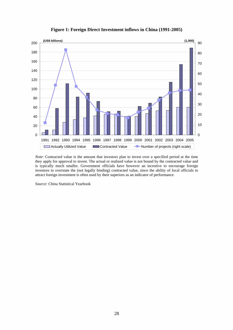
Figure 1: Foreign Direct Investment inflows in China (1991-2005)
0
20
40
60
80
100
120
140
160
180
200
1991 1992 1993 1994 1995 1996 1997 1998 1999 2000 2001 2002 2003 2004 2005
(US$ billions)
0
10
20
30
40
50
60
70
80
90(1,000)
Actually Utilized Value Contracted Value Number of projects (right scale) Note: Contracted value is the amount that investors plan to invest over a specified period at the time they apply for approval to invest. The actual or realized value is not bound by the contracted value and is typically much smaller. Government officials have however an incentive to encourage foreign investors to overstate the (not legally binding) contracted value, since the ability of local officials to attract foreign investment is often used by their superiors as an indicator of performance. Source: China Statistical Yearbook
28

Table 1: Summary statistics for manufacturing plants in China
Variable Domestic Foreign HMT Non-HMT JV WFOE Number of employees 968 876 924 756 793 959 Sales 32,840 47,142 36,224 50,081 49,358 44,282 Value added 4,901 7,266 5,805 7,759 7,815 6,411 Value added per worker 6.76 11.07 6.95 13.75 12.00 9.82 Capital per worker 16.98 20.80 13.95 25.91 24.64 16.83 Investment per worker 2.89 4.83 3.39 5.58 5.37 4.24 Labor productivity 47.30 80.78 50.38 98.24 88.88 72.28 Number of firms in 2002 7,232 5,553 2,915 2,315 2,915 2,620 in 2003 7,784 6,136 3,189 2,625 3,121 3,000 in 2004 8,463 6,903 3,573 3,012 3,400 3,491
Notes: - The summary statistics represent the mean over the period 2002-2004. - The number of employees is expressed in thousands of workers. - The remaining variables are expressed in thousands of US Dollars, using provincial price
indices to deflate. - The distinction between domestic and foreign plants is based on their legal form. - HMT: Hong Kong, Macau and Taiwan + tax paradises (Bermuda, Bahamas, Cayman Islands
and British Virgin Islands.)
Table 2: Summary statistics for exporting versus non-exporting plants
Variable Domestic Exporters
Domestic Non-exporters Exporters Non-exporters
Number of employees 1,402 769 1,185 784 Sales 50,286 24,875 55,169 34,051 Exports 11,379 0 24,349 0 Value added 7,551 3,623 8,151 5,209 Value added per worker 5.37 7.43 8.56 11.52 Capital per worker 11.17 19.63 16.15 29.38 Investment per worker 2.10 3.50 2.96 4.10 Labor productivity 39.86 50.70 65.21 79.18 Number of firms In 2002 3,126 4,106 7,388 5,397 In 2003 3,439 4,344 8,223 5,696 In 2004 795 807 2,113 1,146
Notes: - The group of domestic firms excludes Sino-foreign JVs. - The summary statistics represent the mean over the period 2002-2004. - The number of employees is expressed in thousands of workers. - The remaining variables are expressed in thousands of US Dollars, using provincial price
indices to deflate. - The distinction between domestic and foreign plants is based on their legal form.
29

Table 3: Sectoral spillovers in the Chinese manufacturing sector
TFP as dependent variable (1) (2) (3) (4) JV 0.166 0.180 0.175 0.173 (0.011)*** (0.012)*** (0.012)*** (0.012)*** Exporter - 0.092 0.087 0.087 (0.019)*** (0.019)*** (0.019)*** SEZ - - 0.089 0.047 (0.020)*** (0.014)*** Spillover 0.046 0.173 0.190 0.145 (0.025)* (0.030)*** (0.035)*** (0.032)*** Spillover x Exporter - -0.235 -0.224 -0.225 (0.039)*** (0.039)*** (0.039)*** Spillover x SEZ - - -0.058 - (0.040) Spillover x ETDZ - - - 0.064 (0.029)** Spillover x FTZ - - - -0.033 (0.030) Spillover x HIDZ - - - 0.033 (0.028) Spillover x BECZ - - - -0.160 (0.122) Spillover x EPZ - - - -0.035 (0.033) Observations 32,960 23,597 23,597 23,597 R-squared 0.499 0.515 0.517 0.518
Notes: The dependent variable is the logarithm of TFP estimated using the Olley-Pakes methodology. All regressions include 2-digit sector, province, and time dummies - Robust standard errors in parentheses - */**/*** significant at 10/5/1%.
30
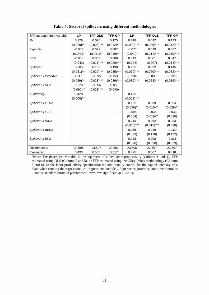
Table 4: Sectoral spillovers using different methodologies
TFP as dependent variable LP TFP-OLS TFP-OP LP TFP-OLS TFP-OP JV 0.226 0.095 0.175 0.218 0.092 0.173 (0.020)*** (0.006)*** (0.012)*** (0.020)*** (0.006)*** (0.012)*** Exporter -0.067 0.027 0.087 -0.073 0.029 0.087 (0.040)* (0.011)** (0.019)*** (0.040)* (0.011)*** (0.019)*** SEZ -0.008 0.053 0.089 0.013 0.001 0.047 (0.043) (0.011)*** (0.020)*** (0.024) (0.007) (0.014)*** Spillover 0.285 0.132 0.190 0.255 0.072 0.145 (0.081)*** (0.022)*** (0.035)*** (0.079)*** (0.020)*** (0.032)*** Spillover x Exporter -0.308 -0.095 -0.224 -0.294 -0.098 -0.225 (0.089)*** (0.023)*** (0.039)*** (0.089)*** (0.023)*** (0.039)*** Spillover x SEZ 0.228 -0.066 -0.058 - - - (0.090)** (0.023)*** (0.040) K_intensity 0.428 - - 0.425 - - (0.008)*** (0.008)*** Spillover x ETDZ - - - 0.132 0.039 0.064 (0.056)** (0.015)** (0.029)** Spillover x FTZ - - - -0.095 -0.036 -0.033 (0.064) (0.016)** (0.030) Spillover x HIDZ - - - 0.213 0.062 0.033 (0.055)*** (0.015)*** (0.028) Spillover x BECZ - - - 0.055 0.049 -0.160 (0.539) (0.128) (0.122) Spillover x EPZ - - - 0.062 0.008 -0.035 (0.070) (0.020) (0.033) Observations 23,595 23,597 23,597 23,595 23,597 23,597 R-squared 0.493 0.565 0.517 0.495 0.567 0.518
Notes: The dependent variable is the log form of either labor productivity (Column 1 and 4), TFP estimated using OLS (Column 2 and 5), or TFP estimated using the Olley-Pakes methodology (Column 3 and 6). In the labor-productivity specification we additionally control for the capital intensity of a plant when running the regressions. All regressions include 2-digit sector, province, and time dummies - Robust standard errors in parentheses - */**/*** significant at 10/5/1%.
31

Table 5: Spillovers and the role of ownership structure
TFP as dependent variable (1) (2) JV 0.162 0.169 (0.011)*** (0.012)*** Exporter - 0.077 (0.018)*** SEZ - 0.042 (0.016)** Spillover_JV 0.184 0.148 (0.030)*** (0.046)*** Spillover_WFOE -0.090 0.187 (0.042)** (0.074)** Spillover_JV x Exporter - -0.172 (0.054)*** Spillover_WFOE x Exporter - -0.250 (0.073)*** Spillover_JV x SEZ - 0.251 (0.053)*** Spillover_WFOE x SEZ - -0.243 (0.077)*** Observations 32,960 23,597 R-squared 0.500 0.519
Notes: The dependent variable is the logarithm of TFP estimated using the Olley-Pakes methodology. All regressions include 3-digit sector, city, and time dummies - Robust standard errors in parentheses - */**/*** significant at 10/5/1%.
Table 6: Spillovers according origin
TFP as dependent variable HMT (OP) Non-HMT (OP) JV 0.222 0.123 (0.015)*** (0.016)*** Region dummy -0.097 0.095 (0.021)*** (0.021)*** Exporter 0.063 0.026 (0.015)*** (0.014)* SEZ 0.075 0.082 (0.015)*** (0.015)*** Spillover 0.248 0.196 (0.060)*** (0.043)*** Spillover x Exporter -0.383 -0.154 (0.070)*** (0.043)*** Spillover x SEZ -0.067 -0.084 -0.070 (0.046)* Observations 23,789 23,678 R-squared 0.519 0.519
Notes: The dependent variable is the logarithm of TFP estimated using the Olley-Pakes methodology. All regressions include 3-digit sector, city, and time dummies - Robust standard errors in parentheses - */**/*** significant at 10/5/1%. HMT stands for Hong Kong, Macau and Taiwan + tax paradises (Bermuda, Bahamas, Cayman Islands and British Virgin Islands.)
32

Table 7: Robustness checks
TFP as dependent variable Original (OP) Employment (a) Regional (b) HHI (c) DL JV 0.175 0.176 0.167 0.175 0.077 (0.012)*** (0.012)*** (0.012)*** (0.012)*** (0.012)*** Exporter 0.087 0.094 0.056 0.088 -0.007 (0.019)*** (0.017)*** (0.011)*** (0.019)*** (0.017) SEZ 0.089 0.104 0.058 0.089 0.042 (0.020)*** (0.017)*** (0.018)*** (0.020)*** (0.018)** HHI3 - - - 0.351 - (0.084)*** Spillover 0.190 0.277 0.166 0.246 0.070 (0.035)*** (0.046)*** (0.025)*** (0.039)*** (0.033)** Spillover x Exporter -0.224 -0.299 -0.171 -0.230 -0.042 (0.039)*** (0.046)*** (0.026)*** (0.039)*** (0.038) Spillover x SEZ -0.058 -0.110 -0.015 -0.058 0.024 (0.040) (0.046)** (0.036) (0.040) (0.040) Spillover x HHI3 - - - -0.568 - (0.160)*** Observations 23,597 23,597 23,597 23,597 23,597 R-squared 0.517 0.519 0.518 0.518 0.439 Notes: The dependent variable is the logarithm of TFP estimated using the Olley-Pakes methodology (except in last column -DL- where TFP is estimated using the De Loecker methodology). All regressions include 3-digit sector, city, and time dummies - Robust standard errors in parentheses - */**/*** significant at 10/5/1%. (a) Employment spillovers are measured by the share of foreign employment in total employment at the 3-digit US SIC87 level. (b) Regional spillovers are defined as the share of foreign sales in total sales at the city level. (c) The Herfindahl-Hirschman Index is calculated at the 3-digit US SIC87 level.
33

Table 8: Herfindahl-Hirschman Index
USSIC Description HHI 20 Food and kindred products 0.03 21 Tobacco products 0.33 22 Textile mill products 0.03 23 Apparel and other textile products 0.03 24 Lumber and wood products 0.11 25 Furniture and fixtures 0.06 26 Paper and allied products 0.06 27 Printing and publishing 0.12 28 Chemicals and allied products 0.02 29 Petroleum and coal products 0.10 30 Rubber and miscellaneous plastics products 0.03 31 Leather and leather products 0.04 32 Stone, clay, and glass products 0.04 33 Primary metal industries 0.03 34 Fabricated metal products 0.05 35 Industrial machinery and equipment 0.04 36 Electronic and other electric equipment 0.03 37 Transportation equipment 0.06 38 Instruments and related products 0.07 39 Miscellaneous manufacturing industries 0.05
Note: The HHI index is calculated at the 3-digit US SIC87 level. The indices represent the mean competition degree within a sector over the three years of our dataset.
34

35
Appendix B: Regional Distribution of FDI in China

Number of firms Distribution of foreign firms across sectors US SIC Description
Total JV WFOE HMT Non-HMT
Foreign share in
total sales20 Food and kindred products 1,175 300 154 6.46% 8.56% 46.33%21 Tobacco products 27 3 1 0.06% 0.04% 6.59%22 Textile mill products 1,370 259 188 9.13% 5.44% 30.46%23 Apparel and other textile products 1,128 334 310 11.01% 10.14% 52.54%24 Lumber and wood products 124 31 17 0.78% 0.77% 30.43%25 Furniture and fixtures 183 46 67 2.26% 1.40% 70.17%26 Paper and allied products 358 81 46 2.23% 1.90% 48.69%27 Printing and publishing 119 39 20 1.44% 0.49% 55.99%28 Chemicals and allied products 1,319 252 128 5.05% 7.34% 36.34%29 Petroleum and coal products 128 17 11 0.25% 0.70% 24.81%30 Rubber and miscellaneous plastics products 655 156 234 7.59% 4.84% 60.90%31 Leather and leather products 514 122 198 5.83% 4.49% 60.64%32 Stone, clay, and glass products 857 140 56 3.20% 3.26% 28.40%33 Primary metal industries 834 125 63 2.98% 3.05% 23.66%34 Fabricated metal products 539 117 120 4.11% 3.62% 46.83%35 Industrial machinery and equipment 1,128 197 261 6.05% 8.99% 54.74%36 Electronic and other electric equipment 1,930 537 672 18.16% 21.55% 67.05%37 Transportation equipment 691 164 100 2.76% 5.97% 55.28%38 Instruments and related products 257 59 91 2.16% 2.77% 63.06%39 Miscellaneous manufacturing industries 584 142 263 8.50% 4.67% 67.90% Total 13,920 3,121 3,000 100.00% 100.00% 48.32%
36
Appendix C: Sectoral distribution of FDI in China
Notes: - The distinction between domestic and Sino-foreign Joint-Ventures (JV) and Wholly Foreign Owned Enterprises (WFOE) respectively is
based on their legal form, - HMT: Hong Kong, Macau and Taiwan + tax paradises (Bermuda, Bahamas, Cayman Islands and British Virgin Islands).

Appendix F.1: Estimates of production function – Domestic plants
OLS OP DL mean s.e. mean s.e. mean s.e. Food and kindred products Labor 0.090 0.011 0.082 0.015 0.082 0.015 Materials 0.842 0.011 0.831 0.016 0.829 0.018 Capital 0.055 0.006 0.059 0.015 0.058 0.013 Tobacco products Labor 0.041 0.044 0.073 0.042 0.058 0.069 Materials 0.810 0.027 0.771 0.023 0.770 0.022 Capital 0.072 0.039 0.044 0.089 0.037 0.085 Textile mill products Labor 0.073 0.009 0.066 0.013 0.074 0.015 Materials 0.878 0.014 0.863 0.022 0.877 0.025 Capital 0.030 0.006 0.052 0.014 0.053 0.013 Apparel and other textile products Labor 0.128 0.012 0.096 0.012 0.096 0.013 Materials 0.844 0.011 0.859 0.012 0.859 0.013 Capital 0.037 0.007 0.035 0.012 0.034 0.011 Lumber and wood products Labor 0.057 0.017 0.025 0.025 0.021 0.025 Materials 0.902 0.011 0.909 0.017 0.914 0.018 Capital 0.038 0.007 0.052 0.019 0.021 0.018 Furniture and fixtures Labor 0.110 0.023 0.117 0.029 0.117 0.029 Materials 0.855 0.016 0.833 0.020 0.833 0.021 Capital 0.017 0.013 0.040 0.017 0.040 0.017 Paper and allied products Labor 0.113 0.032 0.059 0.025 0.081 0.028 Materials 0.825 0.050 0.800 0.051 0.822 0.057 Capital 0.040 0.014 0.100 0.013 0.112 0.012 Printing and publishing Labor 0.045 0.028 0.028 0.038 -0.002 0.036 Materials 0.825 0.022 0.858 0.027 0.861 0.026 Capital 0.040 0.024 0.109 0.030 0.100 0.031 Chemicals and allied products Labor 0.079 0.013 0.066 0.017 0.072 0.017 Materials 0.740 0.018 0.706 0.026 0.715 0.028 Capital 0.107 0.012 0.080 0.031 0.083 0.032 Petroleum and coal products Labor 0.084 0.042 0.122 0.046 0.123 0.045 Materials 0.844 0.034 0.824 0.035 0.811 0.039 Capital 0.063 0.044 0.018 0.038 0.026 0.043 Rubber and miscellaneous plastics products Labor 0.081 0.014 0.046 0.016 0.048 0.017 Materials 0.866 0.019 0.886 0.015 0.884 0.016 Capital 0.029 0.010 0.046 0.015 0.047 0.014 Leather and leather products Labor 0.155 0.022 0.124 0.026 0.127 0.025 Materials 0.804 0.024 0.822 0.046 0.864 0.046 Capital 0.048 0.012 0.072 0.021 0.075 0.024
37

Appendix F.1 continue
OLS OP DL mean s.e. mean s.e. mean s.e. Stone, clay, and glass products Labor 0.137 0.017 0.103 0.013 0.101 0.013 Materials 0.850 0.011 0.861 0.008 0.866 0.010 Capital 0.030 0.013 0.044 0.018 0.044 0.018 Primary metal industries Labor 0.063 0.006 0.058 0.008 0.061 0.008 Materials 0.906 0.007 0.887 0.011 0.894 0.011 Capital 0.030 0.005 0.030 0.010 0.031 0.009 Fabricated metal products Labor 0.096 0.014 0.099 0.019 0.099 0.019 Materials 0.844 0.014 0.821 0.016 0.821 0.016 Capital 0.050 0.009 0.049 0.023 0.053 0.021 Industrial machinery and equipment Labor 0.093 0.012 0.098 0.014 0.098 0.014 Materials 0.818 0.013 0.803 0.019 0.804 0.019 Capital 0.061 0.008 0.060 0.015 0.060 0.016 Electronic and other electric equipment Labor 0.109 0.020 0.096 0.022 0.096 0.022 Materials 0.802 0.017 0.805 0.019 0.805 0.020 Capital 0.081 0.013 0.089 0.015 0.088 0.016 Transportation equipment Labor 0.109 0.014 0.081 0.011 0.083 0.012 Materials 0.850 0.013 0.844 0.015 0.843 0.015 Capital 0.037 0.008 0.033 0.018 0.032 0.018 Instruments and related products Labor 0.052 0.024 0.007 0.037 0.004 0.037 Materials 0.804 0.030 0.776 0.045 0.793 0.050 Capital 0.085 0.021 0.021 0.069 0.021 0.062 Miscellaneous manufacturing industries Labor 0.120 0.021 0.105 0.023 0.105 0.023 Materials 0.816 0.022 0.812 0.024 0.813 0.025 Capital 0.065 0.014 0.109 0.020 0.110 0.021
Note: To allow the factor proportions and the economies of scale varying across the different sectors, the production function is estimated for each of the twenty US SIC 2-digit sectors separately. For sector “Tobacco products” we do not have enough observations to estimate the production for domestic versus joint-ventures separately. The coefficients are estimates for both groups jointly.
38

Appendix F.2: Estimates of production function – Sino-foreign joint-ventures
OLS OP DL mean s.e. mean s.e. mean s.e. Food and kindred products Labor 0.064 0.018 0.031 0.019 0.032 0.019 Materials 0.839 0.015 0.830 0.016 0.829 0.016 Capital 0.099 0.016 0.012 0.037 0.011 0.040 Tobacco products Labor 0.041 0.044 0.073 0.042 0.058 0.069 Materials 0.810 0.027 0.771 0.023 0.770 0.022 Capital 0.072 0.039 0.044 0.089 0.037 0.085 Textile mill products Labor 0.073 0.012 0.062 0.014 0.062 0.014 Materials 0.880 0.014 0.877 0.019 0.877 0.020 Capital 0.020 0.008 0.038 0.022 0.038 0.022 Apparel and other textile products Labor 0.176 0.022 0.148 0.022 0.149 0.023 Materials 0.759 0.019 0.772 0.021 0.771 0.021 Capital 0.060 0.012 0.053 0.025 0.055 0.026 Lumber and wood products Labor 0.000 0.000 0.000 0.000 0.000 0.000 Materials 0.000 0.000 0.000 0.000 0.000 0.000 Capital 0.000 0.000 0.000 0.000 0.000 0.000 Furniture and fixtures Labor 0.086 0.024 0.054 0.017 0.053 0.015 Materials 0.869 0.024 0.879 0.022 0.876 0.023 Capital 0.044 0.016 0.049 0.031 0.055 0.032 Paper and allied products Labor 0.036 0.037 0.020 0.026 0.022 0.028 Materials 0.901 0.037 0.916 0.040 0.918 0.039 Capital 0.021 0.023 0.131 0.048 0.131 0.046 Printing and publishing Labor 0.042 0.025 0.058 0.045 0.084 0.039 Materials 0.901 0.024 0.914 0.039 0.927 0.037 Capital 0.021 0.023 -0.005 0.071 0.002 0.052 Chemicals and allied products Labor 0.151 0.029 0.157 0.039 0.157 0.039 Materials 0.664 0.035 0.657 0.044 0.654 0.047 Capital 0.138 0.020 0.091 0.046 0.083 0.048 Petroleum and coal products Labor 0.037 0.025 0.011 0.037 0.016 0.033 Materials 0.851 0.032 0.820 0.055 0.847 0.063 Capital 0.028 0.023 0.055 0.050 0.035 0.038 Rubber and miscellaneous plastics products Labor 0.068 0.013 0.048 0.011 0.049 0.011 Materials 0.861 0.019 0.885 0.016 0.885 0.016 Capital 0.051 0.010 0.058 0.018 0.058 0.020 Leather and leather products Labor 0.201 0.045 0.112 0.025 0.114 0.024 Materials 0.704 0.054 0.832 0.034 0.877 0.034 Capital 0.070 0.032 0.066 0.093 0.072 0.097
39

40
Appendix F.2 continue
OLS OP DL mean s.e. mean s.e. mean s.e. Stone, clay, and glass products Labor 0.037 0.021 0.060 0.024 0.064 0.026 Materials 0.848 0.043 0.801 0.095 0.791 0.101 Capital 0.061 0.019 0.084 0.039 0.072 0.048 Primary metal industries Labor 0.049 0.009 0.056 0.012 0.069 0.013 Materials 0.903 0.014 0.892 0.013 0.912 0.013 Capital 0.061 0.009 0.051 0.016 0.046 0.011 Fabricated metal products Labor 0.023 0.012 0.026 0.017 0.025 0.017 Materials 0.906 0.016 0.888 0.021 0.887 0.022 Capital 0.051 0.012 0.075 0.035 0.076 0.031 Industrial machinery and equipment Labor 0.094 0.046 0.029 0.015 0.032 0.015 Materials 0.843 0.036 0.884 0.014 0.886 0.014 Capital 0.024 0.025 0.052 0.010 0.050 0.011 Electronic and other electric equipment Labor 0.060 0.017 0.043 0.022 0.044 0.021 Materials 0.856 0.028 0.876 0.030 0.876 0.030 Capital 0.046 0.011 -0.019 0.037 0.024 0.035 Transportation equipment Labor 0.030 0.018 0.006 0.016 0.004 0.017 Materials 0.918 0.017 0.914 0.018 0.912 0.018 Capital 0.051 0.012 0.022 0.026 0.027 0.025 Instruments and related products Labor 0.000 0.022 -0.015 0.027 -0.015 0.029 Materials 0.825 0.054 0.917 0.047 0.917 0.047 Capital 0.083 0.032 -0.024 0.118 -0.026 0.114 Miscellaneous manufacturing industries Labor 0.166 0.024 0.176 0.035 0.170 0.035 Materials 0.773 0.031 0.738 0.063 0.735 0.064 Capital 0.062 0.015 0.109 0.030 0.112 0.032
Note: To allow the factor proportions and the economies of scale varying across the different sectors, the production function is estimated for each of the twenty US SIC 2-digit sectors separately. For sector “Tobacco products” we do not have enough observations to estimate the production for domestic versus joint-ventures separately. The coefficients are estimates for both groups jointly.

Appendix F.3: Estimated output coefficients (βq) across sectors, using De Loecker (2007)
Domestic JV USSIC Description
beta_q s.e. t-stat markup beta_q s.e. t-stat markup 20 Food and kindred products 0.009 0.011 0.81 1.01 0.010 0.019 0.54 1.01 21 Tobacco products 0.030 0.087 0.35 1.03 0.030 0.087 0.35 1.03 22 Textile mill products 0.025 0.013 1.94 1.03 -0.001 0.012 -0.05 1.00 23 Apparel and other textile products -0.003 0.012 -0.21 1.00 0.014 0.021 0.68 1.01 24 Lumber and wood products -0.011 0.014 -0.75 0.99 0.147 0.217 0.68 1.17 25 Furniture and fixtures -0.002 0.020 -0.12 1.00 0.015 0.020 0.74 1.02 26 Paper and allied products 0.060 0.023 2.55 1.06 -0.015 0.018 -0.83 0.99 27 Printing and publishing -0.054 0.025 -2.15 0.95 -0.064 0.024 -2.63 0.94 28 Chemicals and allied products 0.029 0.012 2.35 1.03 0.013 0.033 0.40 1.01 29 Petroleum and coal products 0.039 0.031 1.26 1.04 -0.048 0.091 -0.53 0.95 30 Rubber and miscellaneous plastics products 0.010 0.014 0.73 1.01 0.005 0.013 0.40 1.01 31 Leather and leather products 0.049 0.024 2.06 1.05 0.052 0.027 1.94 1.05 32 Stone, clay, and glass products -0.011 0.007 -1.48 0.99 0.024 0.026 0.94 1.02 33 Primary metal industries 0.013 0.006 2.17 1.01 0.034 0.012 2.88 1.04 34 Fabricated metal products -0.003 0.012 -0.22 1.00 0.007 0.015 0.45 1.01 35 Industrial machinery and equipment 0.000 0.009 -0.02 1.00 -0.025 0.014 -1.84 0.98 36 Electronic and other electric equipment 0.001 0.014 0.07 1.00 -0.005 0.013 -0.43 0.99 37 Transportation equipment 0.005 0.008 0.63 1.01 0.012 0.014 0.89 1.01 38 Instruments and related products -0.054 0.031 -1.72 0.95 -0.003 0.041 -0.07 1.00 39 Miscellaneous manufacturing industries -0.009 0.018 -0.50 0.99 0.027 0.028 0.96 1.03 Note: The coefficients represent the means and standard deviations of the estimated demand variation in sector j. The absolute values of the means are a measure for the sectoral Lerner indices.
41

OLS OP DL Mean Standard deviation Mean Standard deviation Mean Standard deviation ussic2
D JV D-JV D JV D-JV D JV D-JV D JV D-JV D JV D-JV D JV D-JV 20 0.77 0.67 0.09 0.25 0.28 -0.03 0.89 1.74 -0.86 0.25 0.31 -0.06 0.91 1.75 -0.84 0.00 0.31 -0.31 21 1.38 1.64 -0.25 0.23 0.50 -0.27 1.79 2.05 -0.26 0.24 0.49 -0.25 1.96 2.21 -0.25 0.25 0.48 -0.23 22 0.61 0.71 -0.10 0.15 0.14 0.01 0.61 0.67 -0.05 0.15 0.14 0.01 0.36 0.67 -0.31 0.24 0.14 0.10 23 0.55 0.87 -0.31 0.17 0.23 -0.06 0.64 0.98 -0.34 0.17 0.23 -0.06 0.65 0.98 -0.33 0.16 0.23 -0.07 24 0.45 0.58 -0.13 0.10 0.11 -0.01 0.49 0.12 0.37 0.10 0.13 -0.03 0.70 0.09 0.61 0.17 0.13 0.04 25 0.73 0.58 0.16 0.14 0.16 -0.02 0.71 0.65 0.06 0.14 0.16 -0.02 0.71 0.64 0.07 0.11 0.16 -0.05 26 0.80 0.85 -0.05 0.23 0.21 0.03 0.87 -0.22 1.09 0.24 0.29 -0.05 0.30 -0.25 0.55 0.14 0.30 -0.16 27 0.81 0.07 0.74 0.17 0.13 0.04 0.51 0.81 -0.30 0.18 0.16 0.02 0.74 0.46 0.28 0.25 0.15 0.10 28 1.39 1.65 -0.25 0.34 0.40 -0.06 2.04 2.10 -0.07 0.35 0.41 -0.06 1.84 2.20 -0.36 0.18 0.41 -0.23 29 0.74 1.42 -0.68 0.30 0.17 0.13 1.12 1.63 -0.52 0.31 0.17 0.14 1.17 1.50 -0.33 0.36 0.17 0.19 30 0.74 0.72 0.02 0.21 0.15 0.05 0.65 0.57 0.08 0.21 0.16 0.05 0.66 0.57 0.09 0.31 0.16 0.15 31 0.68 1.11 -0.43 0.20 0.28 -0.08 0.55 0.61 -0.06 0.21 0.33 -0.12 0.01 0.00 0.00 0.21 0.34 -0.13 32 0.52 0.98 -0.46 0.19 0.26 -0.07 0.52 1.07 -0.55 0.20 0.26 -0.07 0.50 1.24 -0.74 0.22 0.27 -0.05 33 0.53 0.60 -0.07 0.15 0.13 0.02 0.68 0.50 0.18 0.15 0.13 0.02 0.57 0.22 0.35 0.20 0.13 0.06 34 0.70 0.59 0.11 0.17 0.14 0.03 0.90 0.55 0.35 0.17 0.14 0.03 0.87 0.55 0.32 0.15 0.14 0.01 35 0.92 1.13 -0.21 0.22 0.30 -0.08 1.03 0.88 0.15 0.22 0.31 -0.10 1.03 0.87 0.16 0.17 0.31 -0.14 36 0.85 0.96 -0.11 0.27 0.31 -0.03 0.84 1.42 -0.58 0.27 0.32 -0.05 0.84 1.04 -0.20 0.22 0.31 -0.09 37 0.66 0.47 0.19 0.19 0.18 0.00 0.94 0.94 0.00 0.19 0.19 -0.01 0.94 0.92 0.02 0.27 0.19 0.08 38 1.16 1.40 -0.24 0.23 0.34 -0.11 2.18 1.48 0.70 0.27 0.37 -0.10 2.06 1.50 0.56 0.19 0.37 -0.18 39 0.69 0.81 -0.13 0.20 0.25 -0.05 0.52 0.72 -0.20 0.21 0.25 -0.05 0.50 0.75 -0.25 0.26 0.26 0.01
42
Appendix F.4: Estimated Total Factor Productivity
Note: TFP is calculated as a residual: , where (with h = l, m, k) stands for the estimators of the respective inputs using the different approaches discussed in Chapter 5.
itkitmitlitit kmlyTFP βββ ˆˆˆln −−−= hβ̂

Appendix F.5: Kernel density functions of TFP
Domestic plants
01
23
-1 -.5 0 .5 1TFP
TFP_OLS TFP_OPTFP_DL
Panel b: Sector 28 - Chemicals and allied products
01
23
4
-.5 0 .5 1TFP
TFP_OLS TFP_OPTFP_DL
Panel a: Sector 23 - Apparel and other textile products
Sino-foreign joint-ventures
43
0.5
11.
52
2.5
-1 -.5 0 .5 1TFP
TFP_OLS TFP_OPTFP_DL
Panel c: Sector 23 - Apparel and other textile products
01
23
4
-1 -.5 0 .5 1TFP
TFP_OLS TFP_OPTFP_DL
Panel d: Sector 33 - Primary metal industries
Note: The graphs represent the kernel density functions of the standardized TFP-levels for domestic plants versus Sino-foreign joint-ventures. We subtract the sector mean to standardize the TFP-levels around zero, and use cut-off levels at -1 and 1. This improves the visibility of the comparison between methodologies. The density functions are based on 484 domestic plants and 334 JVs in sector 23 - 939 domestic plants in sector 28 - 125 JVs in sector 33.


