RESEARCH PAPER
FRACTIONAL BOUNDARY VALUE PROBLEMS:
ANALYSIS AND NUMERICAL METHODS
Neville J. Ford 1, M. Luısa Morgado 2
Abstract
In this paper we consider nonlinear boundary value problems for differ-ential equations of fractional order α, 0 < α < 1. We study the existenceand uniqueness of the solution and extend existing published results. In thelast part of the paper we study a class of prototype methods to determinetheir numerical solution.
MSC 2010 : Primary 65L05; Secondary 34A08, 26A33Key Words and Phrases: fractional calculus, fractional ordinary differ-
ential equations, Caputo derivative, numerical methods
1. Introduction
In this paper we focus on boundary value problems for fractional orderdifferential equations of the form
Dα∗ y(t) = f(t, y(t)), t ∈ [0, T ] (1.1)y(a) = ya, (1.2)
where 0 < a < T , f is a suitably behaved function and Dα∗ denotes theCaputo differential operator of order α /∈ N ([1]).
The Caputo differential operator can be defined by
Dα∗ y(t) := Dα(y − T [y])(t),
c© 2011 Diogenes Co., Sofiapp. 554–567 , DOI: 10.2478/s13540-011-0034-4
FRACTIONAL BOUNDARY VALUE PROBLEMS 555
where T [y] is the Taylor polynomial of degree �α� for y, centered at 0,and Dα is the Riemann-Liouville derivative of order α ([9]). The latter isdefined by Dα := D�α�J�α�−α, with Jβ representing the Riemann-Liouvilleintegral operator
Jβy(t) :=1
Γ(β)
∫ t
0(t − s)β−1y(s)ds
and D�α� as the classical integer order derivative. Here, �α� denotes thebiggest integer smaller than α, and �α� represents the smallest integergreater than or equal to α.
In [5], Diethelm and Ford studied problem (1.1)-(1.2) in the case wherea = 0, that is they considered an initial value problem and they analyzednot only the issues of existence and uniqueness of the solution, but also thedependence of the solution on the parameters in the differential equation.
Since the case where the conditions are given at a = 0 is well-understood,here we consider the boundary value problem where a �= 0 and we seek so-lutions over a finite interval [0, T ] where 0 < a < T .
Concerning the case where a > 0, Diethelm and Ford recently investi-gated the uniqueness of the solution. They proved that, under some simplenatural conditions on f , there is at most one initial value y0 for which thesolution of the problem
Dα∗ y(t) = f(t, y(t)), t ∈ [0, T ] (1.3)y(0) = y0, (1.4)
satisfies y(a) = ya. The fundamental theorem asserting that the problemunder consideration is well-posed is the following:
Theorem 1.1 ([4]). Let 0 < α < 1 and assume f : [0, b]× [c, d] → R tobe continuous and satisfy a Lipschitz condition with respect to the secondvariable. Consider two solutions y1 and y2 to the differential equation
Dα∗0yj(t) = f(t, yj(t)) (j = 1, 2) (1.5)
subject to the initial conditions yj(0) = yj0, respectively, where y10 �= y20.Then, for all t where both y1(t) and y2(t) exist, we have y1(t) �= y2(t).
In other words, if we know the value of a solution y to the equation(1.1) at t = a, then there is at most one corresponding value of y(s) at anys ∈ [0, a].
But in that paper, the authors did not provide results on the existenceof solutions and, to our knowledge, there is still no complete proof of the
556 N.J. Ford, M.L. Morgado
existence of the solution of problem (1.1)-(1.2) in the literature. This willbe one of our main goals in this paper.
The paper is organized as follows: In Section 2 we discuss the existenceand uniqueness of solutions to the FBVP (1.1)-(1.2).
The authors of [4] also proposed a numerical scheme for the solutionof FBVPs. Such scheme, based on a shooting algorithm to find the appro-priate initial value corresponding to a particular boundary value, providesa useful prototype approach. In Section 3 we investigate more fully thistype of approach when a range of basic numerical schemes are utilized. Wealso compare the efficiency of the numerical methods by considering theirperformance on problems with non-smooth solutions.
Finally, in the last Section 4 we present some conclusions and somesuggestions for future work.
2. Existence and uniqueness of the solution
In this section our main aim is to establish a new basic existence the-orem for the boundary value problem (1.1)-(1.2). This will combine withexisting known results to provide a comprehensive existence and uniquenesstheory.
First we recall a well known result from fractional calculus:
Lemma 2.1. If the function f is continuous, the initial value problem(1.3)-(1.4) is equivalent to the following Volterra integral equation of thesecond kind:
y(t) = y0 +1
Γ(α)
∫ t
0(t − s)α−1f(s, y(s))ds. (2.6)
Assume a > 0 is fixed, y(a) = ya and 0 ≤ t ≤ a, we have, taking (2.6)into account
y(t) = y0 +1
Γ(α)
∫ t
0(t − s)α−1f(s, y(s))ds
= y(a) − 1Γ(α)
∫ a
0(a − s)α−1f(s, y(s))ds
+1
Γ(α)
∫ t
0(t − s)α−1f(s, y(s))ds . (2.7)
It follows that any solution of (2.7) for t ∈ [0, a] also satisfies (1.1)-(1.2).We use this observation as the motivation for the following theorem:
FRACTIONAL BOUNDARY VALUE PROBLEMS 557
Theorem 2.1. Let a > 0 and ya be constant, 0 < α < 1. For theequation
y(t) = ya +1
Γ(α)
∫ t
0(t− s)α−1f(s, y(s))ds− 1
Γ(α)
∫ a
0(a− s)α−1f(s, y(s))ds
(2.8)we assume the following conditions hold:
(1) f satisfies a Lipschitz condition with Lipschitz constant L > 0 withrespect to its second argument,
(2)2Laα
Γ(α + 1)< 1.
Then (2.8) has a unique solution y(t) for 0 ≤ t ≤ a.
P r o o f. We rewrite (2.8) as the Fredholm equation:
y(t) = ya +1
Γ(α)
∫ a
0(t − s)α−1Ξ[0,t](s)f(s, y(s))ds
− 1Γ(α)
∫ a
0(a − s)α−1f(s, y(s))ds, (2.9)
where Ξ is the indicator function of the interval [0, t].As usual, we set up the recurrence
y0(t) = ya,
yn(t) = ya +1
Γ(α)
∫ a
0(t − s)α−1Ξ[0,t](s)f(s, yn−1(s))ds
− 1Γ(α)
∫ a
0(a − s)α−1f(s, yn−1(s))ds.
It follows that
‖yn+1 − yn‖≤ 1
Γ(α)L‖yn−yn−1‖
(|∫ t
0(t−s)α−1−(a−s)α−1ds| + |
∫ a
t(a−s)α−1ds|
)
=1
Γ(α)‖yn − yn−1‖L
α(|0 − tα − (a − t)α + aα| + |0 − (a − t)α|)
≤ 2Laα
Γ(α + 1)‖yn − yn−1‖
for t ∈ [0, a], and so the sequence {yn} converges absolutely and uniformlyto a solution of (2.9) and hence of (2.8).
The uniqueness also follows in the usual way. �
As a consequence of Theorem 2.1, we find that, subject to the condi-tions of the theorem, every FBVP (1.1)-(1.2) coincides with a unique initial
558 N.J. Ford, M.L. Morgado
condition y0. It follows that there is an exact correspondence between frac-tional boundary value problems and initial value problems. In other words,we may conclude the following:
Lemma 2.2. If the function f is continuous and satisfies a Lipschitzcondition with Lipschitz constant L > 0 with respect to its second argu-ment, and if 2Laα
Γ(α+1) < 1, then the boundary value problem (1.1)-(1.2) is
equivalent to the integral equation (2.7).
The existence and uniqueness theory for the FBVP for t > a is inheritedfrom the corresponding initial value problem theory. For details, see [5].
3. Numerical methods and results
If f is continuous and satisfies a Lipschitz condition with respect tothe second variable, from the results in [4] we know that for the solutionof (1.1) that passes through the point (a, ya), we are able to find at mostone point (0, y0) that also lies on the same solution trajectory. Accordingto Theorem 2.1 we now know that if, in addition, 2Laα
Γ(α+1) < 1 then sucha point (0, y0) will in fact exist. In the paper [4] the solution was foundby using a shooting algorithm based on the bisection method. In whatfollows we will use a different approach where the bisection is replaced bythe secant method. Also other numerical methods for solving the initialvalue problems than the one used by the authors of that paper, will beconsidered.
To be more precise, our first step will be to find two initial guesses fory(0), say y01 and y02, satisfying y(a)|y(0)=y01
< w < y(a)|y(0)=y02. Next,
iterate by the secant method to provide successive approximations for y0
until the distance between the two last approximations does not exceed agiven tolerance ε. In our numerical experiments we have used ε = 10−8.
Note that the evaluation of y(a) may require the use of a IVP numericalsolver. The methods that we used to solve the initial value problem
Dα∗ (y(t)) = f(t, y(t)), (3.10)
y(0) = y0, (3.11)
are listed bellow:
Method 1: The first method we have considered was the fractionalAdams scheme of [6], the one also used in [4];
Method 2: This is a finite difference method based on the definitionof the Grunwald-Letnikov operator (see, for example, [7]);
FRACTIONAL BOUNDARY VALUE PROBLEMS 559
Method 3: Fractional backward difference based on quadrature (see,for example, [2], [7]);
Method 4: A higher order method proposed initially by Lubich withconvergence order p = 3 ([3], [8]).
In order to compare the efficiency of these methods, let us begin withthe following example:
Dα∗ (y(t)) = −1
2y(t) +
12t2 + 2
t2−α
Γ(3 − α), 0 < t ≤ 1, (3.12)
y(0.5) = 0.25,
whose analytical solution is known and is given by y(t) = t2.Since in our numerical methods we begin by determining the value of
y(0) for which the solution of the initial value problem matches the givenboundary condition, it is natural, in order to test its accuracy, to evaluatethe absolute error at the point where that boundary condition is imposed(generally we do not have an analytical solution to compare the obtainednumerical results). For this example, with α = 1
4 , the absolute errors att = 0.5 and t = 1 and the obtained values of y(0) are presented in Tables1, 2, 3 and 4.
h y(0) Absolute error at t = 0.5 Absolute error at t = 11/10 −2.60518 × 10⁻² < 10−25 1.57 × 10⁻²
1/20 −1.01031 × 10⁻² < 10−25 5.97 × 10⁻³
1/40 −3.91042 × 10⁻³ < 10−25 2.32 × 10⁻³
1/80 −1.52436 × 10⁻³ < 10−25 9.12 × 10⁻⁴
1/160 −5.99889 × 10⁻⁴ < 10−25 3.63 × 10⁻⁴
1/320 −2.38312 × 10⁻⁴ < 10−25 1.46 × 10⁻⁴
Table 1. Comparison with the exact solution(shooting algorithm with Method 1 to solve the IVP)
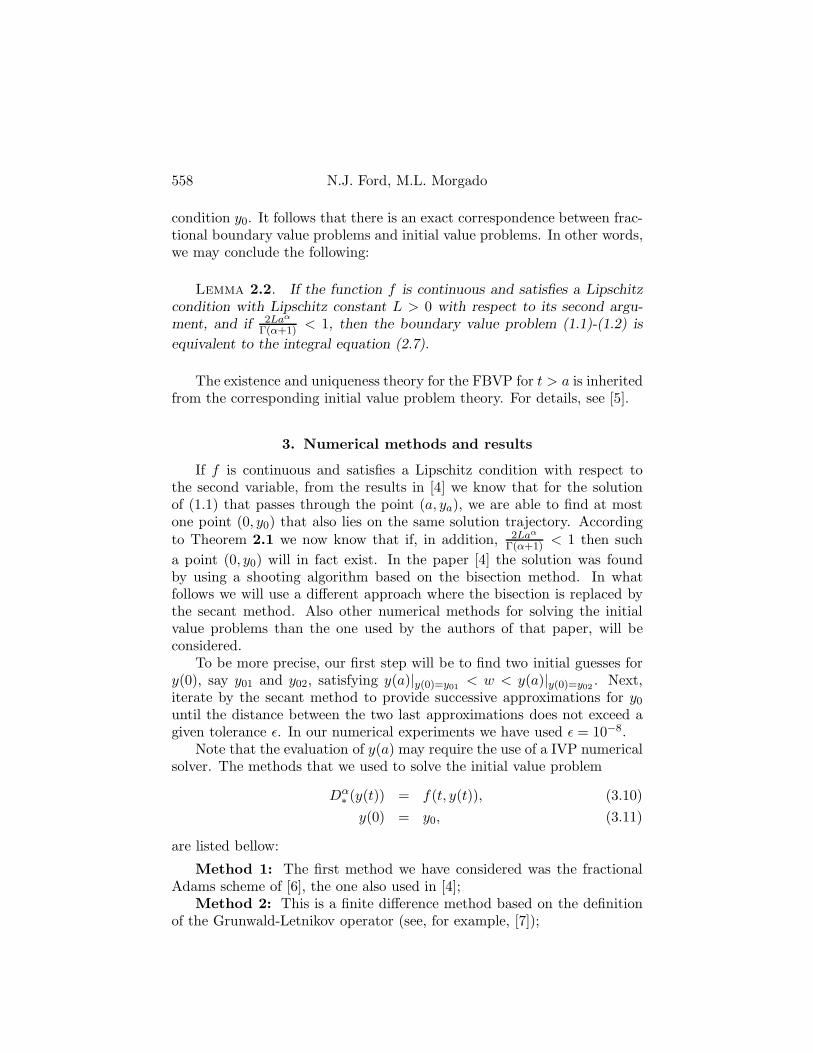
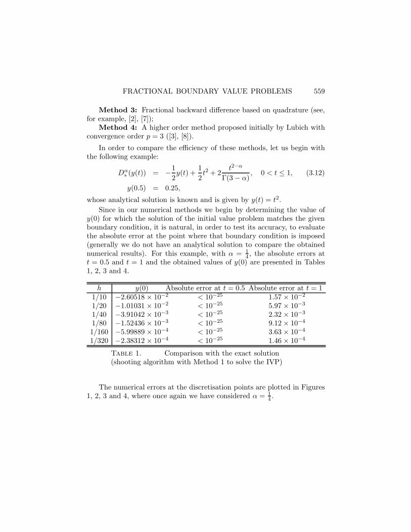
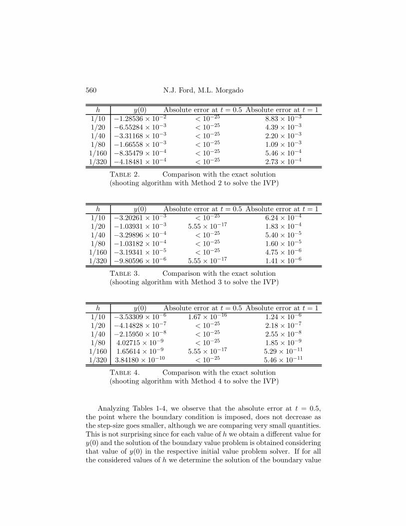
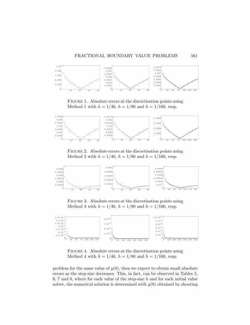
The numerical errors at the discretisation points are plotted in Figures1, 2, 3 and 4, where once again we have considered α = 1
4 .
560 N.J. Ford, M.L. Morgado
h y(0) Absolute error at t = 0.5 Absolute error at t = 11/10 −1.28536 × 10⁻² < 10−25 8.83 × 10⁻³
1/20 −6.55284 × 10⁻³ < 10−25 4.39 × 10⁻³
1/40 −3.31168 × 10⁻³ < 10−25 2.20 × 10⁻³
1/80 −1.66558 × 10⁻³ < 10−25 1.09 × 10⁻³
1/160 −8.35479 × 10⁻⁴ < 10−25 5.46 × 10⁻⁴
1/320 −4.18481 × 10⁻⁴ < 10−25 2.73 × 10⁻⁴
Table 2. Comparison with the exact solution(shooting algorithm with Method 2 to solve the IVP)
h y(0) Absolute error at t = 0.5 Absolute error at t = 11/10 −3.20261 × 10⁻³ < 10−25 6.24 × 10⁻⁴
1/20 −1.03931 × 10⁻³ 5.55 × 10⁻¹⁷ 1.83 × 10⁻⁴
1/40 −3.29896 × 10⁻⁴ < 10−25 5.40 × 10⁻⁵
1/80 −1.03182 × 10⁻⁴ < 10−25 1.60 × 10⁻⁵
1/160 −3.19341 × 10⁻⁵ < 10−25 4.75 × 10⁻⁶
1/320 −9.80596 × 10⁻⁶ 5.55 × 10⁻¹⁷ 1.41 × 10⁻⁶
Table 3. Comparison with the exact solution(shooting algorithm with Method 3 to solve the IVP)
h y(0) Absolute error at t = 0.5 Absolute error at t = 11/10 −3.53309 × 10⁻⁶ 1.67 × 10⁻¹⁶ 1.24 × 10⁻⁶
1/20 −4.14828 × 10⁻⁷ < 10−25 2.18 × 10⁻⁷
1/40 −2.15950 × 10⁻⁸ < 10−25 2.55 × 10⁻⁸
1/80 4.02715 × 10⁻⁹ < 10−25 1.85 × 10⁻⁹
1/160 1.65614 × 10⁻⁹ 5.55 × 10⁻¹⁷ 5.29 × 10⁻¹¹
1/320 3.84180 × 10⁻¹⁰ < 10−25 5.46 × 10⁻¹¹
Table 4. Comparison with the exact solution(shooting algorithm with Method 4 to solve the IVP)
Analyzing Tables 1-4, we observe that the absolute error at t = 0.5,the point where the boundary condition is imposed, does not decrease asthe step-size goes smaller, although we are comparing very small quantities.This is not surprising since for each value of h we obtain a different value fory(0) and the solution of the boundary value problem is obtained consideringthat value of y(0) in the respective initial value problem solver. If for allthe considered values of h we determine the solution of the boundary value
FRACTIONAL BOUNDARY VALUE PROBLEMS 561
10 20 30 400
0.002
0.004
0.006
0.008
0.01
0 20 40 60 800
0.0005
0.001
0.0015
0.002
0.0025
0.003
0.0035
0 25 50 75 100 125 1500
0.0002
0.0004
0.0006
0.0008
0.001
0.0012
0.0014
Figure 1. Absolute errors at the discretisation points usingMethod 1 with h = 1/40, h = 1/80 and h = 1/160, resp.
10 20 30 400
0.0005
0.001
0.0015
0.002
0.0025
0.003
0.0035
0 20 40 60 800
0.00025
0.0005
0.00075
0.001
0.00125
0.0015
0.00175
0 25 50 75 100 125 1500
0.0002
0.0004
0.0006
0.0008
Figure 2. Absolute errors at the discretisation points usingMethod 2 with h = 1/40, h = 1/80 and h = 1/160, resp.
10 20 30 400
0.00005
0.0001
0.00015
0.0002
0.00025
0.0003
0 20 40 60 800
0.00002
0.00004
0.00006
0.00008
0.0001
0 25 50 75 100 125 1500
5·10-60.00001
0.000015
0.00002
0.000025
0.00003
Figure 3. Absolute errors at the discretisation points usingMethod 3 with h = 1/40, h = 1/80 and h = 1/160, resp.
0 25 50 75 100 125 1500
2.5·10-85·10-8
7.5·10-81·10-7
1.25·10-71.5·10-7
1.75·10-7
0 50 100 150 200 250 3000
1·10-8
2·10-8
3·10-8
4·10-8
0 100 200 300 400 500 6000
2·10-94·10-96·10-98·10-91·10-8
1.2·10-8
Figure 4. Absolute errors at the discretisation points usingMethod 4 with h = 1/40, h = 1/80 and h = 1/160, resp.
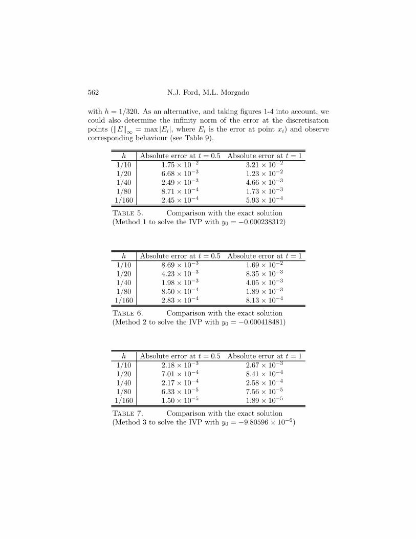
problem for the same value of y(0), then we expect to obtain small absoluteerrors as the step-size decreases. This, in fact, can be observed in Tables 5,6, 7 and 8, where for each value of the step-size h and for each initial valuesolver, the numerical solution is determined with y(0) obtained by shooting
562 N.J. Ford, M.L. Morgado
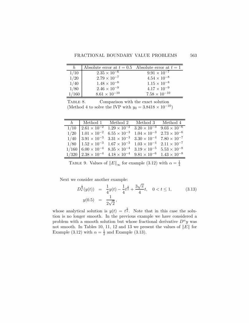
with h = 1/320. As an alternative, and taking figures 1-4 into account, wecould also determine the infinity norm of the error at the discretisationpoints (‖E‖∞ = max |Ei|, where Ei is the error at point xi) and observecorresponding behaviour (see Table 9).
h Absolute error at t = 0.5 Absolute error at t = 11/10 1.75 × 10⁻² 3.21 × 10⁻²
1/20 6.68 × 10⁻³ 1.23 × 10⁻²
1/40 2.49 × 10⁻³ 4.66 × 10⁻³
1/80 8.71 × 10⁻⁴ 1.73 × 10⁻³
1/160 2.45 × 10⁻⁴ 5.93 × 10⁻⁴
Table 5. Comparison with the exact solution(Method 1 to solve the IVP with y0 = −0.000238312)
h Absolute error at t = 0.5 Absolute error at t = 11/10 8.69 × 10⁻³ 1.69 × 10⁻²
1/20 4.23 × 10⁻³ 8.35 × 10⁻³
1/40 1.98 × 10⁻³ 4.05 × 10⁻³
1/80 8.50 × 10⁻⁴ 1.89 × 10⁻³
1/160 2.83 × 10⁻⁴ 8.13 × 10⁻⁴
Table 6. Comparison with the exact solution(Method 2 to solve the IVP with y0 = −0.000418481)
h Absolute error at t = 0.5 Absolute error at t = 11/10 2.18 × 10⁻³ 2.67 × 10⁻³
1/20 7.01 × 10⁻⁴ 8.41 × 10⁻⁴
1/40 2.17 × 10⁻⁴ 2.58 × 10⁻⁴
1/80 6.33 × 10⁻⁵ 7.56 × 10⁻⁵
1/160 1.50 × 10⁻⁵ 1.89 × 10⁻⁵
Table 7. Comparison with the exact solution(Method 3 to solve the IVP with y0 = −9.80596 × 10⁻⁶)
FRACTIONAL BOUNDARY VALUE PROBLEMS 563
h Absolute error at t = 0.5 Absolute error at t = 11/10 2.35 × 10⁻⁶ 9.91 × 10⁻⁷
1/20 2.79 × 10⁻⁷ 4.54 × 10⁻⁸
1/40 1.48 × 10⁻⁸ 1.15 × 10⁻⁸
1/80 2.46 × 10⁻⁹ 4.17 × 10⁻⁹
1/160 8.61 × 10⁻¹⁰ 7.58 × 10⁻¹⁰
Table 8. Comparison with the exact solution(Method 4 to solve the IVP with y0 = 3.8418 × 10⁻¹⁰)
h Method 1 Method 2 Method 3 Method 41/10 2.61 × 10⁻² 1.29 × 10⁻² 3.20 × 10⁻³ 9.03 × 10⁻⁶
1/20 1.01 × 10⁻² 6.55 × 10⁻³ 1.04 × 10⁻³ 2.73 × 10⁻⁶
1/40 3.91 × 10⁻³ 3.31 × 10⁻³ 3.30 × 10⁻⁴ 7.80 × 10⁻⁷
1/80 1.52 × 10⁻³ 1.67 × 10⁻³ 1.03 × 10⁻⁴ 2.11 × 10⁻⁷
1/160 6.00 × 10⁻⁴ 8.35 × 10⁻⁴ 3.19 × 10⁻⁵ 5.53 × 10⁻⁸
1/320 2.38 × 10⁻⁴ 4.18 × 10⁻⁴ 9.81 × 10⁻⁶ 1.43 × 10⁻⁸
Table 9. Values of ‖E‖∞ for example (3.12) with α = 14
Next we consider another example:
D12∗ (y(t)) =
14y(t) − 1
4t
32 +
3√
π
4t, 0 < t ≤ 1, (3.13)
y(0.5) =1
2√
2,
whose analytical solution is y(t) = t32 . Note that in this case the solu-
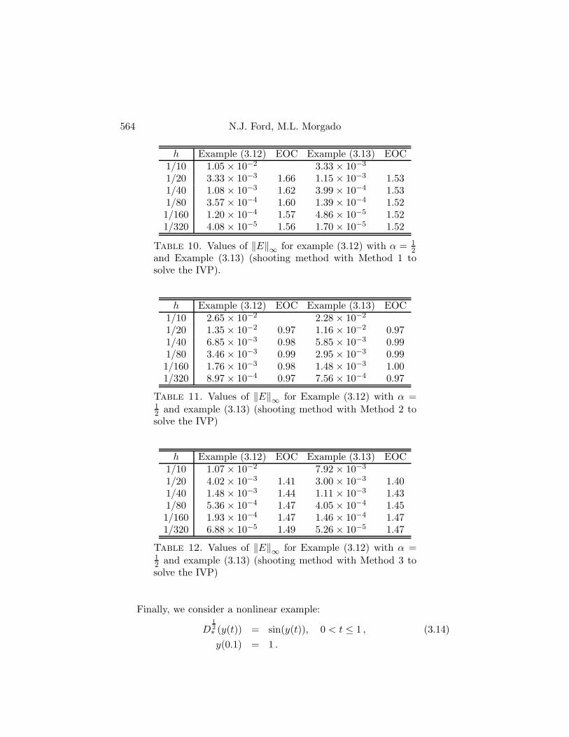
tion is no longer smooth. In the previous example we have considered aproblem with a smooth solution but whose fractional derivative Dαy wasnot smooth. In Tables 10, 11, 12 and 13 we present the values of ‖E‖ forExample (3.12) with α = 1
2 and Example (3.13).
564 N.J. Ford, M.L. Morgado
h Example (3.12) EOC Example (3.13) EOC1/10 1.05 × 10⁻² 3.33 × 10⁻³
1/20 3.33 × 10⁻³ 1.66 1.15 × 10⁻³ 1.531/40 1.08 × 10⁻³ 1.62 3.99 × 10⁻⁴ 1.531/80 3.57 × 10⁻⁴ 1.60 1.39 × 10⁻⁴ 1.521/160 1.20 × 10⁻⁴ 1.57 4.86 × 10⁻⁵ 1.521/320 4.08 × 10⁻⁵ 1.56 1.70 × 10⁻⁵ 1.52
Table 10. Values of ‖E‖∞ for example (3.12) with α = 12
and Example (3.13) (shooting method with Method 1 tosolve the IVP).
h Example (3.12) EOC Example (3.13) EOC1/10 2.65 × 10⁻² 2.28 × 10⁻²
1/20 1.35 × 10⁻² 0.97 1.16 × 10⁻² 0.971/40 6.85 × 10⁻³ 0.98 5.85 × 10⁻³ 0.991/80 3.46 × 10⁻³ 0.99 2.95 × 10⁻³ 0.991/160 1.76 × 10⁻³ 0.98 1.48 × 10⁻³ 1.001/320 8.97 × 10⁻⁴ 0.97 7.56 × 10⁻⁴ 0.97
Table 11. Values of ‖E‖∞ for Example (3.12) with α =12 and example (3.13) (shooting method with Method 2 tosolve the IVP)
h Example (3.12) EOC Example (3.13) EOC1/10 1.07 × 10⁻² 7.92 × 10⁻³
1/20 4.02 × 10⁻³ 1.41 3.00 × 10⁻³ 1.401/40 1.48 × 10⁻³ 1.44 1.11 × 10⁻³ 1.431/80 5.36 × 10⁻⁴ 1.47 4.05 × 10⁻⁴ 1.451/160 1.93 × 10⁻⁴ 1.47 1.46 × 10⁻⁴ 1.471/320 6.88 × 10⁻⁵ 1.49 5.26 × 10⁻⁵ 1.47
Table 12. Values of ‖E‖∞ for Example (3.12) with α =12 and example (3.13) (shooting method with Method 3 tosolve the IVP)
Finally, we consider a nonlinear example:
D12∗ (y(t)) = sin(y(t)), 0 < t ≤ 1 , (3.14)y(0.1) = 1 .
FRACTIONAL BOUNDARY VALUE PROBLEMS 565
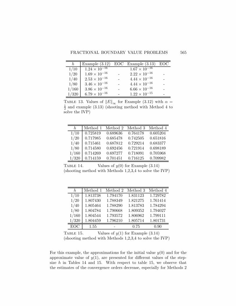
h Example (3.12) EOC Example (3.13) EOC1/10 1.24 × 10⁻¹⁶ 1.67 × 10⁻¹⁶
1/20 1.69 × 10⁻¹⁶ - 2.22 × 10⁻¹⁶ -1/40 2.53 × 10⁻¹⁶ - 4.44 × 10⁻¹⁶ -1/80 3.46 × 10⁻¹⁶ - 4.44 × 10⁻¹⁶ -1/160 3.86 × 10⁻¹⁶ - 6.66 × 10⁻¹⁶ -1/320 6.79 × 10⁻¹⁶ - 1.22 × 10⁻¹⁵ -
Table 13. Values of ‖E‖∞ for Example (3.12) with α =12 and example (3.13) (shooting method with Method 4 tosolve the IVP)
h Method 1 Method 2 Method 3 Method 41/10 0.725819 0.689636 0.764178 0.6052041/20 0.717985 0.685478 0.742505 0.6518161/40 0.715461 0.687812 0.729214 0.6833771/80 0.714580 0.692456 0.721914 0.6981891/160 0.714269 0.697277 0.718091 0.7059681/320 0.714159 0.701451 0.716125 0.709982
Table 14. Values of y(0) for Example (3.14)(shooting method with Methods 1,2,3,4 to solve the IVP)
h Method 1 Method 2 Method 3 Method 41/10 1.813738 1.794170 1.831123 1.7297821/20 1.807430 1.788349 1.821275 1.7614141/40 1.805464 1.788290 1.813783 1.7842941/80 1.804784 1.790668 1.809352 1.7940271/160 1.804544 1.793572 1.806962 1.7991111/320 1.804459 1.796210 1.805714 1.801731EOC 1.55 - 0.75 0.90
Table 15. Values of y(1) for Example (3.14)(shooting method with Methods 1,2,3,4 to solve the IVP)
For this example, the approximations for the initial value y(0) and for theapproximate value of y(1), are presented for different values of the step-size h in Tables 14 and 15. With respect to table 15, we observe thatthe estimates of the convergence orders decrease, especially for Methods 2
566 N.J. Ford, M.L. Morgado
and 3, in which it is necessary to use also a method for solving nonlinearequations. Here we have used the Newton’s method. Moreover, when usingMethod 2 we could not observe convergence for non small stepsizes.
4. Conclusions
For a class of boundary value problems for fractional differential equa-tions with order between 0 and 1, we have established sufficient conditionsfor the existence and uniqueness of the solution. As mentioned before,uniqueness results have already been obtained in [4], but in that paper theauthors did not consider the existence problem. Here we have shown thatboth existence and uniqueness results can be obtained.
With respect to the numerical methods, we have considered a proto-type method for solving the boundary value problems based on a shootingargument. We have considered four standard methods for solving the ini-tial value problems. Comparing the obtained numerical results, we see thatthe low order methods behave quite similarly for linear problems, in thesense that the expected estimated convergence orders (EOC) are observed.Concerning the higher order method used here (the Lubich method withconvergence order p = 3), we conclude by analyzing the obtained resultsthat although it is very accurate, it does not reveal the expected theoreticalconvergence order. We believe that these results have an easy explanation:it is known that these higher numerical methods should be used with someprudence, because instability may occur due to the cancelation of digitsin the linear system for the determination of the so-called starting weights([3]). Besides, as explained before, since, for each step size h we are shoot-ing on the initial value y(0) and the final approximate solution is obtainedby solving the initial value problem for that value of y(0), for different val-ues of h the computed solutions of the BVP are obtained with differentinitial values.
For all these reasons we believe that Method 1 ([6]) to solve the initialvalue problems when shooting on the unknown value of y(0) is the mostcompetitive method, since it is easy to implement, for linear and nonlinearproblems and the obtained numerical results illustrate that this methodperforms well when dealing with non-smooth solutions.
Acknowledgements
M. L. Morgado acknowledges financial support from FCT, Fundacaopara a Ciencia e Tecnologia, under grant SFRH/BPD/46530/2008.
FRACTIONAL BOUNDARY VALUE PROBLEMS 567
References
[1] M. Caputo, Elasticity e Dissipazione, Zanichelli, Bologna (1969).[2] K. Diethelm, An algorithm for the numerical solution of differential
equations of fractional order, Electr. Trans. Numer. Anal., 5 (1997),1–6.
[3] K. Diethelm, J.M. Ford, N.J. Ford and M. Weilbeer, Pitfalls in fastnumerical solvers for fractional differential equations, J. Comp. Appl.Mathem., 186, 2 (2006), 482–503.
[4] K. Diethelm, and N.J. Ford, Volterra integral equations and fractionalcalculus: Do neighbouring solutions intersect? Journal of IntegralEquations and Applications, to appear.
[5] K. Diethelm and N.J. Ford, Analysis of fractional differential equations.J. Math. Anal. Appl. 265 (2002), 229–248.
[6] K. Diethelm, N.J. Ford, and A.D. Freed, A.D., A predictor-correctorapproach for the numerical solution of fractional differential equations,Nonlinear Dynamics 29 (2002), 3–22.
[7] N.J. Ford and J.A. Connolly, Comparison of numerical methods forfractional differential equations, Commun. Pure Appl. Anal., 5, No 2(2006), 289–307.
[8] E. Hairer, Ch. Lubich and M. Schlichte, Fast numerical solution ofweakly singulat Volterra integral equations, J. Comp. Appl. Mathem.23 (1988), 87–98.
[9] S.G. Samko, A.A. Kilbas and O.I. Marichev, Fractional Integrals andDerivatives: Theory and Applications. Gordon and Breach, Yverdon(1993).
1 Department of MathematicsUniversity of ChesterParkgate Road, Chester, CH1 4BJ, UK
e-mail: [email protected] Received: May 30, 2011
2 CEMAT, IST, Lisbon andDepartment of MathematicsUniversity of Tras-os-Montes e Alto DouroQuinta de Prados 5001-801, Vila Real, PORTUGAL
e-mail: [email protected]
Please cite to this paper as published in:Fract. Calc. Appl. Anal., Vol. 14, No 4 (2011), pp. 554–567;DOI: 10.2478/s13540-011-0034-4


