
Internationale Mikroökonomik
Kurs, 3h, Do 14.00-17.00,
HS15.06
VO3: Faktorproportion und intersektoraler Handel: Heckscher-Ohlin
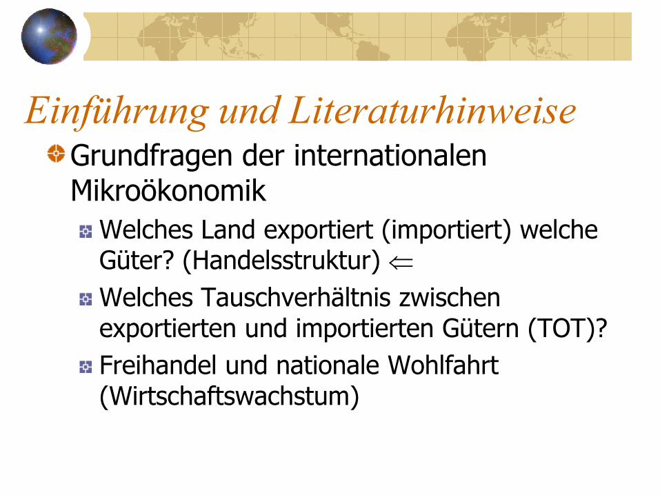
Einführung und Literaturhinweise Grundfragen der internationalen Mikroökonomik
Welches Land exportiert (importiert) welche Güter? (Handelsstruktur)
Welches Tauschverhältnis zwischen exportierten und importierten Gütern (TOT)?
Freihandel und nationale Wohlfahrt (Wirtschaftswachstum)

Einführung und Literaturhinweise
Bestimmungsfaktoren der Handelsstruktur: Faktorausstattung eines Landes
Libanius (314-393): Orationes
D. Hume (1752, Essay VI, Of the Jealousy of Trade)
E. Heckscher (1919)
B. Ohlin (1924)

Literaturhinweise
Farmer, K./Th. Vlk, Internationale Ökonomik. Eine Einführung in die Theorie und Empirie der Weltwirtschaft, 4. A., LIT-Verlag: Wien 2011, Kap. 9.
Feenstra, R., A.M. Taylor, International Economics, Worth Publishers, 3. Aufl., New York 2014, chap. 4.
Krugman, P./M. Obstfeld, Internationale Wirtschaft, 10. Aufl., 2014, Kap. 4.

Übersicht
Intertemporale Mikrofundierung
Internationale Kapitalmarkträumung
Heckscher-Ohlin-(Faktorproportionen-) Theorem
Analytisch
Grafisch

Intertemporale Mikrofundierung
Zwei Varianten intertemporaler Gleichgewichtsmodelle
Ramsey (1928)-Ansatz unendlich lang lebender Dynastien (ILA)Obstfeld und Rogoff (1996) Allais (1947)-Samuelson (1958)-Diamond (1965) Ansatz endlich lebender überlappender Generationen (Overlapping Generations = OLG) • De La Croix, Michel (2002), A Theory of Economic
Growth, Cambridge University Press • Farmer und Wendner (1997; 19992), Wachstum und
Außenhandel. Eine Einführung in die Gleichgewichtstheorie der Wachstums- und Außenhandelsdynamik, Physica: Heidelberg.
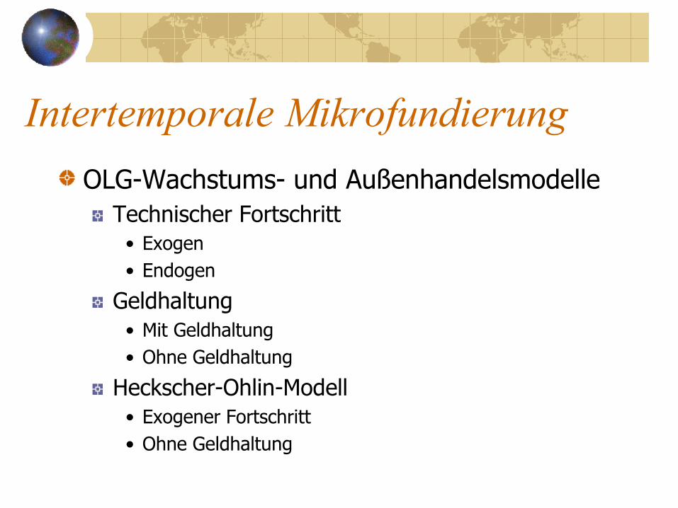
Intertemporale Mikrofundierung
OLG-Wachstums- und Außenhandelsmodelle
Technischer Fortschritt
• Exogen
• Endogen
Geldhaltung
• Mit Geldhaltung
• Ohne Geldhaltung
Heckscher-Ohlin-Modell
• Exogener Fortschritt
• Ohne Geldhaltung
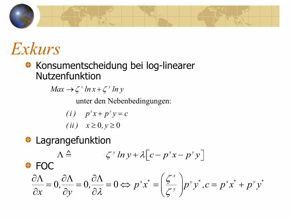
Exkurs Konsumentscheidung bei log-linearer Nutzenfunktion
Lagrangefunktion
FOC
unter den Nebenbedingungen:
0 0
x y
x y
Max ln x ln y
( i ) p x p y c
( ii ) x , y
x y x yln x ln y c p x p y
0 0 0x
x * y * x * y *
y, , p x p y ,c p x p y
x y
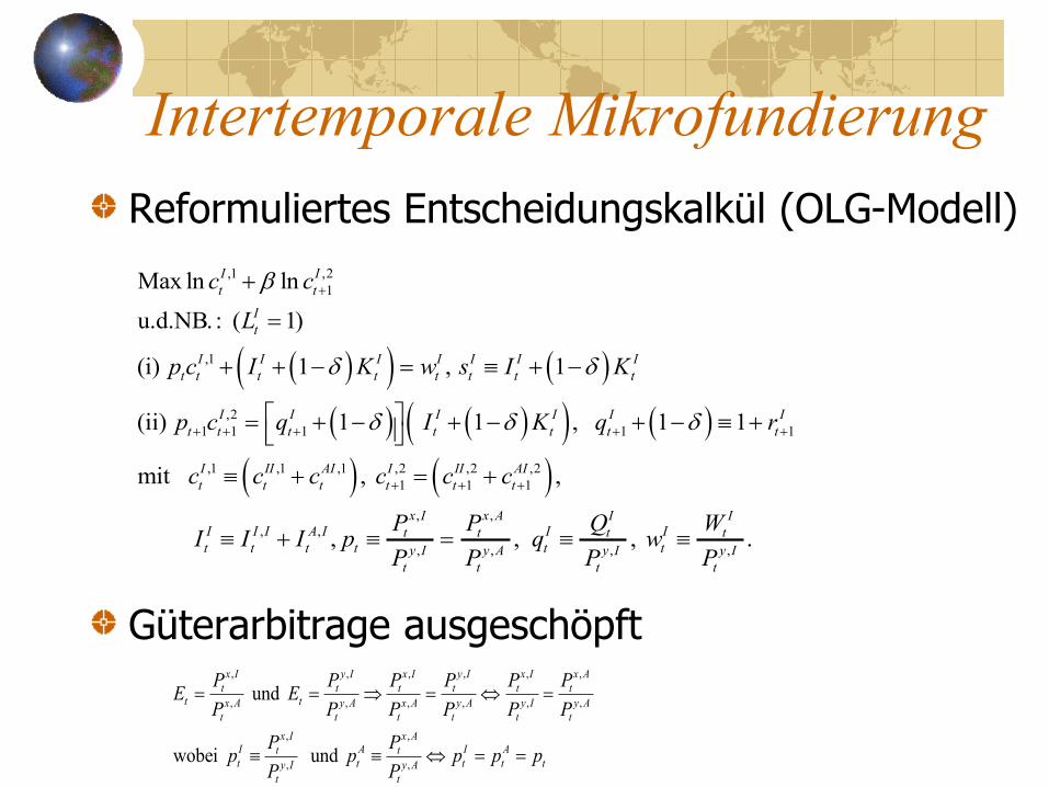
Intertemporale Mikrofundierung
Reformuliertes Entscheidungskalkül (OLG-Modell)
Güterarbitrage ausgeschöpft
, , , , , ,
, , , , , ,
, ,
, ,
und
wobei und
x I y I x I y I x I x A
t t t t t tt tx A y A x A y A y I y A
t t t t t t
x I x AI A I At tt t t t ty I y A
t t
P P P P P PE E
P P P P P P
P Pp p p p p
P P
,1 ,2
1
,1
,2
1 1 1 1 1
,1 ,1 ,1 ,2 ,2 ,2
1 1 1
,
Max ln ln
u.d.NB. : ( 1)
(i) 1 , 1
(ii) 1 1 , 1 1
mit , ,
I I
t t
I
t
I I I I I I I
t t t t t t t t
I I I I I I
t t t t t t t
I II AI I II AI
t t t t t t
I I I
t t
c c
L
p c I K w s I K
p c q I K q r
c c c c c c
I I
, ,
,
, , , ,, , , .
x I x A I I
A I I It t t t
t t t ty I y A y I y I
t t t t
P P Q WI p q w
P P P P

Intertemporale Mikrofundierung
Nutzenmaximierende Ersparnis
Intertemporale Budgetrestriktion
,1
,2
1 1 1 1 1
,1 ,2
1 1 1
,2,1 1 1
1
(i) 1 , 1
(ii) 1 1 , 1 1
(i)' , (ii)' 1
(iii)' .1
I I I I I I I
t t t t t t t t
I I I I I I
t t t t t t t
I I I I I I
t t t t t t t t
II It t
t t tI
t
p c I K w s I K
p c q I K q r
p c s w p c r s
p cp c w
r

Intertemporale Mikrofundierung
Nutzenmaximierende Ersparnis
Lagrangefunktion und FOC
,2
,1 ,2 ,1 1 1
1
1
,2
,11 1 1
,1 ,1 ,2 ,2
1 1 1 1
,2
1 1 1
,2 ,11 11
ln ln1
10, 0, 0
1 1
11
I
I I I I t t
t t t t t I
t
I
I It t t
t t t tI I I I I I
t t t t t t
I
t t t
I I It tt t t
p cL c c w p c
r
L L p L p cp w p c
c c c c r r
p p c
c rp c r
,2
,1 ,1 ,11 1
1
,1
1 1
,1 1 1
I I
I I I It t t
t t t t t t tI I
t
I
I I I I I It
t t t t t t t
p c wp c w p c p c
r
ws w p c w w w
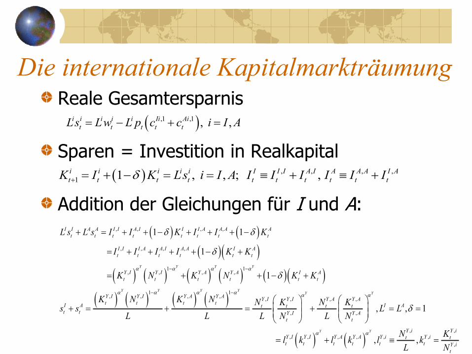
Die internationale Kapitalmarkträumung Reale Gesamtersparnis
Sparen = Investition in Realkapital
Addition der Gleichungen für I und A:
,1 ,1 , ,i i i i i Ii Ai
t t t t tLs Lw L p c c i I A
, , , ,
1 1 , , ; ,i i i i i I I I A I A A A I A
t t t t t t t t t tK I K Ls i I A I I I I I I
, , , ,
, , , ,
1 1, , , ,
1 1, , , ,
, ,
,
1 1
1
1Y Y Y Y
Y Y Y YY
I I A A I I A I I I A A A A
t t t t t t t t
I I I A A I A A I A
t t t t t t
Y I Y I Y A Y A I A
t t t t t t
Y I Y I Y A Y AY I Y I
t t t tI A t t
t t Y I
t
L s L s I I K I I K
I I I I K K
K N K N K K
K N K N N Ks s
L L L N
, ,
,
, ,
, , , , , ,
,
, , 1
, ,
Y
Y Y
Y A Y A
I At t
Y A
t
Y i Y i
Y I Y I Y A Y A Y i Y it t
t t t t t t Y i
t
N KL L
L N
N Kl k l k l k
L N
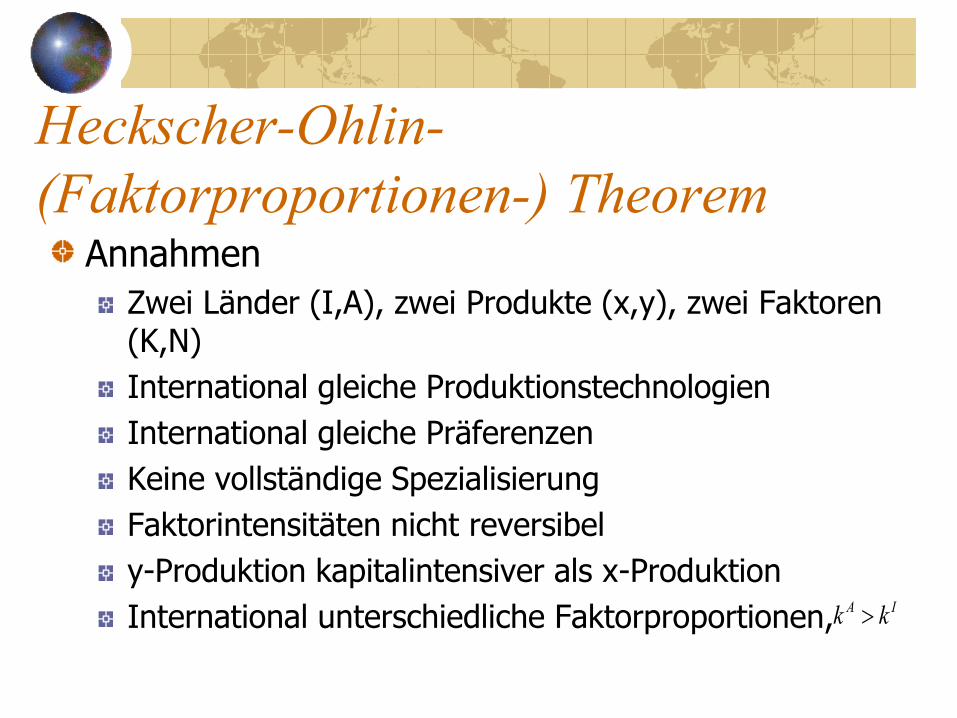
Heckscher-Ohlin-
(Faktorproportionen-) Theorem Annahmen
Zwei Länder (I,A), zwei Produkte (x,y), zwei Faktoren (K,N)
International gleiche Produktionstechnologien
International gleiche Präferenzen
Keine vollständige Spezialisierung
Faktorintensitäten nicht reversibel
y-Produktion kapitalintensiver als x-Produktion
International unterschiedliche Faktorproportionen, A Ik k

Heckscher-Ohlin-
(Faktorproportionen-) Theorem Aussage
Jedes Land exportiert (netto) jenes Produkt, das den in diesem Land reichlicher vorhandenen Faktor intensiv nutzt
Heckscher-Ohlin-
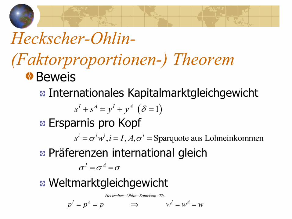
(Faktorproportionen-) Theorem Beweis
Internationales Kapitalmarktgleichgewicht
Ersparnis pro Kopf
Präferenzen international gleich
Weltmarktgleichgewicht
1I A I As s y y
, , , Sparquote aus Lohneinkommeni i i is w i I A
I A
.Heckscher Ohlin Samelson Th
I A I Ap p p w w w

Heckscher-Ohlin-
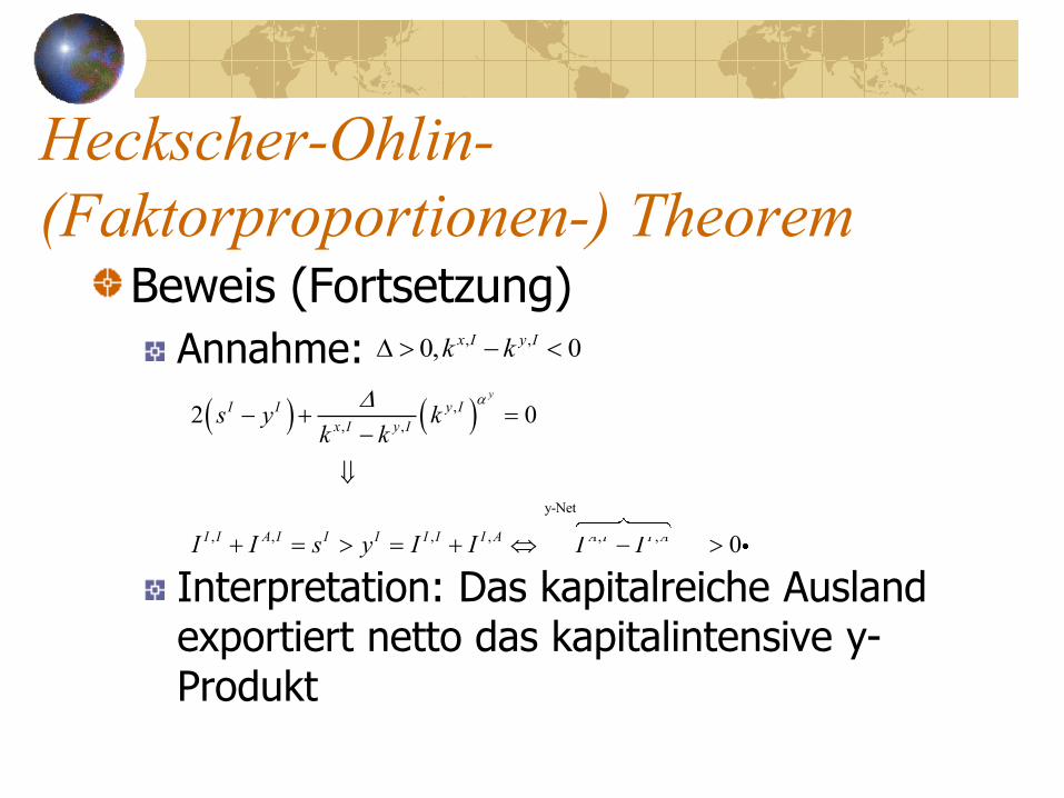
(Faktorproportionen-) Theorem Beweis (Fortsetzung)
Annahme:
2I A I I As s s y y
A Ik k
, 0A I A Ik k k k
, ,, , , , , ,
1 1, , , ,
,,
, , ,
1 1 1, , , , , ,
( )2 2 = , ,
2 =
+
y y
II
y y y
I x I I x II I A I y I y I x I x A y I y A
x I y I x I y I
yy
I x II x I
I y I y I y I
x I y I x I y I x I y I
I I
x
k k k ks y y s k k k k k k
k k k k
k kk ks k k k
k k k k k k
y yk
,
, ,
y
y I
I y Ik
k
Heckscher-Ohlin-
(Faktorproportionen-) Theorem Beweis (Fortsetzung)
Annahme:
Interpretation: Das kapitalreiche Ausland exportiert netto das kapitalintensive y-Produkt
, ,0, 0x I y Ik k
,
, ,
y-Nettoexport des Auslands
, , , , , ,
2 0
0
y
I I y I
x I y I
I I A I I I I I I A A I I A
s y kk k
I I s y I I I I

Heckscher-Ohlin-
(Faktorproportionen-) Theorem Grafische Darstellung I: Autarkie
Ip
Iy
Ix
Ix
MRSI
*
Ip
MRTI
*
Ix
*
Ix
I
tan I Ip
IP
Ay
MRSA
MRTA
Ax
AP
*
Ax
*
AxAx
Ausland
Inland
*
Ap
Abb 8.1
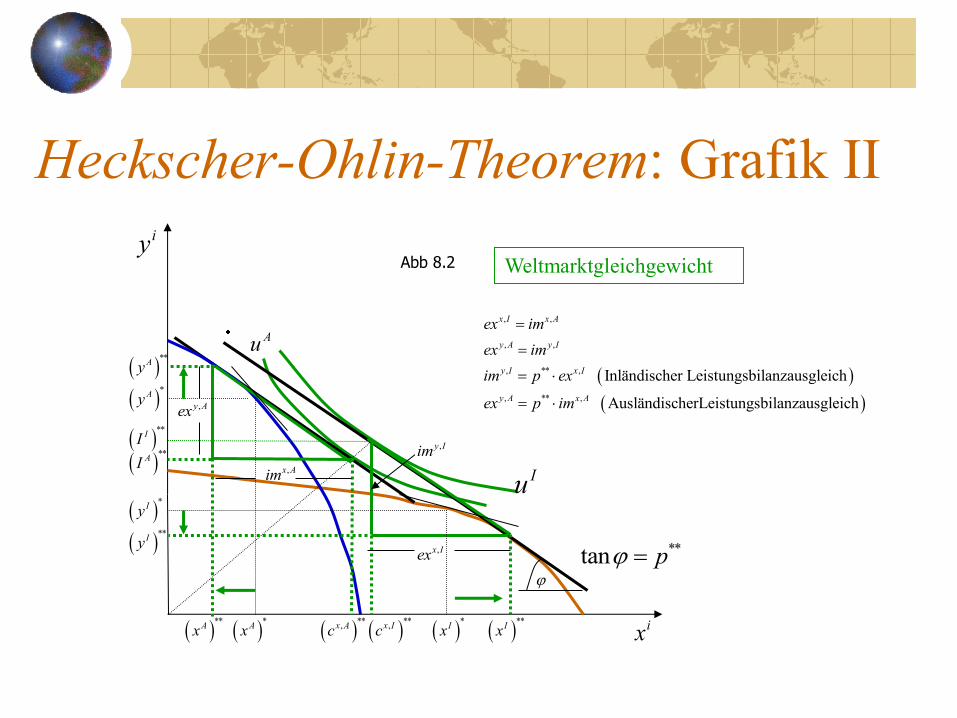
Heckscher-Ohlin-Theorem: Grafik II
ix
iy
Au
Iu
Weltmarktgleichgewicht
*
Ix **
Ix **
,x Ic
,x Iex
**
,x Ac *
Ax **
Ax
**
Iy
*
Iy
**
AI
**
II
*
Ay
**
Ay
**tan p
,y Aex
,x Aim
,y Iim
, ,
, ,
, ** ,
, ** ,
Inländischer Leistungsbilanzausgleich
AusländischerLeistungsbilanzausgleich
x I x A
y A y I
y I x I
y A x A
ex im
ex im
im p ex
ex p im
Abb 8.2

Heckscher-Ohlin-
(Faktorproportionen-) Theorem Weltmarktgleichgewicht alternativ betr.
,Ip p
**p
*
Ip
*
Ix **
,x Ic **
Ix Ix
Ap
p
Ax
*
Ap
**
,x Ac *
Ax **
Ax
,x Aim
,x Iex

Internationaler Markt
**p
,x Iex
p
,Ip p
**p
*
Ip
Ap
p
*
Ap
,x Aim
,x Iex
p
p
,x Aim
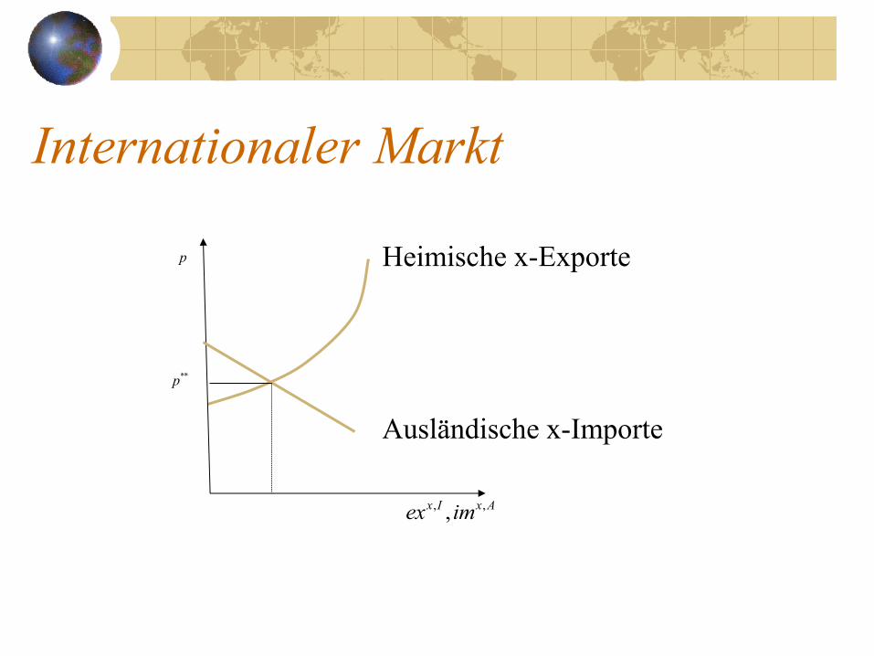
Internationaler Markt
p
**p
, ,,x I x Aex im
Heimische x-Exporte
Ausländische x-Importe

Heckscher-Ohlin-
(Faktorproportionen-) Theorem Tauschkurven OCi (Offer Curves)
,x Iex
,y Iim
tan ** Ip TOT
**
,x Iex
**
,y Iim
,x Iex
,y Iim
0
0
IOC
AOC
,
,
y I
y A
im
e
, ,,x I x Aex im ** **
, ,x I x Aex im
** **
, ,y I y Aim ex


