
Interpreting Coefficients in Marginal vs. Mixed ModelsZACHARY BINNEY
EPI 750, SPRING 2019

Interpreting βs in Correlated Data Models
Model Type Outcome is… Interpret βs as…
Marginal Continuous (MLM) Population-average change
Marginal Categorical/Count (GEE) Population-average change
Mixed Continuous (LMM) Population-average change OR subject-specific change (identical)
Mixed Categorical/Count(GLMM)
Subject-specific change

Population-Average vs. Subject-Specific Interpretations• In marginal (any outcome) or linear mixed models (continuous outcomes),
these are the same thing
• In GLMMs for categorical or count outcomes, they are not
• Why?
• Let’s consider a simple example

Population-Average vs. Subject-Specific Interpretations• A study of 3 people (A, B, and C) that we treat with, say, aspirin to prevent, say, heart attacks
• Have different baseline risks that we account for with a random intercept
Individual Baseline
Risk
Post-
Treatment Risk
RD (Linear
Model)
A 0.80 0.67 -0.13
B 0.50 0.33 -0.17
C 0.20 0.11 -0.09
Population
Average
0.50 0.37 -0.13
Unknown in reality, assuming we know
for our example
Source: Adapted from Fitzmaurice, Laird, and Ware. Applied Longitudinal Data Analysis..

Population-Average vs. Subject-Specific Interpretations
• Say we model risk using a linear mixed model (questionable, but bear with me):
• 𝑅𝑖𝑠𝑘𝑖𝑗 = 𝛽0 + 𝑏0𝑖 + 𝛽1 𝑃𝑜𝑠𝑡𝑖𝑗 where Post = 1 if post-treatment, 0 if baseline
• Average of individual risk differences: −0.13+ −0.17 +(−0.09)
3= −𝟎. 𝟏𝟑
• Difference in population-average risks: 0.37 − 0.50 = −𝟎. 𝟏𝟑
• 𝛽1 = 0.13 and can be interpreted in two ways:
• After treating everyone with aspirin, the average risk of a heart attack in the population dropped by 0.13.
• After treatment with aspirin, the typical subject exhibited a drop in the risk of heart attack of 0.13.
Individual Baseline Risk
of D
Post-Treatment
Risk of D
RD (Linear
Model)
A 0.80 0.67 -0.13
B 0.50 0.33 -0.17
C 0.20 0.11 -0.09
Population
Average
0.50 0.37 -0.13
Source: Adapted from Fitzmaurice, Laird, and Ware. Applied Longitudinal Data Analysis..
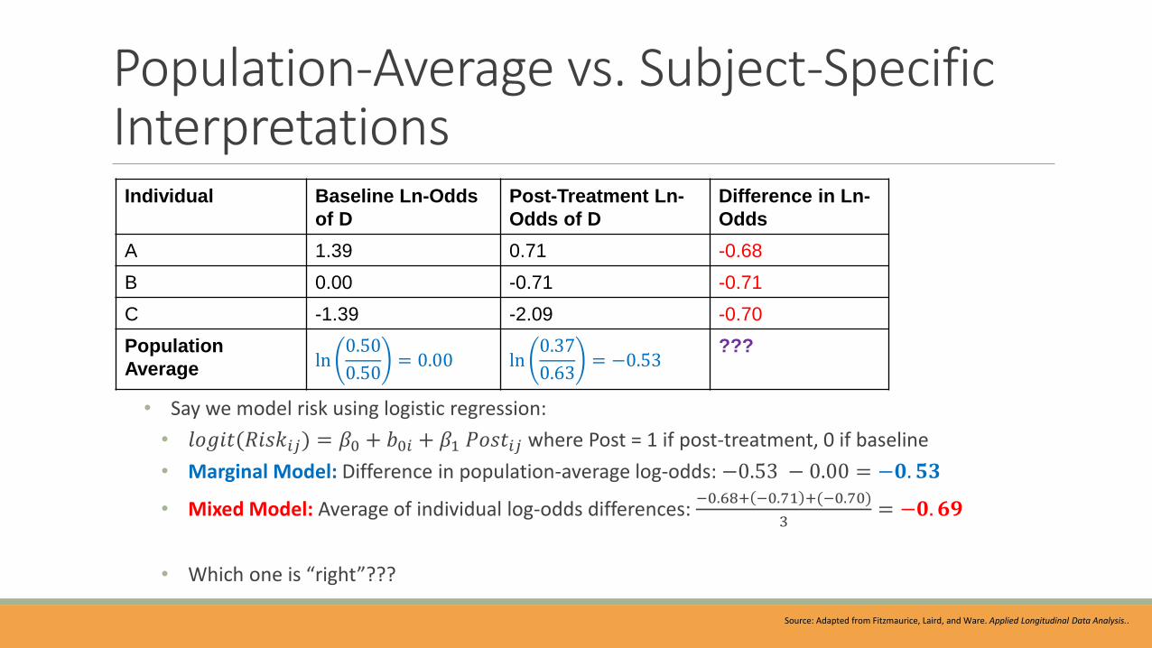
Population-Average vs. Subject-Specific Interpretations
• Say we model risk using logistic regression:
• 𝑙𝑜𝑔𝑖𝑡(𝑅𝑖𝑠𝑘𝑖𝑗) = 𝛽0 + 𝑏0𝑖 + 𝛽1 𝑃𝑜𝑠𝑡𝑖𝑗 where Post = 1 if post-treatment, 0 if baseline
• Marginal Model: Difference in population-average log-odds: −0.53 − 0.00 = −𝟎. 𝟓𝟑
• Mixed Model: Average of individual log-odds differences: −0.68+ −0.71 +(−0.70)
3= −𝟎. 𝟔𝟗
• Which one is “right”???
Individual Baseline Ln-Odds
of D
Post-Treatment Ln-
Odds of D
Difference in Ln-
Odds
A 1.39 0.71 -0.68
B 0.00 -0.71 -0.71
C -1.39 -2.09 -0.70
Population
Average ln0.50
0.50= 0.00 ln
0.37
0.63= −0.53
???
Source: Adapted from Fitzmaurice, Laird, and Ware. Applied Longitudinal Data Analysis..

Population-Average vs. Subject-Specific Interpretations
• Which one is “right?”
• Would you believe…both? It depends on your question!
• Marginal model →𝛽1 = −0.53→ OR = 0.59
• Interpretation: After treating everyone with aspirin, the odds of a heart attack were 41% lower, on average, across our study population.
• Mixed model →𝛽1 = −0.69→ OR = 0.50
• Interpretation: After treatment with aspirin, the typical subject exhibited a 50% reduction in their odds of a heart attack.
Individual Baseline Ln-Odds
of D
Post-Baseline Ln-
Odds of D
Difference in Ln-
Odds
A 1.39 0.71 -0.68
B 0.00 -0.71 -0.71
C -1.39 -2.09 -0.70
Population
Average ln0.50
0.50= 0.00 ln
0.37
0.63= −0.53
−𝟎. 𝟓𝟑 or −𝟎. 𝟔𝟗
Source: Adapted from Fitzmaurice, Laird, and Ware. Applied Longitudinal Data Analysis..
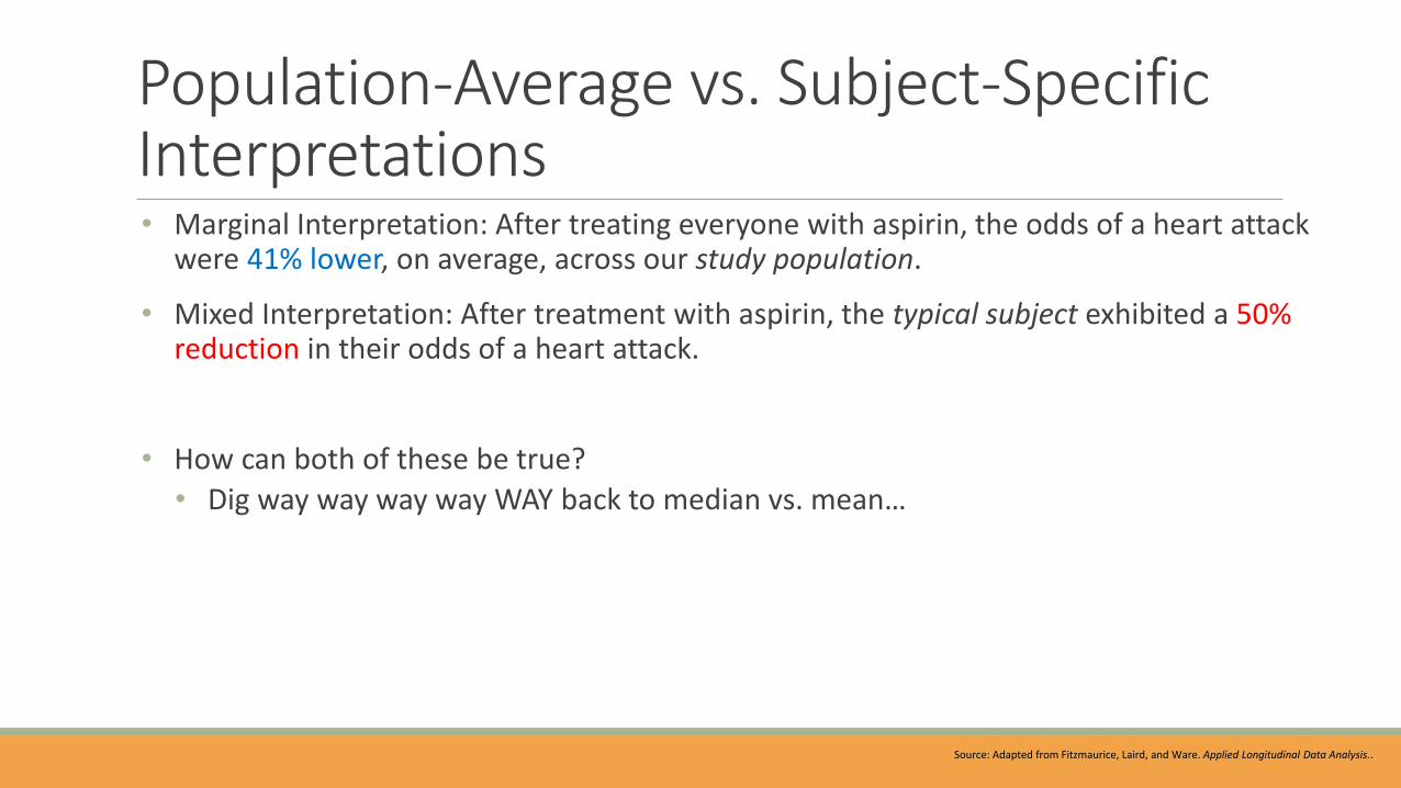
Population-Average vs. Subject-Specific Interpretations• Marginal Interpretation: After treating everyone with aspirin, the odds of a heart attack
were 41% lower, on average, across our study population.
• Mixed Interpretation: After treatment with aspirin, the typical subject exhibited a 50% reduction in their odds of a heart attack.
• How can both of these be true?
• Dig way way way way WAY back to median vs. mean…
Source: Adapted from Fitzmaurice, Laird, and Ware. Applied Longitudinal Data Analysis..

Population-Average vs. Subject-Specific Interpretations
Source: Adapted from Fitzmaurice, Laird, and Ware. Applied Longitudinal Data Analysis..
“Median” = log-odds of D (at baseline) for a “typical” individual
“Mean” = average log-odds of D (at baseline) in the population
Median = Mean
“Median” = probability of D (at baseline) for a “typical” individual
“Mean” = prevalence of disease (at baseline) in the population
“Median”≠ “Mean”
Marginal Model contrasts population means.
Mixed model contrasts population medians (i.e. “typical” subject at baseline
vs. post-baseline)

Population-Average vs. Subject-Specific Interpretations
Source: Adapted from Fitzmaurice, Laird, and Ware. Applied Longitudinal Data Analysis..
A linear model assumes these distributions are normal
(conditional on all predictors) – not skewed as shown here. So linear model assumes mean = median!
...but after treatment, we’re left with a bunch of low-risk people, with a few remaining high-risk
After treatment, the log-odds of disease for everyone shift
uniformly lower...
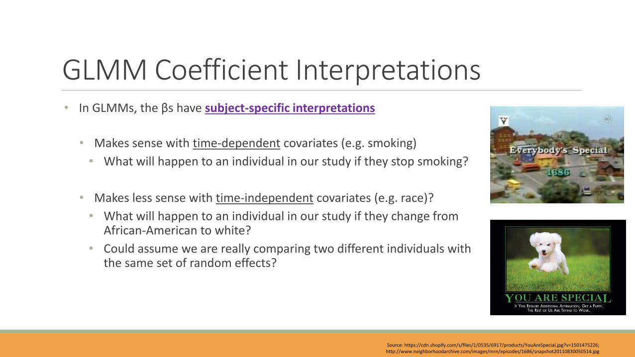
GLMM Coefficient Interpretations• In GLMMs, the βs have subject-specific interpretations
• Makes sense with time-dependent covariates (e.g. smoking)
• What will happen to an individual in our study if they stop smoking?
• Makes less sense with time-independent covariates (e.g. race)?
• What will happen to an individual in our study if they change from African-American to white?
• Could assume we are really comparing two different individuals with the same set of random effects?
Source: https://cdn.shopify.com/s/files/1/0535/6917/products/YouAreSpecial.jpg?v=1501475226; http://www.neighborhoodarchive.com/images/mrn/episodes/1686/snapshot20110830050514.jpg

Example: Onychomycosis Study

Onychomycosis Trial Example• Randomized trial of two oral antifungal treatments K = 294 subjects
• N = 1,908 measures of onycholysis (separation of nail from nail bed)
• ni = 1 to 7, unbalanced
• Outcome: Y = none/mild or moderate/severe onycholysis (0/1), measured at time = 0 (baseline) and approximately 4, 8, 12, 24, 36, and 48 weeks
• For this example, we are limiting to just the first 24 weeks
• Exposure: oral antifungal treatment (Itraconazole = 0, Terbinafine = 1)
• No controls
• Covariates: None
• Research Question: How does terbinafine impact the risk of moderate/severe onycholysis over time?
Source: Fitzmaurice, Laird, and Ware. Applied Longitudinal Data Analysis. https://content.sph.harvard.edu/fitzmaur/ala2e/. De Backer, M., et al (1998). Journal of the American Academy of Dermatology, 38, 57-63.

Marginal Model for Onychomycosis DataGEE Model, CS working correlation structure:
𝑙𝑜𝑔𝑖𝑡(𝐸(𝑌𝑖𝑗)) = 𝛽0 + 𝛽1𝑇𝑖𝑚𝑒𝑖𝑗
Just looking at terbafine to simplify example

Random Intercept Model for Onychomycosis Data
Model with Random Intercept for Subject:
𝑙𝑜𝑔𝑖𝑡(𝐸(𝑌𝑖𝑗|𝑏𝑖)) = 𝛽0 + 𝑏0𝑖 + 𝛽1𝑇𝑖𝑚𝑒𝑖𝑗 where 𝑏0𝑖 ~ 𝑁 0, 𝜎02 𝑖𝑖𝑑
Just looking at terbafine to simplify example
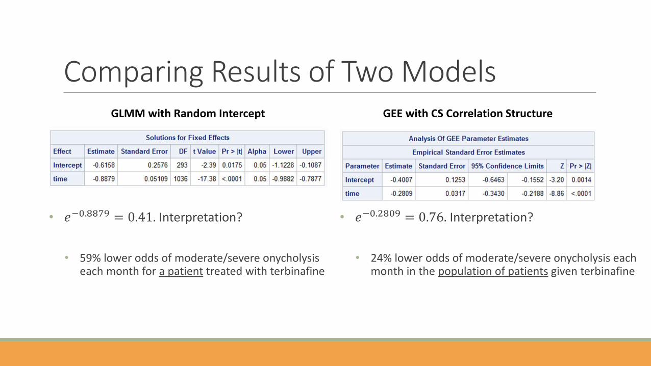
Comparing Results of Two ModelsGLMM with Random Intercept GEE with CS Correlation Structure
• 𝑒−0.8879 = 0.41. Interpretation?
• 59% lower odds of moderate/severe onycholysis each month for a patient treated with terbinafine
• 𝑒−0.2809 = 0.76. Interpretation?
• 24% lower odds of moderate/severe onycholysis each month in the population of patients given terbinafine

Comparing Results of Two ModelsGLMM with Random Intercept GEE with CS Correlation Structure
• 59% lower odds of moderate/severe onycholysis each month for a patient treated with terbinafine
• 24% lower odds of moderate/severe onycholysis each month in the population of patients given terbinafine
• Which of these is right?
• Both!
• …Zach, that’s not helpful. I have a study to do, which model should I use?
• It depends! On your research question!
• Do you want to know what happens to your study population, or to a typical individual in it?
• Research Question: How does terbafine impact the risk of moderate/severe onycholysis over time? Could ask it either way; it’s up to you

Summary

Key Points• βs in marginal models have a population-average interpretation
• e.g. 24% lower odds of moderate/severe onycholysis each month in the population of patientstreated with terbafine
• βs in mixed models have a subject-specific interpretation
• e.g. 59% lower odds of moderate/severe onycholysis each month for a patient treated with terbafine


