
Magnetism to Spintronics
Introduction to Solid State Physics Kittel 8th ed Chap. 11-13,
Condensed Matter Physics
Marder 2nd ed Chap. 24-26,
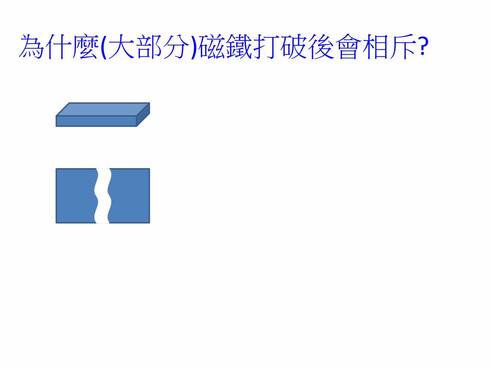
為什麼(大部分)磁鐵打破後會相斥?

Cooperative phenomena
• Elementary excitations in solids describe the response of a solid to a perturbation
– Quasiparticles
usually fermions, resemble the particles that make the system, e.g. quasi-electrons
– Collective excitations
usually bosons, describe collective motions
use second quantization with Fermi-Dirac or Bose- Einstein statistics

Magnetism
• the Bohr–van Leeuwen theorem
when statistical mechanics and classical mechanics are applied consistently, the thermal average of the magnetization is always zero.
• Magnetism in solids is solely a quantum mechanical effect
• Origin of the magnetic moment:
– Electron spin 𝑆
– Electron orbital momentum 𝐿
• From (macroscopic) response to external magnetic field 𝐻
– Diamagnetism < 0, χ~1 × 10⁻⁶, insensitive to temperature
– Paramagnetism > 0, χ =𝐶
𝑇 Curie law
χ =𝐶
𝑇+Δ Curie-Weiss law
– Ferromagnetism exchange interaction (quantum)

物質的磁性分類
巨觀: 順磁性 逆磁性 Paramagnetism diamagnetism
微觀: 鐵磁性 反鐵磁性 亞鐵磁性 Ferromagnetism Antiferromagnetism Ferrimagnetism


為什麼(大部分)磁鐵打破後會相斥?
N
N
N N
S
S
S S
?

• Classical and quantum theory for diamagnetism – Calculate 𝑟2
• Classical and quantum theory for paramagnetism – Superparamagnetism, Langevin function
– Hund’s rules
– Magnetic state 𝐿𝐽2𝑆+1
– Crystal field
– Quenching of orbital angular momentum Lz
• Angular momentum operator
• Spherical harmonics
– Jahn-Teller effect
– Paramagnetic susceptibility of conduction electrons

• Ferromagnetism
– Microscopic – ferro, antiferro, ferri magnetism
– Exchange interaction
– Exchange splitting – source of magnetization
two-electron system spin-independent Schrodinger equation
– Type of exchange: direct exchange, super exchange, indirect exchange, itinerant exchange
– Spin Hamiltonian and Heisenberg model
– Molecular-field (mean-field) approximation

Critical phenomena Universality. Divergences near the critical point are identical in a variety of apparently different physical systems and also in a collection of simple models. Scaling. The key to understanding the critical point lies in understanding the relationship between systems of different sizes. Formal development of this idea led to the renormalization group of Wilson (1975).
Landau Free Energy
F(M, T) =A0(T)+A2(T)M 2 +A4(T)M 4 +HM.
F
M
𝑡 ≡𝑇 − 𝑇𝐶
𝑇𝐶
F = a2tM 2 + a4M 4 + HM.
Molar heat capacities of four ferromagnetic copper salts versus scaled temperature T/Tc. [Source Jongh and Miedema (1974).]

Correspondence between Liquids and Magnets
• Specific Heat— • Magnetization and Density— • Compressibility and Susceptibility— • Critical Isotherm— • Correlation Length — • Power-Law Decay at Critical Point—
Summary of critical exponents, showing correspondence between fluid-gas systems, magnetic systems, and the three-dimensional Ising model.
Relations Among Exponents
𝛼 + 2𝛽 + 𝛾 = 2
𝛿 = 1 + 𝛾𝛽
2 − 𝜂 𝜈 = 𝛾
2 − 𝛼 = 3𝜈

• Stoner band ferromagnetism Teodorescu, C. M.; Lungu, G. A. (November 2008). "Band ferromagnetism in systems of variable dimensionality". Journal of Optoelectronics and Advanced Materials 10 (11): 3058–3068.

鐵磁性元素 : 鐵 Fe, 鈷 Co, 鎳 Ni, 釓 Gd, 鏑 Dy, 錳 Mn, 鈀 Pd ??
Elements with ferromagnetic properties 合金, alloys
錳氧化物 MnOx
13

Tetrahedron Cube hexahedron Octahedron Dodecahedron Icosahedron
Platonic solid From Wikipedia
In geometry, a Platonic solid is a convex polyhedron that is regular, in the
sense of a regular polygon. Specifically, the faces of a Platonic solid are
congruent regular polygons, with the same number of faces meeting at each
vertex; thus, all its edges are congruent, as are its vertices and angles.
There are precisely five Platonic solids (shown below):
The name of each figure is derived from its number of faces: respectively 4,
6, 8, 12, and 20.
The aesthetic beauty and symmetry of the Platonic solids have made them a
favorite subject of geometers for thousands of years. They are named for the
ancient Greek philosopher Plato who theorized that the classical elements were
constructed from the regular solids.

Solar system
s, p electron orbits
Orbital viewer 15
Electronic orbit

Resonance
One-dimensional
Two-dimensional
Hydrogen atom Three-dimensional

s, p electron orbital
Orbital viewer 17
3d transition metals: Mn atom has 5 d electrons Bulk Mn is NOT magnetic
Co atom has 5 d electrons and 2 d electrons
Bulk Co is magnetic.
3d electron distribution in real space

d orbitals
Crystal-field splitting

Stern-Gerlach Experiment
There are two kinds of electrons: spin-up and spin-down.

Stoner criterion for ferromagnetism:
For the non-magnetic state there are identical density of states
for the two spins.
For a ferromagnetic state, N↑ > N↓. The polarization is
indicated by the thick blue arrow.
I N(EF) > 1, I is the Stoner exchange parameter and
N(EF) is the density of states at the Fermi energy.
Schematic plot for the energy band structure of 3d transition metals.
20 Teodorescu and Lungu, "Band ferromagnetism in systems of variable dimensionality". J Optoelectronics and Adv. Mat. 10, 3058–3068 (2008).


Stoner–Wohlfarth model
The Stoner–Wohlfarth model is a widely used model for the magnetization of single-domain ferromagnets.[1] It is a simple example of magnetic hysteresis and is useful for modeling small magnetic particles in magnetic storage, biomagnetism, rock magnetism and paleomagnetism.
Ku is the anisotropy parameter V is the volume of the magnet, Ms is the saturation magnetization, and μ0 is the vacuum permeability

Berry Phase Aharonov-Bohm Effect
Electrons traveling around a flux tube suffer a phase
change and can interfere with themselves even if
they only travel through regions where B = 0.
(B) An open flux tube is not experimentally
realizable, but a small toroidal magnet with no flux
leakage can be constructed instead.
Electron hologram showing interference
fringes of electrons passing through small
toroidal magnet. The magnetic flux passing
through the torus is quantized so as to produce
an integer multiple of phase change in the
electron wave functions. The electron is
completely screened from the magnetic
induction in the magnet. In (A) the phase
change is 0, while in (B) the phase change is .
[Source: Tonomura (1993), p. 67.]
Φ = 𝑑2𝑟 𝐵𝑧 = 𝑑𝑟 ∙ 𝐴
𝐴𝜙 =Φ
2𝜋𝑟

Parallel transport of a vector along a closed path on the sphere S2 leads to a geometric phase between initial and final state.
Real-space Berry phases: Skyrmion soccer (invited)
Karin Everschor-Sitte and Matthias Sitte
Journal of Applied Physics 115, 172602 (2014); doi: 10.1063/1.4870695

25
Parameter dependent system:
Berry phase formalism for intrinsic Hall effects
Berry phase [Berry, Proc. Roy. Soc. London A 392, 451 (1984)]
Adiabatic theorem:
Geometric phase:
From Prof. Guo Guang-Yu

26
From Prof. Guo Guang-Yu Well defined for a closed path
Stokes theorem
Berry Curvature

27
From Prof. Guo Guang-Yu
Vector potential
Analogies
Berry curvature
Geometric phase
Berry connection
Chern number Dirac monopole
Aharonov-Bohm phase
Magnetic field

28
From Prof. Guo Guang-Yu
Semiclassical dynamics of Bloch electrons Old version [e.g., Aschroft, Mermin, 1976]
New version [Marder, 2000]
Berry phase correction [Chang & Niu, PRL (1995), PRB (1996)]
(Berry curvature)

Demagnetization factor D can be solved analytically in some cases, numerically in others
For an ellipsoid Dx + Dy + Dz = 1 (SI units) Dx + Dy + Dz = 4 (cgs units)
Solution for Spheroid a = b c
1. Prolate spheroid (football shape) c/a = r > 1 ; a = b , In cgs units
Limiting case r >> 1 ( long rod )
2. Oblate Spheroid (pancake shape) c/a = r < 1 ; a = b
Limiting case r >> 1 ( flat disk)
𝐷𝑎 = 𝐷𝑏 =4𝜋 − 𝐷𝑐
2
c a
a
Note: you measure 2M without knowing the sample
𝐷𝑐 = 4𝜋𝑟2 ln 2𝑟 − 1 ≪ 1
𝐷𝑎 = 𝐷𝑏 = 2𝜋
𝐷𝑐 = 4𝜋𝑟2−1
𝑟
𝑟2−1ln 𝑟 + 𝑟2 − 1 − 1
𝐷𝑎 = 𝐷𝑏 =4𝜋 − 𝐷𝑐
2 𝐷𝑐 = 4𝜋
1−𝑟2 1 − 𝑟
1−𝑟2cos−1 𝑟
𝐷𝑐 = 4𝜋
𝐷𝑎 = 𝐷𝑏 = 𝜋 2𝑟 ≪ 1 Note: you measure 4M without knowing the sample

Surface anisotropy
• 𝐸𝑒𝑥 : 2𝐽𝑆𝑖 ∙ 𝑆𝑗
• 𝐸𝑍𝑒𝑒𝑚𝑎𝑛 : 𝑀 ∙ 𝐻
• 𝐸𝑚𝑎𝑔 : 1
8𝜋 𝐵2𝑑𝑉
• 𝐸𝑎𝑛𝑖𝑠𝑜𝑡𝑟𝑜𝑝𝑦
For hcp Co= 𝐾1′ sin2 𝜃 + 𝐾2′ sin
4 𝜃 For bcc Fe = 𝐾1 𝛼1
2𝛼22 + 𝛼2
2𝛼32 + 𝛼3
2𝛼12 + 𝐾2 𝛼1
2𝛼22𝛼3
2 𝛼𝑖 : directional cosines
Surface anisotropy 𝐾eff =2𝐾𝑆
𝑡+ 𝐾𝑉 𝐾eff ∙ 𝑡 = 2𝐾𝑆 + 𝐾𝑉 ∙ 𝑡
𝐸 = 𝐸𝑒𝑥𝑐ℎ𝑎𝑛𝑔𝑒 + 𝐸𝑍𝑒𝑒𝑚𝑎𝑛 + 𝐸𝑚𝑎𝑔 + 𝐸𝑎𝑛𝑖𝑠𝑜𝑡𝑟𝑜𝑝𝑦 + ⋯

Ferromagnetic domains
For a 180 Bloch wall rotated in N+1 atomic planes 𝑁∆𝐸𝑒𝑥= 𝑁(𝐽𝑆2𝜋
𝑁
2
)
Wall energy density 𝜎𝑤 = 𝜎𝑒𝑥 + 𝜎𝑎𝑛𝑖𝑠 ≈ 𝐽𝑆2𝜋2/(𝑁𝑎2) + 𝐾𝑁𝑎 𝑎 : lattice constant
𝜕𝜎𝑤/𝜕𝑁 ≡ 0, 𝑁 = [𝐽𝑆2𝜋2/(𝐾𝑎3)] ≈ 300 in Fe
𝜎𝑤 = 2𝜋 𝐾𝐽𝑆2/𝑎 ≈ 1 erg/cm2 in Fe
Wall width 𝑁𝑎 = 𝜋 𝐽𝑆2/𝐾𝑎 ≡ 𝜋𝐴
𝐾 𝐴 = 𝐽𝑆2/𝑎 Exchange stiffness constant ,
– competition between exchange, anisotropy, and magnetic energies.
– Bloch wall: rotation out of the plane of the two spins
– Neel wall: rotation within the plane of the two spins

32
Domain wall energy versus thickness D of Ni80Fe20 thin films
N < B ~ 50nm
Thick films have Bloch walls
Thin films have Neel walls
Cross-tie walls show up in
between.
A=10-6 erg/cm
K=1500 erg/cm3
D
D 50nm
Cross-tie zone
N
B
N < B

Magnetic Resonance • Nuclear Magnetic Resonance (NMR)
– Line width
– Hyperfine Splitting, Knight Shift
– Nuclear Quadrupole Resonance (NQR)
• Ferromagnetic Resonance (FMR) – Shape Effect
– Spin Wave resonance (SWR)
• Antiferromagnetic Resonance (AFMR)
• Electron Paramagnetic Resonance (EPR or ESR) – Exchange narrowing
– Zero-field Splitting
• Maser
What we can learn:
• From absorption fine structure electronic structure of single defects
• From changes in linewidth relative motion of the spin to the surroundings
• From resonance frequency internal magnetic field
• Collective spin excitations

FMR
Shape effect:
internal magnetic field
ℏ𝑑𝑰
𝑑𝑡= 𝝁 × 𝑩
𝑑𝝁
𝑑𝑡= 𝛾𝝁 × 𝑩
𝑑𝑴
𝑑𝑡= 𝛾𝑴 × 𝑩 𝝁 = 𝛾ℏ𝑰
𝐵𝑥𝑖 = 𝐵𝑥
0 − 𝑁𝑥𝑀𝑥 𝐵𝑦𝑖 = 𝐵𝑦
0 − 𝑁𝑦𝑀𝑦 𝐵𝑧𝑖 = 𝐵𝑧
0 − 𝑁𝑧𝑀𝑧
𝑑𝑀𝑥
𝑑𝑡= 𝛾 𝑀𝑦𝐵𝑧
𝑖 − 𝑀𝑧𝐵𝑦𝑖 = 𝛾[𝐵0 + 𝑁𝑦 − 𝑁𝑧 𝑀]𝑀𝑦
𝑑𝑀𝑦
𝑑𝑡= 𝛾 𝑀 −𝑁𝑥𝑀𝑥 − 𝑀𝑥 𝐵0 − 𝑁𝑧𝑀 = −𝛾[𝐵0 + 𝑁𝑥 − 𝑁𝑧 𝑀]𝑀𝑥
𝑑𝑀𝑧
𝑑𝑡= 0 𝑀𝑧= 𝑀
𝑖𝜔 𝛾[𝐵0 + 𝑁𝑦 − 𝑁𝑧 𝑀]
−𝛾[𝐵0 + 𝑁𝑥 − 𝑁𝑧 𝑀] 𝑖𝜔= 0
𝜔02 = 𝛾2[𝐵0 + 𝑁𝑦 − 𝑁𝑧 𝑀][𝐵0 + 𝑁𝑥 − 𝑁𝑧 𝑀]
Equation of motion of a magnetic moment 𝝁 in an external field 𝐵0
To first order
Uniform mode
Landau-Lifshitz-Gilbert (LLG) equation
𝑑𝑴
𝑑𝑡= −𝛾𝑴 × 𝑯eff + 𝛼𝑴 ×
𝑑𝑴
𝑑𝑡

Sphere flat plate with perpendicular field flat plate with in-plane field
B0 B0
𝑁𝑥 = 𝑁𝑦 = 𝑁𝑧
𝜔0 = 𝛾 𝐵0
𝑁𝑥 = 𝑁𝑦 = 0 𝑁𝑧 = 4𝜋
𝜔0 = 𝛾 (𝐵0−4𝜋𝑀)
𝑁𝑥 = 𝑁𝑧 = 0 𝑁𝑦 = 4𝜋
𝜔0 = 𝛾 [𝐵0(𝐵0 + 4𝜋𝑀)]1/2
Uniform mode
Spin wave resonance; Magnons
𝑈 = −2𝐽 𝑆𝑖 ∙ 𝑆𝑗 We can derive ℏ𝜔 = 4𝐽𝑆(1 − cos 𝑘𝑎)
When ka << 1 ℏ𝜔 ≅ (2𝐽𝑆𝑎2)𝑘2
flat plate with perpendicular field 𝜔0 = 𝛾 (𝐵0−4𝜋𝑀) + 𝐷𝑘2
Consider a one-dimensional spin chain with only nearest-neighbor interactions.
Quantization of (uniform mode) spin waves, then consider the thermal excitation of Mannons, leads to Bloch T3/2 law. ∆𝑀/𝑀(0) ∝ 𝑇3/2
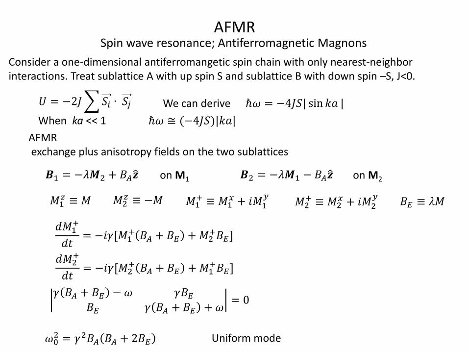
AFMR Spin wave resonance; Antiferromagnetic Magnons
𝑈 = −2𝐽 𝑆𝑖 ∙ 𝑆𝑗 We can derive ℏ𝜔 = −4𝐽𝑆| sin 𝑘𝑎 |
When ka << 1 ℏ𝜔 ≅ (−4𝐽𝑆)|𝑘𝑎|
Consider a one-dimensional antiferromangetic spin chain with only nearest-neighbor interactions. Treat sublattice A with up spin S and sublattice B with down spin –S, J<0.
AFMR exchange plus anisotropy fields on the two sublattices
𝑩1 = −𝜆𝑴2 + 𝐵𝐴𝒛
𝑑𝑀1+
𝑑𝑡= −𝑖𝛾[𝑀1
+ 𝐵𝐴 + 𝐵𝐸 + 𝑀2+𝐵𝐸]
𝑑𝑀2+
𝑑𝑡= −𝑖𝛾[𝑀2
+ 𝐵𝐴 + 𝐵𝐸 + 𝑀1+𝐵𝐸]
𝛾 𝐵𝐴 + 𝐵𝐸 − 𝜔 𝛾𝐵𝐸
𝐵𝐸 𝛾 𝐵𝐴 + 𝐵𝐸 + 𝜔= 0
𝜔02 = 𝛾2𝐵𝐴 𝐵𝐴 + 2𝐵𝐸 Uniform mode
on M1 𝑩2 = −𝜆𝑴1 − 𝐵𝐴𝒛 on M2
𝑀1𝑧 ≡ 𝑀 𝑀2
𝑧 ≡ −𝑀 𝑀1+ ≡ 𝑀1
𝑥 + 𝑖𝑀1𝑦
𝑀2+ ≡ 𝑀2
𝑥 + 𝑖𝑀2𝑦
𝐵𝐸 ≡ 𝜆𝑀
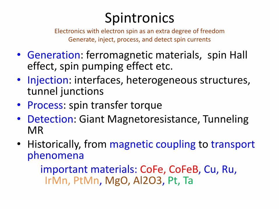
Spintronics Electronics with electron spin as an extra degree of freedom
Generate, inject, process, and detect spin currents
• Generation: ferromagnetic materials, spin Hall effect, spin pumping effect etc.
• Injection: interfaces, heterogeneous structures, tunnel junctions
• Process: spin transfer torque • Detection: Giant Magnetoresistance, Tunneling
MR • Historically, from magnetic coupling to transport
phenomena important materials: CoFe, CoFeB, Cu, Ru, IrMn, PtMn, MgO, Al2O3, Pt, Ta

Magnetic coupling in superlattices • Long-range incommensurate magnetic order in a Dy-Y multilayer M. B. Salamon, Shantanu Sinha, J. J. Rhyne, J. E. Cunningham, Ross W. Erwin, Julie Borchers, and C. P. Flynn, Phys. Rev. Lett. 56, 259 - 262 (1986)
• Observation of a Magnetic Antiphase Domain Structure with Long- Range Order in a Synthetic Gd-Y Superlattice C. F. Majkrzak, J. W. Cable, J. Kwo, M. Hong, D. B. McWhan, Y. Yafet, and J. V.
Waszczak,C. Vettier, Phys. Rev. Lett. 56, 2700 - 2703 (1986)
• Layered Magnetic Structures: Evidence for Antiferromagnetic Coupling of Fe Layers across Cr Interlayers P. Grünberg, R. Schreiber, Y. Pang, M. B. Brodsky, and H. Sowers, Phys. Rev. Lett. 57, 2442 - 2445 (1986)
RKKY (Ruderman-Kittel-Kasuya-Yosida ) interaction
coupling coefficient
38

Magnetic coupling in multilayers
•Long-range incommensurate magnetic order in a Dy-Y multilayer M. B. Salamon, Shantanu Sinha, J. J. Rhyne, J. E. Cunningham, Ross W. Erwin, Julie Borchers, and C. P. Flynn, Phys. Rev. Lett. 56, 259 - 262 (1986)
•Observation of a Magnetic Antiphase Domain Structure with Long- Range Order in a Synthetic Gd-Y Superlattice C. F. Majkrzak, J. W. Cable, J. Kwo, M. Hong, D. B. McWhan, Y. Yafet, and J. V. Waszczak,C.
Vettier, Phys. Rev. Lett. 56, 2700 - 2703 (1986)
•Layered Magnetic Structures: Evidence for Antiferromagnetic Coupling of Fe Layers across Cr Interlayers P. Grünberg, R. Schreiber, Y. Pang, M. B. Brodsky, and H. Sowers, Phys. Rev. Lett. 57, 2442 - 2445 (1986)
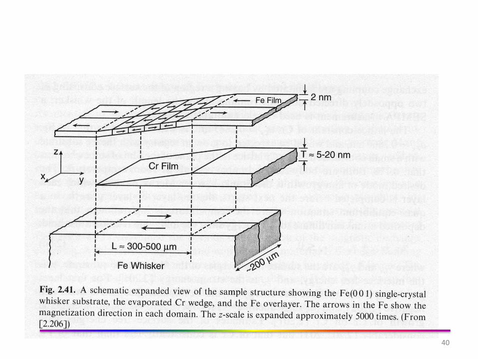
Coupling in wedge-shaped Fe/Cr/Fe
Fe/Au/Fe
Fe/Ag/Fe
J. Unguris, R. J. Celotta, and D. T. Pierce
39
40
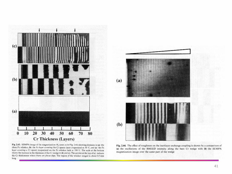
41


Oscillatory magnetic coupling in multilayers
Ru interlayer has the largest coupling strength
43 Kwo et al, PRB 35 7295 (1987) Modulated magnetic properties in synthetic rare-earth Gd-Y superlattices
S. S. P. Parkin
|J1| at 1st peak (erg/cm2)
Period (nm)
Cu 0.3 1
V 0.1 0.9
Cr 0.24 1.8
Ir 0.81 0.9
Ru 5.0 1.2

Spin-dependent conduction in
Ferromagnetic metals (Two-current model)
4
)(
First suggested by Mott (1936)
Experimentally confirmed by I. A. Campbell and A. Fert (~1970)
At low temperature
At high temperature
Spin mixing effect equalizes two currents 44

0.3
20
Ti V Cr Mn Fe Co Ni
= /
10
20
,
(
cm
)
Two Current Model
s electrons carry the electric current
number of empty d states
resistivity (spin-dependent s → d scattering)
A. Fert, I.A. Campbell, PRL 21, 1190 (1968)
spin selective scattering
45
46
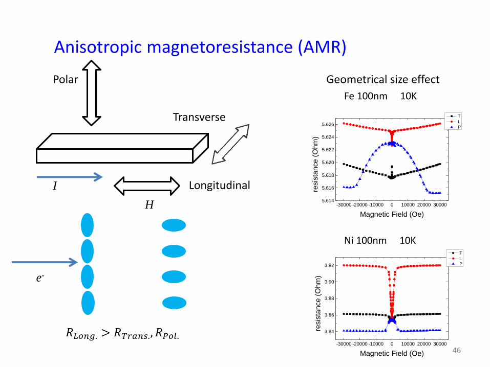
Anisotropic magnetoresistance (AMR)
Polar
Geometrical size effect
Longitudinal
Transverse
I
H
e-
𝑅𝐿𝑜𝑛𝑔. > 𝑅𝑇𝑟𝑎𝑛𝑠., 𝑅𝑃𝑜𝑙.
Ni 100nm 10K
Fe 100nm 10K
-30000 -20000 -10000 0 10000 20000 30000
3.84
3.86
3.88
3.90
3.92
resis
tance (
Ohm
)
Magnetic Field (Oe)
T
L
P
-30000 -20000 -10000 0 10000 20000 300005.614
5.616
5.618
5.620
5.622
5.624
5.626
resis
tance (
Ohm
)
Magnetic Field (Oe)
T
L
P


