Download - MatthieuAussal Research engineer

Fast methods for integral equations
Matthieu AussalResearch engineer
Centre de Mathématiques Appliquées de l’École PolytechniqueRoute de Saclay - 91128 Palaiseau CEDEX France
Journée de rentrée du CMAP - 03 octobre 2018

Introduction
Integral representation
Integral equations
Acceleration
Gypsilab
Conclusion

Main research topics and collaborations
Spatial audio (3D audio) :I VST plug’in for sound engineers (F. Salmon, CNSMDP),I Audio guidance for blind people (S. Ferrand, MCV ),I Classroom sonorization (Mon cartable connecté).
Auralization :I Numerical room acoustics for archeology (R. Gueguen),I Real-time room acoustic for virtual reality,I Augmented reality for museum visit (PSC, MusiX )
Finite and boundary element method (FEM, BEM) :I Gypsilab : Matlab framework for fast prototyping (F. Alouges)I Fast methods for High Performance Computing :
DDM, H-Matrix, FFM, ray-tracing, etc.I Applications (scattering, 3D audio, eeg, Stokes flows, etc.)
Past, present and future collaborations

Some selected softwares
MyBino (freeware) :Professional VST plug’in for
binaural rendering.
Just4rir (open-source) :Blender plug’in for roomacoustics by ray-tracing.
Gypsilab (open-source part) :Matlab framework for fastFEM-BEM prototyping.
Gypsilab (private part) :High-Performance Computing for
FEM-BEM problems.

Introduction
Integral representation
Integral equations
Acceleration
Gypsilab
Conclusion

A boundary problem for acoustic
The full space Ω is separated intwo subspaces Ωi and Ωe by aboundary Γ, smooth and orientedalong normal n.
For u : Ω \ Γ→ C, we define :I ui = u|Ωi
I ue = u|Ωe ,I µ = [u] = ui − ue ,I λ = [∂nu] = ∂nui − ∂nue .
Note : Γ is a singularity of Ω ⇒ Distribution theory !

Theorem of integral representationIf u satisfies Helmholtz equation and Sommerfeld condition :
−(∆ui + k2ui ) = 0 in Ωi ,−(∆ue + k2ue) = 0 in Ωe ,
limr→+∞
r (∂r ue + ikue) = 0,
then u satisfies an integral representation ∀x ∈ Ωi ∪ Ωe :
u(x) =∫
ΓG(x, y)λ(y)dΓy −
∫Γ
∂G(x, y)∂ny
µ(y)dΓy ,
with G(x, y) stand for the oscillatory Green kernel :
G(x, y) = eik|x−y|
4π|x− y| .
Note : Volumic data are fully determined by surfacic unknowns.

Evaluation of boundary integrals
I Regular integration are done using a quadrature rule(yq, γq)1≤q≤Nq for the boundary Γ :
∫Γ
G(x, y)λ(y)dΓy ≈Nq∑
q=1γqG(x, yq)λφ(yq).
I If necessary, singular integrations are done analytically...and it’s hard ! (A. Lefebvre-Lepot)
Note : Regular integration can be seen as a discrete convolutionon a non-uniform grid... meshless technics !

Numerical application
Integral representation of the elementary solution E = − eik|x|
4π|x| .Boundary Γ is a unit sphere, meshed with 2 000 triangles and wavenumber is fixed at k = 5 :
u(x) =∫
Γ G(x, y)∂nE (y)dΓy −∫Γ∂G(x,y)∂ny
E (y)dΓy
Reference E (x), computedanalytically in full space
Introduction
Integral representation
Integral equations
Acceleration
Gypsilab
Conclusion
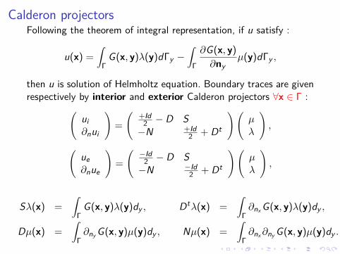
Calderon projectorsFollowing the theorem of integral representation, if u satisfy :
u(x) =∫
ΓG(x, y)λ(y)dΓy −
∫Γ
∂G(x, y)∂ny
µ(y)dΓy ,
then u is solution of Helmholtz equation. Boundary traces are givenrespectively by interior and exterior Calderon projectors ∀x ∈ Γ :(
ui∂nui
)=(
+Id2 − D S−N +Id
2 + Dt
)(µλ
),
(ue∂nue
)=(−Id
2 − D S−N −Id
2 + Dt
)(µλ
),
Sλ(x) =∫
ΓG(x, y)λ(y)dy ,
Dµ(x) =∫
Γ∂ny G(x, y)µ(y)dy ,
Dtλ(x) =∫
Γ∂nx G(x, y)λ(y)dy ,
Nµ(x) =∫
Γ∂nx∂ny G(x, y)µ(y)dy .

Integral formulation : Example with Dirichlet scattering1. Formulate problem considering ue = utot − uinc :
−(∆ue + k2ue) = 0 in Ωe ,lim
r→+∞r (∂r ue + ikue) = 0,utot = 0⇔ ue = −uinc in Γ.
2. Choose the right projector (according to normal n) :(ue∂nue
)=(−Id
2 − D S−N −Id
2 + Dt
)(µλ
).
3. Choose a jump extension :
ui = ue ⇔ µ = 0.
4. Solve integral equation on Γ :
Sλ = ue = −uinc .
5. Compute the total field on Ωe :
utot = Sλ+ uinc .
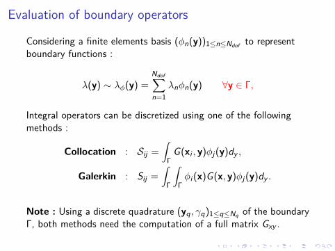
Evaluation of boundary operators
Considering a finite elements basis (φn(y))1≤n≤Ndof to representboundary functions :
λ(y) ∼ λφ(y) =Ndof∑n=1
λnφn(y) ∀y ∈ Γ,
Integral operators can be discretized using one of the followingmethods :
Collocation : Sij =∫
ΓG(xi , y)φj(y)dy ,
Galerkin : Sij =∫
Γ
∫Γφi (x)G(x, y)φj(y)dy .
Note : Using a discrete quadrature (yq, γq)1≤q≤Nq of the boundaryΓ, both methods need the computation of a full matrix Gxy .
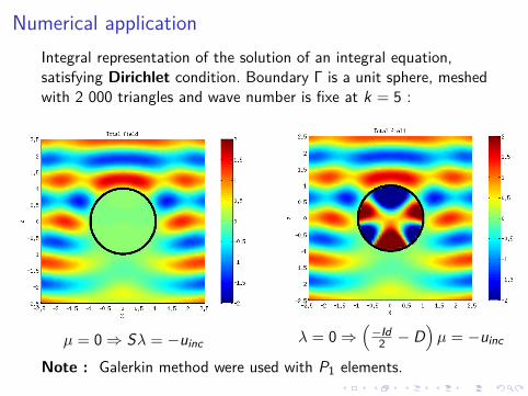
Numerical applicationIntegral representation of the solution of an integral equation,satisfying Dirichlet condition. Boundary Γ is a unit sphere, meshedwith 2 000 triangles and wave number is fixe at k = 5 :
µ = 0⇒ Sλ = −uinc λ = 0⇒(−Id
2 − D)µ = −uinc
Note : Galerkin method were used with P1 elements.

Introduction
Integral representation
Integral equations
Acceleration
Gypsilab
Conclusion

Example with a regular kernel
All integral formulations need discrete convolutions with Greenkernel on non-uniform grids (xi )i∈[1,Nx ] and (yj)j∈[1,Ny ] in R3 :
ui =Ny∑j=1
G(xi , yj)vj .
For example, considering a regular Green kernel :
K (x, y) = |x− y|2 = |x|2 − 2x · y + |y|2,
Convolution by K can be rewritten for all i :
ui = |xi |2Ny∑j=1
vj − 2xi ·Ny∑j=1
yjvj +Ny∑j=1|yj |2vj
Separate x and y : Complexity O(NxNy )→ O(Ny ) + O(Nx) !

Example with a singular kernel
Context : G(x, y) = eik|x−y|
4π|x−y| is locally singular (|x− y| < ε).
Idea : Use "smoothing" properties issued from far distances.
Method : Divide and conquer with distance criterion.
Algorithm(s) : Hierarchical tree and leaves compression.
Initialization : Considering a space sampling (xi )i∈[1,Nx ] and(yj)j∈[1,Ny ] in R3, a Green kernel matrix is given by :
Gxy =
G(x1, y1) ... G(x1, yNy )... ... ...
G(xNx , y1) ... G(xNx , yNy )
= [G0]
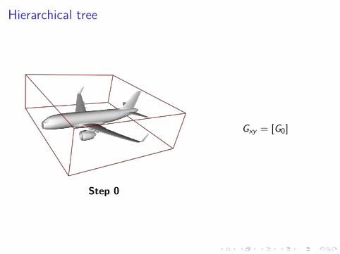
Hierarchical tree
Step 0
Gxy = [G0]

Hierarchical tree
Step 1
Gxy =[
G1 G2G3 G4
]
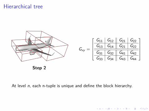
Hierarchical tree
Step 2
Gxy =
G11 G12 G21 G22G13 G14 G21 G22
G31 G32 G41 G42G33 G34 G43 G44
At level n, each n-tuple is unique and define the block hierarchy.

Hierarchical tree
Step 3
Gxy =
G111 G112 ... G221 G222G113 G114 ... G223 G224
... ... ... ... ...
G331 G332 ... G441 G442G333 G334 ... G444 G444
Green leaves are far away ⇒ no recursion.

Hierarchical tree
Step 4

Hierarchical tree
Step 5

Hierarchical tree
Step 6
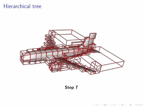
Hierarchical tree
Step 7

Hierarchical tree
and finally ...

Hierarchical tree
The last level is reached !
Green cells → far interactionsRed cells → close interactions

Leaves compression
Idea : Use "smoothing" properties issued from far distances tointerpolate interactions → data compression !
Method : Considering Gij = (G(xi , yj))i∈I,j∈J a block of farinteractions, indexed by I ∈ [1,Nx ] and J ∈ [1,Ny ] :I Weak interpolation :
G(x, y) =∑
kIk(x, ξk)G(ξk , y) ⇒ GIJ = AIkBkJ .
I Strong interpolation :
G(xi , yj) =∑k,lIk(x, ξk)G(ξk , ξl )Il (ξl , y) ⇒ GIJ = AIkTklBlJ .

Final matrix formFull Weak Strong

Non exhaustive list of fast solvers
Method Class Interpolation Complexity AlgebraFull - - N2 (yes)
H1-matrix weak SVD/ACA N3/2 yesH2-matrix strong Lagrange N log N yes/noSCSD strong Cardinal sine N6/5 no
FMM/FFM strong Plane wave N log N no
I SVD/ACA : G = ABt with A and B low-rank matrices,I Lagrange : G = A ∗ T ∗ Bt , A and B low-rank and T small,I Plane wave :
G(x, y) = ik16π2 limL→+∞
∫s∈S2 eiks·xM1T L
M1M2(s)eiks·M2yds
I Cardinal sine :G(x, y) = k
(4π)2∑+∞
n=0 αnρn∫
S2 eikρns·xe−ikρns·yds

Numerical application
Context : For all particles (xi )i∈[1,N] and (yj)j∈[1,N] in R3 :
u(xi ) =N∑
j=1
14π|xi − yj |
v(yj),
⇔ U = M ∗ V .
with M ∈ MN(R), U and V ∈ RN .
Test case : (xi )i∈[1,N] and (yj)j∈[1,N] are uniformly distributed onthe unit sphere S2.
Computer : 12 core at 2.7 GHz, 256 GO de ram, Matlab R2014a.

Numerical Application
N Time (s) Memory peak
104 2.04 1 Mo105 328 10 Mo
Full product (single thread)
N Build time (s) MV time (s) LU time (s) Mem104 8.24 0.16 9.88 100 Mo105 78.9 1.68 145 1 Go106 1069 25 4120 10 Go
H1-matrix product and algebra with ε = 10−3 (single-thread)

Numerical Application
N Time 1 core (s) Time 12 cores (s) Error L2 Mem
104 2.04 9.08 8.03 10−5 1 Mo105 9.30 17.1 1.34 10−4 10 Mo106 87.8 33.4 1.35 10−4 100 Mo107 1063 169 1.98 10−4 1 Go108 - 1499 1.81 10−4 10 Go109 - 11340 3.11 10−4 100 Go
Fast and Furious product with ε = 10−3 (multi-thread)
Note : Assembly, full matrix would weigh 8 exa-octets !(double precision : 8N2 → 8 1018 Bytes)

Introduction
Integral representation
Integral equations
Acceleration
Gypsilab
Conclusion


But what is Gypsilab ?Gypsilab is an open-source framework for Matlab, freelyavailable under GPL 3.0, composed of object-oriented libraries :I openMsh : Multi-dimensional mesh management.
I openDom : Numerical integration and variational calculation,joint work with François Alouges.
I openFem : Finite Element method for 2D and 3D shapes,joint work with François Alouges.
I openHmx : H-Matrix compression and algebra.
I openRay : Accelerated ray-tracing for HF problems,joint work with Robin Gueguen.
Designed to combine industrial requirements with fastprototyping.

Licensed add-on for Gypsilab
Open source part of Gypsilab is accompanied by licensedadd-on, also composed of object-oriented libraries :
I libHbm : Block matrix computation and algebra.Domain Decomposition Method, H-Matrix Parallelization,multi-physic coupling, out-of core computation, etc.
I libFfm : Fast and Furious Method.High Performance Computing for very large BEM problems.

Application 1 : Head-Related Tranfert Function (3D audio)
Helmholtz equation
Neumann boundary condition
P1 finite element
10−3 compression accuracy
50.000 dof at 8 kHz
H-Matrix exact solver
Figure – Acoustic scatering by humanhead, mesh from SYMARE database.

Application 2 : Radar detection (ISAE 2016)Maxwell equationPEC boundary condition, CFIERWG finite element
10−3 compression accuracy300.000 dof at 2.5 GHzH-Matrix exact solver
Figure – Electromagnetic scattering by an UAV, workshop ISAE, meshfrom Onera.

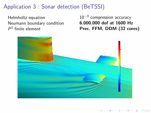
Application 3 : Sonar detection (BeTSSI)
Helmholtz equationNeumann boundary conditionP1 finite element
10−3 compression accuracy6.000.000 dof at 1600 HzPrec. FFM, DDM (32 cores)
Application 3 : Sonar detection (BeTSSI)
Helmholtz equationNeumann boundary conditionP1 finite element
10−3 compression accuracy6.000.000 dof at 1600 HzPrec. FFM, DDM (32 cores)

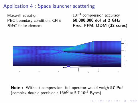
Application 4 : Space launcher scatteringMaxwell equationPEC boundary condition, CFIERWG finite element
10−3 compression accuracy60.000.000 dof at 2 GHzPrec. FFM, DDM (32 cores)
Note : Without compression, full operator would weigh 57 Po !(complex double precision : 16N2 ≈ 5.7 1016 Bytes)
Application 4 : Space launcher scatteringMaxwell equationPEC boundary condition, CFIERWG finite element
10−3 compression accuracy60.000.000 dof at 2 GHzPrec. FFM, DDM (32 cores)
Note : Without compression, full operator would weigh 57 Po !(complex double precision : 16N2 ≈ 5.7 1016 Bytes)

Application 4 : Space launcher scatteringMaxwell equationPEC boundary condition, CFIERWG finite element
10−3 compression accuracy60.000.000 dof at 2 GHzPrec. FFM, DDM (32 cores)
Note : Without compression, full operator would weigh 57 Po !(complex double precision : 16N2 ≈ 5.7 1016 Bytes)

Introduction
Integral representation
Integral equations
Acceleration
Gypsilab
Conclusion

ConclusionI CommunicationsI Kalman filterring with H-Matrix (P. Moireau)I Electro-encephalogram with H-Matrix (A. Gramfort et al)I Vibro-acoustic with FFM (Naval group)I Add numericals methods (Finite volume, finite difference, etc).I Mesh generation (2D, 3D, coupling)I Reach world’s records (3.109 Maxwell, 70.109 Stokes)
Download gypsilab : www.cmap.polytechnique.fr/~aussal
Il faut se débarrasser des casse-têtes.On ne vit qu’une fois.
Charles Aznavour, 1924-2018


