DPRIETI Discussion Paper Series 12-E-062
Natural Disasters, Damage to Banks, and Firm Investment
HOSONO KaoruGakushuin University
UCHINO TaisukeRIETI
ONO AritoMizuho Research Institute
UESUGI IichiroRIETI
MIYAKAWA DaisukeDevelopment Bank of Japan
HAZAMA MakotoHitotsubashi University
UCHIDA HirofumiKobe University
The Research Institute of Economy, Trade and Industryhttp://www.rieti.go.jp/en/
1
RIETI Discussion Paper Series 12-E-062
October 2012
Natural Disasters, Damage to Banks, and Firm Investment
HOSONO Kaoru (Gakushuin University / Ministry of Finance)
MIYAKAWA Daisuke (Development Bank of Japan-RICF)
UCHINO Taisuke (Daito Bunka University / RIETI)
HAZAMA Makoto (Hitotsubashi University)
ONO Arito (Mizuho Research Institute)
UCHIDA Hirofumi (Kobe University)
UESUGI Iichiro (Hitotsubashi University / RIETI)
Abstract
This paper investigates the effect of banks’ lending capacity on firms’ capital investment. To
overcome the difficulties in identifying purely exogenous shocks to firms’ bank financing, we utilize
the natural experiment provided by the Great Hanshin-Awaji (Kobe) Earthquake in 1995. Using a
unique firm-level dataset that allows us to identify firms and banks in the earthquake-affected area,
together with information on bank-firm relationships, we find that the investment ratio of firms
located outside of the earthquake-affected area but with their main banks inside the area was lower
than that of firms that were both located and had their main banks outside of the area. This result
implies that the weakened lending capacity of damaged banks exacerbated the borrowing constraints
on the investment of their undamaged client firms. We also find that the negative impact is robust for
two alternative measures of bank damage: that to the bank headquarters and that to the branch
network. However, the impacts of the two are different in timing; while that of the former emerged
immediately after the earthquake, the latter emerged with a one-year lag.
Keywords: Natural disasters; Bank damage; Lender bank; Capital investment.
JEL classification: E22, G21, G3
This paper is a product of the Study group for Earthquake and Enterprise Dynamics (SEEDs), which participates in the
project "Design of Interfirm Networks to Achieve Sustainable Economic Growth" under the program for Promoting Social
Science Research Aimed at Solutions of Near-Future Problems conducted by the Japan Society for the Promotion of
Science (JSPS), the earthquake study project at the Research Institute of Economy, Trade and Industry (RIETI), and the
academic investigation project into the Great East Japan Earthquake by the JSPS. We are thankful for financial support
from Hitotsubashi University and for the data provided by Teikoku Databank, Ltd. K. Hosono gratefully acknowledges
financial support from Grant-in-Aid for Scientific Research (B) No. 22330098, JSPS, and H. Uchida acknowledges support
from Grant-in-Aid for Scientific Research (B) No. 24330103, JSPS.
RIETI Discussion Papers Series aims at widely disseminating research results in the form of professional papers, thereby stimulating lively discussion. The views expressed in the papers are solely those of the author(s), and do not represent those of the Research Institute of Economy, Trade and Industry.

1
1. Introduction
Does the lending capacity of banks affect the activities of firms that borrow from those banks?
A vast literature has tried to answer this question since the seminal work by Bernanke (1983). However,
researchers are faced with an identification problem: while lending behavior affects borrowing firms’
performance, the performance of borrowing firms itself has a significant impact on the way lenders
extend loans. This paper tackles this problem by taking advantage of the natural experiment provided by a
natural disaster, which allows us to single out a purely exogenous shock to firms’ bank financing.
A natural disaster may obliterate information on borrowers’ creditworthiness accumulated by the
disaster-hit banks, and thus destroy their managerial capacity to originate loans, including the ability to
screen and process loan applications. A natural disaster may also cause damage to borrowing firms
located in the neighborhood of such banks, leading to deterioration in the banks’ loan portfolios and
risk-taking capacity. In either case, a disaster reduces the damaged banks’ lending capacity. Thus, for
those firms that are not directly damaged by the disaster, damage to banks that they borrow from is an
exogenous shock that may affect the availability and the cost of external funds they can access. A natural
disaster thus provides us a good laboratory for studying the effect of banks’ lending capacity on
borrowing firms’ investment.
To that end, this paper focuses on the Great Hanshin-Awaji (Kobe) Earthquake, which hit the
area around Kobe City and Awaji Island in western Japan in January 1995. We examine whether damage
to banks had an adverse impact on the investment of client firms that did not themselves suffer any
damage. To do so, we construct and use a unique firm-level dataset compiled from various sources. The
dataset includes information on firms’ main banks,1 on their investment levels, and on whether these
banks and firms were located inside or outside the earthquake-affected area. The dataset also includes
information from firms’ and banks’ financial statements. Thus, our sample consists of four groups of
firm-bank pairs: damaged/undamaged firms, paired with damaged/undamaged banks. By comparing
undamaged firm-damaged bank pairs with undamaged firm-undamaged bank pairs, we are able to single
out the effect of damage to banks on the investment of undamaged firms.
Our main findings can be summarized as follows. First, firms located outside the
earthquake-affected area but associated with a main bank located inside the area had a lower investment
ratio than outside firms associated with a main bank located outside the area. This result implies that the
exogenous damage to banks’ lending capacity had a significant adverse effect on firm investment. Second,
1 Our dataset includes information on the banks that firms transact with. Among those banks, we treat the bank that a firm regards as the “most important” as the firm’s main bank. See Section 5 for more details.

2
the finding above is robust to two alternative measures of bank damage: A) damage to a bank’s
headquarters, which captures the decline in a bank’s managerial capacity to process loan applications at
the back office, and B) damage to a bank’s branch network, which captures the decline in a bank’s
financial health and risk-taking capacity. Our results imply that both of these transmission mechanisms
were important. However, we also find that the impact of headquarters damage emerged immediately
after the earthquake, while the impact of branch damage appeared only with a one-year lag.
The contributions of this paper to the literature are twofold.2 First, by using a natural experiment,
we are able to circumvent the identification problem faced by many existing studies on the effects of bank
lending on firm activities – namely, the difficulty in distinguishing between a loan supply shock and a
loan demand shock. Our matched firm-bank data also allow us to identify the mechanism through which
the lending capacity of banks affects the activities of borrowing firms in a more precise manner than
many other studies that are based on aggregate data (e.g., Peek and Rosengren 2000). Second, this paper
is closely related to the literature that investigates the effects of natural disasters on corporate activities.
Many of these studies use country or regional level data and thus are unable to clarify the effects of
disasters on individual firms. Leiter et al. (2009) and De Mel et al. (2010) examine the recovery of
disaster-hit firms using a firm level dataset, but our uniqueness rests on the fact that we investigate the
negative impact of damage to banks not only on earthquake-hit firms but also on undamaged firms as
well.
The rest of the paper is structured as follows. Section 2 reviews the related literature and our
contribution in greater detail. Section 3 provides a brief overview of the Kobe earthquake. Sections 4 and
5 describe our data and methodology, respectively, and Section 6 reports our results. Section 7
summarizes the results and concludes.
2. Literature Review
2.1 Bank Loans and Firm Activities
There is a vast literature that examines empirically the effects of bank lending on the real economy.
In his seminal paper, Bernanke (1983), using aggregate data, purported to show that bank failures
significantly reduced aggregate production in the US economy during the Great Depression. His study,
however, has been challenged on the grounds that it does not identify loan supply shocks as distinct from
shocks to loan demand. In other words, the observed relationship between bank failures and aggregate
2 See Section 2 for more details.

3
production may simply capture the fact that the recession caused bank failures. In fact, using US
state-level data for the 1990-91 recession, Bernanke and Lown (1991) find no significant relationship
between bank lending and employment growth when the loan growth is instrumented for by the bank
capital-asset ratio, suggesting that a credit crunch was not a major cause of the 1990-91 recession.
There are some event studies examining the effect of bank failures on the market values of their
client firms. Slovin et al. (1993) are the first to analyze the stock prices of firms that had lending
relationships with the Continental Illionis Bank during the period of its de facto failure. This study is
followed by Yamori and Murakami (1999), Bae et al. (2002), and Brewer et al. (2003a), all of which find
a significant effect of bank failures on the market values of firms that borrow from those banks.3
Similarly, Yamori (1999) investigates the failure of a regional bank in Japan (Hyogo Bank), and finds that
the subsequent returns on the stocks of the problem banks were significantly lower than those of solvent
banks.4 The advantage of these event studies is that they are able to clearly identify bank failure shocks
using high-frequency (daily) data. However, they have limitations as well. First, event studies rely on the
assumptions of market efficiency and rational investor behavior. Second, event studies cannot be applied
to non-listed firms. In this paper we focus on a real activity of firms, i.e., investment behavior, and hence
do not require any assumptions of market efficiency or rationality. In addition, we analyze unlisted firms,
most of which are small and medium-sized and therefore likely to be severely affected by shocks from
lending banks.
Several other studies use firms’ financial statements to investigate the effects of bank failures or
weak bank health on client firms.5 For instance, Hori (2005) examines the profitability of firms that
borrowed from a large failed Japanese bank (Hokkaido-Takushoku Bank), and finds adverse effects on
firms with low credit ratings. Similarly, Minamihashi (2011) analyzes the failures of two long-term credit
banks in Japan, and finds that the failures significantly decreased the investment of their client firms.6
Finally, Gibson (1995, 1997) finds that client firms that were borrowing from Japanese banks with low
credit ratings significantly reduced their investment during 1994-95.7 However, these studies suffer from
the aforementioned identification problem, because the direction of the causality between bank failure (or
3 Note, however, that Brewer et al. (2003a) also find that the magnitude of these negative effects on the values of borrower firms is not significantly different from that on all other firms in their sample. 4 See also Brewer et al. (2003b). 5 Using bank balance sheet data, Woo (2003) and Watanabe (2007) find that weakly capitalized Japanese banks reduced their lending in 1997, when the Ministry of Finance started to impose rigorous self-assessments of loan classifications. 6 See also Fukuda and Koibuchi (2007). 7 See also Nagahata and Sekine (2005). Using data of listed Japanese firms for the period 1993-1999, Peek and Rosengren (2005) find that banks expanded loans to unprofitable firms during this period. See also Caballero et al. (2008) for such “zombie” lending practices by Japanese banks in the 1990s.

4
weak bank health) and client firms’ poor performance is unclear.
To resolve that identification problem, Peek and Rosengren (2000) examine whether state-level
construction activities in the United States were affected by the deterioration in the health of Japanese
banks, through reductions in those banks’ lending at their US branches. They find that the firms were
indeed affected, with clearly identified causality running from bank lending capacity to firm activities.
The identification strategy employed in this paper is similar to the one employed in that paper, since we
examine the effect of damage to banks on firms that are located outside the earthquake-hit area. However,
Peek and Rosengren (2000) use state-level aggregate data, so they cannot control for firm and bank
heterogeneity. We have the advantage of being able to more clearly capture the effects of the damage to
lending banks, because we use firm- and bank-level data.
The papers most closely related to the present study are Khwaja and Mian (2008) and Berg and
Schrader (2012). Khawaji and Mian (2008) examine the transmission of a bank liquidity shock to client
firms’ financial distress in an emerging market (Pakistan), while Berg and Schrader (2012) analyze the
effects of volcanic eruptions on borrowing from a microfinance institution in a developing economy
(Ecuador). In this paper we show that a shock to bank lending capacity affects client firms’ activity even
in an economy with well-developed financial markets and institutions.
Finally, there is also an emerging strand of literature that examines the international transmission
of financial crises. Chava and Purnanandam (2011) and Schnabl (2012) use the 1998 Russian sovereign
default as a bank liquidity shock, and examine its international transmission to both the US and to an
emerging market (Peru). Popov and Udell (2010) examine the cross-border transmission of the 2008-09
financial crisis from West European and U.S. banks to firms in Central and Eastern Europe. Paravisini et
al. (2011) study the impact of the capital flow reversals during the 2008 financial crisis on Peruvian firms.
Cetorelli and Goldberg (2012) investigate lending by the U.S. branches of foreign banks during the Great
Recession. We differ from these studies in that we focus on the domestic transmission of a shock from
banks in disaster-hit areas to their client firms in other areas.
2.2 Natural Disasters and Economic Recovery
This paper is also related to the literature on the economic consequences of, and recovery from,
major natural disaster events. Natural disasters cost lives and destroy infrastructure, buildings, and
machinery, and thereby affect both labor and capital. They also not only disrupt the business operations of
firms directly affected by the disaster, but also impact the operations of non-affected firms through

5
upstream and downstream supply linkages. However, destroyed capital is typically replaced, and firms’
output and productivity may eventually recover. Although the empirical findings are mixed, cross-country
studies on the factors determining the extent of economic recovery following a major disaster generally
suggest that updating of technology and/or of the composition of production factors, as well as factor
accumulation, play a role (Skidmore and Toya 2002, Okuyama 2003, Kahn 2005, Stromberg 2007, Toya
and Skidmore 2007, Crespo-Cuaresma et al. 2008, Sawada et al. 2011).
However, compared with the rich literature on the macroeconomic impact of natural disasters,
studies exploring the firm-level impact of, and subsequent recovery from, natural disasters are relatively
scarce. Notable exceptions are Leiter et al. (2009) and De Mel et al. (2010). Leiter et al. (2009) examine
the capital accumulation, employment, and productivity growth of European firms affected by floods, and
find that employment growth and accumulation of physical capital are significantly higher in regions
experiencing major flood events. They also find that the positive effect is stronger for firms with a higher
share of intangible assets. De Mel et al. (2010) conduct a series of surveys of enterprises in Sri Lanka
following the 2004 tsunami and examine their recovery from the disaster. In their field experiments, they
randomly provide grants to selected enterprises and investigate the impact of the grants on the firms’
recovery. They find that direct aid had a significant positive impact on the profits of tsunami-affected
enterprises in the retail industry, but not in the manufacturing industry. However, they do not investigate
the role of borrowing from banks, which are major providers of funds. The uniqueness of our study lies in
the fact that we investigate the impact that damage to banks has on non-affected as well as affected
borrowers.8
3. Summary of the Kobe Earthquake
The Kobe earthquake occurred on January 17, 1995. The total loss from this major natural disaster
is estimated to have been 9.9 trillion yen, including 630 billion yen in business sector losses.9 Table 1
provides an overview of the estimated damage, including the number of casualties and the number of
housing units destroyed. There were more than 6,000 casualties, and about 100,000 housing units were
completely destroyed. There is considerable variation in the number of casualties and the extent of
damage across municipalities in the earthquake-affected area.10 The ratio of the number of casualties to
the total population and the ratios of the number of completely and partly destroyed housing units to the
8 Sawada and Shimizutani (2008) focus on financial constraints of households affected by the Kobe earthquake. Their findings suggest that borrowing constraints played an important role in the wake of the disaster. 9 Data provided by Hyogo Prefecture (http://web.pref.hyogo.jp/wd33/wd33_000000010.html). 10 For the exact definition of the “earthquake-affected area,” see section 4.2.

6
total number of housing units are especially high in specific areas of Kobe City, including its wards of
Higashinada, Nada, and Nagata.11
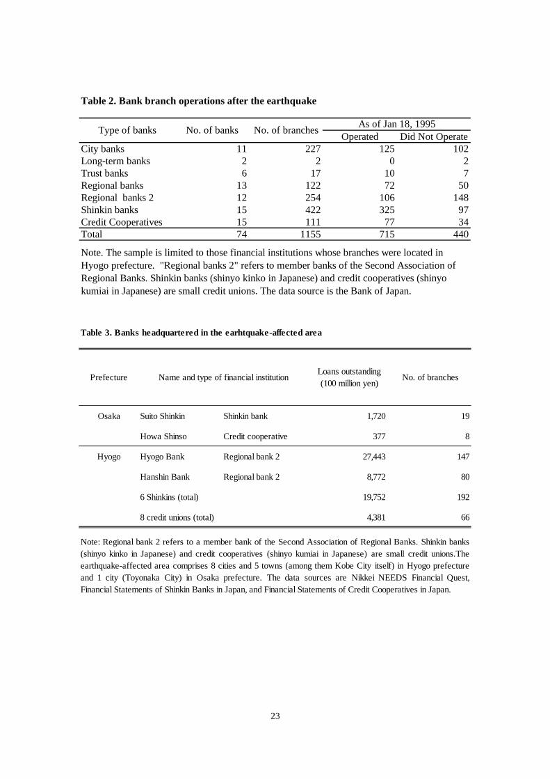
The Kobe earthquake had a serious impact on banks’ operations as well. Table 2 shows that about
a quarter of the bank branches located in Hyogo Prefecture were unable to operate immediately after the
earthquake. Although information is not available regarding how long such disruption of banking
operations continued, Table 3 provides an overview of banks headquartered in the earthquake-affected
area at the time of the earthquake. It shows that 18 banks, including 2 relatively large regional banks,
were directly affected by the disaster. We examine how such bank damage affected borrowing firms’
investment below.
4. Data
4.1 Data sources
We rely primarily on two firm-level data sources. First, information on firms’ capital investment
and financial conditions is obtained from the Basic Survey of Business Structure and Activities (BSBSA;
Kigyo Katsudou Kihon Chosa in Japanese) compiled by the Ministry of Economy, Trade and Industry.
The main purpose of this survey is to gauge quantitatively the activities of Japanese enterprises, including
capital investment, exports, foreign direct investment, and investment in research and development. To
this end, the survey covers the universe of enterprises in Japan with more than 50 employees and with
paid-up capital of over 30 million yen. From this data source, we obtain firm-level data on capital
investment and capital stocks.
Second, we rely on the firm-level database provided by Teikoku Databank LTD. (TDB), a leading
business credit bureau in Japan. In addition to information on firm characteristics, the TDB database
provides a list of the banks with which each firm transacts, where firms rank the banks in the order of
importance to them. We define the bank at the top of each firm’s list as that firm’s main bank. We further
augment our dataset with data from the financial statements of all the main banks, obtained from the
Nikkei NEEDS Financial Quest compiled by Nikkei, Inc. (Nihon Keizai Shimbunsha) and two other,
11 The ratios of completely destroyed, partly destroyed, and completely or partly destroyed housing units in the table should be treated with a degree of caution, because the Fire Defense Agency and the Ministry of Construction (Housing and Land Survey) use slightly different definitions. For example, the ratio of completely or partly destroyed housing units in Nagata-ku is more than 90%, which seems excessively high. For a limited number of cities and towns, we can use alternative survey data collected by the Architectural Institute of Japan, which cover around 80% of the housing in Japan. If we use these data, the ratios of completely, partly, and completely or partly destroyed housing units for Nagata-ku are 25.6%, 22.0%, and 47.6%, respectively.12 These two sources are the “Financial Statements of Shinkin Banks in Japan” and the “Financial Statements of Credit Cooperatives in Japan,” edited by Financial Book Consultants, Ltd. (Kinyu Tosho Konsarutantosha).
7
paper-based sources.12 This augmented dataset is then merged with the first data set from the BSBSA
firm names and addresses.
4.2 Sample Selection
We treat firms whose headquarters are located in the earthquake-affected area as “damaged firms”
(treatment group). The earthquake-affected area is defined as the nine cities and five towns in Hyogo and
Osaka prefectures that were included in the Japanese Government’s Act Concerning Special Financial
Support to Deal with a Designated Disaster of Extreme Severity.13 We choose firms located in Hyogo and
Osaka prefectures as the control group in order to eliminate differences in unobserved characteristics
stemming from region-specific factors. The BSBSA database contains the information of 3897 firms
headquartered in Hyogo and Osaka prefectures, 641 of which were located in the affected area and 3256
in the non-affected area. However, when we merge the Teikoku Databank data with the BSBSA data the
number of firms is reduced to 3,212, of which 591 firms were headquartered in the affected area and
2,621 firms in the non-affected area.
We aim to trace the changes over time in the effects of damages to banks and firms on firms’
investment. To this end, we need a balanced panel dataset that contains the same firms over the
observation period. Therefore, we restrict our sample to firms that do not exit from the sample over our
observation period, i.e., the three years following the earthquake. Although this restriction may raise
concerns about survivor bias, we argue that it does not cause serious problems. Somewhat surprisingly,
the number of firms in the affected area that exited from the sample is not large compared with the
equivalent number in the non-affected area. Table 4 shows the cumulative number of firms who dropped
out of the TDB-BSBSA merged dataset as a proportion of the total number of firms that existed in the
dataset in fiscal year (FY) 1994.14 The drop-out rate in the affected area was actually lower than that in
the non-affected area in FYs 1995 and 1996, though the former was slightly higher than the latter in FY
1997.
We also restrict our sample of firms to those whose main bank survived over the three years after
12 These two sources are the “Financial Statements of Shinkin Banks in Japan” and the “Financial Statements of Credit Cooperatives in Japan,” edited by Financial Book Consultants, Ltd. (Kinyu Tosho Konsarutantosha). 13 The nine cities and five towns consist of Toyonaka City, Kobe City, Amagasaki City, Nishinomiya City, Ashiya City, Itami City, Takarazuka City, Kawanishi City, Akashi City, Tsuna Town, Hokutan Town, Ichinomiya Town, Goshiki Town, and Higashiura Town. Goshiki Town later merged with Sumoto City, and Tsuna, Hokutan, Ichinomiya, and Higashiura towns merged to form Awaji City. 14 The financial year for most firms in Japan is the same as the fiscal year, starting in April and ending in March. For example, FY1995 starts in April 1995 and ends in March 1996. The Kobe Earthquake on January 17, 1995 is thus included in FY1994.

8
the earthquake. Among the banks headquartered in the affected area, we have one bank that failed during
the three year window (Hyogo Bank, which failed in August 1995). A reported reason for the failure was
the expansion of real estate-related loans during the 1980s, which became non-performing when the
Japanese land price bubble burst in the early 1990s. Because we exclude those firms whose main bank
was Hyogo Bank, we can rule out the possibility of a “sick bank” effect. With this exclusion, the number
of firms falls to 2,086, of which 390 were headquartered in the affected area and 1,696 in the non-affected
area.
Finally, to exclude outliers, we drop observations for which our dependent variable or one of the
independent variables (explained below) falls in either of the 0.5% tails of its distribution for the
observation years. The observation period is the three fiscal years following the earthquake (i.e., t =
FY1995, FY1996, and FY1997). Our final dataset consists of 351 damaged firms and 1,604 undamaged
firms. These 1955 firms make up our sample for the empirical analysis in the following sections.15
To see whether our choice of control group and sample selection cause any bias by shifting the
industrial composition of the sample, we compare the industrial composition between damaged firms and
undamaged firms in FY 1995 (Table 5). Though the share of wholesalers is smaller and the share of
retailers and restaurants is larger in the affected area than in the unaffected area, the share of each of the
other industries is almost the same. Importantly, the shares of construction firms, which may have a
strong incentive to invest to meet the demand of public investment following the disaster, are almost the
same between the affected and unaffected areas.
5. Methodology and Variables
5.1 Regression
We estimate the following equation:
)1(.1997,1996,1995,___*_
___
716
1,54
321101
=+++
++
+++=
−
−
−−
tforIndustryCAPACITYBSCONSTRAINTFDAMAGEDBDAMAGEDF
DAMAGEDBDAMAGEDFHSALESGROWTFKI
itiit
tiii
iiitit
it
εββ
ββ
ββββ
This is a Tobin’s Q-type investment equation, which is augmented by a dummy variable
indicating whether the firm is located in the earthquake-affected area, a proxy for bank damage, and
15 The sample size slightly varies over the three year period since we drop outliers for each year.

9
proxies for the firm’s financial constraints and the bank’s lending capacity.
The dependent variable is the capital investment ratio, which is defined as the ratio of
investment during period t to the capital stock at the end of period t-1. This ratio is widely used in existing
empirical studies on investment based on the Q thoery. Taking into account the possibility that the effects
of the earthquake on investment change over time, we run a separate cross-sectional regression for each
fiscal year.
5.2 Explanatory Variables
As regressors, we use a proxy for Tobin’s Q and a variety of additional variables that may affect
investment. For all time-varying variables, we use a one-year lag to eliminate possible endogeneity
problems.
5.2.1 Proxy for Tobin’s Q
Since most of our sample firms are not listed on stock exchanges, we cannot use Tobin’s Q
(defined as the ratio of the market value to the replacement cost of capital) as a regressor to represent
firm’s degree of investment opportunity. We thus follow studies such as Shin and Stulz (1998), Whited
(2006), and Acharya et al. (2007), and instead use the growth rate of firms’ sales (F_SALESGROWTH) as
a proxy for their investment opportunity. F_SALESGROWTH is hypothesized to have a positive
coefficient.
5.2.2 Damaged firm dummy
Because we do not know whether and to what extent each firm actually suffered from the earthquake,
we assume that firms in the affected area are all damaged firms. We use F_DAMAGED, which takes a
value of one if the firm is located in the earthquake-affected area as defined above. Having probably lost
part or all of their physical capital, damaged firms are likely to have a large marginal product of capital,
so that such firms should have greater demand for capital than undamaged firms. We thus predict that this
variable has a positive impact on the investment ratio.
5.2.3 Damaged bank variables
Our main interest lies in the effects of bank damage on borrowing firms’ investment.
B_DAMAGED indicates the damage to a firm’s main bank. Because we have no precise information
10
concerning whether and to what extent banks suffered from the earthquake, we use two alternative
variables for B_DAMAGED. The first alternative is B_HQDAMAGED, a dummy variable that takes a
value of one if the headquarters of the bank are located in the earthquake-affected area. This variable
captures whether the managerial capacity to process loans is impaired; this managerial capacity includes
back-office operations, such as the ability to process applications for large loans or to manage the total
risk of the bank’s loan portfolio.
The second alternative is B_BRDAMAGED, which is the share of the main bank’s branches
located in the earthquake-affected area as a fraction of the total number of branches. Compared to
B_HQDAMAGED, this variable measures the extent of damage to the main bank’s branch network. It
represents the impairment of the main bank’s ability to process applications for relatively small loans
under the authority of branch managers. It also captures the extent of the main banks’ exposure to
damaged and possibly non-performing borrowers, which is likely to negatively affect their risk-taking
capacity. We hypothesize that either of these measures of bank damage imposes borrowing constraints on
client firms, and thus will take a negative coefficient in the regression.
Note that we use the main bank at the time the earthquake occurred (i.e. in FY 1994). This is done
in order to properly identify an exogenous shock to the firm, i.e., whether the firm’s main bank at the time
of the earthquake sustained damage or not. If firms can easily switch their main banks, they might be able
to escape collateral damage from the adverse effects suffered by their earthquake-affected main banks;
this would reduce the size of the coefficients on B_HQDAMAGED and B_BRDAMAGED. However, we
find that firms in our sample rarely changed their main banks. As shown in Table 6, only 5.9% of all
firms, and only 7.7% of the firms in the affected area, switched their main banks during the three years
following the earthquake.
5.2.4 Interaction of damaged firms and damaged banks
In addition to F_DAMAGED and B_DAMAGED, we also add a term interacting these two
variables. This is done to differentiate the impact of bank damage on damaged firms from that on
undamaged firms. As mentioned earlier, what we are most interested in is the effect of bank damage on
undamaged borrowers, which is captured by the coefficient on B_DAMAGED. On the other hand, the
effect of bank damage on damaged borrowers is captured by the sum of the coefficients on B_DAMAGED
and on the interaction term of B_DAMAGED and F_DAMAGED. If bank damage has a negative impact
on damaged borrowers, the sum of these coefficients will take a negative value.
11
5.2.5 Firms’ financial constraints
We also include a vector of variables representing firms’ financial constraints, F_CONSTRAINTS.
Specifically, we use firms’ size, which is represented by the natural logarithm of total assets
(F_LNASSETS); their leverage, which is computed as the ratio of total liabilities to total assets (F_LEV);
their profitability, which is represented by the ratio of current income to total assets (F_ROA); and their
liquidity, which is proxied for by the ratio of liquid assets to total assets (F_CASH).
Recent studies, including Whited (2006), Bayer (2006), and Hennessy et al. (2007), consider
financial frictions to be important factor generating variations in firm investment. Firms with higher
profitability (F_ROA), more liquidity (F_CASH), and larger size (F_LNASSET) are less likely to be
financially constrained. Note, however, that these firm characteristics could be also related to future
profitability, as discussed by Abel and Eberly (2011) and Gomes (2001). But regardless of which
interpretation is correct, we expect the coefficients on these variables to be positive. On the other hand,
since firms with higher leverage (F_LEV) are more likely to be financially constrained, we expect F_LEV
to have a negative coefficient.
5.2.6 Banks’ lending capacity
Finally, we include a vector of variables representing the main bank’s lending capacity,
B_CAPACITY. More specifically, we control for the size, financial health, and profitability of each firm’s
main bank. For size, we use the natural logarithm of the bank’s total assets (B_LNASSETS). As proxies
for the financial health and profitability of the main bank, we use the bank’s risk-unadjusted capital-asset
ratio (B_CAP) and ratio of operating profit to total assets (B_ROA). Banks with higher profitability
(B_ROA) and greater financial health (B_CAP) are less likely to be constrained by regulatory capital
requirements or capital shortages, and are thus more likely to provide loans to their client firms, which
should therefore be more likely to carry out investment. Moreover, larger banks (B_LNASSETS) are able
to diversify their loan portfolios, and are hence less likely to be severely affected by the earthquake.
These variables are therefore expected to have positive coefficients.
Note, however, that it has been widely recognized that during the 1990s, i.e., the period that we
examine, Japanese banks manipulated their balance sheets and reported inflated profits and capital by, for
example, underreporting loan loss reserves, double-gearing subordinated debt with affiliated life
insurance companies, and rolling over loans to non-performing borrowers (see, e.g., Ito and Sasaki, 2002;

12
Shrieves and Dahl, 2003; Peek and Rosengren, 2005; Caballero et al., 2008). These studies suggest that
such accounting manipulations are more likely to be observed for financially unhealthy banks. To the
extent that these claims are valid, B_ROA and B_CAP may not capture true profits and capital, so that the
coefficients on these regressors may turn out to be insignificant.
5.2.7 Industry dummy
To control for industry-level shocks that affect firm investment, we classify the firms into 5
industries (mining and construction; manufacturing; wholesale, retail and restaurant; finance, insurance,
real estate, transportation, and communications; and others) and add four industry dummies accordingly.
5.3 Summary statistics and univariate analysis
Summary statistics for the above-listed variables for each firm and its main bank are shown in
Table 7(a). The three panels in Table 7(a) correspond to the three fiscal years of our observation period.
Each of the panels shows summary statistics for the whole sample; for the subsample of damaged firms
(F_DAMAGED=1); and for the subsample of undamaged firms (F_DAMAGED=0).
As a preliminary analysis, Table 7(a) presents t-tests of the differences in means of some variables
between the sample of damaged firms and sample of undamaged firms. For the investment ratio, the
difference is positive and statistically significant in FY1995. This implies that damaged firms
significantly increased their investment in FY1995, presumably to recover from damage after the
earthquake. On the other hand, the financial characteristics of the main banks for damaged and
undamaged firms do not systematically differ. For example, the capital-asset ratio of damaged firms’
main banks in FY 1996 is lower, while the ROA is higher, compared with the main banks of undamaged
firms. However, in FY1997, the differences are not statistically significant. In contrast, B_HQDAMAGED
and B_BRDAMAGED are significantly higher for damaged firms. Whether and how the damage to firms
and banks affects firms’ capital investment is examined in the regression analysis below.
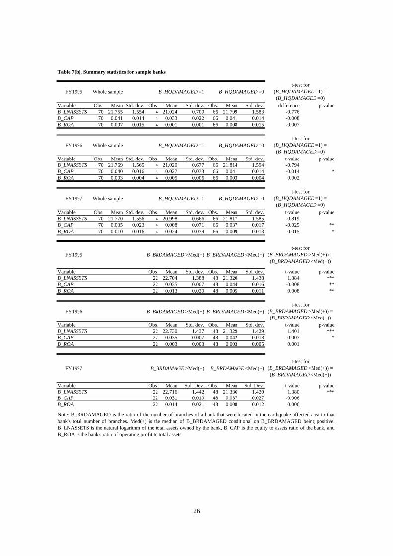
Table 7(b) shows the summary statistics of bank characteristics over the three years, taking each
bank as one observation. In the upper three panels, the first column shows the statistics for all the main
banks of our sample firms, and the second and third columns respectively show the statistics for the banks
headquartered inside or outside the affected area (B_HQDAMAGED=1 or 0), in each of the three years. In
the two columns in the lower three panels, we classify banks according to the extent of branch damage

13
(i.e. whether B_BRDAMAGED is greater than the median value).16 We find that the differences in means
of the bank characteristic variables between banks above and below the median in terms of
B_BRDAMAGED are mostly statistically significant. However, this does not necessarily mean that the
financial conditions of damaged banks were worse than those of their undamaged peers. Although B_CAP
is higher for banks with a smaller B_BRDAMAGED in all three years, B_ROA in FY 1995 is higher for
banks with a greater B_BRDAMAGED than those with a smaller B_BRDAMAGED. Since the bank
characteristic variables are potentially correlated with banks’ capability to provide loans, we need to
control properly for such characteristics in our empirical analysis. Finally, we check the correlation
coefficients for firm and bank characteristics (not reported) and find that no significant correlation is
observed between any pair of explanatory variables, implying that we do not need worry about
multicollinearity.
6. Regression Results
6.1 Baseline results
The results for the baseline estimation are shown in Table 8. For each year, we report the results for
two specifications: one using (1) B_HQDAMAGED and the other using (2) B_BRDAMAGED as the bank
damage variable (referred to as B_DAMAGED). We find that F_SALESGROWTH, the proxy for Q, takes
a positive coefficient in all years for both specifications, and is statistically significant in FY1995 and
FY1997. F_DAMAGED has a positive and significant coefficient in all three years for specification (1),
and in FY1997 for specification (2), implying that the capital investment ratio of affected firms increased
after the earthquake as they recovered from the damage. For example, the results for specification (1)
show that when associated with an undamaged main bank, the investment ratios of damaged firms were
higher by 2.4, 2.3 and 2.8 percentage points respectively in FY1995, FY1996 and FY1997 than those of
undamaged firms.
Turning to our variables of primary interest, we find that B_DAMAGED has a negative and
significant coefficient in either FY1995 (for specification (1)) or FY1996 (for specification (2)), implying
that the investment ratio of firms that were not hit by the earthquake was adversely affected if their main
bank was hit. Since damage to banks is an exogenous financial shock for firms located outside the
earthquake-hit area, this result strongly suggests that exogenous shocks to bank lending capacity
generally affect client firm investment. The impact of bank damage on undamaged firms is economically
significant as well. For specification (1), where bank damage is defined as headquarters damage, the
16 The median is computed using only those banks with a positive value for B_BRDAMAGE. Banks with a zero value for B_BRDAMAGE are classified as being below the median.

14
investment ratio of undamaged firms associated with damaged main banks is smaller by 8.1 percentage
points than that of undamaged firms associated with undamaged main banks. This impact is economically
significant, given that the average investment ratio for undamaged firms in FY1995 was 13.1%. For
specification (2), where bank damage is represented by branch damage, the investment ratio of
undamaged firms associated with damaged main banks whose value of B_BRDAMAGED equals to its
sample mean of the undamaged firms (i.e., 7 percentage points) in FY1996 had investment ratios that
were lower by 1.0 percentage points compared with firms with undamaged main banks. The quantitative
impact is again economically significant.
An interesting finding is that the timing of the impact of bank damage on firm investment differs
between the two specifications. While the negative and significant impact of B_HQDAMAGED on client
firms’ investment manifested itself immediately after the earthquake, i.e., in FY1995, the significant
impact of B_BRDAMAGED did so only one year later in FY1996. This difference might stem from what
these variables represent. B_HQDAMAGED captures the impairment to a bank’s back-office operations at
the headquarters, such as making decisions on whether to accept or reject applications for large loans,
while B_BRDAMAGED reflects the damage to a bank’s ability to process applications for small loans,
and/or loan portfolio losses caused by the deterioration in local borrowers’ financial conditions due to the
earthquake. Note that the effects of bank damage, either to headquarters or to branch networks, are
short-lived. The coefficient of B_HQDAMAGED turns positive and significant in FY 1997, possibly
reflecting a recovery from the low investment caused by bank damage in FY1995, while
B_BRDAMAGED is not significant in FY 1997.
Turning to the interaction term of bank damage and firm damage, the sum of B_DAMAGED and the
interaction term of F_DAMAGED and B_DAMAGED is positive and marginally significant at the 10%
level in FY1995 (for specification (1)), suggesting that bank damage positively affected damaged firms’
investment. This might imply that damaged banks shifted their loan portfolios from undamaged to
damaged firms to assist the damaged firms’ recovery, but the result is not strongly significant and is
observed only in FY1995.
All the variables representing firms’ financial constraints have coefficients with the expected signs,
although the level of statistical significance varies across variables and years. F_ROA and F_CASH have
significantly positive coefficients in all years in both specifications, while F_ LNASSET has significantly
positive coefficients in FY1996 and FY1997, and F_LEV has a significantly negative coefficient in
FY1995.
Finally, the coefficients on the variables for banks’ lending capacity have inconsistent signs over
time, and none of the coefficients are significant. These results are consistent with the view that banks’
15
balance sheet variables at the time might not have reflected their true financial conditions.
6.2 Differences by bank size
In the baseline estimation, we did not distinguish between banks of different sizes. Compared
with larger regional banks, Shinkin banks (shinyo kinko in Japanese) and credit cooperatives (shinyo
kumiai in Japanese), both of which are small credit unions, tend to operate in more concentrated
geographical areas.17 Consequently, it may be more difficult for these banks to diversify their loan
portfolios, so they might be more vulnerable than others if struck by an earthquake. To the extent that this
is the case, firms associated with a damaged Shinkin bank or credit cooperative may have been affected
more severely.
To take this possibility into account, we now introduce an interaction term interacting
B_HQDAMAGED or B_BRDAMAGED with a small bank dummy, SMALL, which takes a value of one if
a firm’s main bank is either a Shinkin bank or a credit cooperative. The interaction term is expected to
have a negative sign. Note that in this specification, we implicitly assume that damage to regional banks,
which are relatively large, has no significant impact on their client firms’ investment, because these banks
are likely to have more diversified loan portfolios than Shinkin banks and credit cooperatives.
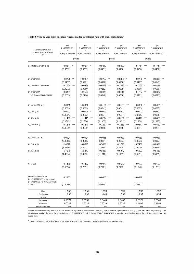
Table 9 shows the results. In specification (1), where B_HQDAMAGE is interacted with SMALL,
the coefficient on the interaction term is negative and statistically significant both in FY1995 (as in the
baseline case) and in FY1996 (unlike in the baseline case). In FY1995, the absolute value of the
coefficient is larger than that of B_HQDAMAGE in the baseline result. That is, the investment ratio of
undamaged firms associated with damaged Shinkin banks or credit cooperatives was lower by 10.0
percentage points than that of undamaged firms associated with undamaged (or damaged regional) main
banks. These results are consistent with our prediction that firms associated with a damaged small bank
are more severely affected than those associated with a damaged large bank. The interaction term of
B_HQDAMAGED and SMALL has a positive and significant coefficient in FY1997, but its absolute value
is smaller than the coefficient of B_HQDAMAGED in the baseline result, suggesting that the recovery
from the period of depressed investment was weaker for firms associated with small banks. In
specification (2) where we interact B_BRDAMAGED with SMALL, the coefficient of the interaction term
is significant and negative for FY1996 (as in the baseline result).
17 Regional banks are generally smaller than city banks but larger than Shinkin banks and credit cooperatives in Japan. A more detailed description of the various types of banks in Japan, including regional banks and Shinkin banks, can be found in Uchida and Udell (2010).
16
Note that the results for all the other explanatory variables are similar to those in the baseline
estimation for both specifications, except that the sum of the coefficients on B_DAMAGED and on the
interaction term of F_DAMAGED and B_HQDAMAGED (interacted with SMALL) is not statistically
significant. The latter result suggests that the portfolio shift effect observed in the baseline estimation is
not found when we focus on small banks only.
6.3 Controlling for firm fixed effects
Thus far we have conducted cross-sectional regressions, based on the assumption that before the
earthquake, firms’ investment was not significantly different between damaged and undamaged firms.
This assumption is plausible, given that the earthquake was an exogenous shock to firms. However, for
the sake of robustness, we attempt to ascertain whether controlling for the difference in the
pre-earthquake investment ratio among firms changes our results. Here we explicitly control for the
unobservable firm-level fixed effect by differencing the investment ratio as follows:
)2(.1997,1996,1995___*_
___
16
1,51,4
13211094
94
=++
++
+++=−
−
−−
−−
tforCAPACITYBSCONSTRAINTFDAMAGEDBDAMAGEDF
DAMAGEDBDAMAGEDFHSALESGROWTFKI
KI
itit
titii
itiiti
i
it
it
εβ
ββ
ββββ
The dependent variable now is the difference in investment ratio between the post-earthquake
period (in FY1995, FY1996, and FY1997) and the pre-earthquake period (FY1994). Because the BSBSA
database contains firm characteristic data only from FY1994, the information on capital stock as of
FY1993 ( 93iK ) is not available. We therefore include a rather unconventional variable: the ratio of
investment to the contemporaneous end-of-period capital stock ( itit KI / ) rather than the ratio of
investment to the previous end-of-period capital stock ( 1/ −itit KI ). Because the information on firm
characteristics as of FY1993 ( 93_ iSCONSTRAINTF ) is also unavailable, we do not difference the
explanatory variables.18
The results are shown in Table 10. F_SALESGROWTH has a positive coefficient in all years and is
significant in FY1997 for specification (2). More importantly, B_HQDAMAGED has a negative and
significant coefficient in FY1995 (first column), while B_BRDAMAGED has a negative and significant
18 We obtained the information on sales in FY1993 from the TDB database in order to construct the variable 94,_ iHSALESGROWTF .
17
coefficient in FY1996 (fourth column), both of which are consistent with our baseline results. On the
other hand, when we test whether the sum of the coefficients on B_DAMAGED and on the interaction
term of F_DAMAGED and B_HQDAMAGED is statistically different from zero, we find that the sum is
not significant in any year, suggesting that the portfolio shift effect observed in the baseline estimation is
not robust to an alternative estimation strategy. As for the control variables, F_ROA and F_CASH are
positive and significant in all years for both specifications, and B_ROA has a positive and significant
coefficient in FY1997. Overall, controlling for firm-level fixed effects yields reasonable results and does
not substantially change the results concerning the effects of bank damage on the investment of
undamaged firms.
7. Conclusion
In this paper we investigated whether the lending capacity of banks affects firm investment. To
overcome the difficulties in identifying truly exogenous shocks to the lending capacity of banks, we
utilized the natural experiment provided by the Kobe earthquake. Using a unique firm-level dataset that
allows us to identify firms and banks in the affected area, and combining this dataset with information on
bank-firm relationships and financial statements, we examined the impact that a transactional relationship
with a bank in the affected area had on the post-earthquake investment of client firms that were not
themselves directly affected by the earthquake.
We found that the investment ratio of firms located outside the earthquake-affected area but
having a main bank inside the area was smaller than that of firms whose main bank was outside the
affected area. This result implies that the weakened lending capacity of damaged banks exacerbated
borrowing constraints on the investment of their client firms. In addition, we found that the negative
impact is robust to whether bank damage is measured as damage to the bank’s headquarters or damage to
its branch network. However, while the impact of headquarters damage emerged immediately after the
earthquake, the impact of branch damage appeared only with a one-year lag. This difference in the timing
of the impacts suggests that there were two different channels through which damage to banks affected
client firms: through the impairment of banks’ managerial capacity to originate loans, and through the
impairment of their risk-taking capacity. It is also noteworthy that bank damage, either to headquarters or
branch networks, did not last for a long time; by three years after the earthquake, the effect had dissipated.

18
Reference
Abel, A. B., Eberly, J. C., 2011. How Q and Cash Flow Affect Investment Without Frictions: An Analytic
Explanation. Review of Economic Studies 78, pp. 1179-1200.
Acharya, V. V., Almeida, H., and Campello, M., 2007. Is Cash Negative Debt? A Hedging Perspective on
Corporate Financial Policies. Journal of Financial Intermediation 16, pp. 515-554.
Ashcraft, A. B., 2005. Are Banks Really Special? New Evidence from the FDIC-Induced Failure of
Healthy Banks. American Economic Review 95 (5), pp. 1712-1730.
Bae, K-H., Kang, J.-K., Lim, C.-W., 2002. The Value of Durable Bank Relationships: Evidence from
Korean Banking Shocks. Journal of Financial Economics 64, pp. 181-214.
Bayer, C., 2006. Investment Dynamics with Fixed Capital Adjustment Cost and Capital Market
Imperfections. Journal of Monetary Economics 53, pp.1909-1947.
Berg, G., Schrader, J., 2012. Access to Credit, Natural Disasters, and Relationship Lending. Journal of
Financial Intermediation 21, pp. 549-568.
Bernanke, B. S., 1983. Nonmonetary Effects of the Financial Crisis in the Propagation of the Great
Depression. American Economic Review 73 (3), pp. 257-276.
Bernanke, B. S., Lown, C. S., 1991. The Credit Crunch. Brookings Papers on Economic Activity, 1991,
(2), pp. 205-48.
Brewer III, E., Ganay, H., Hunter, C. W., Kaufman, G. G., 2003a. The Value of Banking Relationships
During a Financial Crisis: Evidence from Failures of Japanese Banks. Journal of the Japanese and
International Economies 17, pp. 233-262.
Brewer, E. III, Genay, H., Hunter, W. C., Kaufman, G. G., 2003b. Does the Japanese Stock Market Price
Bank-Risk? Evidence from Financial Firm Failures. Journal of Money, Credit, and Banking 35 (4), pp.
507-543.
Buera, F., Kaboski, J. P., Shin, Y. 2011. Finance and Development: A Tale of Two Sectors. American
Economic Review 101(5), pp.1964-2002.
Caballero, R. J., Hoshi, T., Kashyap, A. K., 2008. Zombie Lending and Depressed Restructuring in Japan.
American Economic Review 98 (5), pp. 1943-1977.
Calomiris, C. W., Mason, J. R., 2003. Consequences of Bank Distress During the Great Depression.
American Economic Review 93 (3), pp. 937-947.
Cetorelli, N., Goldberg, L. S., 2012. Follow the Money: Quantifying Domestic Effects of Foreign Bank
Shocks in the Great Recession. American Economic Review, Vol. 102, No. 3, pp. 313-218.
Chava, S., Purnanandam, A., 2011. The Effect of Banking Crisis on Bank-Dependent Borrowers. Journal
of Financial Economics 99, pp. 116-135.
Crespo-Cuaresma, J., Hlouskova, J., Obersteiner, M., 2008. Natural Disasters as Creative Destruction?
Evidence from Developing Countries. Economic Inquiry 46 (2), pp. 214-226.

19
De Mel, S., McKenzie, D., Woodruff, C., 2011. Enterprise Recovery Following Natural Disasters.
Economic Journal 122, pp. 64-91.
Fukuda, S., Koibuchi, S., 2007. The Impacts of “Shock Therapy” on Large and Small Clients:
Experiences from Two Large Bank Failures in Japan. Pacific-Basin Finance Journal 15, pp, 434-451.
Gibson, M. S., 1995. Can Bank Health Affect Investment? Evidence from Japan. Journal of Business, 68
(3), pp. 281-308.
Gibson, M. S., 1997. More Evidence on the Link Between Bank Health and Investment in Japan. Journal
of the Japanese and International Economies 11 (3), pp. 296-310.
Gomes, J. F., 2001. Financing Investment. American Economic Review 91, pp. 1263-1285.
Hennessy, C. A., Levy, A., Whited, T., 2007. Testing Q Theory with Financing Frictions. Journal of
Financial Economics 83, pp. 691-717.
Hori, M., 2005. Does Bank Liquidation Affect Client Firm Performance? Evidence from a Bank Failure
in Japan. Economics Letters 88, pp. 415-420.
Hsieh, C. Klenow, P. J., 2009. Misallocation and Manufacturing TFP in China and India. Quarterly
Journal of Economics 124(2), pp.1403–1448.
Ito, T., Sasaki, Y. N., 2002. Impacts of the Basel Capital Standards on Japanese Banks’ Behavior. Journal
of the Japanese International Economies 16 (3), pp.372-397.
Kahn, M. E., 2005. The Death Toll from Natural Disasters: The Role of Income, Geography, and
Institutions. Review of Economics and Statistics 87(2), 272-284.
Khwaja, A. I., Mian, A, 2008. Tracing the Impact of Bank Liquidity Shocks: Evidence from an Emerging
Market. American Economic Review 98 (4), pp. 1413-1412.
Leiter, A. M., Oberhofer, H., Raschky, P. A., 2009. Creative Disasters? Flooding Effects on Capital,
Labor and Productivity Within European Firms. Environmental and Resource Economics 43, pp.
333-350.
Minamihashi, N., 2011. Credit Crunch Caused by Bank Failures and Self-Selection Behavior in Lending
Markets. Journal of Money, Credit and Banking 43 (1), pp. 133-161.
Nagahata, T., Sekine, T., 2005. Firm Investment, Monetary Transmission and Balance-Sheet Problems in
Japan: An Investigation Using Micro Data. Japan and the World Economy 17(3), 345-69.
Okuyama, Y., 2003. Economics of Natural Disasters: A Critical Review. Research Paper 2003-12,
Regional Research Institute, West Virginia University.
Paravisini, D., V. Rappoport, P. Schnabl, and D. Wolfenzon., 2011, Dissecting the Effect of Credit
Supply on Trade: Evidence from Matched Credit-Export Data. NBER Working Paper 16975.
Peek, J., Rosengren, E. S., 2000. Collateral Damage: Effects of the Japanese Bank Crisis on Real Activity
in the United States. American Economic Review 90 (1), pp. 30-45.
Peek, J., Rosengren, E. S., 2005. Unnatural Selection: Perverse Incentives and the Misallocation of Credit
in Japan. American Economic Review 95 (4), pp. 1144-1166.
20
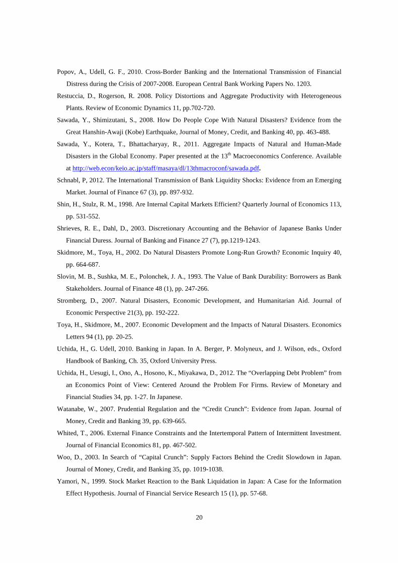
Popov, A., Udell, G. F., 2010. Cross-Border Banking and the International Transmission of Financial
Distress during the Crisis of 2007-2008. European Central Bank Working Papers No. 1203.
Restuccia, D., Rogerson, R. 2008. Policy Distortions and Aggregate Productivity with Heterogeneous
Plants. Review of Economic Dynamics 11, pp.702-720.
Sawada, Y., Shimizutani, S., 2008. How Do People Cope With Natural Disasters? Evidence from the
Great Hanshin-Awaji (Kobe) Earthquake, Journal of Money, Credit, and Banking 40, pp. 463-488.
Sawada, Y., Kotera, T., Bhattacharyay, R., 2011. Aggregate Impacts of Natural and Human-Made
Disasters in the Global Economy. Paper presented at the 13th Macroeconomics Conference. Available
at http://web.econ/keio.ac.jp/staff/masaya/dl/13thmacroconf/sawada.pdf.
Schnabl, P, 2012. The International Transmission of Bank Liquidity Shocks: Evidence from an Emerging
Market. Journal of Finance 67 (3), pp. 897-932.
Shin, H., Stulz, R. M., 1998. Are Internal Capital Markets Efficient? Quarterly Journal of Economics 113,
pp. 531-552.
Shrieves, R. E., Dahl, D., 2003. Discretionary Accounting and the Behavior of Japanese Banks Under
Financial Duress. Journal of Banking and Finance 27 (7), pp.1219-1243.
Skidmore, M., Toya, H., 2002. Do Natural Disasters Promote Long-Run Growth? Economic Inquiry 40,
pp. 664-687.
Slovin, M. B., Sushka, M. E., Polonchek, J. A., 1993. The Value of Bank Durability: Borrowers as Bank
Stakeholders. Journal of Finance 48 (1), pp. 247-266.
Stromberg, D., 2007. Natural Disasters, Economic Development, and Humanitarian Aid. Journal of
Economic Perspective 21(3), pp. 192-222.
Toya, H., Skidmore, M., 2007. Economic Development and the Impacts of Natural Disasters. Economics
Letters 94 (1), pp. 20-25.
Uchida, H., G. Udell, 2010. Banking in Japan. In A. Berger, P. Molyneux, and J. Wilson, eds., Oxford
Handbook of Banking, Ch. 35, Oxford University Press.
Uchida, H., Uesugi, I., Ono, A., Hosono, K., Miyakawa, D., 2012. The “Overlapping Debt Problem” from
an Economics Point of View: Centered Around the Problem For Firms. Review of Monetary and
Financial Studies 34, pp. 1-27. In Japanese.
Watanabe, W., 2007. Prudential Regulation and the “Credit Crunch”: Evidence from Japan. Journal of
Money, Credit and Banking 39, pp. 639-665.
Whited, T., 2006. External Finance Constraints and the Intertemporal Pattern of Intermittent Investment.
Journal of Financial Economics 81, pp. 467-502.
Woo, D., 2003. In Search of “Capital Crunch”: Supply Factors Behind the Credit Slowdown in Japan.
Journal of Money, Credit, and Banking 35, pp. 1019-1038.
Yamori, N., 1999. Stock Market Reaction to the Bank Liquidation in Japan: A Case for the Information
Effect Hypothesis. Journal of Financial Service Research 15 (1), pp. 57-68.

21
Yamori, N., Murakami, A., 1999. Does Bank Relationship Have an Economic Value? The Effect of Main
Bank Failure on Client Firms. Economics Letters 65, pp. 115-120.

22
Tables
Table 1. Estimated damage caused by the Kobe earthquake
No. ofdeaths
No. ofhousing
unitscompletelydestroyed
No. ofhousing
units partlydestroyed
Death rate
Rate ofhousing
unitscompletelydestroyed
Rate ofhousing
units partlydestroyed
Rate ofhousing
unitscompletely
or partlydestroyed
Regions in designated disaster area 6,405 104,455 140,681 0.17% 16.50% 22.23% 38.73%Kobe City Higashinada-ku 1,470 12,832 5,085 0.77% 50.50% 20.01% 70.51%
Nada-ku 931 11,795 5,325 0.72% 54.13% 24.44% 78.57%Hyogo-ku 553 8,148 7,317 0.45% 35.55% 31.92% 67.47%Nagata-ku 917 14,662 7,770 0.67% 60.21% 31.91% 92.12%Suma-ku 401 7,466 5,344 0.21% 27.68% 19.81% 47.50%Tarumi-ku 25 1,087 8,575 0.01% 2.78% 21.95% 24.73%Kita-ku 13 251 3,029 0.01% 0.63% 7.67% 8.31%Chuo-ku 243 5,156 5,533 0.21% 33.39% 35.84% 69.23%Nishi-ku 9 403 3,147 0.01% 1.19% 9.28% 10.46%
Amagasaki City 49 5,688 36,002 0.01% 7.60% 48.07% 55.67%Nishinomiya City 1,126 20,667 14,597 0.26% 31.30% 22.11% 53.41%Ashiya City 443 3,915 3,571 0.51% 31.67% 28.89% 60.57%Itami City 22 1,395 7,499 0.01% 4.39% 23.57% 27.96%Takarazuka City 117 3,559 9,313 0.06% 9.12% 23.86% 32.98%Kawanishi City 4 554 2,728 0.00% 1.56% 7.70% 9.26%Akashi City 11 2,941 6,673 0.00% 5.51% 12.51% 18.02%Sumoto City 4 203 932 0.01% 1.71% 7.83% 9.54%Awaji City 58 3,076 3,976 0.11% NA NA NAToyonaka City 9 657 4,265 0.00% 1.12% 7.27% 8.39%Regions outside designated area 22 445 3,427 0.00% 0.04% 0.30% 0.33%
Note: "Regions outside designated area" refers to regions that are in Hyogo and Osaka prefectures but were not included in theAct Concerning Special Financial Support to Deal with a Designated Disaster of Extreme Severity. All rates for these regionsare the averages of all cities and towns in these regions. The Act Concerning Special Financial Support to Deal with aDesignated Disaster of Extreme Severity covered nine cities and five towns. One of the towns has since been merged intoSumoto City, while the other four have been merged together to form Awaji City. The table here shows the casualties andhousing damage for the merged entities. The number of deaths and the numbers of destroyed housing units were compiled bythe Fire and Disaster Management Agency and are as of May 19, 2006. To calculate the rates, we used data from the 1990Population Census and the 1993 Housing and Land Survey. The figures on the losses of housing units are taken from<http://web.pref.hyogo.jp/pa20/pa20_000000006.html>. The table covers all cities and towns in Hyogo Prefecture as well assome in Osaka Prefecture (for a total of nine cities and five towns in the two prefectures combined), which were included in theAct Concerning Special Financial Support to Deal with a Designated Disaster of Extreme Severity.To calculate the ratio of thenumber of casualties to the total population and the ratios of the numbers of completely and partly destroyed housing units tothe total number of housing units, we used data from the 1990 Population Census (Ministry of Internal Affairs andCommunications, Government of Japan) and the 1993 Housing and Land Survey (Ministry of Construction).
23
Table 2. Bank branch operations after the earthquake
Operated Did Not OperateCity banks 11 227 125 102Long-term banks 2 2 0 2Trust banks 6 17 10 7Regional banks 13 122 72 50Regional banks 2 12 254 106 148Shinkin banks 15 422 325 97Credit Cooperatives 15 111 77 34Total 74 1155 715 440
Type of banks No. of banks No. of branches As of Jan 18, 1995
Note. The sample is limited to those financial institutions whose branches were located inHyogo prefecture. "Regional banks 2" refers to member banks of the Second Association ofRegional Banks. Shinkin banks (shinyo kinko in Japanese) and credit cooperatives (shinyokumiai in Japanese) are small credit unions. The data source is the Bank of Japan.
Table 3. Banks headquartered in the earhtquake-affected area
PrefectureLoans outstanding(100 million yen)
No. of branches
Osaka Suito Shinkin Shinkin bank 1,720 19
Howa Shinso Credit cooperative 377 8
Hyogo Hyogo Bank Regional bank 2 27,443 147
Hanshin Bank Regional bank 2 8,772 80
6 Shinkins (total) 19,752 192
8 credit unions (total) 4,381 66
Name and type of financial institution
Note: Regional bank 2 refers to a member bank of the Second Association of Regional Banks. Shinkin banks(shinyo kinko in Japanese) and credit cooperatives (shinyo kumiai in Japanese) are small credit unions.Theearthquake-affected area comprises 8 cities and 5 towns (among them Kobe City itself) in Hyogo prefectureand 1 city (Toyonaka City) in Osaka prefecture. The data sources are Nikkei NEEDS Financial Quest,Financial Statements of Shinkin Banks in Japan, and Financial Statements of Credit Cooperatives in Japan.

24
Table 4. Share of firms dropped from the sample
No. of firms observed in FY1994 No. of firms dropped out of the sampleFY1994 FY1995 FY1996 FY1997
Full sample 3,212 430 612 895(Percentage) 100.0% 13.4% 19.1% 27.9%
F_DAMAGED = 0 2,621 364 513 727(Percentage) 100.0% 13.9% 19.6% 27.7%F_DAMAGED = 1 591 66 99 168(Percentage) 100.0% 11.2% 16.8% 28.4%
B_DAMAGED = 0 3,157 421 597 876(Percentage) 100.0% 13.3% 18.9% 27.7%B_DAMAGED = 1 55 9 15 19(Percentage) 100.0% 16.4% 27.3% 34.5% Table 5. Industry composition
No. of firms Share No. of firms ShareAgriculture, forestry and fisheries 0 0.0 0 0.0Mining 0 0.0 0 0.0Construction 8 2.3 23 1.4Manufacturing 220 62.7 910 56.7Wholesale 80 22.8 552 34.4Retail and restaurants 35 10.0 102 6.4Services 8 2.3 17 1.1Other 0 0.0 0 0.0Total 351 100.0 1,604 100.0Note. The observation period is FY1995.
F_DAMAGED = 1 F_DAMAGED = 0
Table 6. Fraction of firms that switched their main banks
No. of firms in FY1994 No. of firms that switched their main banksFY1994 FY1995 FY1996 FY1997
Full sample 2,094 57 81 124(Percentage) 100.0% 2.7% 3.9% 5.9%
F_DAMAGED = 0 1,703 41 65 94(Percentage) 100.0% 2.4% 3.8% 5.5%F_DAMAGED = 1 391 16 16 30(Percentage) 100.0% 4.1% 4.1% 7.7%

25
Table 7(a). Summary statistics for sample firms
FY1995
Whole sample F_DAMAGED =1 F_DAMAGED =0
Variable Obs. Mean Std. dev. Obs. Mean Std. dev. Obs. Mean Std. dev. difference p-valueF_INVESTMENTRATIO 1,955 0.136 0.231 351 0.158 0.264 1,604 0.131 0.223 0.0268 **F_SALESGROWTH 1,955 0.003 0.106 351 -0.011 0.126 1,604 0.007 0.101F_LNASSETS 1,955 8.659 1.269 351 8.516 1.306 1,604 8.690 1.259F_LEV 1,955 6.800 12.423 351 5.415 8.988 1,604 7.103 13.037F_ROA 1,955 0.028 0.043 351 0.023 0.050 1,604 0.029 0.041F_CASH 1,955 0.635 0.167 351 0.625 0.165 1,604 0.637 0.167F_DAMAGED 1,955 0.180 0.384 351 1.000 0.000 1,604 0.000 0.000B_LNASSETS 1,955 24.151 1.086 351 24.209 1.086 1,604 24.139 1.086 0.0700B_CAP 1,955 0.036 0.004 351 0.036 0.004 1,604 0.036 0.004 -0.0002B_ROA 1,955 0.003 0.004 351 0.003 0.003 1,604 0.004 0.004 -0.0002B_HQDAMAGED 1,955 0.008 0.087 351 0.031 0.174 1,604 0.002 0.050 0.0288 ***B_BRDAMAGED 1,955 0.077 0.089 351 0.113 0.138 1,604 0.070 0.072 0.0434 ***
FY1996
Whole sample F_DAMAGED =1 F_DAMAGED =0
Variable Obs. Mean Std. dev. Obs. Mean Std. dev. Obs. Mean Std. dev. difference p-valueF_INVESTMENTRATIO 1,990 0.140 0.228 362 0.156 0.229 1,628 0.136 0.228 0.0202F_SALESGROWTH 1,990 0.020 0.111 362 0.022 0.141 1,628 0.020 0.103F_LNASSETS 1,990 8.679 1.266 362 8.532 1.285 1,628 8.712 1.260F_LEV 1,990 6.761 12.626 362 6.151 11.375 1,628 6.897 12.887F_ROA 1,990 0.029 0.041 362 0.026 0.045 1,628 0.029 0.040F_CASH 1,990 0.635 0.168 362 0.623 0.173 1,628 0.638 0.167F_DAMAGED 1,990 0.182 0.386 362 1.000 0.000 1,628 0.000 0.000B_LNASSETS 1,990 24.175 1.100 362 24.216 1.097 1,628 24.166 1.100 0.0499B_CAP 1,990 0.031 0.005 362 0.031 0.006 1,628 0.032 0.005 -0.0007 **B_ROA 1,990 0.007 0.008 362 0.009 0.010 1,628 0.007 0.008 0.0018 ***
FY1997
Whole sample F_DAMAGED =1 F_DAMAGED =0
Variable Obs. Std. dev. Std. Dev. Obs. Mean Std. dev. Obs. Mean Std. dev. difference p-valueF_INVESTMENTRATIO 1,997 0.135 0.205 366 0.151 0.219 1,631 0.131 0.202 0.0200 *F_SALESGROWTH 1,997 0.032 0.098 366 0.024 0.123 1,631 0.033 0.091F_LNASSETS 1,997 8.702 1.278 366 8.540 1.289 1,631 8.739 1.273F_LEV 1,997 6.593 12.781 366 5.188 9.274 1,631 6.908 13.425F_ROA 1,997 0.033 0.039 366 0.030 0.041 1,631 0.033 0.039F_CASH 1,997 0.635 0.170 366 0.614 0.174 1,631 0.639 0.169F_DAMAGED 1,997 0.183 0.387 366 1.000 0.000 1,631 0.000 0.000B_LNASSETS 1,997 24.223 1.118 366 24.258 1.139 1,631 24.216 1.113 0.0421B_CAP 1,997 0.032 0.005 366 0.031 0.005 1,631 0.032 0.005 -0.0004B_ROA 1,997 0.003 0.005 366 0.003 0.003 1,631 0.003 0.005 0.0000
t-test for(F_DAMAGED =1) =(F_DAMAGED =0)
t-test for(F_DAMAGED =1) =(F_DAMAGED =0)
t-test for(F_DAMAGED =1) =(F_DAMAGED =0)
Note: F_INVESTMENTRATIO is the ratio of firms’ capital investment to one-period lagged fixed assets, F_SALESGROWTH isthe growth rate of firms’ sales, F_LNASSETS is the natural logarithm of firms’ total assets, F_LEV is the ratio of firms’ liabilitiesto equity, F_ROA is the ratio of firms’ current profit to total assets, F_CASH is the ratio of firms’ liquid assets to total assets,F_DAMAGED is a dummy variable taking a value of one if the firm is located in one of the cities or towns identified as affectedby the earthquake in the Act on Special Financial Support to Deal with a Designated Disaster of Extreme Severity, B_LNASSETS isthe natural logarithm of the total assets owned by a firm's main bank, B_CAP is the equity to assets ratio of a firm's main bank,B_ROA is the ratio of operating profit to total assets of a firm's main bank, B_HQDAMAGED is a dummy variable taking a valueof one if the headquarters of a firm’s main bank is located in the earthquake-affected area, and B_BRDAMAGED is the ratio of thenumber of branches of a firm’s main bank located in the earthquake-affected area to the total number of branches of that bank.
26
Table 7(b). Summary statistics for sample banks
FY1995 Whole sample B_HQDAMAGED =1 B_HQDAMAGED =0
Variable Obs. Mean Std. dev. Obs. Mean Std. dev. Obs. Mean Std. dev. difference p-valueB_LNASSETS 70 21.755 1.554 4 21.024 0.700 66 21.799 1.583 -0.776B_CAP 70 0.041 0.014 4 0.033 0.022 66 0.041 0.014 -0.008B_ROA 70 0.007 0.015 4 0.001 0.001 66 0.008 0.015 -0.007
FY1996 Whole sample B_HQDAMAGED =1 B_HQDAMAGED =0
Variable Obs. Mean Std. dev. Obs. Mean Std. dev. Obs. Mean Std. dev. t-value p-valueB_LNASSETS 70 21.769 1.565 4 21.020 0.677 66 21.814 1.594 -0.794B_CAP 70 0.040 0.016 4 0.027 0.033 66 0.041 0.014 -0.014 *B_ROA 70 0.003 0.004 4 0.005 0.006 66 0.003 0.004 0.002
FY1997 Whole sample B_HQDAMAGED =1 B_HQDAMAGED =0
Variable Obs. Mean Std. dev. Obs. Mean Std. dev. Obs. Mean Std. dev. t-value p-valueB_LNASSETS 70 21.770 1.556 4 20.998 0.666 66 21.817 1.585 -0.819B_CAP 70 0.035 0.023 4 0.008 0.071 66 0.037 0.017 -0.029 **B_ROA 70 0.010 0.016 4 0.024 0.039 66 0.009 0.013 0.015 *
FY1995 B_BRDAMAGED >Med(+) B_BRDAMAGED <Med(+)
Variable Obs. Mean Std. dev. Obs. Mean Std. dev. t-value p-valueB_LNASSETS 22 22.704 1.388 48 21.320 1.438 1.384 ***B_CAP 22 0.035 0.007 48 0.044 0.016 -0.008 **B_ROA 22 0.013 0.020 48 0.005 0.011 0.008 **
FY1996 B_BRDAMAGED >Med(+) B_BRDAMAGED <Med(+)
Variable Obs. Mean Std. dev. Obs. Mean Std. dev. t-value p-valueB_LNASSETS 22 22.730 1.437 48 21.329 1.429 1.401 ***B_CAP 22 0.035 0.007 48 0.042 0.018 -0.007 *B_ROA 22 0.003 0.003 48 0.003 0.005 0.001
FY1997 B_BRDAMAGE >Med(+) B_BRDAMAGE <Med(+)
Variable Obs. Mean Std. Dev. Obs. Mean Std. Dev. t-value p-valueB_LNASSETS 22 22.716 1.442 48 21.336 1.420 1.380 ***B_CAP 22 0.031 0.010 48 0.037 0.027 -0.006B_ROA 22 0.014 0.021 48 0.008 0.012 0.006
t-test for(B_BRDAMAGED >Med(+)) =(B_BRDAMAGED <Med(+))
Note: B_BRDAMAGED is the ratio of the number of branches of a bank that were located in the earthquake-affected area to thatbank's total number of branches. Med(+) is the median of B_BRDAMAGED conditional on B_BRDAMAGED being positive.B_LNASSETS is the natural logarithm of the total assets owned by the bank, B_CAP is the equity to assets ratio of the bank, andB_ROA is the bank's ratio of operating profit to total assets.
t-test for(B_HQDAMAGED =1) =(B_HQDAMAGED =0)
t-test for(B_HQDAMAGED =1) =(B_HQDAMAGED =0)
t-test for(B_HQDAMAGED =1) =(B_HQDAMAGED =0)
t-test for(B_BRDAMAGED >Med(+)) =(B_BRDAMAGED <Med(+))
t-test for(B_BRDAMAGED >Med(+)) =(B_BRDAMAGED <Med(+))

27
F_SALESGROWTH (t-1) 0.0960 * 0.1006 * 0.0452 0.0437 0.1712 *** 0.1741 ***
(0.0529) (0.0528) (0.0479) (0.0480) (0.0490) (0.0490)
F_DAMAGED 0.0244 * -0.0042 0.0233 * 0.0182 0.0281 ** 0.0327 **
(0.0134) (0.0205) (0.0128) (0.0171) (0.0127) (0.0144) B_DAMAGED † -0.0815 *** -0.0396 -0.0290 -0.1273 ** 0.1713 *** 0.0061
(0.0230) (0.0558) (0.0297) (0.0593) (0.0666) (0.0611) F_DAMAGED 0.3578 ** 0.3473 * 0.0721 0.1037 -0.2114 *** -0.0578 ×B_DAMAGED † (0.1678) (0.1893) (0.0706) (0.1001) (0.0778) (0.0866)
F_LNASSETS (t-1) 0.0056 0.0056 0.0167 *** 0.0165 *** 0.0067 * 0.0066 *
(0.0039) (0.0039) (0.0041) (0.0041) (0.0035) (0.0035) F_LEV (t-1) -0.0004 * -0.0005 * 0.0000 0.0000 0.0002 0.0002
(0.0002) (0.0002) (0.0004) (0.0004) (0.0006) (0.0006) F_ROA (t-1) 1.1521 *** 1.1452 *** 0.8211 *** 0.8183 *** 0.8451 *** 0.8461 ***
(0.1502) (0.1504) (0.1404) (0.1402) (0.1227) (0.1227) F_CASH (t-1) 0.1228 *** 0.1229 *** 0.1270 *** 0.1250 *** 0.0850 *** 0.0857 ***
(0.0333) (0.0332) (0.0347) (0.0348) (0.0250) (0.0250)
B_LNASSETS (t-1) -0.0005 -0.0002 -0.0032 -0.0052 -0.0009 -0.0016(0.0061) (0.0065) (0.0062) (0.0065) (0.0043) (0.0045)
B_CAP (t-1) -0.9513 -0.5902 0.5575 0.2849 -0.7586 -0.8526(1.2277) (1.2463) (1.2171) (1.2216) (0.9377) (0.9521)
B_ROA (t-1) -1.6745 -1.3800 0.6028 0.6032 -0.6228 -0.6204(1.4629) (1.4998) (1.1214) (1.1178) (0.5936) (0.5971)
Constant 0.1008 0.0825 -0.0309 0.0374 -0.0181 0.0028(0.1928) (0.2017) (0.2088) (0.2196) (0.1237) (0.1303)
0.2764 * 0.0431 -0.0401
(0.1678) (0.0668) (0.0420)
Obs 1,955 1,955 1,990 1,990 1,997 1,997F-value 9.46 8.62 7.05 7.21 8.97 8.47p-value ** ** **
R-squared 0.0811 0.0792 0.0462 0.0472 0.0581 0.0567Root MSE 0.2223 0.2225 0.2239 0.2238 0.1996 0.1998
Industry dummies yes yes yes yes yes yes
Notes: Heteroskedasticity-robust standard errors are reported in parentheses. ***, **, and * indicate significance at the 1, 5, and 10% level, respectively. Thesignificance level of the sum of the coefficients on B_DAMAGED and F_DAMAGED×B_DAMAGED is based on the F-values under the null hypotheses that the sumis zero.
† The B_DAMAGED variable is either B_HQDAMAGED or B_BRDAMAGED as indicated in the column heading.
Table 8. Year-by-year cross-sectional regressions for investment ratio
(1)B_DAMAGED
=B_HQDAMAGED
(2)B_DAMAGED
=B_BRDAMAGED
(1)B_DAMAGED
=B_HQDAMAGED
(2)B_DAMAGED
=B_BRDAMAGED
(1)B_DAMAGED
=B_HQDAMAGED
(2)B_DAMAGED
=B_BRDAMAGED
Sum of coefficients onB_HQDAMAGED andF_DAMAGED *B_HQDAMAGED
Dependent variable:F_INVESTMENTRATIO
(t)
FY1995 FY1996 FY1997
28
F_SALESGROWTH (t-1) 0.0951 * 0.0994 * 0.0432 0.0422 0.1714 *** 0.1745 ***
(0.0532) (0.0532) (0.0481) (0.0480) (0.0490) (0.0490)
F_DAMAGED 0.0276 ** 0.0069 0.0257 ** 0.0306 * 0.0280 ** 0.0316 **
(0.0137) (0.0221) (0.0128) (0.0168) (0.0127) (0.0142) B_DAMAGED †×SMALL -0.1000 *** -0.0429 -0.0579 *** -0.1425 ** 0.1165 * -0.0281
(0.0212) (0.0580) (0.0212) (0.0609) (0.0618) (0.0585) F_DAMAGED 0.3351 0.2627 -0.0025 -0.0116 -0.1764 ** -0.0387 ×B_DAMAGED †×SMALL (0.2055) (0.2126) (0.0348) (0.0860) (0.0711) (0.0872)
F_LNASSETS (t-1) 0.0058 0.0056 0.0166 *** 0.0163 *** 0.0066 * 0.0065 *
(0.0039) (0.0039) (0.0041) (0.0041) (0.0035) (0.0035) F_LEV (t-1) 0.0002 -0.0005 * 0.0000 0.0000 0.0002 0.0002
(0.0006) (0.0002) (0.0004) (0.0004) (0.0006) (0.0006) F_ROA (t-1) 1.1462 *** 1.1415 *** 0.8204 *** 0.8187 *** 0.8471 *** 0.8460 ***
(0.1502) (0.1500) (0.1405) (0.1401) (0.1228) (0.1225) F_CASH (t-1) 0.1248 *** 0.1240 *** 0.1257 *** 0.1233 *** 0.0847 *** 0.0852 ***
(0.0330) (0.0330) (0.0348) (0.0348) (0.0251) (0.0251)
B_LNASSETS (t-1) -0.0024 -0.0024 -0.0041 -0.0061 -0.0011 -0.0018(0.0063) (0.0066) (0.0061) (0.0064) (0.0043) (0.0044)
B_CAP (t-1) -1.0778 -0.8027 0.5806 0.1778 -0.7451 -0.8599(1.2306) (1.2472) (1.2194) (1.2144) (0.9479) (0.9530)
B_ROA (t-1) -1.7979 -1.5847 0.5885 0.6072 -0.6093 -0.6436(1.4634) (1.4982) (1.1210) (1.1157) (0.5951) (0.5959)
Constant 0.1480 0.1422 -0.0079 0.0662 -0.0107 0.0107(0.1956) (0.2051) (0.2071) (0.2162) (0.1240) (0.1291)
0.2352 -0.0605 * -0.0599
(0.2060) (0.0334) (0.0367)
Obs 1,955 1,955 1,990 1,990 1,997 1,997F-value (1) 10.99 8.38 8.40 7.50 8.97 8.54
p-value **R-squared 0.0777 0.0759 0.0464 0.0485 0.0573 0.0568Root MSE 0.2227 0.2229 0.2239 0.2237 0.1997 0.1998
Industry dummies yes yes yes yes yes yes
† The B_DAMAGED variable is either B_HQDAMAGED or B_BRDAMAGED as indicated in the column heading.
Table 9. Year-by-year cross-sectional regressions for investment ratio with small bank dummy
Notes: Heteroskedasticity-robust standard errors are reported in parentheses. ***, **, and * indicate significance at the 1, 5, and 10% level, respectively. Thesignificance level of the sum of the coefficients on B_DAMAGED and F_DAMAGED×B_DAMAGED is based on the F-values under the null hypotheses that thesum is zero.
(1)B_DAMAGED
=B_HQDAMAGED
(2)B_DAMAGED
=B_BRDAMAGED
(1)B_DAMAGED
=B_HQDAMAGED
(2)B_DAMAGED
=B_BRDAMAGED
(1)B_DAMAGED
=B_HQDAMAGED
(2)B_DAMAGED
=B_BRDAMAGED
Sum of coefficients onB_HQDAMAGED *SMALL andF_DAMAGED *B_HQDAMAGED*SMALL
Dependent variable:F_INVESTMENTRATIO
(t)
FY1995 FY1996 FY1997
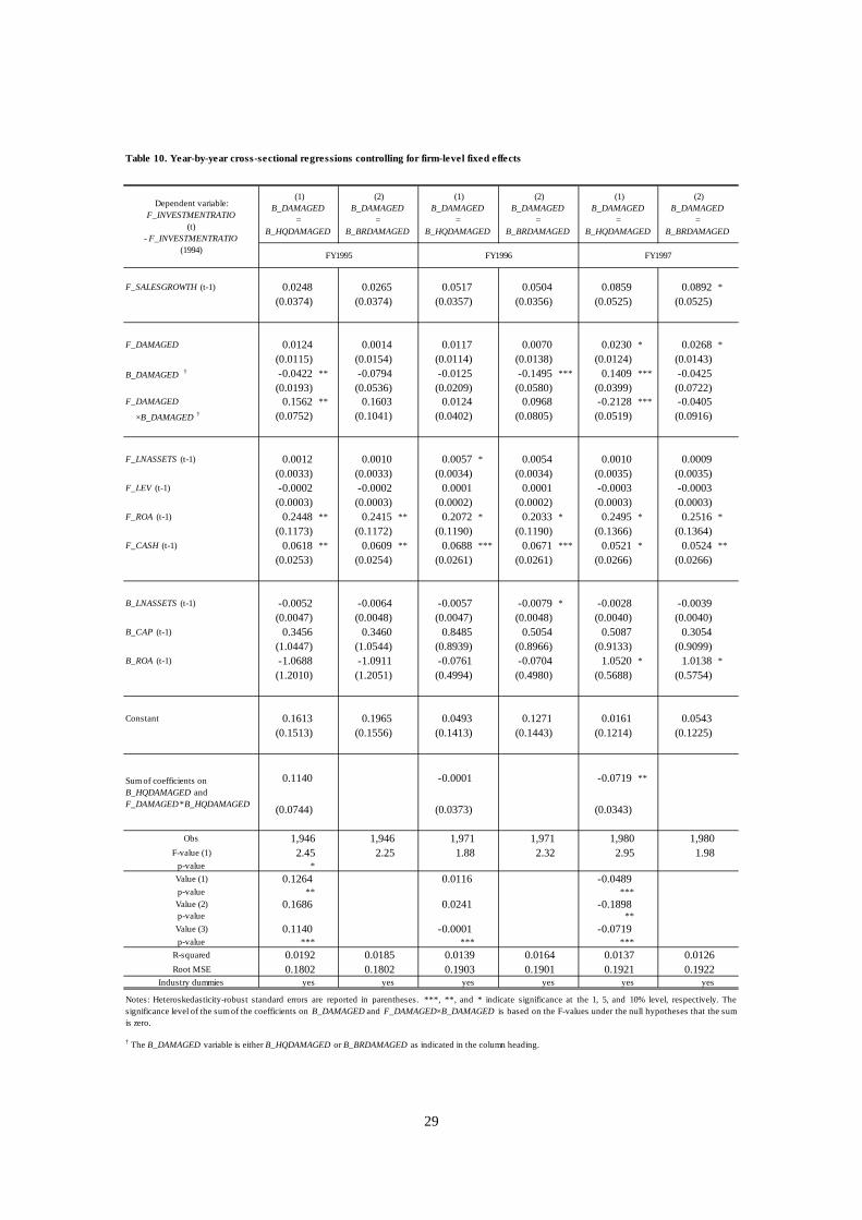
29
F_SALESGROWTH (t-1) 0.0248 0.0265 0.0517 0.0504 0.0859 0.0892 *
(0.0374) (0.0374) (0.0357) (0.0356) (0.0525) (0.0525)
F_DAMAGED 0.0124 0.0014 0.0117 0.0070 0.0230 * 0.0268 *
(0.0115) (0.0154) (0.0114) (0.0138) (0.0124) (0.0143) B_DAMAGED † -0.0422 ** -0.0794 -0.0125 -0.1495 *** 0.1409 *** -0.0425
(0.0193) (0.0536) (0.0209) (0.0580) (0.0399) (0.0722) F_DAMAGED 0.1562 ** 0.1603 0.0124 0.0968 -0.2128 *** -0.0405 ×B_DAMAGED † (0.0752) (0.1041) (0.0402) (0.0805) (0.0519) (0.0916)
F_LNASSETS (t-1) 0.0012 0.0010 0.0057 * 0.0054 0.0010 0.0009(0.0033) (0.0033) (0.0034) (0.0034) (0.0035) (0.0035)
F_LEV (t-1) -0.0002 -0.0002 0.0001 0.0001 -0.0003 -0.0003(0.0003) (0.0003) (0.0002) (0.0002) (0.0003) (0.0003)
F_ROA (t-1) 0.2448 ** 0.2415 ** 0.2072 * 0.2033 * 0.2495 * 0.2516 *
(0.1173) (0.1172) (0.1190) (0.1190) (0.1366) (0.1364) F_CASH (t-1) 0.0618 ** 0.0609 ** 0.0688 *** 0.0671 *** 0.0521 * 0.0524 **
(0.0253) (0.0254) (0.0261) (0.0261) (0.0266) (0.0266)
B_LNASSETS (t-1) -0.0052 -0.0064 -0.0057 -0.0079 * -0.0028 -0.0039(0.0047) (0.0048) (0.0047) (0.0048) (0.0040) (0.0040)
B_CAP (t-1) 0.3456 0.3460 0.8485 0.5054 0.5087 0.3054(1.0447) (1.0544) (0.8939) (0.8966) (0.9133) (0.9099)
B_ROA (t-1) -1.0688 -1.0911 -0.0761 -0.0704 1.0520 * 1.0138 *
(1.2010) (1.2051) (0.4994) (0.4980) (0.5688) (0.5754)
Constant 0.1613 0.1965 0.0493 0.1271 0.0161 0.0543(0.1513) (0.1556) (0.1413) (0.1443) (0.1214) (0.1225)
0.1140 -0.0001 -0.0719 **
(0.0744) (0.0373) (0.0343)
Obs 1,946 1,946 1,971 1,971 1,980 1,980F-value (1) 2.45 2.25 1.88 2.32 2.95 1.98
p-value *Value (1) 0.1264 0.0116 -0.0489p-value ** ***Value (2) 0.1686 0.0241 -0.1898p-value **Value (3) 0.1140 -0.0001 -0.0719p-value *** *** ***
R-squared 0.0192 0.0185 0.0139 0.0164 0.0137 0.0126Root MSE 0.1802 0.1802 0.1903 0.1901 0.1921 0.1922
Industry dummies yes yes yes yes yes yes
Notes: Heteroskedasticity-robust standard errors are reported in parentheses. ***, **, and * indicate significance at the 1, 5, and 10% level, respectively. Thesignificance level of the sum of the coefficients on B_DAMAGED and F_DAMAGED×B_DAMAGED is based on the F-values under the null hypotheses that the sumis zero.
† The B_DAMAGED variable is either B_HQDAMAGED or B_BRDAMAGED as indicated in the column heading.
Table 10. Year-by-year cross-sectional regressions controlling for firm-level fixed effects
(1)B_DAMAGED
=B_HQDAMAGED
(2)B_DAMAGED
=B_BRDAMAGED
(1)B_DAMAGED
=B_HQDAMAGED
(2)B_DAMAGED
=B_BRDAMAGED
(1)B_DAMAGED
=B_HQDAMAGED
(2)B_DAMAGED
=B_BRDAMAGED
Sum of coefficients onB_HQDAMAGED andF_DAMAGED *B_HQDAMAGED
Dependent variable:F_INVESTMENTRATIO
(t)- F_INVESTMENTRATIO
(1994) FY1995 FY1996 FY1997


