Synthesis and Modeling of Silver and Titanium dioxide
Nanoparticles by
Population Balance Equations
Dissertation
zur Erlangung des akademischen Grades
Doktoringenieurin
(Dr.-Ing.)
von: Yashodhan Pramod Gokhale
geboren am: 05. October 1981 in Pune, India
genehmigt durch die Fakultät für Verfahrens- und Systemtechnik
der Otto-von-Guericke-Universität Magdeburg
Gutachter: Prof. Dr.-Ing. habil Jürgen Tomas
Prof. Dr.-Ing. habil Andreas Seidel-Morgenstern
Eingereicht am: 30. November 2009
Promotionskolloquium: 23. March 2010
When you set out on your journey to Ithaca,
pray that the road is long,
full of adventure, full of knowledge.
The Lestrygonians and the Cyclops,
the angry Poseidon do not fear them:
You will never find such as these on your path,
if your thoughts remain lofty, if a fine
emotion touches your spirit and your body.
The Lestrygonians and the Cyclops,
the fierce Poseidon you will never encounter,
if you do not carry them within your soul,
if your soul does not set them up before you.
Pray that the road is long.
That the summer mornings are many, when,
with such pleasure, with such joy
you will enter ports seen for the first time;
stop at Phoenician markets,
and purchase fine merchandise,
mother-of-pearl and coral, amber and ebony,
and sensual perfumes of all kinds,
as many sensual perfumes as you can;
visit many Egyptian cities,
to learn and learn from scholars.
Always keep Ithaca in your mind.
To arrive there is your ultimate goal.
But do not hurry the voyage at all.
It is better to let it last for many years;
and to anchor at the island when you are old,
rich with all you have gained on the way,
not expecting that Ithaca will offer you riches.
Ithaca has given you the beautiful voyage.
Without her you would have never set out on the road.
She has nothing more to give you.
And if you find her poor, Ithaca has not deceived you.
Wise as you have become, with so much experience,
you must already have understood what Ithacas mean.
(I shall conclude my thoughts with a famous poem 'Ithaca' written by C.P. Cavafy (Keeley
and Sherrard 1992). The poem tells us that the final destination is always important, but it is
the journey with all its adventures that is more important and enjoyable.)
ITHACA
Ithaca

This work is dedicated to my beloved parents

Acknowledgments
Magdeburg and river Alba will always remain very close to my heart. They will remain special for the
friends they gave me, and ofcourse for the Otto-von Guericke University where I studied for the past
four years. The university not only opened doors to scientific research, but also broadened my views in
many aspects of the world. Many individuals provided support, help and encouragement during my
time in the graduate school. Now I would like to express my gratitude for them.
I am eternally thankful to Prof.-Dr. - Ing. habil. Jürgen Tomas, the best advisor one could find. Not
only did he teach me scientific thinking of the highest caliber but more importantly, he taught
me-through his own example-to be considerate, forthcoming, balanced and patient during interactions
with colleagues, teachers and students. His keenness about knowing the basics and about questioning
assumptions is an important lesson, which I shall carry with me throughout my career. He molded me
from being just a student to, hopefully, being a researcher. Besides being a good professor, he has
been a warm and cheerful person.
I am thankful for the financial support I received from the DFG-Graduiertenkolleg-828,”
Micro-Macro-Interactions in Structured Media and Particle Systems”, Otto-von-Guericke-Universität,
Magdeburg for this PhD program. I would like to thank Prof. Dr. Gerald Warnecke, and Prof. Dr.-Ing.
Albrecht Bertram for giving me valuable advice and also an opportunity to work in an
interdisciplinary project.
I would like to express my sincere and deep gratitude to Dr. rer. nat. Jitendra Kumar. His advice and
encouragement during the course of my research has been great help.
I am also very grateful to Dr. rer. nat. Werner Hintz who has shown considerable interest in my work.
Moreover, I value my scientific discussions during experimental work with Dipl.-Ing. Veselina
Yordanova. Also, I am thankful to Dr. rer. nat. Peter Veit for TEM micrographs and Dr. rer. nat.
Hartmut Heyse for SEM images. I would like to thank other members of the chair for their useful
comments and suggestions for the work included in this thesis. I have enjoyed working with Peter,
Martin, Sebastian, and Dipl.-Ing. Bernd Ebenau, and would appreciate their cooperation.
To Rajesh Kumar and Ankik Kumar; who deserve a special mention for sharing the triumphs with me.
They made me truly appreciate mathematics and left me with memories of hilarious and enlightening
moments to be treasured forever. I have thoroughly enjoyed all of our dinners, and delightful
conversations, which made our life in Magdeburg entertaining as well as memorable.

To the great writers and scientists who through their writings have provided me with immense
intellectual and moral inspiration; they have taught me more than I realize. Especially, I would like to
acknowledge the work and words of George Washington Carver and Richard Feynman. I have often
seen the world through their eyes, and I am sure they will continue to motivate me.
To all my friends in Magdeburg who provided support and encouragement to me during my stay here;
my heartfelt regards to all of them- Stan, Bhooshan, Rajesh,Vikrant, Bala, Ayan, Sagar, Yogesh,
Thiru, Reza, Chris, Katja, Maren, Penka, Marc, and Frau. Martina. They are truly wonderful people
who are now my family. I will always cherish the time I spent with them. To Alex, Thomas, Kai who
are my best friends outside the graduate school and with whom I spent many enjoyable weekends. I
also appreciate the support of friends-Chinmay, Harshada, Vikrant, Janhavi, Vivek,- and teachers from
far away Pune, India.
My special thanks to Dr. Aniket, Dr. Ashutosh and Ritwik; my long friendship with these dear friends
grew stronger in the course of my doctoral studies. I shall always owe them for the intellectually
stimulating, academic and non-academic discussions.
Most importantly, my deepest regard to the closest persons of my life who have given me all I could
ask for and much, much more that can ever be expressed in words; my family-Aai-Baba, grandparents
and brother Pushkaraj. I also want to thank my other parents, Mr. and Mrs. Deshpande for their
warmth and affection.
My mother and father are among the kindest and the most patient people I know. My grandfather had
one of the finest and the most intelligent scientific minds I have encountered. I will be eternally
indebted to him for constantly arousing in me a sense of curiosity and wonder about both the physical
and the human world.
Last but not the least; I would make a special mention of my soul mate, Ashwini-to whose opinion I
am addicted. Her kindness and grace, and her untiring contribution in reading, reading, and editing
every draft of this thesis, have been invaluable to me. Her presence has been my strength all through.
Abstract
The present scenario of well-controlled large-scale production of nanoparticles is a very
important aspect in nanotechnology. The present work aims at investigating different
engineering aspects of the production of silver and titanium dioxide nanoparticles using
different chemical methods. Eventually, this leads to possible process control. Silver and
Titania is one of the most extensively used materials for research, application and production
of nano size materials.
This thesis reports detailed synthesis of silver nanoparticles produced from the reduction of
silver nitrate by stabilizing and reducing agents. Silver nanoparticles have a strong tendency
to agglomerate. This reduces the surface to volume ratio and hence the resultant is the
catalytic effect. Silver nanoparticles are produced in the batch reactor at a different shear rate
and are investigated experimentally. Finally, the colloidal solution of capped silver
nanoparticles is free from agglomeration for several months.
To control the particle size and morphology of nanoparticles is of crucial importance from a
fundamental and also an industrial point of view. Titanium dioxide (TiO2) is one of the most
useful oxide materials, because of its widespread applications in photocatalysis, solar energy
conversion, sensors and optoelectronics. Controlling particle size and monodispersity of TiO2
nanoparticles is a challenging task. The control and prediction of these dynamics are based on
the conditions of the process and the nature of chemicals. This work discusses a new approach
for simultaneous agglomeration and disintegration of Titanium dioxide nanoparticles. The
precipitation of nanoparticles in the batch reactor is investigated experimentally at different
shear rates as well as by numerical simulations based on the population balance equations.
The population balance model for agglomeration and disintegration leads to a system of
integro-partial differential equations, which can be solved by several numerical methods. The
shear rate influences the particle size distributions.
This work also investigates the effect of the surface stabilization with varied surfactants on
the Titanium dioxide particles. The steric stabilization of polymer and various functional
groups of dispersants is also considered. The interaction between different particles greatly
affects both, the total energy potential and the stability ratio. Employing energy to the flow
field escalates the energy barrier in the colloidal system. Eventually this leads to lower
stability. Monodispersed spherical titania particles in the size range 10-100 nm are produced
in a sol-gel synthesis from titanium tetra-isopropoxide.
The silver and titania nanoparticles were characterized by dynamic light scattering, scanning
electron microscopy and transmission electron microscopy to determine particle size
distribution and shape. Also the specific surface area is measured by BET method.
The population balance model in this work is numerically solved by cell average technique.
The experimental results are compared with the simulation using different agglomeration and
disintegration kernels. It is found that the experimental results of the particle size distributions
at different shear rates of TiO2 are in good agreement with the simulation results. This
includes a comparison of the derived particle size distributions, moments and their accuracy
depending on the starting particle size distributions.
This study shows that particle sizes, morphology and monodispersity of colloidal particles of
silver and TiO2 can be controlled by two processes – one, by making appropriate choice of
stabilizing and reducing agents; two, by adding surfactants and polymers or salt during the
synthesis.
Zusammenfassung
Gegenwärtig stellt die gezielte Herstellung von Nanopartikeln im technischen Maßstab einen
wichtigen Forschungsgegenstand in der Nanotechnologie dar. Es werden verschiedene
ingenieurwissenschaftliche Aspekte zur Herstellung von Nanopartikeln aus Silber und
Titan(IV)-oxid mit Hilfe verschiedener Prozesse untersucht, mit dem Ziel, diese möglichst zu
steuern und zu kontrollieren. Dabei zählen insbesondere das Silber und das Titan(IV)-oxid zu
den am meisten untersuchten Stoffen hinsichtlich der Forschung, Produktion und Anwendung
nanoskaliger Materialien.
Die vorliegende Arbeit beschreibt im einzelnen die Herstellung von Nanopartikeln aus Silber
durch eine Reduktion von Silbernitrat unter Zusatz von Stabilisatoren und Reduktionsmitteln.
Silber-Nanopartikel zeigen dabei eine starke Tendenz zur Agglomeratbildung. Diese
verringert die spezifische Oberfläche und daraus resultierend die katalytische Wirkung der
Partikel. Die Herstellung der Silber-Nanopartikel erfolgte in einem Labor-Rührreaktor, die
Partikelbildung wurde experimentell bei unterschiedlichen Schergeschwindigkeiten
untersucht. Dabei ist es möglich, eine kolloidale Suspension aus stabilisierten Nanopartikeln
herzustellen, die für mehrere Monate stabil gegen Agglomeration ist.
Die Steuerung der Partikelgröße und der Morphologie der Nanopartikel ist von äußerster
Wichtigkeit, sowohl aus wissenschaftlicher als auch aus technischer Sicht. Titan(IV)-oxid
stellt eines der interessantesten Oxide auf Grund seiner Anwendung in der Photokatalyse,
Solarenergietechnologie, Optoelektronik und als Sensormaterial dar. Die Steuerung der
Partikelgröße und der Morphologie ist hierbei eine besondere Herausforderung. Grundlegend
sind für die Steuerung und Vorhersage der dieser dynamischen Prozesse einerseits die
Prozessparameter, andererseits die chemischen Eigenschaften des Stoffsystems. Die
vorliegende Arbeit diskutiert einen neuen Ansatz für die gleichzeitig ablaufende
Agglomerations- und Desintegrationsprozesse der Titan(IV)-oxid-Partikel. Die Fällung der
Nanopartikel wurde experimentell in einem Labor-Rührreaktor bei verschiedenen
Schergeschwindigkeiten untersucht und auf Basis von Populationsbilanzgleichungen
numerisch simuliert. Das Populationsbilanz-Modell für die Agglomerations- und
Desintegrationsprozesse führt zu einem System von Integro-Partial-Differentialgleichungen,
die mit Hilfe verschiedener numerischer Methoden gelöst wurden. Die Schergeschwindigkeit
beeinflußt die Partikelgrößenverteilungen.
Diese Arbeit untersucht außerdem die Wirkung der Oberflächenstabilisierung durch
unterschiedliche Tenside auf die Titan(IV)-oxid-Partikel. Die sterische Stabilisierung mit
Hilfe von Polymeren und Dispergierhilfsmitteln mit verschiedenen funktionellen Gruppen
wird ebenfalls betrachtet. Das Zusammenspiel zwischen verschiedenen Partikeln beeinflußt
wesentlich sowohl das Gesamtwechselwirkungspotential als auch den Stabilitätsfaktor. Indem
Energie dem Strömungsfeld zugeführt wird, kann die Energiebarriere im kolloidalen System
überwunden werden. Möglicherweise führt dies zu einer geringeren Stabilität.
Die mit Hilfe des Sol-Gel-Prozesses aus Tetraisopropyl-orthotitanat hergestellten
monodispersen kugelförmigen Titan(IV)-oxid-Partikel haben eine Größe zwischen 10 und
100 nm.
Die Nanopartikel aus Silber bzw. Titan(IV)-oxid wurden mittels dynamischer Lichtstreuung,
Raster- und Transmissionselektronenmikroskopie charakterisiert, um entsprechend die
Partikelgrößenverteilung und die Partikelform zu bestimmen. Die spezifische
Partikeloberfläche wurde mit Hilfe der BET-Methode erhalten.
Das Populationsbilanzmodell in dieser Arbeit wird numerisch auf Grundlage der sogenannten
Cell-Average-Methode gelöst. Die Ergebnisse der Simulationsrechnungen auf Basis der
Populationsgleichungen unter Verwendung unterschiedlicher Ansätze für die jeweiligen
Agglomerations- und Desintegrationskerne werden mit den experimentellen Ergebnissen
verglichen. Die experimentellen Partikelgrößenverteilungen können durch die
Simulationsergebnisse für verschiedene Schergeschwindigkeiten wiedergegeben werden. Das
beinhaltet einen Vergleich der berechneten Partikelgrößenverteilungen bzw. Momente sowie
deren Genauigkeit in Abhängigkeit von den am Beginn vorliegenden
Partikelgrößenverteilungen.
Die vorliegende Arbeit zeigt, dass die Partikelgröße, Morphologie und Monodispersität der
kolloidalen Partikel aus Silber bzw. Titan(IV)-oxid durch zwei Prozesse gesteuert werden
können, einerseits durch die geeignete Wahl von Stabilisatoren und Reduktionsmitteln,
andererseits durch den Zusatz von Tensiden, Polymeren oder Elektrolyten während des
Herstellungsprozesses.
Contents
Nomenclature ............................................................................................................................. 7
Greek Symbols ........................................................................................................................... 8
Chapter 1 .................................................................................................................................... 9
1 Nanoparticles, Motion and Life ....................................................................................... 10
1.1 Introduction ............................................................................................................... 10
1.2 Problem and Motivation ............................................................................................ 12
1.3 Outline of Contents .................................................................................................... 13
Chapter 2 .................................................................................................................................. 15
2 Fundamental Aspects ....................................................................................................... 16
2.1 Nano Scale Materials ................................................................................................. 16
2.2 Synthesis of Nano Materials ...................................................................................... 17
2.3 Different methods for synthesis of Silver and TiO2 nanoparticles ............................ 19
2.3.1 Synthesis of silver nanoparticles by different processes .................................... 19
2.3.2 Sol-gel synthesis ................................................................................................. 21
2.3.3 Synthesis of titanium dioxide nanoparticles by different methods .................... 22
2.3.4 Synthesis of Surfactant based nanoparticles by different methods .................... 24
2.4 Colloidal Particles...................................................................................................... 25
2.5 Interparticle Forces .................................................................................................... 26
2.5.1 Van der Waals Attraction Forces ....................................................................... 26
2.5.2 Electrostatic Repulsion Forces ........................................................................... 27
2.5.3 DLVO theory ...................................................................................................... 28
2.5.4 Steric Interaction ................................................................................................ 30
2.6 Colloidal Stabilization ............................................................................................... 30
2.6.1 Steric Stabilization ............................................................................................. 31
2.6.2 Electrostatic Stabilization ................................................................................... 31
2.6.3 Zeta Potential ...................................................................................................... 33
Chapter 3 .................................................................................................................................. 35
3 Characterization methods of Nanoparticles ..................................................................... 36
3.1 Particle Size Distribution ........................................................................................... 36
3.2 Dynamic Light Scattering- DLS ................................................................................ 38
3.2.1 Principle of Measurement .................................................................................. 39
3.2.2 Non-Invasive Back-Scatter (NIBS) .................................................................... 39
3.2.3 Operation of the Zetasizer Nano-Size measurements ........................................ 40

3.3 Low Angle Laser Light Scattering (LALLS) ............................................................ 42
3.4 Zeta Potential Measurement ...................................................................................... 43
3.4.1 Laser Doppler Electrophoresis ........................................................................... 43
3.4.2 Measuring Electrophoretical Mobility ............................................................... 44
3.4.3 Laser Doppler Velocimetry ................................................................................ 45
3.4.4 Operation of the Zetasizer Nano- Zeta potential measurements ........................ 45
3.5 Scanning Electron Microscope - SEM ...................................................................... 47
3.6 Transmission Electron Microscopy-TEM ................................................................. 49
Chapter 4 .................................................................................................................................. 52
4 Experimental Set up and Synthesis of Materials .............................................................. 53
4.1 Experimental Set up................................................................................................... 53
4.1.1 Types and Characteristics of Stirrer ................................................................... 53
4.1.2 Apparatus and Experimental Design .................................................................. 56
4.2 Silver nanoparticles synthesis .................................................................................... 57
4.2.1 Experimental Method for Silver ......................................................................... 58
4.2.1.1 Double reduction method for synthesis of silver nanoparticles .................. 58
4.2.1.2 Production of colloidal silver ...................................................................... 59
4.3 Titanium dioxide nanoparticles synthesis .................................................................. 62
4.3.1 Experimental method for Titanium dioxide ....................................................... 62
4.3.1.1 Sol-gel synthesis of TiO2 ............................................................................ 62
4.3.1.2 Surfactant based Titania nanoparticles ....................................................... 65
Chapter 5 .................................................................................................................................. 68
5 Population Balance Modeling .......................................................................................... 69
5.1 Introduction ............................................................................................................... 69
5.2 Recent survey ............................................................................................................ 70
5.3 Kinetics of the Simultaneous Agglomeration and Disintegration Sub-
Processes .............................................................................................................................. 73
5.3.1 Agglomeration Sub-Process .............................................................................. 73
5.3.2 Disintegration Sub-Process ................................................................................ 74
5.3.3 The Moment Form of the Population Balance ................................................... 75
5.4 Kernels of the Agglomeration and Disintegration Kinetics ...................................... 75
5.4.1 Agglomeration rate kernel ................................................................................. 75
5.4.2 Convection-Controlled Agglomeration .............................................................. 77
5.4.2.1 Laminar Flow .............................................................................................. 78

5.4.2.2 Turbulent Flow ............................................................................................ 79
5.4.3 Diffusion- Controlled Agglomeration ................................................................ 80
5.4.4 Relative Sedimentation ...................................................................................... 81
5.4.5 Effects of hydrodynamic interactions ................................................................ 82
5.4.6 Comparison of Agglomeration Kernels: ............................................................ 83
5.4.7 Disintegration rate kernel ................................................................................... 84
5.4.7.1 Austin Kernel .............................................................................................. 85
5.4.7.2 Diemer Kernel ............................................................................................. 85
5.4.8 Comparison of Disintegration Kernels ............................................................... 87
5.5 Methods to Solve the Population Balance Equations ................................................ 88
5.5.1 Numerical Methods ............................................................................................ 88
5.5.2 Cell Average Technique- CAT .......................................................................... 92
Chapter 6 .................................................................................................................................. 96
6 Experimental and Modeling Results ................................................................................ 97
6.1 Experimental results of silver nanoparticles .............................................................. 97
6.1.1 Effect of Capping Agent .................................................................................... 97
6.1.2 Effect of Reducing Agent ................................................................................. 100
6.1.3 Effect of Shear Rate on the particle size distribution ....................................... 102
6.1.4 Morphology and Particle Size Distribution ...................................................... 104
6.1.4.1 Scanning Electron Microscopy (SEM) ..................................................... 104
6.1.4.2 Transmission Electron Microscopy (TEM) .............................................. 106
6.2 Experiment and Modeling of Titanium dioxide nanoparticles ................................ 108
6.2.1 Simultaneous process of agglomeration-disintegration of titanium dioxide .... 108
6.2.1.1 Austin kernel and Shear kernel ................................................................. 109
6.2.1.2 Diemer Kernel and Shear kernel ............................................................... 112
6.2.1.3 Effect of Sum and Austin kernel on PSD ................................................. 114
6.2.1.4 Effect of Sum and Diemer kernel on PSD ................................................ 116
6.2.1.5 Effect of Process parameters on particle size distributions ...................... 118
6.2.2 Disintegration of Surfactant based Titanium dioxide ...................................... 126
6.2.2.1 Effects of Different Surfactants ................................................................ 126
Chapter 7 ................................................................................................................................ 132
7 Conclusions and Outlook ............................................................................................... 133
7.1 Conclusions ............................................................................................................. 133
7.2 Outlook .................................................................................................................... 135

Appendix ................................................................................................................................ 136
A. Shear Rate Calculation ................................................................................................... 136
B. Disintegration function from normalized cumulative disintegration ............................. 139
function. .................................................................................................................................. 139
Reference ................................................................................................................................ 142
Nomenclature 7
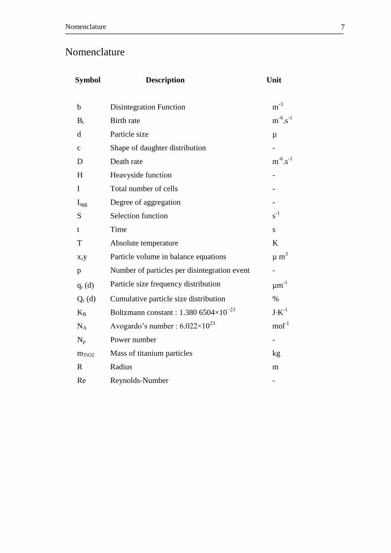
Nomenclature
Symbol Description Unit
b Disintegration Function m-3
Bi Birth rate m-6
.s-1
d Particle size µ
c Shape of daughter distribution -
D Death rate m-6
.s-1
H Heavyside function -
I Total number of cells -
Iagg Degree of aggregation -
S Selection function s-1
t Time s
T Absolute temperature K
x,y Particle volume in balance equations µ m3
p Number of particles per disintegration event -
qr (d) Particle size frequency distribution µm-1
Qr (d) Cumulative particle size distribution %
KB Boltzmann constant : 1.380 6504×10−23
J·K-1
NA Avogardo‟s number : 6.022×10²³
mol-1
Np Power number -
mTiO2 Mass of titanium particles kg
R Radius m
Re Reynolds-Number -

8
Greek Symbols
Symbol Description Unit
Collision frequency -
β One-dimensional agglomeration kernel m-3
. s-1
ε Turbulent energy dissipation rate m2. s
-3
F Density of the fluid kg. m-3
Kinematic viscosity of the fluid m2. s
-1
Viscosity of the fluid kg. m-1
. s-1
λ Wavelength m
ξ Zeta potential mV
κ Debye Hückel parameter nm-1
Shear rate s-1
x Particle volume fraction m3
Dimensionless material constant -
Dimensionless material constant -
Subscripts
agg Aggregation
disn Disintegration
break Breakage
nuc Nucleation
i; j Index
Acronyms
CAT Cell Average Technique
FPT Fixed Pivot Technique
ODE Ordinary Differential Equation
PBE Population Balance Equation
PSD Particle Size Distribution

9
Chapter 1
Nanoparticles, Motion and Life
“There are more things in heaven and earth, Horatio
Than are dreamt of in your philosophy”
- Hamlet, William Shakespeare
10
1 Nanoparticles, Motion and Life
1.1 Introduction
anoscience is a scientific effort towards achieving complete control over of atoms,
molecules and larger atomic structures including surfaces and bulk material. This
control at the most basic level does not, however, come without difficulty, and at this point
basic science is struggling to understand even the simplest building blocks and how they
interact. Once this understanding is secured, nanotechnology will be apt to affect every aspect
of human life, from the way we produce energy to the way we cure diseases. The basis of all
life is molecular motion. As the great physicist Richard Feynman (Feynman, Leighton et al.
1995) said
“If, in some cataclysm, all of scientific knowledge were to be destroyed, and only one
sentence passed on to the next generations of creatures, what statement would contain the
most information in the fewest words? I believe it is the atomic hypothesis (or the atomic fact,
whatever you wish to call it) that all things are made of atoms – little particles that move
around in perpetual motion, attracting each other when they are a little distance apart, but
repelling upon being squeezed into one another. In that one sentence, you will see, there is an
enormous amount of information about the world, if just a little imagination and thinking are
applied.”
Controlling the physical and chemical properties of materials requires detailed knowledge
about the behavior of the atoms and their interplay with other atoms in their surroundings. It
also requires materials that will allow the manipulations to result in a broad range of
properties. Metal oxides are proving to be a very interesting group of materials in this respect,
because they cover the entire range of properties available; some are high superconducting
while other are insulators, some are magnetic others not, and both their optical and
mechanical properties vary a great deal.
Nanoparticulate metal clusters/colloids are defined as isolable particles in the nanometer size
range, which are prevented from agglomeration by protecting shells. They can be redispersed
in water (hydrosols) or organic solvents (organosols). The number of potential applications of
these colloidal particles is growing rapidly because of the unique electronic structure of the
nanosized metal particles and their extremely large surface areas (J.Turkevich, P.C.Stevenson
et al. 1951). Highly dispersed mono and bimetallic colloids can be used as precursors for a
new type of catalyst that is applicable both, in the homogeneous and heterogeneous phases
N

11
(Schmid. 1996). Nanoparticles, comprised of one or two different metal elements, are of
considerable interest from both the scientific and technological points of view (Rodriguez and
Goodman 2002).
Many efforts have been made to develope appropriate processes to prepare silver and titania
nanoparticles for generating colloidal particles due to their technological importance. Silver
nanoparticles and titanium oxide particle coating is a very important material due to its
multifunctional application in solar cells, anti-reflective optical coatings, hydrophobic
materials, photochromic and electrochromic devices, gas sensors, biosensors, corrosion
protection, bactericides, optical devices, among others (Daoud and Xin 2004; Toma, Bertrand
et al. 2006)
One of the fundamental issues that need to be addressed in modeling macroscopic mechanical
behavior of nano-structured materials based on molecular structure is the large difference in
length scales. On the opposite end of the length scale, the spectrum of computational
chemistry and solid mechanics consists of highly developed and reliable modeling methods.
Computational chemistry models predict molecular properties based on known quantum
interactions, while computational solid mechanics models predict the macroscopic mechanical
behavior of materials idealized as continuous media based on known bulk material properties.
However, a corresponding model does not exist in the intermediate length scale range. If a
hierarchical approach is used to model the macroscopic behavior of nano-structured materials,
then a methodology must be developed to link the molecular structure and macroscopic
properties.
Many properties of solid particles are not only a function of the material‟s bulk properties but
also depend on the particle size distribution (PSD). These property changes arise from the
increasing influence of surface properties in comparison to volumetric bulk properties as the
particle size decreases. Especially nanoscaled particles show altered properties and have
therefore widespread applications like pigments, pharmaceuticals, cosmetics, ceramics,
catalysts and filling materials. Since the desired product properties might vary with particle
size as well as with the degree of aggregation or the aggregate structure, controlling of the
PSD and the aggregate structure is a key criterion for product quality. New and improved
products can then be designed by adjusting and optimizing the PSD and the particle structure.
Precipitation is a promising method for the economic production of commercial quantities of
nanoparticles as it is fast and operable at an ambient temperature. However, process control
due to the rapidity of the involved sub-processes and especially to prevent aggregation
through stabilization represents a challenge.

12
To control these sub-processes, balance models are used in particle technology. Population
balances for agglomeration and disintegration appear in a wide range of applications
including nano-technology, granulation, crystallization, atmospheric science, physics and
pharmaceutical industries. There are several numerical methods such as Monte Carlo, finite
element, finite volume, sectional approaches to solve the agglomeration and disintegration
population balance equations (Israelachvili 1985; F. Einar Kruis, Arkadi Maisels et al. 2000).
1.2 Problem and Motivation
In recent times, oxide and noble materials have attracted special attention and a lot of
research is concentrated on the synthesis of silver and titania nanoparticles by various
techniques. The objective of this work is to synthesize silver nanoparticles by means of
chemical double reduction method with further stabilization by means of capping agents
utilizing different long chain acid. Silver nanoparticles are also made in the liquid phase using
reducing agents on a laboratory scale. This technology has several advantages over
conventional methods. Nano-sized particles especially those less than fifty nanometers (50
nm) are receiving significant attention in industries. Numerous industries apply nano-scale
materials in their operations.
The objective of the thesis is to study the agglomeration and disintegration process of TiO2
nanoparticles by using sol-gel synthesis. Also it is important to study the effect of parameters
like stirrer speeds, electrolyte solution, and pH during agglomeration and disintegration
kinetics of titanium dioxide nanoparticles. Characterization of diffusion driven disintegration
process was taken from the particle size distributions measured in the dynamic light scattering
and low angle laser light scattering in order to follow the agglomeration and redispersion
kinetics. The experimental results have been used for simulation by the mathematic modeling.
The population balance model for agglomeration disintegration leads to a system of
integro-partial differential equations which is numerically solved by the cell average
technique. This includes a comparison of the derived particle size distributions, moments and
its accuracy depending on the starting particle size distribution. The experimental results are
also compared with the simulation using different agglomeration and disintegration kernels.
In this thesis, we investigate the synthesis of surface stabilized TiO2 nanoparticles with
different surfactants. The steric stabilization of the polymer and various functional groups of
dispersants are also considered. The influence of various precursor concentrations and
different surfactants on the particle size distribution is investigated. The population balance

13
model for disintegration process is numerically solved by the cell average technique. The
experimental results are also compared with the simulation using two different disintegration
kernels.
The goal was to contribute to the understanding of the modeling to improve the yield and
quality of products and the scale up of new processes from a laboratory scale level to an
industrial level. In both the cases the model needs to capture the important physico-chemical
parameters of the formation of nanoparticles, their interactions with each other. This requires
detailed models of the chemical reactions, the population of particles and for the mostly
thermodynamics of the reaction.
There are three main reasons why sizes of nanoparticles matter so much one, they have a very
high surface area, which makes nanoparticles very suitable for catalytic reaction, drug
delivery and energy storage. Two have higher surface tension and local electromagnetic
effects, which makes it harder and less brittle compare to larger size of material. Three, could
be manipulated on the fundamental properties of materials without changing the chemical
composition. Based on the fact above one could say that materials can be engineered. New
properties of materials that may exist but have not been found in nature may emerge because
of the manipulation. Combination between nanoparticles, its technologies, and other science
leads to a revolutionary invention.
1.3 Outline of Contents
This research mainly includes two parts; the first is synthesis of silver and titanium dioxide
nanoparticles by different chemical methods. In the second part, we develop population
balance model for titanium dioxide nanoparticles by using different reaction parameters. The
outline of the proposed research is organized as follows.
In total, there are seven chapters included in this thesis work. Chapter one will introduce the
readers to the enormous and booming phenomena of nanoparticles and its technology used
recently. All the basic knowledge concerning nanoparticles such as available methods of
production and the chemistry behind interaction of particles will be reviewed in chapter two.
In Chapter 3 deals with the different experimental techniques that are used extensively for
characterization of the oxide and noble materials. It contains information about related
measurement apparatuses commonly used for characterizing nanoparticles.
Chapter four, provides information about the materials, the experimental set-up, and synthesis
of silver and titanium nanoparticles by different techniques. First we give synthesis of silver
14
nanoparticles by chemical double reduction method. The second part gives a synthesis of
titanium dioxide nanoparticles by sol-gel method. It also discusses the synthesis of surface
stabilized TiO2 nanoparticles with different surfactants. The author will explain the purposes
of selecting such a condition and the kind of variation made for generating nanoparticles. This
is very important since it will gives a apply for all of the experiments.
Chapter 5 gives a brief overview of simulation methods for solving population balance
equations. Section 5.3 particularly focuses on the mathematical model and the existing
schemes for solving aggregation and disintegration equations. Further we present the different
agglomeration and disintegration kernels (section 5.4) which we use as the building block for
population balance model. Furthermore, the idea of solving population balance equations by
using different numerical methods is discussed in section 5.5. The newly developed sectional
numerical scheme as cell average technique has been summarized in section 5.5.2.
Results and discussion regarding the optimum shear rates for generating the smallest silver
and titanium dioxide nanoparticles and surface stabilized TiO2 nanoparticles will be discussed
in chapter 6. Numerically derived results from a population balance model that accounts for
agglomeration and disintegration are in good agreement with experimental observations. At
the end of this work, concluding remarks are given in chapter 7. Finally, some future
developments for improving the nano process design are pointed out.
At the end of the thesis we put two Appendixes. Appendix A gives all shear rate calculations
used in this work. Some more mathematical formulation for disintegration kernel is presented
in Appendix B.
15
Chapter 2
Fundamental Aspects
“So far as it goes, a small thing may give analogy of great things, and show the tracks of
knowledge.”
-The philosopher Lucretius

16
2 Fundamental Aspects
2.1 Nano Scale Materials
anoscale materials can be defined as those whose characteristic length scale lies within
the nanometric range i.e. between one to hundred of nanometer. Within this length scale,
the properties of matter are sufficiently different from individual atoms or molecules, and
bulk materials. The idea of manipulating and positioning individual atoms and molecules is
still new.
On 29th December 1959, Nobel laureate Prof. Richard Feynman gave an illuminating talk on
nano technology. It was entitled „There‟s Plenty of Room at the Bottom‟. Prof. Feynman said,
"The principles of physics, as far as I can see, do not speak against the possibility of
maneuvering things atom by atom. It is not an attempt to violate any laws; it is something, in
principle, that can be done; but in practice, it has not been done because we are too big."
In future, nanotechnology will help to assemble these atoms or these building blocks to give
new products. We will be able to put together the fundamental building blocks of nature
easily, inexpensively, and in most of the ways permitted by the laws of physics.
The properties of materials change as their size approaches to nanoscale and as the percentage
of atoms at the surface of a material becomes significant. Size dependent properties of
nanomaterials include quantum confinement in semiconductor particles, surface plasmon
resonance in some metal particles and super-para-magnetism in magnetic materials. Materials
reduced to nanoscale can suddenly show very different properties compared to what they
exhibit on macroscale, enabling unique applications. For instance; inert materials become
catalysts (platinum), solids turn into liquids at room temperature (gold), and insulators
become conductors (silicon).
A unique aspect of nanotechnology is the vast increase in ratio of surface to volume present in
many nanoscale materials which opens new possibilities in surface based science, such as
catalysis. Hence they have enhanced chemical, mechanical, optical and magnetic properties,
and this can be exploited for a variety of structural and non-structural applications.
Nanoparticles represent metastable clusters exhibiting the fundamental property to aggregate.
Thus, the stabilization of the nanoparticles may be accomplished by the capping of the
nanoparticles with weak electrostatically bound ions (Schmid 1994), by molecular ligands
(Green and OBrien 2000), micellar assemblies and different surfactants (Cole, Shull et al.
1999). The association of ligands to growing nanoparticles can control the dimensions and
N
17
shape of the nanocrystals (Pileni, Gulik-Krzywicki et al. 1998). Nanotechnology uses
knowledge from chemistry, physics and biology, and more specifically it is concerned with
observing atoms and molecules and manipulating them through visual observations at the
nanoscale level. A blend of nanoparticles, technology, and other sciences leads to a
revolutionary invention.
2.2 Synthesis of Nano Materials
We can synthesize nanoparticles by two different methods: by downscaling i.e. by making
things smaller, and by upscaling i.e. by constructing things from small building blocks. The
first method is called “top-down”, and the second method is called “bottom-up” approach.
The top-down approach follows the general trend of the microelectronic industry towards
miniaturization of integrated semi-conductor circuits. The lithographic techniques (top-down)
offer the connection between structure and technical environment. Top-down approach
involves typical solid-state processing of the materials. These methods are based on the
reduction of bulk (micro) sized materials into the nano-scale. High energy ball milling or
microfluidizers are used to break down dispersed solids to 100 nm. Coarse-grained materials
(metals, ceramic, and polymers) in the form of powders are crushed mechanically in ball
milling by hard materials such as steel or tungsten carbide. This repeated deformation due to
applied forces can cause large reduction in grain size since energy is being continuously
pumped into crystalline structures to create lattice defects. However, this approach is not
suitable for preparing uniformly shaped materials, and it is very difficult to realize very small
particles even with high energy consumption.
The bottom-up approach is based on molecular recognition and chemical self-assembly of
molecules. Bottom-up routes are more often used for preparing most of the nano-scale
materials with an ability to generate uniform size, shape, and distribution. Bottom-up routes
effectively cover chemical synthesis and the precisely controlled deposition and growth of
materials. In the bottom-up route, physical/aerosol and wet/chemical synthesis are widely
used for nanoparticles generation. There are several processes for synthesis of nanoparticles.
Mechanochemical processing is one of the processes known in particle technology. It uses
energy from dry milling to induce chemical reactions during ball powder collisions. This
process is still under development and rarely used because of its high energy demands. By
forming additional dilutes, the agglomeration of particles can be minimized by encapsulating
the particles (Komarneni 2003). Microemulsion techniques for nanoparticles synthesis are
18
becoming a new focus in this study of nano-scale materials. The principle of micro-emulsion
process is to conduct production of nanoparticles inside nanosized reactor. The reactors are so
small in a way that particles cannot grow large. A descriptive example would be interactions
between water and surfactant inside hydrocarbon solvent. Surfactant is an amphiphilic
molecule (has two distinct regions) with hydrophobic tail and hydrophilic head. The head
tends to gather with water and leave its tails encircled by solvent. This course of action will
disperse water into very small droplets, which react as nano reactors. The use of
microemulsion systems is introduced to precipitate BaSO4 nanoparticles, which shows the
ability for efficient control of particle properties (Qi, Ma et al. 1996; Li and Mann 2000;
Summers, Eastoe et al. 2002; Adityawarman, Voigt et al. 2005) .
The term „Aerosol‟ defined as the suspension of very fine particles of solids or droplets of
liquid in a gaseous medium. The medium acts to restrain the motion of random particles, and
support the particles against gravity energy (Reist 1993). Aerosol processes like flame
hydrolysis, spray pyrolysis and plasma synthesis which are mostly useful to produced carbon
black are well established for industrial scale, despite very high energy demands (U.Schubert
and Hüsing 2000).
Chemical/wet syntheses include classical crystallization, bulk or emulsion precipitation.
Sol-gel methods are widely used for fine chemical preparation. These routes involve the
reaction of chemical reactants with other reactants in either an aqueous or non-aqueous
solution. These chemical reactants react and self-assemble to produce a supersaturated
solution with the product. This supersaturated solution at certain conditions results in
particle nucleation. These initial nuclei then grow into nanometer size particles. Chemical
precipitation can be held in room temperature, by simply adding reducing agent to a metal salt
solution in order to precipitate out fine particles (Brinker and Scherer 1990; Yang, Zhang et
al. 2006). This process is inevitable of contaminants, either from excess of reactants (caused
by incomplete reaction due to low temperatures) or from reducing agent. Removal of those
impurities will lead to another problem. The phenomena that usually take place are
nucleation, crystal growth, agglomeration, and disintegration. These phenomena need to be
controlled to get desired sizes, shapes and morphology of the particles. As a result various
synthesis methods aim towards manufacturing materials for diverse products with new
functionalities at the nanoscale.
19
2.3 Different methods for synthesis of Silver and TiO2 nanoparticles
2.3.1 Synthesis of silver nanoparticles by different processes
With infinite applications in almost every field, nanotechnology is growing and becoming
popular in academia and industry. Nanomaterials have attracted considerable interest due to
their peculiar characteristics such as optical, mechanical, electronic and magnetic properties.
The synthesis of noble metal nanoparticles has been a subject of numerous applications.
Over the last decades silver has been engineered into nanoparticles, structures from 1 to 100
nm in size. Owing to their small size, the total surface area of the nanoparticles is maximized,
leading to the highest value of the activity to weight ratio. The ancient Greek and Roman
civilizations used silver vessels to keep water potable. Since the nineteenth century, silver
based compounds have been used widely in bactericidal applications in healing of burns and
also in wound therapy (H.Klasen 2000).
Furthermore, currently a diverse range of consumer products contain silver nanoparticles.
These products contain antibacterial/antifungal agents. Few examples of such products are air
sanitizer, respirators, wet wipes, detergents, soaps, shampoos, toothpastes, air filters, coatings
of refrigerators, vacuum cleaners, washing machines, food storage containers, cellular phones
etc (Buzea 2007). The silver particles in nano-scale exhibit high-antibacterial activity and
have no intolerable cytotoxic effects for human beings. The antibacterial effect has been
tested for yeast and E. coli by (Kim, Kuk et al. 2007). The experimental results showed that
the growth inhibition effect of silver nanoparticles was in a concentration-dependent manner.
They concluded that the silver nanoparticles were applicable to diverse medical devices and
antimicrobial systems.
A number of methods have been used in the past decades for preparing these noble silver
nanoparticles. The methods are as follows:-
1. This include condensation in vapour phase (Stabel, Eichhorst-Gerner et al. 1998),
chemical vapour deposition (CVD) or electrostatic spraying on solid substrate
(Okumura, Tsubota et al. 1998), ultrasound-induced reduction in solutions or reverse
micelles (Ji, Chen et al. 1999), and thermal decompositions of precursors in solvents,
and polymer films (Lidia Armelao, Renzo Bertoncello et al. 1997; Yanagihara, Uchida
et al. 1999).
2. The particles were mainly generated by reduction, and stabilized by various methods
(Brust, Walker et al. 1994; Jana, Wang et al. 2000; Jin, Cao et al. 2001). Silver

20
nanoparticles can be prepared by using a variety of reducing agents including
dimethylformamide and ethylene glycol (D.G.Duff, A.Baiker et al. 1993; K.S.Chou
and C.Y.Ren 2000). Silver nano wire and nano-prism have been reported by use of
silver nitrate in polyvinylpyrrolidone-PVP in N,N-dimethylformamide-DMF
(Pastoriza-Santos and Liz-Marzan 2002).
3. Large scale synthesis of capped or coated silver particles by solution method remains
highly challenging thus less attempted by the researchers. Citrate method for such
preparation has been widely utilized for aqueous colloidal solution of silver and gold
(J.Turkevich, P.C.Stevenson et al. 1951). The varieties are now available for
producing silver nanoparticles as stable, colloidal dispersions in water or organic
solvents (Brown and Hutchison 1999; Wang, Chen et al. 1999).
4. Most synthesis describes the use of suitable surface capping agents in addition to the
reducing agents for synthesis of nano-particles. Frequent use of organic compounds as
well as polymers has been described for obtaining re-dispersible nano-particles. It has
been observed that the size, morphology, stability, and chemical and physical
properties of silver nanoparticles have a strong dependence on the specificity of the
preparation method and experimental conditions.
5. Usually when metal nanoparticles are prepared by chemical methods, the metal ions
are reduced by the reducing agents, and protective agents or phase transfer agents are
added to stabilize the nanoparticles. In this, starch was used as the protecting agent,
and glucose was used as the reducing agent. Protecting agents retard the particle
growth and/or prevent agglomeration due to steric stabilization. Other (Chou and Ren
2000; Raveendran, Fu et al. 2003) uses polyvinyl alcohol and starch as protecting
agents. Silver nanoparticles act as catalyst, and these catalytic properties of silver
nanoparticles are supported on silica spheres (Jiang, Liu et al. 2005). The synthesis of
silver was conducted using spinning disk reactor (Tai, Wang et al. 2009).
6. Hydrogels or macroscopic gels have been used as promising templates or nanopots to
prepare silver nanoparticles. The available free-network space between hydrogel
networks reserves to grow and stabilize the nanoparticles (Vimala, Samba Sivudu et
al. 2009). Also the use of methanolic solution of sodium borohydride in tetrazolium
based ionic liquid leads to pure phase of silver nanoparticles (Singh, Kumari et al.
2009).
7. Biomolecules as reductants are found to have significant advantage over their
counterparts as protecting agents. It has been shown that extracellularly produced
21
silver nanoparticles using (Fusarium oxysporum) a naturally occurring edible
mushroom can be incorporated in several kinds of materials including clothes (Philip
2009). Amongst the many synthesis methods, surfactants and carboxylic acids have
found special mention for their ease in handling, effective capping, mild reducing
ability and human friendly nature.
2.3.2 Sol-gel synthesis
Sol-gel method is one of the most successful techniques for preparing nanosized metallic
oxide materials with high photocatalytic activities. By tailoring the chemical structure of
primary precursor and carefully controlling the processing variables, nanocrystalline products
with very high level of chemical purity can be achieved.
Sols and gels were two forms of matter which have already existed naturally for hundreds of
years. In 1846, Ebelmen synthesized first silica gels from silicon tetrachloride and alcohols,
followed by Faraday who synthesized sols from gold in 1853 (Pierre 1998). Sol is defined as
stable suspensions of solid particles in liquid solvents where gravity force is negligible. Gel is
a porous of three dimensionally interconnected solid networks that expand throughout its
medium.
Sol-gel processes a mixture of two or more solutions to start the chemical reactions namely
hydrolysis and condensation. During hydrolysis the metal alkoxide M-OR is broken down by
water molecules, and one or more alkoxide groups are replaced by hydroxide groups. It is
known that the hydrolysis rate of a metal alkoxide decreases with increase in the size of the
alkyl group (e.g., ethoxide, propoxide, butoxide) as a consequence of the positive partial
charge of the metal atom, which decreases with alkyl chain length, as shown by (Babonneau,
Sanchez et al. 1988; Kallala, Sanchez et al. 1992; Barboux-Doeuff and Sanchez 1994).
During condensation, water or alcohol molecules are eliminated through different
mechanisms (i.e. alkoxolation, oxolation, polycondensation, etc.) and oxygen bridges are
formed between metal atoms. The process is also described in terms of a particle formation
step, controlled by nucleation and molecular growth, and a subsequent agglomeration step,
where already formed particles collide and stick together. The relative rates of these processes
are very important since they determine the characteristics of the final product, such as
particle size distribution (PSD) and morphology, as well as the overall particulate structure
(e.g., sol versus gel).

22
The Sol-gel synthesis of titania nanoparticles consists of two-step process viz, hydrolysis and
polycondensation. Moreover, redispersion of titanium oxide (gel) to nano-titanium oxide (sol)
also takes place.
2.3.3 Synthesis of titanium dioxide nanoparticles by different methods
Titanium dioxide has received great attention due to its unique photocatalytic activity in the
treatment of environmental contamination. But for practical application, the photocatalytic
activity of TiO2 needs further improvement. An efficient way to improve the TiO2
photoactivity is to introduce foreign metal ions (surface modifications) into TiO2, which is
also called heterogeneous photocatalysis.
The sol-gel process is the most attractive method to introduce foreign metal ions into TiO2
powders and films. Several different methods have been developed for generating titania
nanoparticles. Following are the methods:
1. Titania particles are often synthesized in industries by digesting ore ilmenite with
sulfuric acid, followed by thermal hydrolysis of Titanium (IV)-ions in a highly acidic
solution and eventually carrying out a dehydration of the Titanium (IV) hydrous oxide
(X. Jiang, T. Herricks et al. 2003). The particles obtained with this method are often
irregular in shape and exhibit broad distribution in size. Recently, several techniques
have been reported for synthesizing monodispersed powders through controlled
nucleation and growth processes in dilute Titan(IV)-oxide solutions (Masaru
Yoshinaka, Ken Hirota et al. 1997; Jean and Ring 2002).
2. The most common procedures have been based on the hydrolysis of acidic solutions of
titanium (iv) salts, gas-phase oxidation reactions of TiCl4 (Matijevic, Budnik et al.
1977) and hydrolysis reactions of titanium alkoxide (Jean and Ring 2002) . However,
powders produced by these methods have generally lacked the properties of uniform
size, shape and unagglomerated state desired.
3. Monodispersed spherical titania oxide particles were prepared by controlled
hydrolysis of titanium tetraethoxide in ethanol (Eiden-Assmann, Widoniak et al.
2003). In some cases, the titania nanoparticles can be made by reaction in aerosols
(Salmon and Matijevic 1990; Park and Burlitch 2002). The TiO2 aerogels were
obtained by using a supercritical drying gel method(Novak, Knez et al. 2001).
4. Using a variation of this approach, (Yaacov Almog, Shimon Reich et al. 1982) have
successfully prepared monodispersed polymer particles in the range of 1-6 microns.

23
Their method involves the use of a polymeric steric stabilizer in combination with a
quaternary ammonium salt which, the authors claimed acts as an electrostatic
co-stabilizer. Production of titania particles from an alcoholic solution of titanium tetra
alkoxide using an amine-containing additive and water to hydrolyze said titanium
alkoxide solution is another alternative method (Olson and Liss 1989).
5. Another approach to preparing micron size particles is by dispersion polymerization.
This method has been very thoroughly reviewed by (Barrett 1997) and it has been
shown to produce particles with a very narrow size distribution. The process involves
the polymerization of a monomer dissolved in a medium in the presence of a graft
copolymer dispersant (or its precursor) to produce insoluble polymer dispersed in the
medium.
6. The TiO2 occurs in three different crystalline polymorphs: rutile (tetragonal), anatase
(tetragonal), and brookite (orthorhombic). These phases of TiO2 has been studied
widely because of its potential applications mainly in photoelectric conversion in solar
cells (O'Regan and Gratzel 1991; Bach, Lupo et al. 1998). The dye-sensitized TiO2
was used for solar energy conversion in photoelectrochemical cells (Nazeeruddin, Kay
et al. 2002).
7. Several works have been carried out for the synthesis of TiO2 nanoparticles, such as
microemulsion-mediated hydrothermal (Wu, Long et al. 1999), hydrothermal
crystallization(Yang and Gao 2005; Zhu, Lan et al. 2005).
8. Hydrothermal synthesis is a soft solution for chemical processing which provides an
easy route to prepare a well-crystalline oxide under the moderate reaction condition,
i.e. low temperature and short reaction time (Pookmanee, Rujijanagul et al. 2004). By
switching to sol-gel precursors with significant lower hydrolysis rate, it is possible to
produce titania spherical colloids with narrow distribution in size. Spherical
monodispersed particles have been synthesized in this regard by using a precursor,
Ti(OPr)3 (acac), derived from the modification of Ti(OPr)4 with acetyl acetone (acac)
(X. Jiang, T. Herricks et al. 2003).
The sol-gel technique offers some advantages compared to other solution methods, and is
therefore discussed in detail in the next sections.

24
2.3.4 Synthesis of Surfactant based nanoparticles by different methods
Surfactants are molecules that consist of hydrophobic and hydrophilic parts. Their
amphiphilic nature makes them surface active and, adsorbed at the oil/water interface, they
can reduce the bare oil-water interfacial tension to very low values. The hydrophilic end is
water soluble and is a polar or ionic group. The hydrophobic end is water-insoluble and can
be either a hydrocarbon chain or silicone. This dual functionality is the source of the surface
activity. The activity is due in large part to the unique structure of water. Because of this
property, surfactants are used in many practical applications ranging from crude oil recovery
to drug delivery and are also of scientificfic interest. Different methods have been developed
for generating surfactant based oxide nanoparticles. Listed below are the methods:-
1. Polymeric adsorption may serve as an effective way for modifying the surface of
nanoparticles and hence improving the stability of the suspension against flocculation.
Previously, the adsorption of polymers such as poly(vinylpyrrolidone) (PVP),
poly(ethylene glycol) (PEG), poly(vinyl alcohol) (PVA), and poly(ethylene oxide)
(PEO) on the surface of some metal oxide powders (TiO2, Fe3O4 and Al2O3) in
aqueous suspension was investigated (Lakhwani and Rahaman 1999; Chibowski,
Paszkiewicz et al. 2000).
2. The control of the surface properties of nanoparticles is of great importance. (Liufu,
Xiao et al. 2004) investigated the influence of PEG adsorption on the surface of ZnO
nanoparticles. ZnO nanocomposities can be prepared by a novel pickering emulsion
route using polyaniline (He 2004).
3. Specifically, the adsorption of polymeric additives onto the surface of the metal oxide
is ascribed to a combination of chemical and electrostatic interaction, hydrogen
bonding and Van Der Waals force (Zhang, Tang et al. 2003). For nonionic polymer,
hydrogen bonding is the primary adsorption mechanism. One is performed through
surface absorption or reaction with small molecules, such as the stearic acid, the
surfactant C18H37O (CH2CH2O)10H etc.(Ma, Zhang et al. 2003; Zhang, Tang et al.
2003).
4. Another method is based on grafting polymer chain onto the surface of nanoparticles
by covalently bonding to the hydroxyl groups existing on the particles(Gu, Onishi et
al. 2004) . In contrast, the advantage of the second method over the first one is due to
the fact that the properties of the polymer-grafted nanoparticles can be tailored

25
through a proper selection of the species of the grafting monomers and the grafting
conditions (Rong, Ji et al. 2002).
In the next section we will see the fundamentals of colloidal particles.
2.4 Colloidal Particles
Colloid science is generally understood to be the study of systems containing kinetic units
which are large in comparison with atomic dimensions (E.J.W.Verwey and Overbeck 1948).
It can be stated that the size of particles in the colloidal range is between 10 and 10,000 Å
units approx. In other words, colloidal particles are those with a size (or with one dimension)
between 1 nm and 1 µm. In this particle size range, i.e. 1 nm to 1 µm the particle interactions
are dominated by short-range forces, such as van der Waals attraction and surface forces. On
this basis the International Union of Pure and Applied Chemistry (IUPAC) suggested that a
colloidal dispersion should be defined as a system in which particles of colloidal size (1–1000
nm) of any nature (solid, liquid, or gas) are dispersed in a continuous phase of a different
composition (Everett 1971). Considering the size of the constituent atoms, this means that
colloidal particles are made of associations or colonies of approximately 103
to 109 atoms.
These atoms can be arranged in a crystalline or in an amorphous structure.
Colloid systems are mostly based on very small particles dispersed in a solution. There are
many important properties of colloidal systems that are determined directly or indirectly by
the interaction forces between particles. These colloidal forces consist of the electrical double
layer, van der Waals (attraction), Born (repulsion), hydration, and steric forces (repulsion).
Colloidal particles are dominated by surface properties. Hence it is sometimes said that
colloidal properties are those of a large surface concentrated in a small volume (Fisher,
Garcia-Rubio et al. 1998).
Colloidal particles are commonly found distributed as a separate phase; the disperse phase,
into another substance or substances; the dispersant or continuous phase. In this sense,
colloidal systems are heterogeneous material systems. Either of the two phases can be in any
of the states of matter: solid, liquid, or gas. The colloidal particles are designed by considering
various criteria related to the targeted applications such as particle size distribution, surface
polarity, surface reactive groups, and hydrophilic-hydrophobic balance of the surfaces.

26
ri rj
d
2.5 Interparticle Forces
There are three types of intermolecular forces acting between molecules in the colloidal
system. Those forces are van der Waals attraction forces, electrostatic repulsion forces, and
steric interaction. Together these three forces are used to control the agglomeration and
disintegration in our particulate systems as following.
2.5.1 Van der Waals Attraction Forces
The existence of a general attractive interaction between neutral atoms was first postulated by
Van der Waals in 1873, to account for certain anomalous phenomena occurring in non-ideal
gases and liquids. When nanoparticles are dispersed in a solvent, van der Waals attraction
force and Brownian motion play an important role. The influence of gravity becomes
negligible in this case. In this Thesis, special emphasis is laid on nanoparticles, although
particles in micrometer sizes have similar characteristics. In addition, we will focus on
spherical nanoparticles. Van der Waals forces are weak forces and become significant only at
a very short distance. Brownian motion ensures that the nanoparticles collide with each other
all the time. The combination of van der Waals attraction force and Brownian motion would
result in the agglomeration and disintegration of the nanoparticles.
Van der Waals interaction between two nanoparticles is the sum of the molecular interaction
for all pairs of molecules composed of one molecule in each particle, as well as to all pairs of
molecules with one molecule in a particle and one in the surrounding medium such as solvent.
van der Waals interactions between two spherical particles of radius r, separated by a
distance d, as given in Eq.2.1 and illustrated in Figure 2-1 gives the attraction potential (P.C.
Hiemenz 1977).
Figure 2-1 Van der Waals interactions between two particles
27
,
6
i j
a
ArV
d
2.1
A is a positive constant termed the Hamaker constant, which has a magnitude on order of
10-19
to 10-20
J. Hamaker constant also depends on the polarization properties of the molecules
in the two particles and in the medium which separates them. Eq. 2.1 can be simplified under
various geometric conditions, because of
1
,
1 1i j
i j
rr r
For example, when the separation
distance between two equal sized spherical particles, i jr r r the simplest expression of the
Van der Waals attraction could be obtained in Eq.
12
a
ArV
d
2.2
Where; aV is the attraction potential energy and d is surface distance between two equal sized
spherical particles.
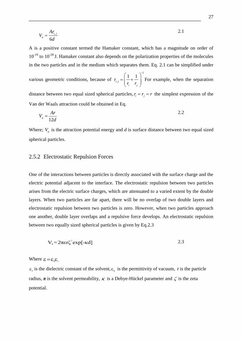
2.5.2 Electrostatic Repulsion Forces
One of the interactions between particles is directly associated with the surface charge and the
electric potential adjacent to the interface. The electrostatic repulsion between two particles
arises from the electric surface charges, which are attenuated to a varied extent by the double
layers. When two particles are far apart, there will be no overlap of two double layers and
electrostatic repulsion between two particles is zero. However, when two particles approach
one another, double layer overlaps and a repulsive force develops. An electrostatic repulsion
between two equally sized spherical particles is given by Eq.2.3
2
RV =2πεrζ exp[-κd] 2.3
Where 0 r
r is the dielectric constant of the solvent, is the permittivity of vacuum, r is the particle
radius, π is the solvent permeability, is a Debye-Hückel parameter and is the zeta
potential.

28
2.5.3 DLVO theory
In 1945, Derjaguin, Landau, Verwey and Overbeek developed a theory to explain the
aggregation of aqueous dispersions quantitatively. This theory is called DLVO theory
(B.D.Derjaguin 1939; L.D.Landau 1941). The theory describes the forces between charged
surfaces interacting through a liquid medium. It combines the effects of the van der Waals
attraction force and the repulsive electrostatic double-layer force. These forces are
sometimes referred to as DLVO forces. The stability of the colloidal suspension is treated in
terms of energy changes by taking whenever particles approach one another. For instance
stabilization can be considered in the case of relation of adding electrolyte into the
suspension. The attractive and repulsive forces are assumed to be additive. And they are also
combined to give the total energy of interaction between particles as a function of separation
distance. DLVO theory suggests that the stability of a particle in solution is dependent upon
its total potential energy function VT. Theoretically, the total potential energy is expressed as
sum as seen below
T A R SV =V +V +V
2.4
Where VS is the potential energy due to the solvent, usually it makes only a marginal
contribution to the total potential energy over the last few nanometers of separation. Much
more important is the balance between attractive potential VA and the repulsive potential VR.
They potentially are much larger and also operate over a much larger distance. The potential
energy due to the solvent is negligible and therefore neglected.
More generally, DLVO theory proposes that the stability of a colloidal system is determined
by the sum of these Van der Waals attractive (VA) and electrical double layer repulsive (VR)
potential that exist between particles as they approach each other due to the Brownian motion
they are undergoing.
T A RV =V +V 2.5
van der Waals attractive potential (VA) promote coagulation while double layer potential (VR)
stabilizes dispersions. Taking into account both equations as 2.2 and 2.3, we can approximate
total energy between the particles. Due to the total energy, when two particles come close to
one another, the explanation of the energy potential can be expressed by using the distance
between the particles. The relationship between the interaction energy potential and the
separation distance of the particles can be explained with the help of stabilization of the
system shown in Figure 2-2. This Figure 2-2 shows the van der Waals attraction potential,
electric repulsion potential, and the combination of the two opposite potentials as a function
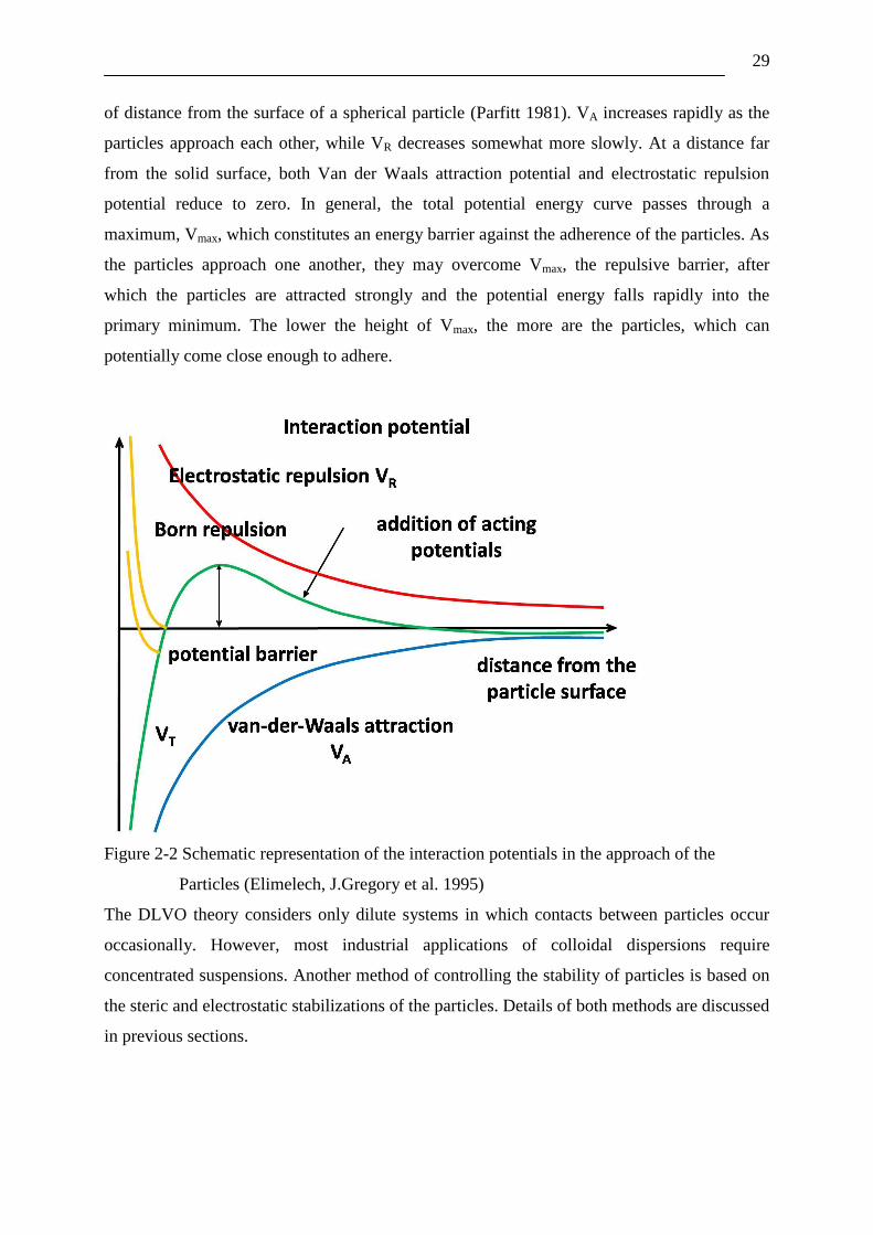
29
of distance from the surface of a spherical particle (Parfitt 1981). VA increases rapidly as the
particles approach each other, while VR decreases somewhat more slowly. At a distance far
from the solid surface, both Van der Waals attraction potential and electrostatic repulsion
potential reduce to zero. In general, the total potential energy curve passes through a
maximum, Vmax, which constitutes an energy barrier against the adherence of the particles. As
the particles approach one another, they may overcome Vmax, the repulsive barrier, after
which the particles are attracted strongly and the potential energy falls rapidly into the
primary minimum. The lower the height of Vmax, the more are the particles, which can
potentially come close enough to adhere.
Figure 2-2 Schematic representation of the interaction potentials in the approach of the
Particles (Elimelech, J.Gregory et al. 1995)
The DLVO theory considers only dilute systems in which contacts between particles occur
occasionally. However, most industrial applications of colloidal dispersions require
concentrated suspensions. Another method of controlling the stability of particles is based on
the steric and electrostatic stabilizations of the particles. Details of both methods are discussed
in previous sections.

30
2.5.4 Steric Interaction
Adsorption is another kinetic mechanism happening during the aggregation process. One of
the important roles of aggregation phenomena is played by adsorbed layers. The steric
interaction comes to the colloidal particulate suspension when there is a large amount of
polymeric concentration. These polymers make the particle surface become or even
overwhelm with the adsorbed layers. As the particles move closer to each other, the layers
come into contact involving the interpretation of the hydrophilic chains. If these chains are
hydrated, these overlapped layers would get some dehydration. And also it increases in both
the free energy and the repulsion between particles.
2.6 Colloidal Stabilization
Stability of colloidal particles means the ability of the particle in suspension stays in the
solution as long as possible without any disturbance in both physical and chemical way.
Stability of dispersion is one of the most important physical properties required for industrial
suspension products such as paints and inks. The dispersion stability governs the ease of
production; storage stability, application properties, and the performance of finished products.
There are two fundamental mechanisms that affect dispersion stability: electrostatic
stabilization and steric stabilization. Types of colloidal stabilization are shown in Figure 2-3.
Each mechanism has its benefits for particulate systems (Napper 1983).
Figure 2-3 Types of colloidal stabilization

31
2.6.1 Steric Stabilization
Steric stabilization, well known as polymeric stabilization, is a method widely used in
stabilization of colloidal dispersions. It is less well understood as compared with electrostatic
stabilization method. It is a simple process requiring just the addition of a suitable polymer.
This involves polymers added to the system adsorbing onto the particle surface and causing
repulsion. Whenever the colloidal suspension has a polymer molecule in the solution, the
particle in the suspension is adsorbed by the polymer on its surface as a layer. The polymer
molecule on the particle surface categorizes into two types- homopolymer and copolymer
(graft copolymer and block copolymer). The resulting polymer layer masks the attractive
force and also provides a repulsive force. This is what we know as “Polymer-induced
stability”. The polymer induced stability is often referred to as steric stability. Steric
stabilization of the colloidal dispersion is achieved by the long chain molecules of colloidal
particles. When they approach to one another due to the Brownian motion, the limited
interpenetration of the polymer chain leads to an effective repulsion stabilizing the suspension
against flocculation.
2.6.2 Electrostatic Stabilization
An electrostatic interaction between charged particles, molecules and ions is the central theme
of colloidal science. This stabilization occurs when there are charges on the surface of the
particle. It is because the surface charge influences the distribution of nearby ions in the polar
medium. It also concerns about a major aspect of the electrostatic stabilization of colloids.
The surface charge occurs whenever the different phases between solids and liquids in the
colloid suspensions are in contact with each other in the polar medium. The stability depends
on the balance of particle interaction, between attraction and repulsion forces. But the
problem is that the configuration of particles inside the fluid is not as simple as anybody could
imagine. Each particle consists of layers, containing ions with different signs. There are also
interactions between ions and particles forming electrical double layers as in Figure 2-4.
Consider a negative particle inside the fluid as an example. The surface potential named as
Nernst potential 0 . The fluid contains ions with different signs and with particles called
counter-ions (here, positive sign) and ion with the same sign called co-ions (here, negative
sign). Because of the electroneutrality principle, counter-ions are attracted toward the particle
surface. A part of these counter-ions called potential determining ions is adsorbed directly on
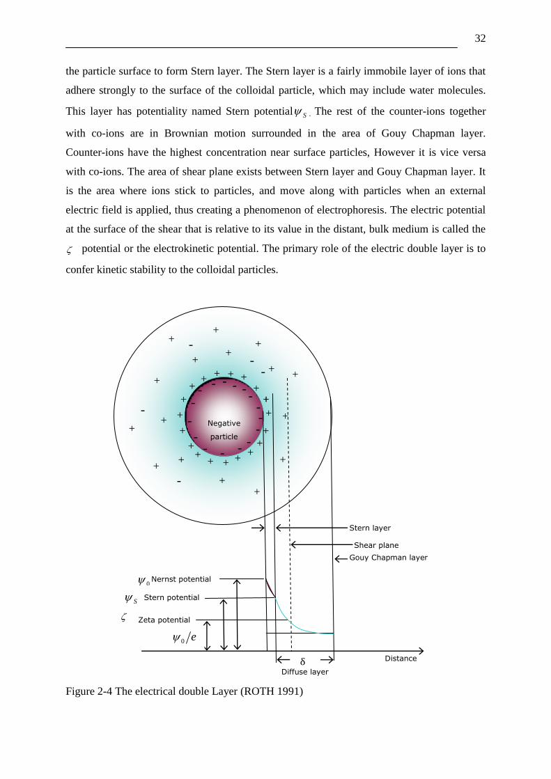
32
the particle surface to form Stern layer. The Stern layer is a fairly immobile layer of ions that
adhere strongly to the surface of the colloidal particle, which may include water molecules.
This layer has potentiality named Stern potential S . The rest of the counter-ions together
with co-ions are in Brownian motion surrounded in the area of Gouy Chapman layer.
Counter-ions have the highest concentration near surface particles, However it is vice versa
with co-ions. The area of shear plane exists between Stern layer and Gouy Chapman layer. It
is the area where ions stick to particles, and move along with particles when an external
electric field is applied, thus creating a phenomenon of electrophoresis. The electric potential
at the surface of the shear that is relative to its value in the distant, bulk medium is called the
potential or the electrokinetic potential. The primary role of the electric double layer is to
confer kinetic stability to the colloidal particles.
Figure 2-4 The electrical double Layer (ROTH 1991)
Negative
particle
- -
- -
-
-
- -
-
-
- -
-
- -
-
+ +
+
+
+ +
+ + + +
+ +
+
+
+ + +
+
+
+
+
+
+
+ +
-
+
+
+
+
+
+
+
+
+
+ +
Stern layer
Shear plane
Stern potential
Zeta potential
Gouy Chapman layer
Nernst potential
Distance
Diffuse layer
-
-
-
-
-
0
φ
0
S
δ
0 e
33
The simplest quantitative treatment to the diffuse part of the double layer of a flat surface is
given by Gouy and Chapman on the following assumptions.
The ions in the diffuse part are point charges distributed according to the Boltzmann
distribution.
The surface is flat and of infinite extent and uniformly charged.
There is only a single electrolyte, which is symmetrical and has charge number.
The solvent influences the double layer only through its dielectric constant, which is
assumed to have the same value throughout the diffuse part.
For the practical calculations here we used, the thickness of the electrochemical double layer
is the Debye length δк the decrease of the potential to 1/e of the surface potential (Elimelech,
J.Gregory et al. 1995)
0
2 2exp
r B
S A i i
k Tdand
e N c z
2.6
where as
S Stern potential 0 Absolute dielectric constant
Potential at distance d r Relative dielectric constant
d Distance from the particle surface Bk Boltzmann constant, 1.38x10
-23 J/K
Debye length = 1 e elementary charge, 1.6x10
-19 C
AN Avogadro constant ic Concentration of ions
T Temperature iz Valence of ions
2.6.3 Zeta Potential
In the colloidal chemistry, zeta potential is usually denoted by using the Greek letter zeta δ,
therefore known as δ-potential. Zeta potential is the potential difference between the
dispersion medium and the stationary layer of fluid attached to the dispersed particle. When
colloidal liquid moves tangential to a charged surface then zeta potential is termed as an
electro-kinetic phenomena(Butt, K Graf et al. 2006). The significance of zeta potential is that
its value can be related to the stability of colloidal dispersion. The zeta potential indicates the
degree of repulsion between adjacent, similarly charged particles in dispersion. Most particles
dispersed in an aqueous system will acquire a surface charge, principally either by ionization
of surface groups, or adsorption of charged species. These surface charges modify the

34
distribution of the surrounding ions, resulting in a layer around the particle that is different to
the bulk solution. Almost all particulate or macroscopic materials in contact with a liquid
acquire an electric charge on their surfaces. Zeta potential is an important and useful
indicator of this charge, which can be used to predict and control the stability of colloidal
suspensions or emulsions (Corporation 1976). The greater the zeta potential, the more likely
the suspension is to be stable because the charged particles repel one another and thus
overcome the natural tendency to agglomerate.
This fundamental aspect is useful to study the synthesis of silver and titania nanoparticles
through the chemical reduction and sol-gel process. The nanoparticles are further modified
with different surfactants by means of steric stabilization. Particles are finally isolated in
powder form and characterized by different techniques. The next chapter describes in detail
all the characterization techniques that were performed for silver and titania nanoparticles.

35
Chapter 3
Characterization methods of Nanoparticles
“The important thing in science is not so much to obtain new facts as to discover new ways of
thinking about them.” – William Bragg Sr.

36
3 Characterization methods of Nanoparticles
article characterization is important to the study and the control of both the processing
and properties of particles. Moreover, as the particles are not of any single size and shape,
information about the average particle size and the distribution of the sizes about the average
is required. The most important characteristics of a particle are its size, shape and density. It
must be recognized that the term „characterization‟ is often used in the literature of material
sciences with a broader meaning. Physical properties determinations are, of course of the
greatest importance in material science and technology.
The parameters generally used to characterize nanoparticles include size, morphology and
surface charge. Particle size and zeta potential were measured using Dynamic Light Scattering
method (DLS). Scanning Electron Microscopy (SEM) and Transmission Electron Microscopy
(TEM) are related techniques that use an electron beam to image a sample. SEM and TEM
were used to observe the topography, morphology, and crystallographic information of the
samples.
3.1 Particle Size Distribution
A particle may be defined as a single entity comprising part of a solid or a liquid
discontinuous phase. Commonly, a suspension of particles in a gas is referred to as aerosol
and particles in suspension in a liquid as sol (hydrosol if the liquid is water). Clearly, when
we are considering the stability of a suspension, particle size becomes important. A number of
methods based on different physical principles exist for measuring particle sizes (PS) and
particle size distribution (PSD). The degree of dispersion also is important and is affected by
sample distribution. The distribution in the size of the particles is dependent at any time on
the rate of formation of the particles. Generally, at steady state, the rate of agglomeration and
the rate of disintegration are the same. That means, the steady state is very important in
determining the particle size distribution.
When particles divide into a number of individuals within a size fraction or an interval i , it is
called as number distribution. The preferred method of presenting the size data is to divide the
individual count by the total number of counts, to obtain the fractional count in each size
class, and then to divide this fraction by the interval width. The resulting representation has an
important property. This property states that the area under each rectangle represents the
fraction of particles in the interval.
P
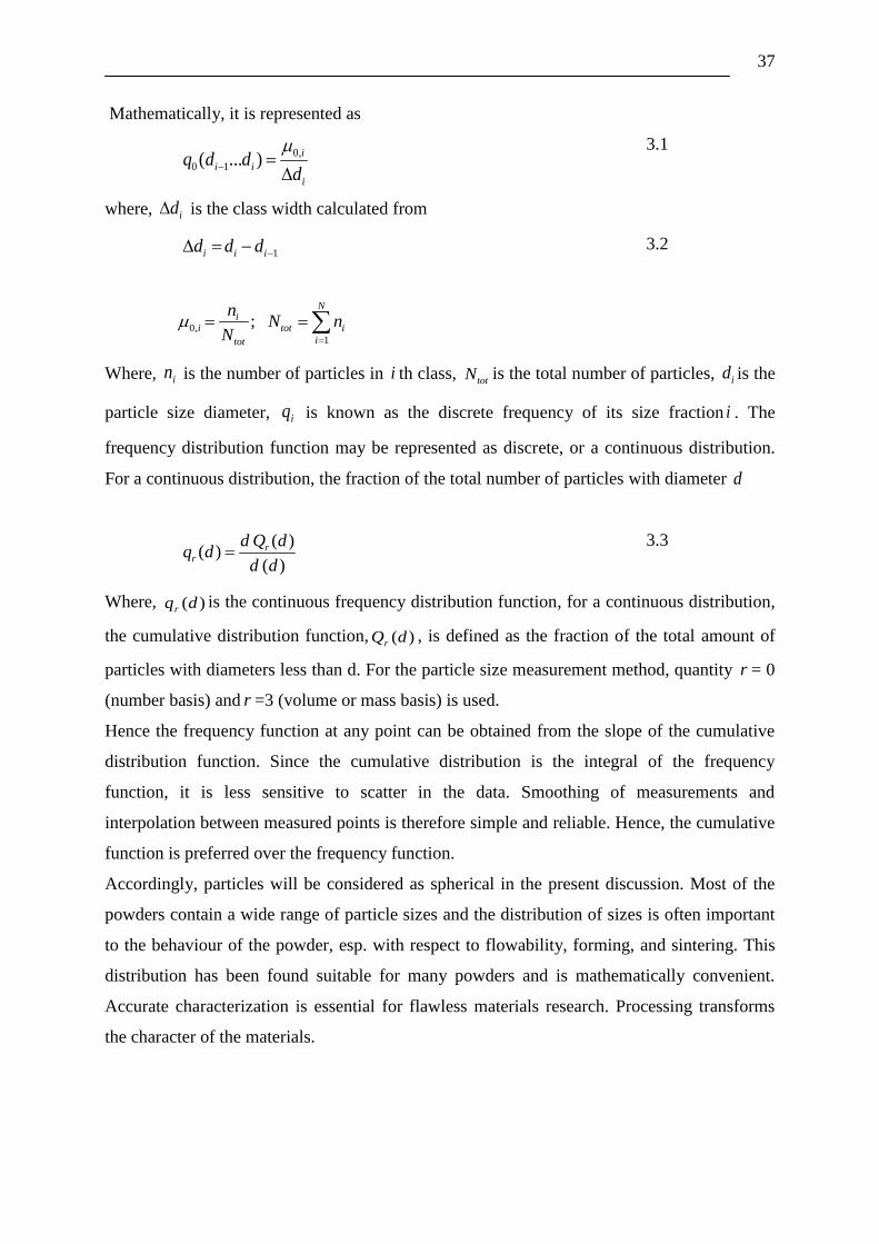
37
Mathematically, it is represented as
0,
0 1( ... )i
i i
i
q d dd
3.1
where, id is the class width calculated from
1i i id d d 3.2
0,
1
;N
ii tot i
itot
nN n
N
Where, in is the number of particles in i th class, totN is the total number of particles, id is the
particle size diameter, iq is known as the discrete frequency of its size fraction i . The
frequency distribution function may be represented as discrete, or a continuous distribution.
For a continuous distribution, the fraction of the total number of particles with diameter d
( )
( )( )
rr
d Q dq d
d d
3.3
Where, )(dqris the continuous frequency distribution function, for a continuous distribution,
the cumulative distribution function, )(dQr, is defined as the fraction of the total amount of
particles with diameters less than d. For the particle size measurement method, quantity r = 0
(number basis) and r =3 (volume or mass basis) is used.
Hence the frequency function at any point can be obtained from the slope of the cumulative
distribution function. Since the cumulative distribution is the integral of the frequency
function, it is less sensitive to scatter in the data. Smoothing of measurements and
interpolation between measured points is therefore simple and reliable. Hence, the cumulative
function is preferred over the frequency function.
Accordingly, particles will be considered as spherical in the present discussion. Most of the
powders contain a wide range of particle sizes and the distribution of sizes is often important
to the behaviour of the powder, esp. with respect to flowability, forming, and sintering. This
distribution has been found suitable for many powders and is mathematically convenient.
Accurate characterization is essential for flawless materials research. Processing transforms
the character of the materials.
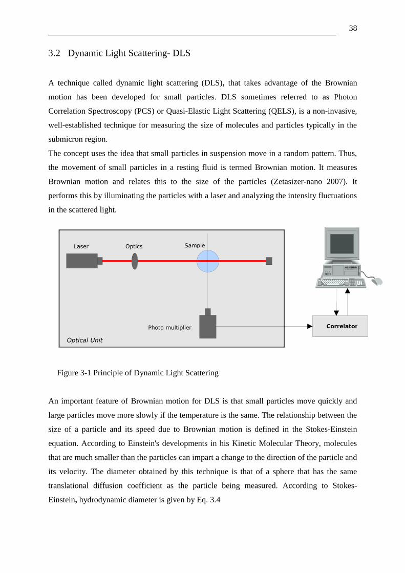
38
3.2 Dynamic Light Scattering- DLS
A technique called dynamic light scattering (DLS), that takes advantage of the Brownian
motion has been developed for small particles. DLS sometimes referred to as Photon
Correlation Spectroscopy (PCS) or Quasi-Elastic Light Scattering (QELS), is a non-invasive,
well-established technique for measuring the size of molecules and particles typically in the
submicron region.
The concept uses the idea that small particles in suspension move in a random pattern. Thus,
the movement of small particles in a resting fluid is termed Brownian motion. It measures
Brownian motion and relates this to the size of the particles (Zetasizer-nano 2007). It
performs this by illuminating the particles with a laser and analyzing the intensity fluctuations
in the scattered light.
Figure 3-1 Principle of Dynamic Light Scattering
An important feature of Brownian motion for DLS is that small particles move quickly and
large particles move more slowly if the temperature is the same. The relationship between the
size of a particle and its speed due to Brownian motion is defined in the Stokes-Einstein
equation. According to Einstein's developments in his Kinetic Molecular Theory, molecules
that are much smaller than the particles can impart a change to the direction of the particle and
its velocity. The diameter obtained by this technique is that of a sphere that has the same
translational diffusion coefficient as the particle being measured. According to Stokes-
Einstein, hydrodynamic diameter is given by Eq. 3.4
Laser Optics Sample
Photo multiplier Correlator
Optical Unit
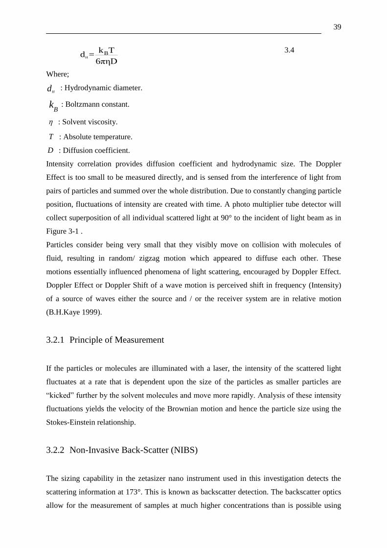
39
H
Bk Td =
6πηD
3.4
Where;
Hd : Hydrodynamic diameter.
B
k : Boltzmann constant.
: Solvent viscosity.
T : Absolute temperature.
D : Diffusion coefficient.
Intensity correlation provides diffusion coefficient and hydrodynamic size. The Doppler
Effect is too small to be measured directly, and is sensed from the interference of light from
pairs of particles and summed over the whole distribution. Due to constantly changing particle
position, fluctuations of intensity are created with time. A photo multiplier tube detector will
collect superposition of all individual scattered light at 90° to the incident of light beam as in
Figure 3-1 .
Particles consider being very small that they visibly move on collision with molecules of
fluid, resulting in random/ zigzag motion which appeared to diffuse each other. These
motions essentially influenced phenomena of light scattering, encouraged by Doppler Effect.
Doppler Effect or Doppler Shift of a wave motion is perceived shift in frequency (Intensity)
of a source of waves either the source and / or the receiver system are in relative motion
(B.H.Kaye 1999).
3.2.1 Principle of Measurement
If the particles or molecules are illuminated with a laser, the intensity of the scattered light
fluctuates at a rate that is dependent upon the size of the particles as smaller particles are
“kicked” further by the solvent molecules and move more rapidly. Analysis of these intensity
fluctuations yields the velocity of the Brownian motion and hence the particle size using the
Stokes-Einstein relationship.
3.2.2 Non-Invasive Back-Scatter (NIBS)
The sizing capability in the zetasizer nano instrument used in this investigation detects the
scattering information at 173°. This is known as backscatter detection. The backscatter optics
allow for the measurement of samples at much higher concentrations than is possible using
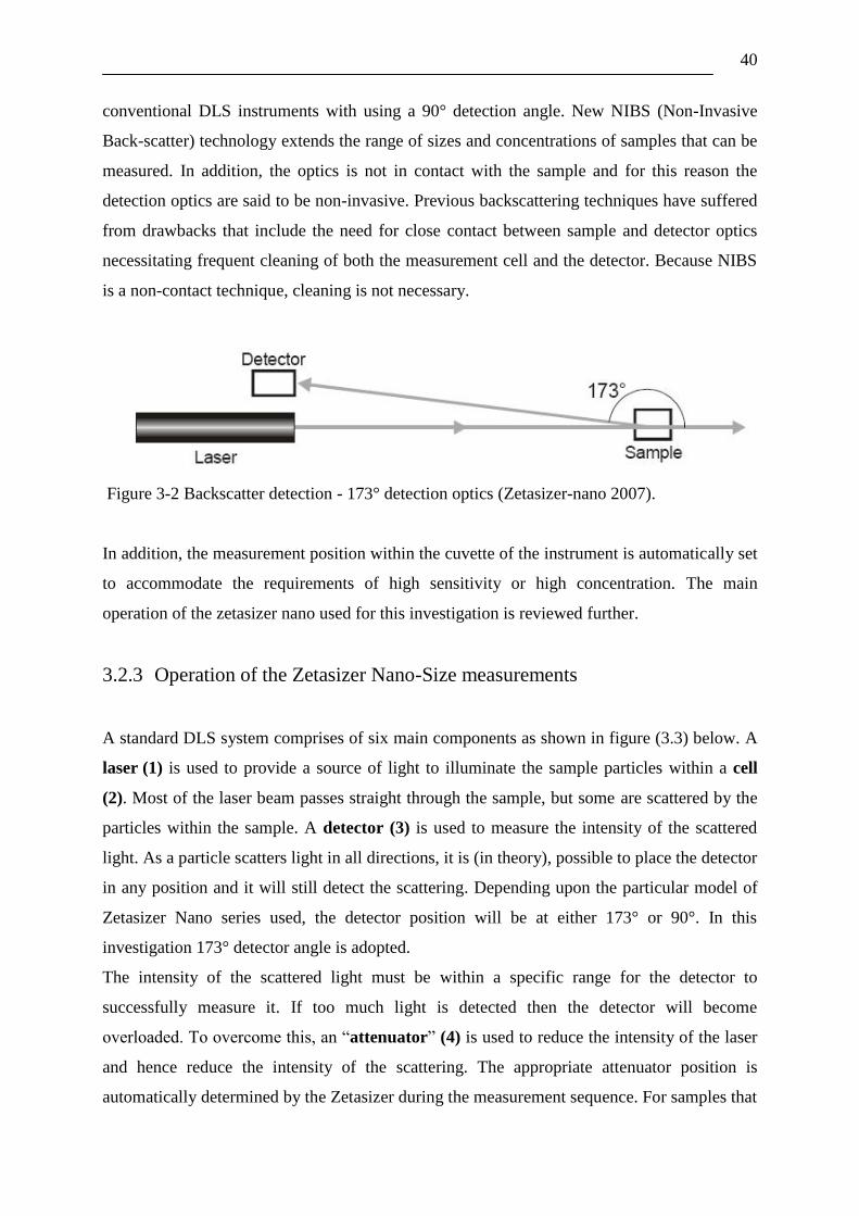
40
conventional DLS instruments with using a 90° detection angle. New NIBS (Non-Invasive
Back-scatter) technology extends the range of sizes and concentrations of samples that can be
measured. In addition, the optics is not in contact with the sample and for this reason the
detection optics are said to be non-invasive. Previous backscattering techniques have suffered
from drawbacks that include the need for close contact between sample and detector optics
necessitating frequent cleaning of both the measurement cell and the detector. Because NIBS
is a non-contact technique, cleaning is not necessary.
Figure 3-2 Backscatter detection - 173° detection optics (Zetasizer-nano 2007).
In addition, the measurement position within the cuvette of the instrument is automatically set
to accommodate the requirements of high sensitivity or high concentration. The main
operation of the zetasizer nano used for this investigation is reviewed further.
3.2.3 Operation of the Zetasizer Nano-Size measurements
A standard DLS system comprises of six main components as shown in figure (3.3) below. A
laser (1) is used to provide a source of light to illuminate the sample particles within a cell
(2). Most of the laser beam passes straight through the sample, but some are scattered by the
particles within the sample. A detector (3) is used to measure the intensity of the scattered
light. As a particle scatters light in all directions, it is (in theory), possible to place the detector
in any position and it will still detect the scattering. Depending upon the particular model of
Zetasizer Nano series used, the detector position will be at either 173° or 90°. In this
investigation 173° detector angle is adopted.
The intensity of the scattered light must be within a specific range for the detector to
successfully measure it. If too much light is detected then the detector will become
overloaded. To overcome this, an “attenuator” (4) is used to reduce the intensity of the laser
and hence reduce the intensity of the scattering. The appropriate attenuator position is
automatically determined by the Zetasizer during the measurement sequence. For samples that

41
do not scatter much light, such as very small particles or samples of low concentration, the
amount of scattered light must be increased. In such circumstance, the attenuator will allow
more laser light to pass through the sample. The amount of scattered light must be decreased
for samples that scatter more light, such as large particles or samples of higher concentration.
Figure 3-3 Schematic diagram of a standard DLS system (Zetasizer-nano 2007)
This is accomplished by using the attenuator to reduce the amount of laser light that passes
through to the sample. The scattering intensity signal for the detector is passed to a digital
signal processing board known as a correlator (5). The correlator compares the scattering
intensity at successive time intervals to obtain the rate at which the intensity is changing. This
correlator information is finally passed to a computer (6), where the professional Zetasizer
software will analyze the data and derive size information (Zetasizer-nano 2007).
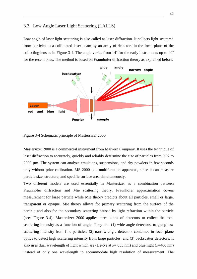
42
3.3 Low Angle Laser Light Scattering (LALLS)
Low angle of laser light scattering is also called as laser diffraction. It collects light scattered
from particles in a collimated laser beam by an array of detectors in the focal plane of the
collecting lens as in Figure 3-4. The angle varies from 14o for the early instruments up to 40
o
for the recent ones. The method is based on Fraunhofer diffraction theory as explained before.
Figure 3-4 Schematic principle of Mastersizer 2000
Mastersizer 2000 is a commercial instrument from Malvern Company. It uses the technique of
laser diffraction to accurately, quickly and reliably determine the size of particles from 0.02 to
2000 µm. The system can analyze emulsions, suspensions, and dry powders in few seconds
only without prior calibration. MS 2000 is a multifunction apparatus, since it can measure
particle size, structure, and specific surface area simultaneously.
Two different models are used essentially in Mastersizer as a combination between
Fraunhofer diffraction and Mie scattering theory. Fraunhofer approximation covers
measurement for large particle while Mie theory predicts about all particles, small or large,
transparent or opaque. Mie theory allows for primary scattering from the surface of the
particle and also for the secondary scattering caused by light refraction within the particle
(sees Figure 3-4). Mastersizer 2000 applies three kinds of detectors to collect the total
scattering intensity as a function of angle. They are: (1) wide angle detectors, to grasp low
scattering intensity from fine particles; (2) narrow angle detectors contained in focal plane
optics to detect high scattering intensity from large particles; and (3) backscatter detectors. It
also uses dual wavelength of light which are (He-Ne at λ= 633 nm) and blue light (λ=466 nm)
instead of only one wavelength to accommodate high resolution of measurement. The
Laser
backscatter
detector
wide angle
detector narrow angle
detector
Fourier
lens
sample
chamber
red and blue light
sources
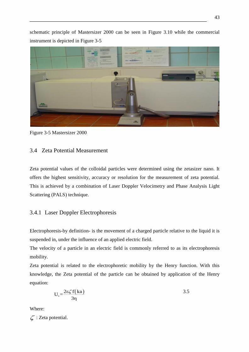
43
schematic principle of Mastersizer 2000 can be seen in Figure 3.10 while the commercial
instrument is depicted in Figure 3-5
Figure 3-5 Mastersizer 2000
3.4 Zeta Potential Measurement
Zeta potential values of the colloidal particles were determined using the zetasizer nano. It
offers the highest sensitivity, accuracy or resolution for the measurement of zeta potential.
This is achieved by a combination of Laser Doppler Velocimetry and Phase Analysis Light
Scattering (PALS) technique.
3.4.1 Laser Doppler Electrophoresis
Electrophoresis-by definition- is the movement of a charged particle relative to the liquid it is
suspended in, under the influence of an applied electric field.
The velocity of a particle in an electric field is commonly referred to as its electrophoresis
mobility.
Zeta potential is related to the electrophoretic mobility by the Henry function. With this
knowledge, the Zeta potential of the particle can be obtained by application of the Henry
equation:
E
2ε f kaU =
3η
3.5
Where:
: Zeta potential.

44
EU : Electrophoretic mobility.
: Dielectric constant.
: Viscosity.
( )f Ka : Henry‟s function.
Two values are generally used as approximations for the f (Ka) determination, either 1.5 or
1.0. Electrophoretic determinations of Zeta potential are most commonly made in aqueous
media and moderate electrolyte concentration. f (Ka) in this case is 1.5, and is referred to as
the Smoluchowski approximation. Therefore calculation of Zeta potential from the mobility is
simple for systems that fit the Smoluchowski model. The Smoluchowski approximation is
used for the folded capillary cell and the universal dip cell when used with aqueous samples.
For small particles in low dielectric constant media, f (Ka) becomes 1.0 and permits an
equally simple calculation. This is referred to as the Hückel approximation. Non-aqueous
measurements generally use this principle (Zetasizer-nano 2007).
3.4.2 Measuring Electrophoretical Mobility
Electrophoresis mobility is measured directly from experiments and further converted to Zeta
potential using theoretical considerations. The fundamental nature of a classical
electrophoresis system is a cell with electrodes at either end to which a potential is applied.
Figure 3.5 vividly portrays it. Particles move towards the electrode of opposite charge, their
velocity is measured and expressed in unit field strength as their mobility. The technique used
to measure this velocity is Laser Doppler Velocimetry which is described in Figure 3-6.
Figure 3-6 Measurement of Electrophoretic Mobility (Zetasizer-nano 2007)

45
3.4.3 Laser Doppler Velocimetry
Laser Doppler Velocimetry (LDV) is a well recognized technique in engineering for the study
of fluid flow in a wide variety of situations. The actual velocity of tiny particles within the
fluid streams moving at the velocity of the fluid are measured. LDV is therefore devised to
measure the velocity of particles moving through a fluid in an electrophoresis experiment.
Figure 3-7 is a typical illustration of LDV system. The receiving optics is focused so as to
relay the scattering of particles in the cell. The light scattered at an angle of 17° is combined
with the reference beam. This produces a fluctuating intensity signal where the rate of
fluctuation is proportional to the speed of the particles. A digital signal processor is used to
extract the characteristic frequencies in the scattered light.
Figure 3-7 Laser Doppler Velocimetry (Zetasizer-nano 2007)
3.4.4 Operation of the Zetasizer Nano- Zeta potential measurements
Similar to the typical DLS system described previously in the size measurement, zeta
potential measurement system consists of six main components (Figure 3-8). A laser (1) is
used to provide a source of light to illuminate the particles within the sample. For Zeta
potential measurements this source of light is split to provide an incident and reference beam.
The reference beam is also „modulated‟ to provide the necessary, Doppler Effect. The laser
beam passes through the centre of the sample cell (2), and the scattering at an angle of 17° is
detected.

46
A detector (3) sends this information to a digital signal processor (4). This information is
then passed to a computer (5), where the Zetasizer Nano software generates a frequency
spectrum from which the electrophoretic mobility and hence the Zeta potential information is
calculated.
The intensity of the scattered light within the cell must be within a specific range for the
detector to successfully measure it. If too much light is detected then the detector will be
overloaded. To overcome this, an attenuator (6) is used to reduce the intensity of the laser
and hence reduce the intensity of the scattering.
The amount of scattered light must be increased for samples that do not scatter much light,
For samples that scatter more light, such as large particles or samples of higher concentration,
the amount of scattered light must be reduced. The attenuator will automatically reduce the
amount of light that passes through to the sample.
Figure 3-8 Operation of the Zeta potential measurements (Zetasizer-nano 2007)
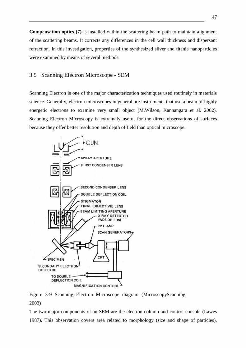
47
Compensation optics (7) is installed within the scattering beam path to maintain alignment
of the scattering beams. It corrects any differences in the cell wall thickness and dispersant
refraction. In this investigation, properties of the synthesized silver and titania nanoparticles
were examined by means of several methods.
3.5 Scanning Electron Microscope - SEM
Scanning Electron is one of the major characterization techniques used routinely in materials
science. Generally, electron microscopes in general are instruments that use a beam of highly
energetic electrons to examine very small object (M.Wilson, Kannangara et al. 2002).
Scanning Electron Microscopy is extremely useful for the direct observations of surfaces
because they offer better resolution and depth of field than optical microscope.
Figure 3-9 Scanning Electron Microscope diagram (MicroscopyScanning
2003)
The two major components of an SEM are the electron column and control console (Lawes
1987). This observation covers area related to morphology (size and shape of particles),
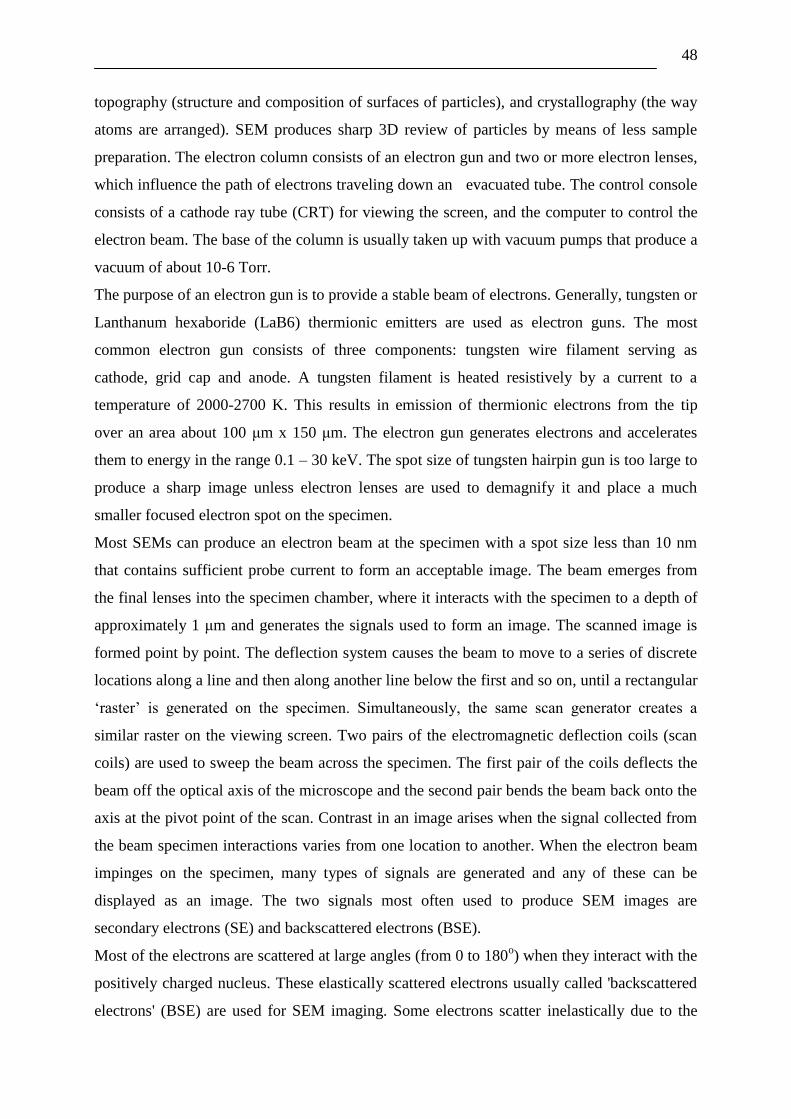
48
topography (structure and composition of surfaces of particles), and crystallography (the way
atoms are arranged). SEM produces sharp 3D review of particles by means of less sample
preparation. The electron column consists of an electron gun and two or more electron lenses,
which influence the path of electrons traveling down an evacuated tube. The control console
consists of a cathode ray tube (CRT) for viewing the screen, and the computer to control the
electron beam. The base of the column is usually taken up with vacuum pumps that produce a
vacuum of about 10-6 Torr.
The purpose of an electron gun is to provide a stable beam of electrons. Generally, tungsten or
Lanthanum hexaboride (LaB6) thermionic emitters are used as electron guns. The most
common electron gun consists of three components: tungsten wire filament serving as
cathode, grid cap and anode. A tungsten filament is heated resistively by a current to a
temperature of 2000-2700 K. This results in emission of thermionic electrons from the tip
over an area about 100 μm x 150 μm. The electron gun generates electrons and accelerates
them to energy in the range 0.1 – 30 keV. The spot size of tungsten hairpin gun is too large to
produce a sharp image unless electron lenses are used to demagnify it and place a much
smaller focused electron spot on the specimen.
Most SEMs can produce an electron beam at the specimen with a spot size less than 10 nm
that contains sufficient probe current to form an acceptable image. The beam emerges from
the final lenses into the specimen chamber, where it interacts with the specimen to a depth of
approximately 1 μm and generates the signals used to form an image. The scanned image is
formed point by point. The deflection system causes the beam to move to a series of discrete
locations along a line and then along another line below the first and so on, until a rectangular
„raster‟ is generated on the specimen. Simultaneously, the same scan generator creates a
similar raster on the viewing screen. Two pairs of the electromagnetic deflection coils (scan
coils) are used to sweep the beam across the specimen. The first pair of the coils deflects the
beam off the optical axis of the microscope and the second pair bends the beam back onto the
axis at the pivot point of the scan. Contrast in an image arises when the signal collected from
the beam specimen interactions varies from one location to another. When the electron beam
impinges on the specimen, many types of signals are generated and any of these can be
displayed as an image. The two signals most often used to produce SEM images are
secondary electrons (SE) and backscattered electrons (BSE).
Most of the electrons are scattered at large angles (from 0 to 180o) when they interact with the
positively charged nucleus. These elastically scattered electrons usually called 'backscattered
electrons' (BSE) are used for SEM imaging. Some electrons scatter inelastically due to the
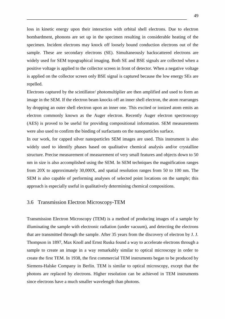
49
loss in kinetic energy upon their interaction with orbital shell electrons. Due to electron
bombardment, phonons are set up in the specimen resulting in considerable heating of the
specimen. Incident electrons may knock off loosely bound conduction electrons out of the
sample. These are secondary electrons (SE). Simultaneously backscattered electrons are
widely used for SEM topographical imaging. Both SE and BSE signals are collected when a
positive voltage is applied to the collector screen in front of detector. When a negative voltage
is applied on the collector screen only BSE signal is captured because the low energy SEs are
repelled.
Electrons captured by the scintillator/ photomultiplier are then amplified and used to form an
image in the SEM. If the electron beam knocks off an inner shell electron, the atom rearranges
by dropping an outer shell electron upon an inner one. This excited or ionized atom emits an
electron commonly known as the Auger electron. Recently Auger electron spectroscopy
(AES) is proved to be useful for providing compositional information. SEM measurements
were also used to confirm the binding of surfactants on the nanoparticles surface.
In our work, for capped silver nanoparticles SEM images are used. This instrument is also
widely used to identify phases based on qualitative chemical analysis and/or crystalline
structure. Precise measurement of measurement of very small features and objects down to 50
nm in size is also accomplished using the SEM. In SEM techniques the magnification ranges
from 20X to approximately 30,000X, and spatial resolution ranges from 50 to 100 nm. The
SEM is also capable of performing analyses of selected point locations on the sample; this
approach is especially useful in qualitatively determining chemical compositions.
3.6 Transmission Electron Microscopy-TEM
Transmission Electron Microscopy (TEM) is a method of producing images of a sample by
illuminating the sample with electronic radiation (under vacuum), and detecting the electrons
that are transmitted through the sample. After 35 years from the discovery of electron by J. J.
Thompson in 1897, Max Knoll and Ernst Ruska found a way to accelerate electrons through a
sample to create an image in a way remarkably similar to optical microscopy in order to
create the first TEM. In 1938, the first commercial TEM instruments began to be produced by
Siemens-Halske Company in Berlin. TEM is similar to optical microscopy, except that the
photons are replaced by electrons. Higher resolution can be achieved in TEM instruments
since electrons have a much smaller wavelength than photons.

50
The electron gun usually consists of a tungsten wire filament, which is bent into a hairpin
("V") shape and surrounded by a shield with a circular aperture (1-3 mm diameter) centered
just below the filament tip as shown in Figure 3-10 . Electrons in the gun are accelerated
across a potential difference of the order of 100,000 volts between the cathode (at high
negative potential) and anode (at ground potential). The function of the condenser lens is to
focus the electron beam emerging from the electron gun onto the specimen to permit optimal
illuminating conditions for visualizing and recording the image. The optical enlarging system
of an electron microscope consists of an objective lens followed by one or more projector
lenses. The objective lens determines resolution and contrast in the image, and all
subsequent lenses bring the final image to a convenient magnification for observation and
recording. The objective lens is the most critical lens since it determines the resolving power
of the instrument and performs the first stage of imaging. The specimen image generated by
the objective lens is subsequently magnified in one or two more magnification stages by the
intermediate and projector lens, and then projected onto a fluorescent screen or photographic
plate. In this work, measurements were performed on a CM200 of the firm Philips/FEI
instrument operated at an accelerating voltage of 200 kV.

51
Figure 3-10 Transmission Electron Microscope (Wikipedia 2009)
TEM is the ultimate in situ high resolution electron microscope to study dynamic behavior of
chemical reactions under the influence of variable temperatures and gas pressures at the
atomic level. In our work, for double reduction of silver nanoparticles TEM images are used.
A TEM image describes the morphology, structure, composition and bonding of
nanomaterials down to the atomic level. In TEM techniques, the Point of resolution is up to
≥0.12 nm, and particle size is down to 5 nm.
52
Chapter 4
Experimental Set up and
Synthesis of Materials
“In science one tries to tell people, in such a way as to be understood by everyone, something
that no one ever knew before. But in poetry, it's the exact opposite.”
-Paul Dirac

53
4 Experimental Set up and Synthesis of Materials
This chapter elucidates the synthesis of silver nanoparticles by using capping agent along with
reducing agent. The second part deals with synthesis and surface stabilization of sol-gel TiO2
nanoparticles by means of sol-gel process with different surfactants.
This chapter contains experimental procedures, scientific data of the materials, capping
agents, surfactants, and reducing agents. A list of chemicals and solvents used is also included
in this chapter
4.1 Experimental Set up
This section demonstrates and explains the experimental methodology and procedure for
producing oxide and noble nanoparticles under the chemical reduction and sol-gel
precipitation process.
4.1.1 Types and Characteristics of Stirrer
he focus will now be on the apparatuses commonly used for producing and measuring
particle sizes, structures, and shapes. Nanoparticles are usually generated inside stirred
tank reactor or vessel cylindrical in form with a vertical axis. A standardized design of a
vessel is similar to Figure 4-1, however detail design depends on the requirement of different
situations. Impeller, heater or cooler in form of jacket or thermostat, thermometer device,
baffles, speed control and drain valve are the accessories provided. A motor drives an
impeller, which is mounted on an overhung shaft. The impeller causes the liquid to circulate
through the vessel and eventually return to the impeller. While all of this happens, the
homogeneous system in the vessel is maintained.
The three main types of stirrers for low to moderate viscosity liquids are propellers, turbines,
and high efficiency impellers. The standard three-blade marine propeller, which is a
frequently used impeller, belongs to the category of propeller impellers. While the six-blade
turbines belong to the turbines impellers as in Figure 4-2. Highly viscous liquids are treated
with helical impellers and anchor agitator. When solid particles are present in the system, they
are often responsible for the swirling or circulatory pattern. And when this pattern occurs, the
particles are thrown the outside by the centrifugal force, and moved downward to the center
T
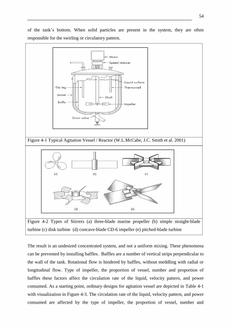
54
of the tank‟s bottom. When solid particles are present in the system, they are often
responsible for the swirling or circulatory pattern.
Figure 4-1 Typical Agitation Vessel / Reactor (W.L.McCabe, J.C. Smith et al. 2001)
Figure 4-2 Types of Stirrers (a) three-blade marine propeller (b) simple straight-blade
turbine (c) disk turbine (d) concave-blade CD-6 impeller (e) pitched-blade turbine
The result is an undesired concentrated system, and not a uniform mixing. These phenomena
can be prevented by installing baffles. Baffles are a number of vertical strips perpendicular to
the wall of the tank. Rotational flow is hindered by baffles, without meddling with radial or
longitudinal flow. Type of impeller, the proportion of vessel, number and proportion of
baffles these factors affect the circulation rate of the liquid, velocity pattern, and power
consumed. As a starting point, ordinary designs for agitation vessel are depicted in Table 4-1
with visualization in Figure 4-3. The circulation rate of the liquid, velocity pattern, and power
consumed are affected by the type of impeller, the proportion of vessel, number and

55
proportion of baffles (W.L.McCabe, J.C. Smith et al. 2001). Following are the quantities
required: Number of baffles used is usually 4, Number of impeller blades ranges from 4 to 16
but generally 6 or 8. Depth of the liquid should be equal to or somewhat greater than the
diameter of the tank. Figure 4-3 shows schematic diagram of stirred tank reactor. If greater
depth is desired, then mount two or more impellers on the same shaft. Two separate
circulation patterns are formed when flat turbines give a good radial flow in the plane of
impeller, while the flow divides at the wall. One portion flows downward along the wall and
back to the center of the impeller from below. The other portion flows upward toward the
surface, and back to the impeller from above. Figure 4-4 depicts the pattern under utilization
of turbine impeller and baffles.
Table 4-1 Ordinary design of vessel/ Reactor
Parameters Design Symbols
3
1
D
D
t
a 3
1
D
E
t
Da = diameter of impeller
Dt = diameter of vessel
H = height of liquid
J = baffles width
E = distance of impeller
from bottom of vessel
W = impeller width
L = impeller blade
1D
H
t
5
1
D
W
a
12
1
D
J
t
4
1
D
L
a
Figure 4-3 Schematic of the stirred tank
reactor (J.H.Rushton, Costich et al. 1950)
Figure 4-4 Draft tube : Turbine Impeller
(Bissell, H.C.Hesse et al. 1947)
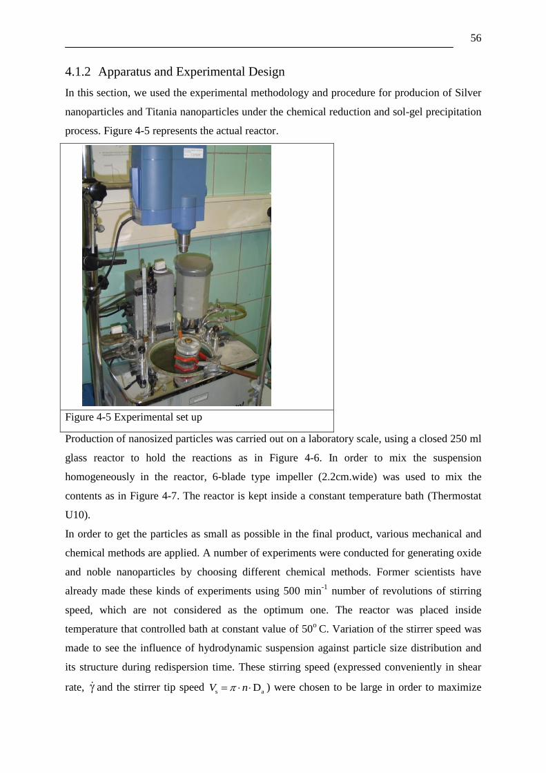
56
4.1.2 Apparatus and Experimental Design
In this section, we used the experimental methodology and procedure for producion of Silver
nanoparticles and Titania nanoparticles under the chemical reduction and sol-gel precipitation
process. Figure 4-5 represents the actual reactor.
Figure 4-5 Experimental set up
Production of nanosized particles was carried out on a laboratory scale, using a closed 250 ml
glass reactor to hold the reactions as in Figure 4-6. In order to mix the suspension
homogeneously in the reactor, 6-blade type impeller (2.2cm.wide) was used to mix the
contents as in Figure 4-7. The reactor is kept inside a constant temperature bath (Thermostat
U10).
In order to get the particles as small as possible in the final product, various mechanical and
chemical methods are applied. A number of experiments were conducted for generating oxide
and noble nanoparticles by choosing different chemical methods. Former scientists have
already made these kinds of experiments using 500 min-1
number of revolutions of stirring
speed, which are not considered as the optimum one. The reactor was placed inside
temperature that controlled bath at constant value of 50o
C. Variation of the stirrer speed was
made to see the influence of hydrodynamic suspension against particle size distribution and
its structure during redispersion time. These stirring speed (expressed conveniently in shear
rate, and the stirrer tip speed s aDV n ) were chosen to be large in order to maximize

57
redispersion of agglomerate and to keep particles away from sedimentation as shown in Table
4-2. The shear rate and Reynolds number calculation are shown in Appendix A.
Figure 4-6 250 ml closed glass reactor
Table 4-2 Variation used in experiments (Kinematics Viscosity = 6.10-7
m2/s)
Number of
revolutions n
in min-1
Stirrer tip speed
sV in m/s
Turbulent energy
dissipation rate
in m2/s
3
Shear rates
in s-1
Reynold
numbers Re
500 0.58 0.069 370 6719
750 0.86 0.233 623 10083
1000 1.15 0.553 960 13447
1250 1.44 1.080 1342 16802
4.2 Silver nanoparticles synthesis
Noble nanoparticles have been extensively investigated because of their unique electronic and
optical properties that are different from bulk materials. In this section, synthesis of silver
nanoparticles is done using bottom-up approach. In comparison with a top-down approach,
bottom- up approach gives the advantage of producing stable silver nanoparticles, by the
formation of defined crystalline nanoparticles structures. Normally a dilute solution of metal
salt, surfactant and reducing reagent leads to the formation of clear golden-yellow colloidal
solution by a bottom-up approach.
Figure 4-7 6-blade an impeller
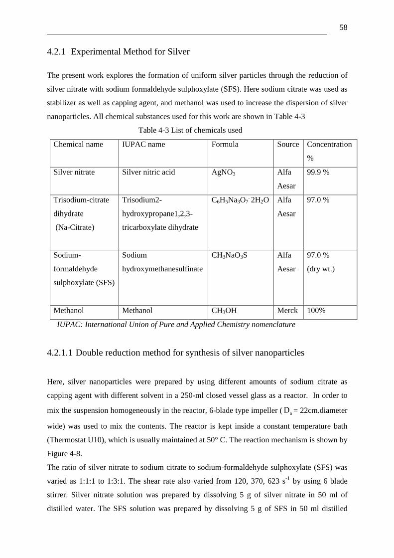
58
4.2.1 Experimental Method for Silver
The present work explores the formation of uniform silver particles through the reduction of
silver nitrate with sodium formaldehyde sulphoxylate (SFS). Here sodium citrate was used as
stabilizer as well as capping agent, and methanol was used to increase the dispersion of silver
nanoparticles. All chemical substances used for this work are shown in Table 4-3
Table 4-3 List of chemicals used
Chemical name IUPAC name Formula Source Concentration
%
Silver nitrate
Silver nitric acid AgNO3 Alfa
Aesar
99.9 %
Trisodium-citrate
dihydrate
(Na-Citrate)
Trisodium2-
hydroxypropane1,2,3-
tricarboxylate dihydrate
C6H5Na3O7. 2H2O Alfa
Aesar
97.0 %
Sodium-
formaldehyde
sulphoxylate (SFS)
Sodium
hydroxymethanesulfinate
CH3NaO3S Alfa
Aesar
97.0 %
(dry wt.)
Methanol Methanol CH3OH Merck 100%
IUPAC: International Union of Pure and Applied Chemistry nomenclature
4.2.1.1 Double reduction method for synthesis of silver nanoparticles
Here, silver nanoparticles were prepared by using different amounts of sodium citrate as
capping agent with different solvent in a 250-ml closed vessel glass as a reactor. In order to
mix the suspension homogeneously in the reactor, 6-blade type impeller ( aD = 22cm.diameter
wide) was used to mix the contents. The reactor is kept inside a constant temperature bath
(Thermostat U10), which is usually maintained at 50° C. The reaction mechanism is shown by
Figure 4-8.
The ratio of silver nitrate to sodium citrate to sodium-formaldehyde sulphoxylate (SFS) was
varied as 1:1:1 to 1:3:1. The shear rate also varied from 120, 370, 623 s-1
by using 6 blade
stirrer. Silver nitrate solution was prepared by dissolving 5 g of silver nitrate in 50 ml of
distilled water. The SFS solution was prepared by dissolving 5 g of SFS in 50 ml distilled
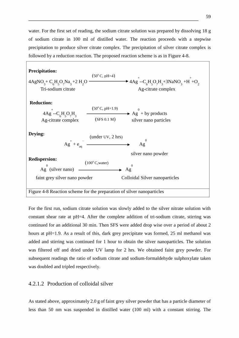
59
water. For the first set of reading, the sodium citrate solution was prepared by dissolving 18 g
of sodium citrate in 100 ml of distilled water. The reaction proceeds with a stepwise
precipitation to produce silver citrate complex. The precipitation of silver citrate complex is
followed by a reduction reaction. The proposed reaction scheme is as in Figure 4-8.
Precipitation:
4AgNO3+ C
6H
5O
7Na
3 +2 H
2O 4Ag
+
--C6H
5O
7H
3+3NaNO
3 +H
+
+O2
Tri-sodium citrate Ag-citrate complex
Reduction:
4Ag+
--C6H
5O
7H
3 Ag
0
+ by products
Ag-citrate complex silver nano particles
Drying:
Ag+ + e
aq
− Ag
0
silver nano powder Redispersion:
Ag0
(silver nano)
Ag
0
faint grey silver nano powder Colloidal Silver nanoparticles
Figure 4-8 Reaction scheme for the preparation of silver nanoparticles
For the first run, sodium citrate solution was slowly added to the silver nitrate solution with
constant shear rate at pH=4. After the complete addition of tri-sodium citrate, stirring was
continued for an additional 30 min. Then SFS were added drop wise over a period of about 2
hours at pH=1.9. As a result of this, dark grey precipitate was formed, 25 ml methanol was
added and stirring was continued for 1 hour to obtain the silver nanoparticles. The solution
was filtered off and dried under UV lamp for 2 hrs. We obtained faint grey powder. For
subsequent readings the ratio of sodium citrate and sodium-formaldehyde sulphoxylate taken
was doubled and tripled respectively.
4.2.1.2 Production of colloidal silver
As stated above, approximately 2.0 g of faint grey silver powder that has a particle diameter of
less than 50 nm was suspended in distilled water (100 ml) with a constant stirring. The
(50o C, pH=4)
(50o C, pH=1.9)
(SFS 0.1 M)
(100o C,water)
(under UV, 2 hrs)

60
suspension was heated to a desired temperature (100 °C), until the colour changed from
darker greenish yellow to pale yellow and the solution was formed as shown in Figure 4-9.
The colloidal dispersions were left to cool down at room temperature. After cooling, the samples
were taken for further particle size measurements.
Figure 4-9 Photograph of colloidal dispersion of silver (from left to right)
Shear rates
The experimental variations are classified by the shear rates into three categories 120, 370,
623 s-1
(250, 500, and 1000 rpm). All of the stirrer speeds are under the same ratio of silver
nitrate to sodium citrate to sodium-formaldehyde sulphoxylate. And, the solution was stirred
for 4 hours. Table 4-4 presents the variation of the stirring speeds for the experiment.
Table 4-4 Variation in shear rates (at constant temperature 50° C)
Number
of Variations
Variations of
Shear rates
in s-1
Stirrer tip
speed
sV in m/s
Amount of molar ratio
AgNO3:Na-citrate:SFS
d50,0 in nm
1 120 0.28 1:2:1 22.2
2 370 0.58 1:2:1 65.1
3 623 0.86 1:2:1 23.9
Capping agent
The conditions on the experiments in this section were conducted under the different molar
ratios of capping agent. Here, Table 4-5 gives concentration of 0.58 M silver nitrate (50ml
AgNO3) with 0.61M Tri sodium citrate (150ml) as capping agent and 0.42 M Sodium
formaldehyde sulphoxylate (50ml) as reducing agent at 500 C.

61
Table 4-5 Variation in molar ratio of capping agent (at constant temperature 50° C)
Number
of Variations
Variations of
Shear rates
in s-1
Stirrer tip
speed
sV in m/s
Amount of molar ratio
AgNO3:Na-citrate:SFS
d50,0 in nm
1 120
0.28 1:3:1 14.5
2 1:2:1 23.9
3 370 0.58 1:3:1 14.9
4 1:2:1 69.1
5 623 0.86 1:3:1 14.2
6 1:2:1 24.8
Reducing agent
The experimental variations are classified by the variable molar concentration of reducing
agent. Here, Table 4-6 gives concentration of 0.58 M silver nitrate (50ml AgNO3) with 0.40M
Tri sodium citrate (150ml) as capping agent and 0.84 M Sodium formaldehyde sulphoxylate
(50ml) as reducing agent at 500 C.
Table 4-6 Variation in molar ratio of reducing agent (at constant temperature 50° C)
Number
of Variations
Variations of
Shear rates
in s-1
Stirrer tip
speed
sV in m/s
Amount of molar ratio
AgNO3:Na-citrate:SFS
d50,0 in nm
1 120
0.28 1:2:1 22.2
2 1:2:0.5 59.8
3 370 0.58 1:2:1 65.1
4 1:2:0.5 21.1
5 623 0.86 1:2:1 23.9
6 1:2:0.5 18.2
Also it shows the average particle size (d50,0) of silver particles synthesized with capping
agent and reducing agents of different molar ratios. Figure 4-10 shows schematic diagram of
citrate capped silver nanoparticles reduced by sodium-formaldehyde sulphoxylate. After the
experiments, their specimens were taken to characterize their morphology and crystalline
structure by utilizing the scanning electron microscopy (SEM) and the transmission electron
microscopy (TEM), respectively. Their enlarged images are shown in section 6.1.4.
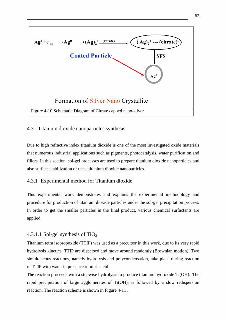
62
Figure 4-10 Schematic Diagram of Citrate capped nano-silver
4.3 Titanium dioxide nanoparticles synthesis
Due to high refractive index titanium dioxide is one of the most investigated oxide materials
that numerous industrial applications such as pigments, photocatalysis, water purification and
fillers. In this section, sol-gel processes are used to prepare titanium dioxide nanoparticles and
also surface stabilization of these titanium dioxide nanoparticles.
4.3.1 Experimental method for Titanium dioxide
This experimental work demonstrates and explains the experimental methodology and
procedure for production of titanium dioxide particles under the sol-gel precipitation process.
In order to get the smaller particles in the final product, various chemical surfactants are
applied.
4.3.1.1 Sol-gel synthesis of TiO2
Titanium tetra isopropoxide (TTIP) was used as a precursor in this work, due to its very rapid
hydrolysis kinetics. TTIP are dispersed and move around randomly (Brownian motion). Two
simultaneous reactions, namely hydrolysis and polycondensation, take place during reaction
of TTIP with water in presence of nitric acid.
The reaction proceeds with a stepwise hydrolysis to produce titanium hydroxide Ti(OH)4. The
rapid precipitation of large agglomerates of Ti(OH)4 is followed by a slow redispersion
reaction. The reaction scheme is shown in Figure 4-11 .

63
Hydrolysis: Ti(OC3H7)4 + 4H2O Ti(OH) 4 + 4C3H7OH
TTIP Titanium hydroxide Isopropanol
Polycondensation: Ti(OH) 4 TiO2 + 2H2O
Titanium hydroxide Titanium dioxide
Redispersion: TiO2 (Gel) nano-TiO2 (Sol)
Titanium dioxide Titanium dioxide
Figure 4-11 Reaction scheme for the preparation of nanosized Titanium dioxide
This process has been characterised by a rapid precipitation of large aggregates on a
millisecond time scale, followed by a slow redispersion (peptization) induced by the presence
of nitric acid and shear stress applying a turbulent hydrodynamic regime inside the stirred
tank reactor.
Production of nanosized titanium dioxide has been carried out on a laboratory scale using a
250 ml baffled, stirred batch reactor with confirmed standard configuration. The reaction
suspension has been stirred continuously (6-blade stirrer). The centre of the impeller has been
positioned at 1/3 height of the tank, the rotational speed has been measured. A thermostat has
been used to keep a constant temperature of 50° C inside of the batch reactor. For generating
titanium dioxide nanoparticles via a sol-gel process, the procedure is as follows.
A specified amount of 0.1 M nitric acid (HNO3) (141 ml.) is placed into the batch reactor. The
organic precursor titanium tetra isopropoxide 0.23 M TTIP (9.7 g) is added to the heated
solution under constant stirring at pH 1.3 as shown in Table 4-7.
Precipitation is observed to be occurring immediately due to the presence of dilute nitric acid
in the reaction mixture. Temperature is held constant for the rest of the redispersion reaction.
The variation of the stirrer speed is investigates the influence of turbulent hydrodynamic
conditions on particle size distribution and particle structure during reaction as shown in
Appendix A. The rotational speed of stirrer like 500, 750, 1000, and 1250 min-1
(shear rates
from =370 s-1
to =2515 s-1
) is chosen to be large in order to maximize redispersion of
agglomerates and to keep particles away from sedimentation settlement.
(50o C, pH=1.3)
(50o C, pH=1.3)
(50o C, pH=1.3)
0.1M HNO3
0.1M HNO3
0.1M HNO3
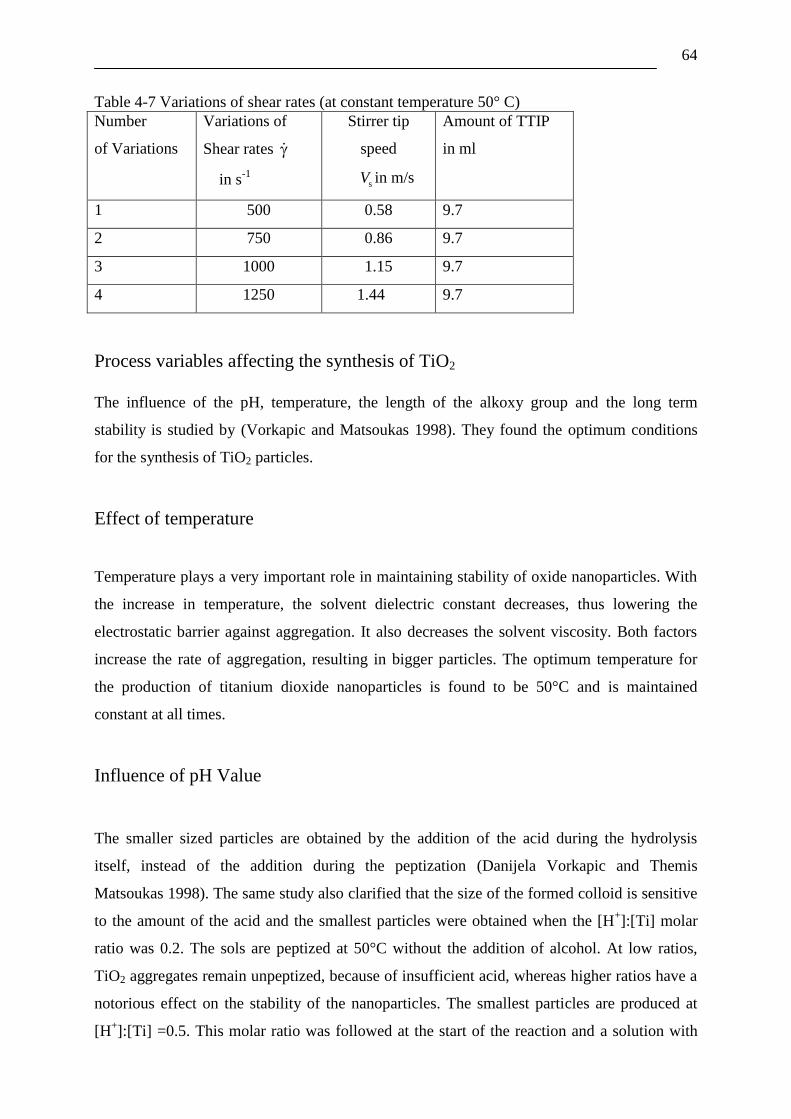
64
Table 4-7 Variations of shear rates (at constant temperature 50° C)
Number
of Variations
Variations of
Shear rates
in s-1
Stirrer tip
speed
sV in m/s
Amount of TTIP
in ml
1 500 0.58 9.7
2 750 0.86 9.7
3 1000 1.15 9.7
4 1250 1.44 9.7
Process variables affecting the synthesis of TiO2
The influence of the pH, temperature, the length of the alkoxy group and the long term
stability is studied by (Vorkapic and Matsoukas 1998). They found the optimum conditions
for the synthesis of TiO2 particles.
Effect of temperature
Temperature plays a very important role in maintaining stability of oxide nanoparticles. With
the increase in temperature, the solvent dielectric constant decreases, thus lowering the
electrostatic barrier against aggregation. It also decreases the solvent viscosity. Both factors
increase the rate of aggregation, resulting in bigger particles. The optimum temperature for
the production of titanium dioxide nanoparticles is found to be 50°C and is maintained
constant at all times.
Influence of pH Value
The smaller sized particles are obtained by the addition of the acid during the hydrolysis
itself, instead of the addition during the peptization (Danijela Vorkapic and Themis
Matsoukas 1998). The same study also clarified that the size of the formed colloid is sensitive
to the amount of the acid and the smallest particles were obtained when the [H+]:[Ti] molar
ratio was 0.2. The sols are peptized at 50°C without the addition of alcohol. At low ratios,
TiO2 aggregates remain unpeptized, because of insufficient acid, whereas higher ratios have a
notorious effect on the stability of the nanoparticles. The smallest particles are produced at
[H+]:[Ti] =0.5. This molar ratio was followed at the start of the reaction and a solution with

65
pH 1.2 was obtained. The suspension consists of small clusters that contain few primary
particles at this pH. The addition of the acid determines the long-term stability of the sol in
addition to the size of the colloid after peptization. After 5 days of experiments, the sols are
found to be unstable at high molar ratios and stable at optimum molar ratios, especially at 0.5.
Titanium nanoparticles can be stabilized electrostatically using acids or bases charging the
particle surface positively or negatively. Nanocolloid titanium dioxide is assumed to be stable
in the ranges of zeta potential between +20 mV to +40 mV in dependency with pH ranging
from 0.4 to 1.8 (Nikolov, Hintz et al. 2003).
Influence of alkoxides
Metal alkoxides are often dissolved in organic solvents before hydrolysis is performed.
Alkoxides are compounds with chemical formula M (OR)Z formed as a result of reactions
between metal M and alcohol, ROH. The relative performances of the alkoxides are studied
by (Danijela Vorkapic and Themis Matsoukas 2000). The temperature is maintained constant
throughout the process. Most commonly used solvents are parent alcohols, which have the
same number of carbon atoms as the metal alkoxide. However, it should be noted that
solvents are often not chemically inert toward metal alkoxides and that their reactivity can be
easily modified by changing the solvent (Harris and Byers 1988; Nabavi, Doeuff et al. 1990).
The alkoxides does not have a significant influence but Titanium isopropoxide is preferred
over others because of its high reactivity, and low electronegative value of titanium.
4.3.1.2 Surfactant based Titania nanoparticles
For the synthesis of surface stabilized TiO2 nanoparticles, titanium tetra isopropoxide (TTIP)
was used as precursor, nitric acid as stabilizer and different surfactants like PEG, EG and
NaCl are used in following section as shown in Table 4-8.
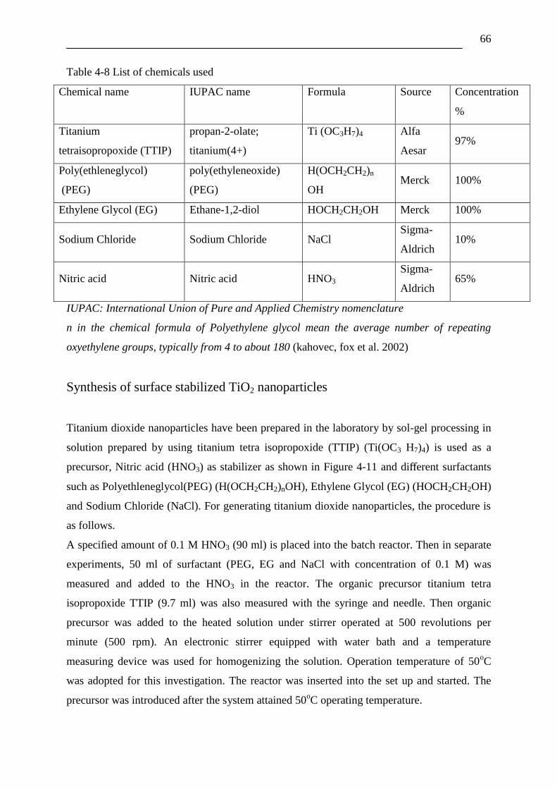
66
Table 4-8 List of chemicals used
Chemical name IUPAC name Formula Source Concentration
%
Titanium
tetraisopropoxide (TTIP)
propan-2-olate;
titanium(4+)
Ti (OC3H7)4 Alfa
Aesar 97%
Poly(ethleneglycol)
(PEG)
poly(ethyleneoxide)
(PEG)
H(OCH2CH2)n
OH Merck 100%
Ethylene Glycol (EG) Ethane-1,2-diol HOCH2CH2OH Merck 100%
Sodium Chloride Sodium Chloride NaCl Sigma-
Aldrich 10%
Nitric acid Nitric acid HNO3 Sigma-
Aldrich 65%
IUPAC: International Union of Pure and Applied Chemistry nomenclature
n in the chemical formula of Polyethylene glycol mean the average number of repeating
oxyethylene groups, typically from 4 to about 180 (kahovec, fox et al. 2002)
Synthesis of surface stabilized TiO2 nanoparticles
Titanium dioxide nanoparticles have been prepared in the laboratory by sol-gel processing in
solution prepared by using titanium tetra isopropoxide (TTIP) (Ti(OC3 H7)4) is used as a
precursor, Nitric acid (HNO3) as stabilizer as shown in Figure 4-11 and different surfactants
such as Polyethleneglycol(PEG) (H(OCH2CH2)nOH), Ethylene Glycol (EG) (HOCH2CH2OH)
and Sodium Chloride (NaCl). For generating titanium dioxide nanoparticles, the procedure is
as follows.
A specified amount of 0.1 M HNO3 (90 ml) is placed into the batch reactor. Then in separate
experiments, 50 ml of surfactant (PEG, EG and NaCl with concentration of 0.1 M) was
measured and added to the HNO3 in the reactor. The organic precursor titanium tetra
isopropoxide TTIP (9.7 ml) was also measured with the syringe and needle. Then organic
precursor was added to the heated solution under stirrer operated at 500 revolutions per
minute (500 rpm). An electronic stirrer equipped with water bath and a temperature
measuring device was used for homogenizing the solution. Operation temperature of 50oC
was adopted for this investigation. The reactor was inserted into the set up and started. The
precursor was introduced after the system attained 50oC operating temperature.
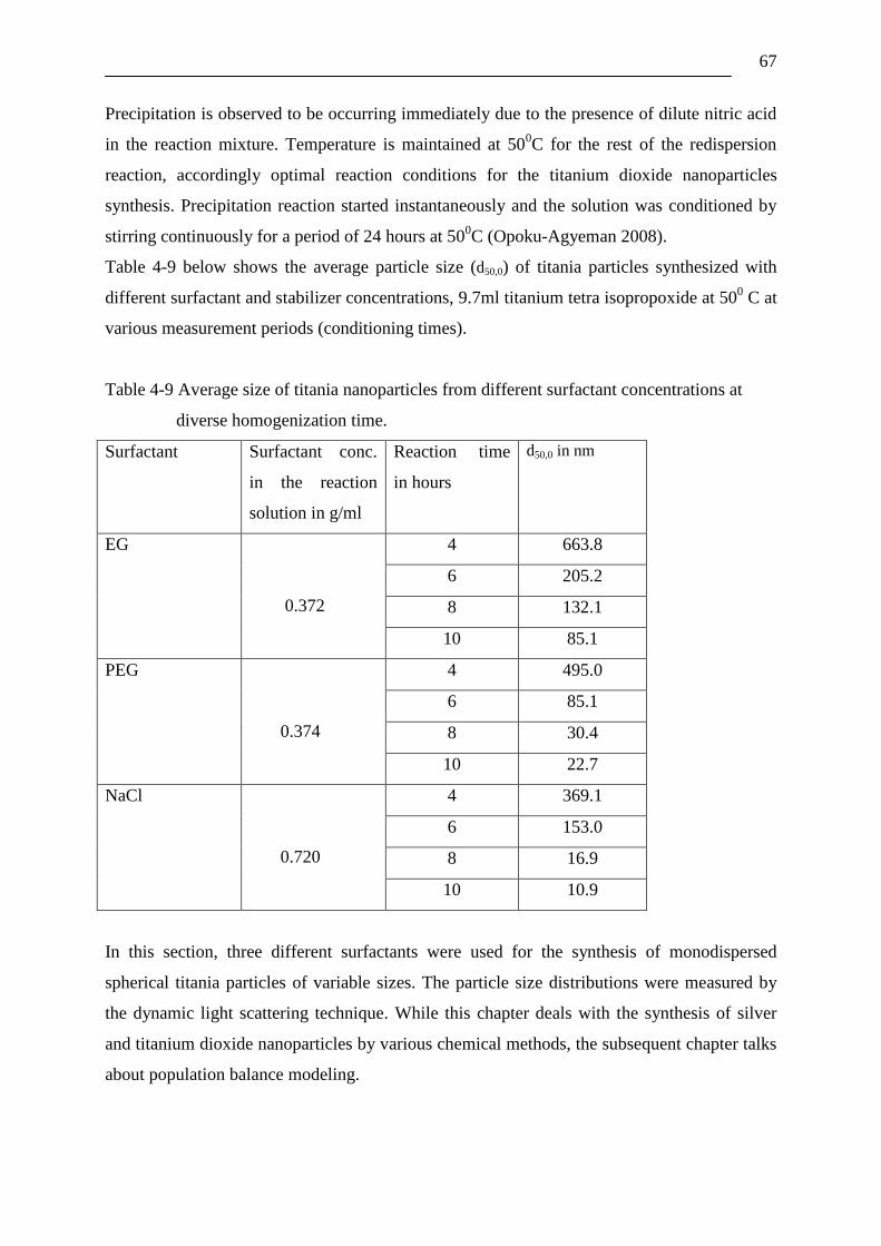
67
Precipitation is observed to be occurring immediately due to the presence of dilute nitric acid
in the reaction mixture. Temperature is maintained at 500C for the rest of the redispersion
reaction, accordingly optimal reaction conditions for the titanium dioxide nanoparticles
synthesis. Precipitation reaction started instantaneously and the solution was conditioned by
stirring continuously for a period of 24 hours at 500C (Opoku-Agyeman 2008).
Table 4-9 below shows the average particle size (d50,0) of titania particles synthesized with
different surfactant and stabilizer concentrations, 9.7ml titanium tetra isopropoxide at 500 C at
various measurement periods (conditioning times).
Table 4-9 Average size of titania nanoparticles from different surfactant concentrations at
diverse homogenization time.
Surfactant Surfactant conc.
in the reaction
solution in g/ml
Reaction time
in hours
d50,0 in nm
EG
0.372
4 663.8
6 205.2
8 132.1
10 85.1
PEG
0.374
4 495.0
6 85.1
8 30.4
10 22.7
NaCl
0.720
4 369.1
6 153.0
8 16.9
10 10.9
In this section, three different surfactants were used for the synthesis of monodispersed
spherical titania particles of variable sizes. The particle size distributions were measured by
the dynamic light scattering technique. While this chapter deals with the synthesis of silver
and titanium dioxide nanoparticles by various chemical methods, the subsequent chapter talks
about population balance modeling.

68
Chapter 5
Population Balance Modeling
“Make everything as simple as possible, but not simpler”
-Albert Einstein
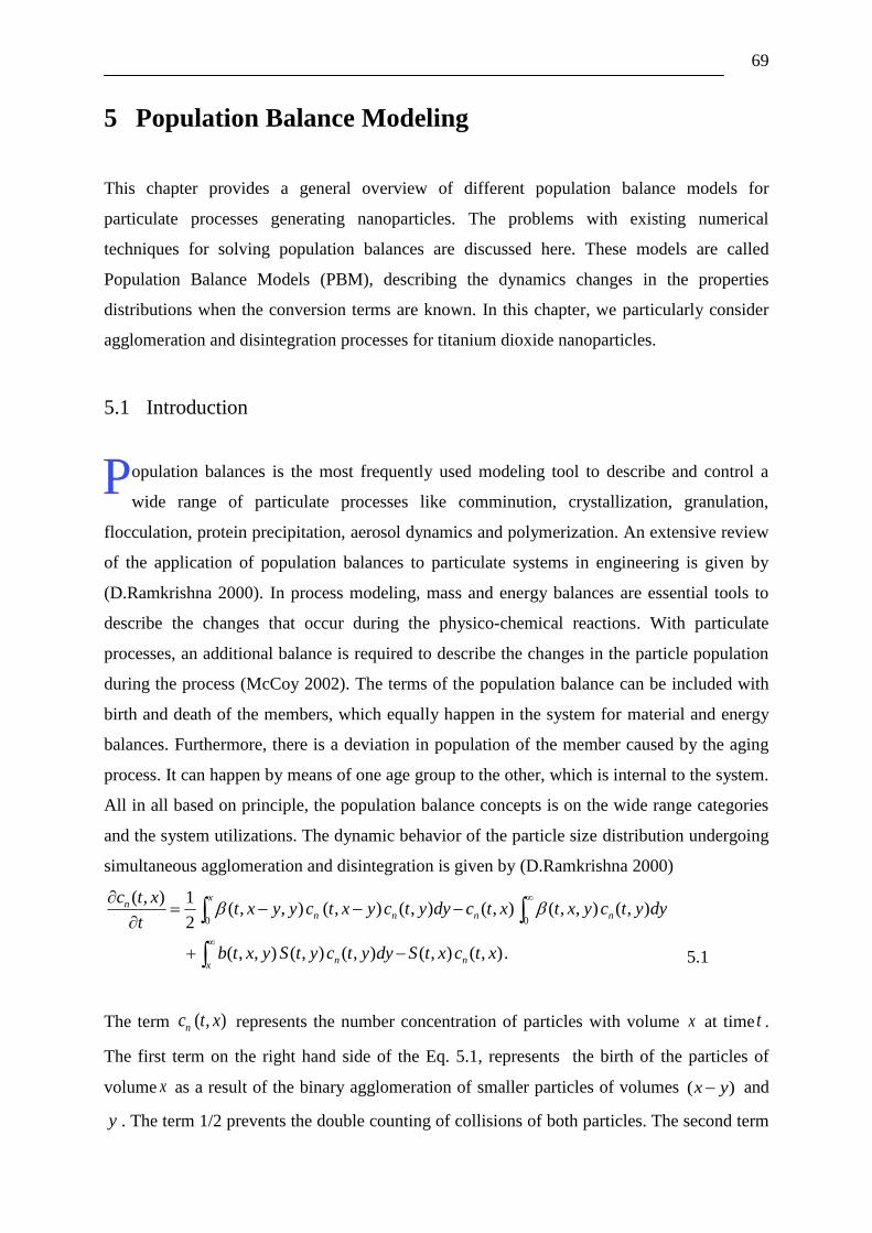
69
5 Population Balance Modeling
This chapter provides a general overview of different population balance models for
particulate processes generating nanoparticles. The problems with existing numerical
techniques for solving population balances are discussed here. These models are called
Population Balance Models (PBM), describing the dynamics changes in the properties
distributions when the conversion terms are known. In this chapter, we particularly consider
agglomeration and disintegration processes for titanium dioxide nanoparticles.
5.1 Introduction
opulation balances is the most frequently used modeling tool to describe and control a
wide range of particulate processes like comminution, crystallization, granulation,
flocculation, protein precipitation, aerosol dynamics and polymerization. An extensive review
of the application of population balances to particulate systems in engineering is given by
(D.Ramkrishna 2000). In process modeling, mass and energy balances are essential tools to
describe the changes that occur during the physico-chemical reactions. With particulate
processes, an additional balance is required to describe the changes in the particle population
during the process (McCoy 2002). The terms of the population balance can be included with
birth and death of the members, which equally happen in the system for material and energy
balances. Furthermore, there is a deviation in population of the member caused by the aging
process. It can happen by means of one age group to the other, which is internal to the system.
All in all based on principle, the population balance concepts is on the wide range categories
and the system utilizations. The dynamic behavior of the particle size distribution undergoing
simultaneous agglomeration and disintegration is given by (D.Ramkrishna 2000)
0 0
( , ) 1( , , ) ( , ) ( , ) ( , ) ( , , ) ( , )
2
( , , ) ( , ) ( , ) ( , ) ( , ).
xn
n n n n
n nx
c t xt x y y c t x y c t y dy c t x t x y c t y dy
t
b t x y S t y c t y dy S t x c t x
5.1
The term ( , )nc t x represents the number concentration of particles with volume x at time t .
The first term on the right hand side of the Eq. 5.1, represents the birth of the particles of
volume x as a result of the binary agglomeration of smaller particles of volumes ( )x y and
y . The term 1/2 prevents the double counting of collisions of both particles. The second term
P
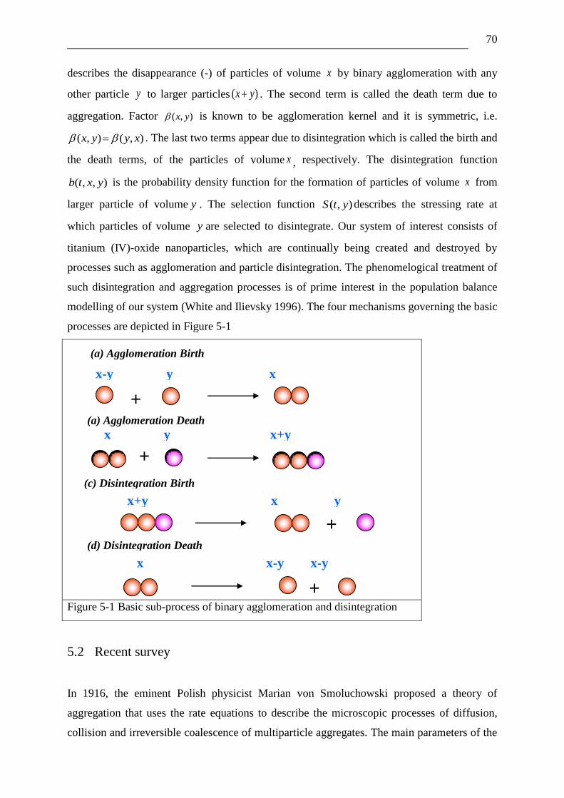
70
describes the disappearance (-) of particles of volume x by binary agglomeration with any
other particle y to larger particles ( )x y . The second term is called the death term due to
aggregation. Factor ( , )x y is known to be agglomeration kernel and it is symmetric, i.e.
( , ) ( , )x y y x . The last two terms appear due to disintegration which is called the birth and
the death terms, of the particles of volume x , respectively. The disintegration function
( , , )b t x y is the probability density function for the formation of particles of volume x from
larger particle of volume y . The selection function ( , )S t y describes the stressing rate at
which particles of volume y are selected to disintegrate. Our system of interest consists of
titanium (IV)-oxide nanoparticles, which are continually being created and destroyed by
processes such as agglomeration and particle disintegration. The phenomelogical treatment of
such disintegration and aggregation processes is of prime interest in the population balance
modelling of our system (White and Ilievsky 1996). The four mechanisms governing the basic
processes are depicted in Figure 5-1
Figure 5-1 Basic sub-process of binary agglomeration and disintegration
5.2 Recent survey
In 1916, the eminent Polish physicist Marian von Smoluchowski proposed a theory of
aggregation that uses the rate equations to describe the microscopic processes of diffusion,
collision and irreversible coalescence of multiparticle aggregates. The main parameters of the
+
+
+
+
(a) Agglomeration Birth
(c) Disintegration Birth
(d) Disintegration Death
x-y y x
x y x+y (a) Agglomeration Death
x+y x y
x x-y x-y
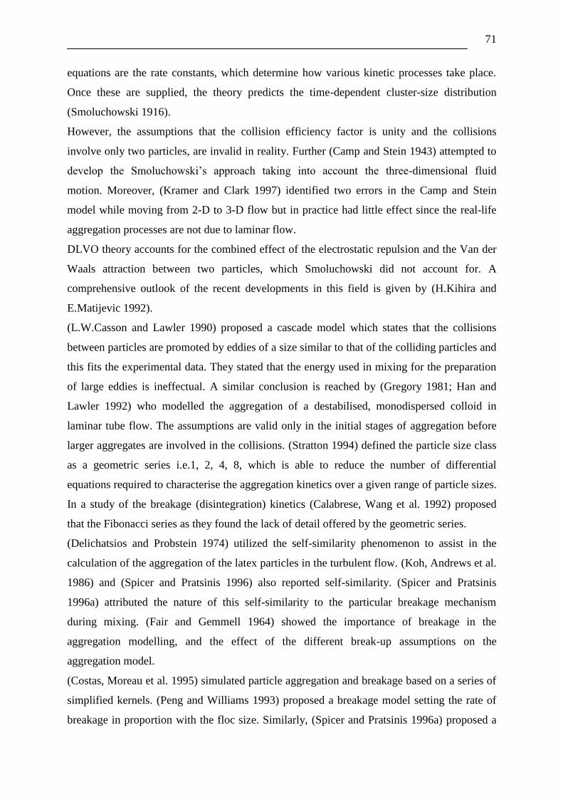
71
equations are the rate constants, which determine how various kinetic processes take place.
Once these are supplied, the theory predicts the time-dependent cluster-size distribution
(Smoluchowski 1916).
However, the assumptions that the collision efficiency factor is unity and the collisions
involve only two particles, are invalid in reality. Further (Camp and Stein 1943) attempted to
develop the Smoluchowski‟s approach taking into account the three-dimensional fluid
motion. Moreover, (Kramer and Clark 1997) identified two errors in the Camp and Stein
model while moving from 2-D to 3-D flow but in practice had little effect since the real-life
aggregation processes are not due to laminar flow.
DLVO theory accounts for the combined effect of the electrostatic repulsion and the Van der
Waals attraction between two particles, which Smoluchowski did not account for. A
comprehensive outlook of the recent developments in this field is given by (H.Kihira and
E.Matijevic 1992).
(L.W.Casson and Lawler 1990) proposed a cascade model which states that the collisions
between particles are promoted by eddies of a size similar to that of the colliding particles and
this fits the experimental data. They stated that the energy used in mixing for the preparation
of large eddies is ineffectual. A similar conclusion is reached by (Gregory 1981; Han and
Lawler 1992) who modelled the aggregation of a destabilised, monodispersed colloid in
laminar tube flow. The assumptions are valid only in the initial stages of aggregation before
larger aggregates are involved in the collisions. (Stratton 1994) defined the particle size class
as a geometric series i.e.1, 2, 4, 8, which is able to reduce the number of differential
equations required to characterise the aggregation kinetics over a given range of particle sizes.
In a study of the breakage (disintegration) kinetics (Calabrese, Wang et al. 1992) proposed
that the Fibonacci series as they found the lack of detail offered by the geometric series.
(Delichatsios and Probstein 1974) utilized the self-similarity phenomenon to assist in the
calculation of the aggregation of the latex particles in the turbulent flow. (Koh, Andrews et al.
1986) and (Spicer and Pratsinis 1996) also reported self-similarity. (Spicer and Pratsinis
1996a) attributed the nature of this self-similarity to the particular breakage mechanism
during mixing. (Fair and Gemmell 1964) showed the importance of breakage in the
aggregation modelling, and the effect of the different break-up assumptions on the
aggregation model.
(Costas, Moreau et al. 1995) simulated particle aggregation and breakage based on a series of
simplified kernels. (Peng and Williams 1993) proposed a breakage model setting the rate of
breakage in proportion with the floc size. Similarly, (Spicer and Pratsinis 1996a) proposed a
72
breakage model where the rate terms this time were assumed to be proportional to both the
floc size and the shear rate.
(Parker, Kaufman et al. 1972) studied the activated flocculation process using the model to
describe the changes of the settling characteristics. However, the model did not allow the
overall modelling of the settler. It only provided information about primary particles in the
supernatant (overflow) and effluent (underflow) suspended solids. In fact the sludge can be
viewed as a segregated population of individual flocs even though they are actual lump
biophase. The conversion terms are usually given as aggregation and redispersion (Nopens,
Biggs et al. 2002). They consider the flocs size as the floc property and the number
distribution based on floc size nc becomes
The main difference between Parker‟s models & PBM is the changes in the complete particle
size distribution. It is not considered only the fraction of the primary particles. The PBM has
been applied to various processes which are dealing with the particle or droplet populations.
In 2000, Biggs introduced another description to explain the activated sludge flocculation
process. He showed the PBM based on the aggregation model firstly led by (Hounslow, Ryall
et al. 1988). The main keywords for the aggregation and disintegration process are „birth‟ and
„death‟ of the flocs of the certain size. The number distribution of particle volumes vi due to
the four mechanisms of the two processes can be given by (Hounslow 1990; Nopens, Biggs et
al. 2002; Ding, Hounslow et al. 2006)
nAgg. Agg. Dist. Dist.
dc=B -D +B -D .
dt
5.3
The aggregation births BAgg and aggregation deaths DAgg in the above equation are given by
(Hounslow, Ryall et al. 1988). In order to get the solutions of such an integro-partial
differential equation, several numerical schemes are available based on space discretization.
The discretization divides the particle size range into a certain number of classes, which are
represented by floc size and volume.
ndc= Agglomeration- Disintegration
dt
5.2
73
5.3 Kinetics of the Simultaneous Agglomeration and Disintegration
Sub-Processes
Process engineers produce particulate materials such as powders and slurries by various
particulate processes such as milling, flocculation, precipitation and crystallization etc. In
these processes, the dispersed phase contains particles whose properties change in time and
space. It interacts with the continuous phase (air or liquid) which may be stationary, or in
motion, through mass transfer or chemical reactions.
For example, particles may become smaller via breakage due to mass transfer or chemical
reactions with the continuous phase. Similarly, the particles may become larger via
aggregation or growth due to mass transfer and chemical reaction with the continuous phase.
In general, the precipitation and crystallization processes consist of simultaneous
aggregation-disintegration processes, which means, the formed particles are continuously
agglomerated and disintegrated into the primary particles again.
5.3.1 Agglomeration Sub-Process
Aggregation or agglomeration is a process where two or more particles agglomerated form a
large particle. The total number of particles reduces in an aggregation process that shifts the
particle distribution towards larger sizes while mass remains conserved.
Agglomeration also may reduce the particle surface area for condensation and/or chemical
reaction. In general agglomeration phenomenon is very common in nature. For example
formation of snow flocs from a cloud of very fine ice cryptals. They are used to form larger
flocs falling due to the gravitational action. Coalescence occurs between bubbles or droplets
in a variety of dispersed phase systems in industrial processes, like waste water treatment,
food processing, and clinical diagnostics.
Agglomeration process is most common in powder processing industries. Agglomeration in
the fluidized bed takes place, if, after the drying of liquid bridges, solid bridges arise. There
are a large number of theoretical models available in the literature for predicting whether or
not two colliding particles stick together. These models involve a wide range of different
assumptions about the mechanical properties of the particles and the system characteristics.
The particles form aggregates as a result of collisions and these aggregates have higher
effective sizes than the primary particles, which build it. The increase in the effective size can
be explained by a typical example. The increase in the size of the aggregates accounts for the
removal of the particles in the layer of water above thermocline (a layer of water in an ocean

74
or certain lakes, where the temperature gradient is greater than that of the warmer layer above
and the colder layer below). Particles in lakes are in a continuous process of agglomeration
and disintegration until the steady state is reached. The final size depends on the shear rate
and the volume fraction. Also, agglomeration formation initiated in the atmosphere, induces
premature fallout of fine-grained ash. Hence, the settling velocity is higher for the
agglomeration than the dispersed ash particles.
In addition, agglomeration results in the modification of the effective surfaces of the particles.
This is important when they adhere pollutant particles with them. Aggregation reduces the
particle surface area for condensation and/or chemical reaction. This can have important
consequences for particle (e.g. aerosol or colloid) transport as larger particles settle more
rapidly under gravity but diffuse more slowly.
5.3.2 Disintegration Sub-Process
Disintegration means particle size reduction or particles disperse into primary particles.
Disintegration has a significant effect on the number of particles. The total number of
particles in a disintegration process increases while the total mass remains constant.
Disintegration process can be named as reversible agglomeration depending on the process
used. The term breakage denotes the mechanical fracture of the coarse solid. It can be applied
not only to systems in which solids undergo random breakage, but also to the mechanisms in
which the solids form from existing particles by other mechanisms. Also, cell division by
asexual means is an example of such process.
The breakage of a particle results from stressing at machine tools, or with other processes like
comminution operations. The particles distributed according to the mass or volume is
frequently used in process industries.
For these kinds of breakage processes, the size reduction of the solid material forms an
example. The evolution of drop size distributions in a stirred liquid-liquid dispersion in which
the dispersed fraction is small occurs mainly by drop breakage, since at the initial stages the
coalescence effects are negligibly small. The subject of high shear flows of colloidal
suspensions consisting of disintegrating the clusters of nanoparticles represents a vast field.
This is characterized by a wide spectrum of characteristic length and time scales. These shear
flows occur in a broad range of technological applications such as processing of
nanoparticles, and engineering disciplines. Ball milling, high shear mixing, or ultrasonication
are commonly used to disintegrate the agglomerate nanoparticles.
75
During ball milling, breakage occurs due to impact and high shear fields. The shape of
produced particles is irregular and many defects are introduced into the grain structure.
Efficiency of agglomeration and disintegration process depends on applied equipment and
process conditions.
5.3.3 The Moment Form of the Population Balance
The moments of the particle size distribution (PSD) can be obtained from writing it in terms
of moments. The jth moment of the particle size d is given as
0
, ( ) ( ) ( )
u
d
j
j r r
d
M d d q d d d 5.4
where ( )rq d is the frequency distribution of particle size d (J.Tomas 2007). If the internal
coordinate d is taken as length, then the zeroth moment is equal unity, and first, second, and
third moments are proportional to the averaged length, area and volume of particle collective,
respectively. On the other hand if d denotes volume of the particles, then the zeroth and first
moments are proportional to the total number and total mass of particles, respectively. The
second moment is in this case proportional to the light scattered by particles in the Rayleigh
limit(Kumar and Ramkrishna 1996). The moment forms of the population balance can be very
powerful.
5.4 Kernels of the Agglomeration and Disintegration Kinetics
In our model, agglomeration and disintegration takes place simultaneously. The primary
particles bind together to form agglomerates, while the agglomerates split into pieces, as
shown in Figure 5-1. The model is based on the assumption that the porous agglomerate
structure is formed with the nonporous primary particles.
5.4.1 Agglomeration rate kernel
Agglomeration, the growth of particles by collisions and subsequent bonding of smaller
particles contained in the fluid, can be alternatively called as aggregation or flocculation
according to the micro process used. Von Smoluchowski (Smoluchowski 1916) considered
the process of aggregation as a series of chemical reactions, and developed equations

76
describing the particle aggregation rates as well as expressions for the particle collisions in
solution (Park and Rogak 2004).
The mathematical representation of agglomeration has been based on the consideration that
the process consists of two micro processes: transport and adhesion. The transport step, which
leads to the collision of two particles, is achieved by the virtue of the local variations in
fluid/particle velocities arising through-
(1) Imposed velocity gradients from mixing (Orthokinetic agglomeration)
(2) The random thermal „Brownian‟ motion of the particles (Perikinetic agglomeration)
(3) Differences in the settling velocities of the individual particles (driven by forced field
of gravity or differential settling).
Adhesion is then, depending upon a number of short-range forces largely pertaining to the
nature of the surface themselves (Park and Rogak 2004).
The fundamental assumption of the aggregation process is that it is a second-order rate
constant process in which the rate of collision is the product of concentrations of the two
colliding particles. Mathematically, the rate of successful collisions between particles of size
,i jd d is given by,
Rate of collision ( , ) ,i j ni njr r c c 5.5
where is the agglomeration efficiency, ( , )i jr r is the collision frequency between particles
of radius ,i jr r and nic and njc are the particle concentrations for particles of radius ,i jr r ,
respectively.
The collision frequency is a function of the micro process, i.e. Perikinetic, orthokinetic or
differential sedimentation. The agglomeration efficiency gives (values from 0 to 1) is a
function of the probability of successful particle agglomeration events. In other words, larger
the agglomeration probability then value of is larger. Thus, in effect, is a measure of the
transport efficiency leading to collisions, while represents the percentage of those
collisions, which results in successful agglomeration events. All the models are based on this
one fundamental equation. The values of the parameters and are dependent upon the
nature of particles to the micro processes of agglomeration and the kinetic flow regime. The
research is devoted in finding the values for these two parameters and establishing equations.
Also the importance of nic and njc are noted, for the overall rate always increases with
particle concentration. The basic assumption is that the agglomeration rate is independent of
the colloidal interactions and depends only on the particle transport mechanism.

77
The assumption is based on the short-range nature of interparticle forces, which is usually
much less than the particle size, so that the particles come in contact before these forces play a
role. The decoupling of transport and adhesion steps is a strong simplification in the
agglomeration kinetics. At the moment, let us assume that every collision between the
particles results in the formation of an aggregate (i.e. the agglomeration efficiency, =1).
Hence, the agglomeration rate and the collision frequency are the same. Particle aggregation
can be described as by the rate at which a certain size aggregate is being formed by smaller
aggregates minus the rate at which the aggregate combines to form a larger aggregate from
small aggregates.
The rate of change of concentration of k -fold aggregates, where k i j , can be given by the
Smoluchowski equation as given in Eq.5.6
1
, ,
11
1,
2
i kn
i j ni nj nk i k ni
i j k ii
dcc c c c
dt
5.6
Where ,i j and k represent discrete fractions of particle sizes. The first term on the right hand
side represents the rate of formation of k -fold aggregates such that the total volume is equal
to the volume of the particle of size fraction k . The summation by this method means
counting each collision twice and hence the factor ½ is included. The second term on the right
hand side describes the loss of particles of size fraction k by virtue of their aggregation with
other particle sizes. The important notable point is that the above equation is applicable only
for irreversible aggregation since no term is included for the break-up of the aggregates,
which is usually common in aggregating environments.
5.4.2 Convection-Controlled Agglomeration
Mostly in practice the natural movement of the particles due to the Brownian motion is
insufficient to overcome the electrostatic repulsion barrier between the particles. This results
in permanent agglomeration. Nearly all the aggregation processes contain some form of
induced shear, due to laminar or turbulent fluid flow during stirring. The directional or
random movements of the particles due to the laminar or turbulent fluid flow during stirring
results in increase in the rate of interparticle collisions. Agglomeration resulting in this
manner is called as convection-controlled agglomeration, or orthokinetic agglomeration.
The main difference between the orthokinetic agglomeration and the perikinetic
agglomeration is the rate constants or kernels. In perikinetic agglomeration, as the
agglomeration proceeds, the big agglomerates move slowly when compared with the small

78
particles and hence there is reduction in the rate constant value. On the other hand, in the
orthokinetic agglomeration, as the size of agglomerates grows bigger, it tries to catch more
particles due to the shear and hence we observe increment in rate constant value. In short,
perikinetic agglomeration is more predominant in the initial stages of agglomerate
formation, while orthokinetic agglomeration wins the race in the later stages when the particle
size grows bigger.
5.4.2.1 Laminar Flow
The two extremes of flow pattern that can be considered are laminar and turbulent, which for
the sake of simplicity, can be associated with the ordered, directional and chaotic random
flow regimes with the reactor, respectively. Reynolds is the one who classified the flow into
laminar, transition and turbulent by a dimensionless equation as given below
2 2
Re a av D n
5.7
Where is av is the tip speed the stirrer, being the density of the fluid and is the viscosity
of the fluid. The term n is defined as the number of revolution of the stirrer; aD is the
impeller diameter and is the kinematic viscosity of the fluid. At low velocities, the flow is
laminar (Re 2100); there is no lateral mixing in this flow. At high velocities, the flow is
turbulent (Re 4000) which is marked by a chaotic nature. In between 2100 and 4000, the
transition regime exists (Patil, Andrews et al. 2001).
(Smoluchowski 1916) who considered only the case of uniform laminar shear did the first
work on the rate of orthokinetic aggregation. These conditions are more theoretical in nature
and seldom in practice but it is convenient to start with a simple case and then modify the
result for other conditions. Laminar and turbulent phenomena share the same kinetics for
agglomeration; the only difference is in the magnitude of the shear rates, , from the stirrer
power input. Here also the assumption is the same like Brownian diffusion, i.e. the diffusion
is due to the moving particle i to the fixed particle j (diffusion is due to the turbulent fluid
motion instead of the Brownian motion). Smoluchowski assumed that the particles flow in
straight streamlines and collide with other particles in different streamlines, according to their
relative position. The moving particles on streamlines that bring their center within a distance
i jr r (the collision radius, ijR ) of the central particle will collide (Collet 2004).The total

79
number of agglomeration events occurring between i and j particles in unit volume and unit
time is given by,
34
3ij ij ni nj ni nj i jJ c c c c r r
5.8
The constant for orthokinetic agglomeration can be written from the above equation as,
34
( , )3
i j i jr r r r 5.9
5.4.2.2 Turbulent Flow
We have considered so far the unrealistic situation of the uniform laminar shear. But, in the
actual process, the phenomenon of turbulence is the most dominated and needed one. In static
media, the aggregation of the nanoparticles is due to the Brownian collisions whereas the
larger particles settle due to gravity and have different settling velocities due to their sizes.
Therefore these collide and aggregate However, in many practical applications, it is necessary
to keep the solid-liquid suspension in motion to homogenize it. In such cases, in spite of the
flow pattern, the role of the local shear flow is dominant. The turbulent behavior of slurries in
a stirred tank is a typical example (Komarneni 2003). Moreover, turbulence is a poorly
understood phenomenon. Turbulence can be generated from contact of a flowing stream with
solid boundaries, called wall turbulence or from contact between layers of fluid moving at
different velocities called free turbulence (Patil, Andrews et al. 2001). Free turbulence is also
called as sheared flow.
Turbulent flow consists of a mass of eddies of various sizes existing along with each other in
the flowing stream. The continually forming large size eddies break into smaller eddies of
micro turbulence, and were dissipated into heat. The more vigor the turbulence has, the more
number of eddies are created. The eddies posses energy which is supplied by the potential
energy of the bulk flow of the fluid. From the energy point of view, turbulence transfers
energy from large eddies to smaller ones (micro turbulence).
The mechanical energy is not appreciably dissipated into heat during the breakup of the larger
eddies into smaller ones, and is worthless for practical purposes. This mechanical energy is
finally converted into heat as the micro eddies are dissipated. This energy transfer strongly
influences the particle transport and the particle agglomerations (Komarneni 2003). Camp and
Stein approached this problem in a stirred tank reactor by calculating the shear rate , from
the dissipation rates as power input per unit mass of the fluid, .
80
2
1
5.10
Where, is the kinematic viscosity of the fluid ( = ).
3 5
pN an D
V
5.11
Here, pN is the dimensionless power number; n is the number of revolutions; aD is the
impeller diameter and V is the volume of the reactor. The shear rate may be is inserted in
the Smoluchowski‟s equation to calculate the agglomeration events driven by turbulent
diffusion of fluid with a stirred tank reactor as shown in Eq.5.12
1
2 34
3ij i j ni njJ r r c c
5.12
The result is similar to the expression derived by (Saffman and Turner 1956) for particle
collisions in isotropic turbulence, but with a slightly different numerical factor.
5.4.3 Diffusion- Controlled Agglomeration
The agglomeration due to the continuous random movements of the tiny nanoparticles is
called diffusion-controlled agglomeration (also called as Perikinetic agglomeration)
(Smoluchowski 1917).
This is based on the assumption that every collision results in rapid agglomeration. This
agglomeration is solely due to the diffusion of the nanoparticles in the medium and the
diffusion coefficientiD of a spherical particle of radius
ir can be given by Stokes-Einstein
equation:
6
i
i
kTD
r
5.13
Where, k is Boltzman‟s constant, T is the absolute temperature, ir is the radius of the particle
and is the viscosity of the suspending fluid. The agglomeration rate of spherical
nanoparticles due to random, chaotic movements can be given as,
ij ij ni njJ c c 5.14
Here, ij is the agglomeration rate constant or agglomeration kernel. (Smoluchowski 1916)
Smoluchowski calculated the rates of diffusion of spherical particles of fraction i to a fixed
sphere j .
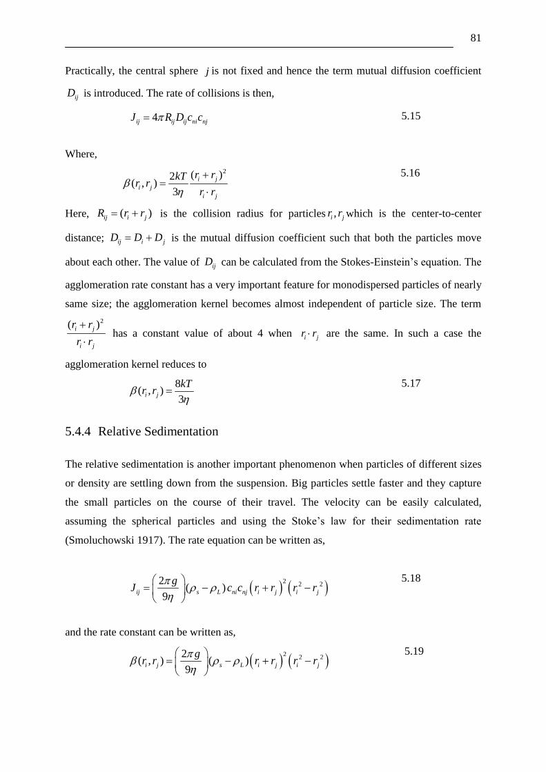
81
Practically, the central sphere j is not fixed and hence the term mutual diffusion coefficient
ijD is introduced. The rate of collisions is then,
4ij ij ij ni njJ R D c c 5.15
Where,
2( )2( , )
3
i j
i j
i j
r rkTr r
r r
5.16
Here, ( )ij i jR r r is the collision radius for particles ,i jr r which is the center-to-center
distance; ij i jD D D is the mutual diffusion coefficient such that both the particles move
about each other. The value of ijD can be calculated from the Stokes-Einstein‟s equation. The
agglomeration rate constant has a very important feature for monodispersed particles of nearly
same size; the agglomeration kernel becomes almost independent of particle size. The term
2( )i j
i j
r r
r r
has a constant value of about 4 when i jr r are the same. In such a case the
agglomeration kernel reduces to
8
( , )3
i j
kTr r
5.17
5.4.4 Relative Sedimentation
The relative sedimentation is another important phenomenon when particles of different sizes
or density are settling down from the suspension. Big particles settle faster and they capture
the small particles on the course of their travel. The velocity can be easily calculated,
assuming the spherical particles and using the Stoke‟s law for their sedimentation rate
(Smoluchowski 1917). The rate equation can be written as,
2
2 22( )
9ij s L ni nj i j i j
gJ c c r r r r
5.18
and the rate constant can be written as,
2
2 22( , ) ( )
9i j s L i j i j
gr r r r r r
5.19

82
Where, g is the acceleration due to gravity, and s is the density of the particles and L is the
density of the fluid. This phenomenon is important in the final stages of the agglomeration
where aggregate growth by sedimentation becomes dominant. But in our case, this
phenomenon can be neglected as the particles are of submicron size (M.Elimelech, Gregory et
al. 1995).
5.4.5 Effects of hydrodynamic interactions
The main assumption of the Smoluchowski theory is that the interparticle interactions are
negligible until the point of contact such that the collision takes place with 100% efficiency.
But, in reality the hydrodynamic forces are not negligible and they have a significant role
upon the colliding particles. When particles near each other to collide, the fluid in the space
between the particles is squeezed out. Hence, the particles rotate relative to one another, such
that they deviate from the linear path assumed in the Smoluchowski approach. This approach
is called as rectilinear approach (Danijela Vorkapic and Themis Matsoukas 1998).
Another alternative approach to this is the curvilinear approach, in which the hydrodynamic
forces cause the particle to rotate slightly around one another. The collision frequency
functions are also modified to incorporate for the hydrodynamic forces. In the following
Table 5-1, we summarized the different agglomeration kernels.
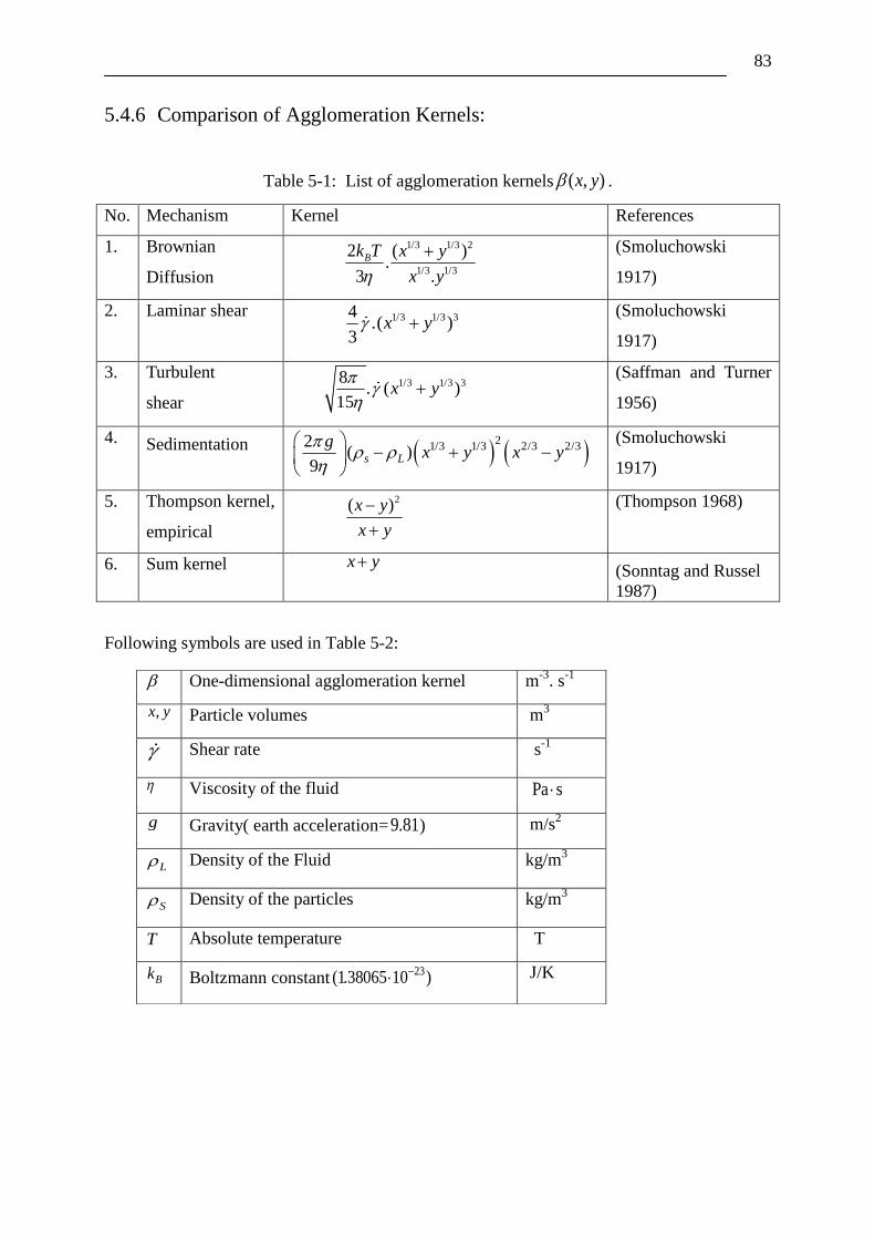
83
5.4.6 Comparison of Agglomeration Kernels:
Table 5-1: List of agglomeration kernels ( , )x y .
No. Mechanism Kernel References
1. Brownian
Diffusion
1/3 1/3 2
1/3 1/3
2 ( ).
3 .
Bk T x y
x y
(Smoluchowski
1917)
2. Laminar shear 1/3 1/3 34.( )
3x y
(Smoluchowski
1917)
3. Turbulent
shear
1/3 1/3 38. ( )
15x y
(Saffman and Turner
1956)
4. Sedimentation
21/3 1/3 2/3 2/32
( )9
s L
gx y x y
(Smoluchowski
1917)
5. Thompson kernel,
empirical
2( )x y
x y
(Thompson 1968)
6. Sum kernel x y (Sonntag and Russel
1987)
Following symbols are used in Table 5-2:
One-dimensional agglomeration kernel m-3
. s-1
,x y Particle volumes m3
Shear rate s-1
Viscosity of the fluid Pa s
g Gravity( earth acceleration=9.81) m/s2
L Density of the Fluid kg/m3
S Density of the particles kg/m3
T Absolute temperature T
Bk Boltzmann constant23(1.38065 10 ) J/K
84
5.4.7 Disintegration rate kernel
Disintegration is usually first order with respect to particle concentration, This means, the
larger the particle fraction concentration within the process chamber of a reactor the larger is
the proability of stressing and as its results of disintegration or breakage. But it is dependent
on the local hydrodynamic field acting on the particles. However, it is the balancing of
opposing phenomena of agglomeration called redispersion that decides the agglomerate size.
The computer simulations of (Fair and Gemmell 1964) showed the importance of redisper-
sion or breakage in the agglomeration modeling.
Different researchers have proposed different disintegration functions ( , , )b t x y or probability
density functions. The particle disintegration and breakage based on a series of different
simplified kernels assumes that the initial particle size distribution is monodispersed or
narrow distributed. The results show that the different assumptions can have effect on both
the initial rates of reaction and the steady state concentrations (Spicer and Pratsinis
1996a).The disintegration rate is assumed to be a function of the particle volume (Pandya and
Spielman 1982),
0( ) ( )S x S x 5.20
where =1/3 (Boadway 1978), consistent with the expectation that the breakage rate is
proportional to the particle size x . The Selection rate for disintegration S has been used for
flow shear rate as the essential stressing parameter. The break up rate coefficient can be
expressed as (Kim and Kramer 2006),
( ) ( )f
i iS A r 5.21
The term iS is the selection rate for disintegration, A is the disintegration rate constant, ir is
the particle radius, and f are the fit parameter from experimental data and is the shear
rate. This shows that the selection rate for disintegration is a function of flow strain rate
resulting from energy input and the geometric properties of the agglomerate (i.e. size, area, or
volume).
Over the last many years several attempts have been made to model disintegration kernel. In
the following sections different forms of disintegration kernels are discussed.
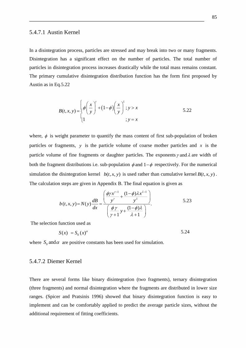
85
5.4.7.1 Austin Kernel
In a disintegration process, particles are stressed and may break into two or many fragments.
Disintegration has a significant effect on the number of particles. The total number of
particles in disintegration process increases drastically while the total mass remains constant.
The primary cumulative disintegration distribution function has the form first proposed by
Austin as in Eq.5.22
1 ;
( , , )
1 ;
x xy x
B t x y y y
y x
5.22
where, is weight parameter to quantify the mass content of first sub-population of broken
particles or fragments, y is the particle volume of coarse mother particles and x is the
particle volume of fine fragments or daughter particles. The exponents and are width of
both the fragment distributions i.e. sub-population and 1 respectively. For the numerical
simulation the disintegration kernel ( , , )b t x y is used rather than cumulative kernel ( , , )B t x y .
The calculation steps are given in Appendix B. The final equation is given as
1 1(1 )
( , , ) ( ) .(1 )
1 1
x x
y ydBb t x y N y
dxy
5.23
The selection function used as
0( ) ( )S x S x 5.24
where 0 andS are positive constants has been used for simulation.
5.4.7.2 Diemer Kernel
There are several forms like binary disintegration (two fragments), ternary disintegration
(three fragments) and normal disintegration where the fragments are distributed in lower size
ranges. (Spicer and Pratsinis 1996) showed that binary disintegration function is easy to
implement and can be comfortably applied to predict the average particle sizes, without the
additional requirement of fitting coefficients.

86
Here we employed Diemer's generalized form of Hill and Ng's power-law breakage
distribution (Diemer and Olson 2002) as in Eq.5.25
( 1)( -2)
( -1)
( - ) ( 1)( -1) !( , )
! ( 1)( - 2) !
c c c p
pc p
p x y x c c pb x y
y c c c p
5.25
Here, the exponent p describes the number of fragments per disintegration event and 0c
determines the shape of the daughter particle distribution. In the following Table 5-3, we
summarized the different disintegration kernels.

87
5.4.8 Comparison of Disintegration Kernels
Table 5-3: List of disintegration kernels.
No. Mechanism Kernels References
1 Austin
kernel 1 ;( , , )
1 ;
x xy x
B t x y y y
y x
(Austin 2002)
2 Diemer kernel
( 1)( -2)
( -1)
( - ) ( 1)( -1) !( , )
! ( 1)( - 2) !
c c c p
pc p
p x y x c c pb x y
y c c c p
(Diemer and Olson
2002)
3 Kramer Kernel
( ) ( )fA x (Kramer and Clark
1997)
4 Power law
Kernel
x (A.D.Randolph
1969)
Following symbols are used in Table 5-4:
b Disintegration kernel m
-3
B Cumulative disintegration kernel -
,x y Particle volumes m3
f Fit parameter from experimental data -
width of the fragment distributions -
Dimensionless material constant -
Fraction of sub population of fines -
Fit parameter from experimental data -
p Number of fragments per single
disintegration event
-
c Shape of the daughter particle distributions -

88
5.5 Methods to Solve the Population Balance Equations
Analytical solutions for agglomeration disintegration population balance equations are
available only for a limited number of simplified problems and therefore numerical solutions
are frequently needed to solve such equations. Sectional methods such as Cell Average
Technique (CAT) and Fixed Pivot Technique (FVT) are used to solve population balances.
Several numerical techniques including the method of successive approximations
(D.Ramkrishna 2000), the method of moments (Barrett and Jheeta 1996; Mahoney and
Ramkrishna 2002), the finite element methods (Nicmanis and Hounslow 1996; Mahoney and
Ramkrishna 2002), the finite volume schemes (Motz, Mitrovic et al. 2002; Verkoeijen, A.
Pouw et al. 2002; Filbet and Laurencot 2004) and Monte Carlo simulation methods (F. Einar
Kruis, Arkadi Maisels et al. 2000; Lin, Lee et al. 2002; Maisels, Einar Kruis et al. 2004) can
be found in the literature for solving PBEs.
Population balance equations related to agglomeration and disintegration can be expressed by
continuous and discrete approaches. Some analytical solutions are available under certain
conditions on kernels (Peterson 1986; Ziff 1991). Therefore, numerical solutions are required
for these agglomeration disintegration models. The simultaneous agglomeration disintegration
in the form of a continuous population balance equations can be shown by Eq. 5.26
max
min min
max
( , ) 1( , , ) ( , ) ( , ) ( , ) ( , , ) ( , )
2
( , , ) ( , ) ( , ) ( , ) ( , )
x xn
n n n nx x
x
n nx
c t xt x y y c t x y c t y dy c t x t x y c t y dy
t
b t x y S t y c t y dy S t x c t x
5.26
In all population balance equations mentioned above, the size variable may vary from 0 to ∞.
In order to apply a numerical scheme for the solution of the equation the first step is to fix a
finite computational domain. Therefore, we consider truncated equations by replacing ∞ by a
sufficiently large size maxx , with maxx and we also define min 0x . Furthermore, for the
sake of simplicity we assume that the kernels are compact enough so that the total mass of the
system remains conserved.
5.5.1 Numerical Methods
The different sectional methods are differ mainly in terms of freedom of discretization, grid
choice and conserved properties (at least two) during the discretization. The division in a
number of certain size fractions is well known in process engineering because they are simple
to implement and produce exact numerical results of some selected properties.
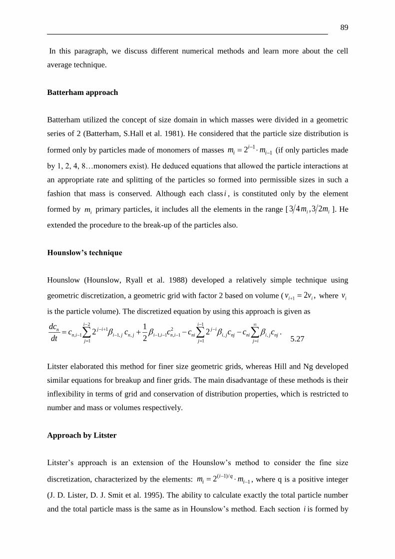
89
In this paragraph, we discuss different numerical methods and learn more about the cell
average technique.
Batterham approach
Batterham utilized the concept of size domain in which masses were divided in a geometric
series of 2 (Batterham, S.Hall et al. 1981). He considered that the particle size distribution is
formed only by particles made of monomers of masses 1
12ii im m
(if only particles made
by 1, 2, 4, 8…monomers exist). He deduced equations that allowed the particle interactions at
an appropriate rate and splitting of the particles so formed into permissible sizes in such a
fashion that mass is conserved. Although each class i , is constituted only by the element
formed by im primary particles, it includes all the elements in the range [ ii mm 23,43 ]. He
extended the procedure to the break-up of the particles also.
Hounslow’s technique
Hounslow (Hounslow, Ryall et al. 1988) developed a relatively simple technique using
geometric discretization, a geometric grid with factor 2 based on volume ( ,21 ii vv where iv
is the particle volume). The discretized equation by using this approach is given as
2 11 2
, 1 1, , 1, 1 , 1 , ,
1 1
12 2 .
2
i ij i j in
n i i j n j i i n i ni i j nj ni i j nj
j j j i
dcc c c c c c c
dt
5.27
Litster elaborated this method for finer size geometric grids, whereas Hill and Ng developed
similar equations for breakup and finer grids. The main disadvantage of these methods is their
inflexibility in terms of grid and conservation of distribution properties, which is restricted to
number and mass or volumes respectively.
Approach by Litster
Litster‟s approach is an extension of the Hounslow‟s method to consider the fine size
discretization, characterized by the elements: ( 1)/
12 i qi im m
, where q is a positive integer
(J. D. Lister, D. J. Smit et al. 1995). The ability to calculate exactly the total particle number
and the total particle mass is the same as in Hounslow‟s method. Each section i is formed by

90
the particles in the range
i
q
iq
q
mm2
21,
2.2
211
1
1
, hence the method reduces to Hounslow‟s
model when q=1. If applied to discrete size distributions with q1, it creates a number of
fractions, which contains no particle. This approach is not suited for the inclusion of breakup
and it should be coupled with some other method to treat agglomeration-fragmentation
processes.
Approach by Marchal
Marchal considered the process of aggregation as a chemical reaction whose stoichiometric
coefficients can be adjusted for mass conservation (Marchal, David et al. 1988). The particle
size distribution is divided into h arbitrary fractions, whose boundary elements are formed by
'
im monomers. Any section i includes all the particles made by a number of monomers in the
range [''
1 , ii mm ], i =1, 2…h. The element of mass
'
im can be the representative element of
section , ii m . Better accuracy can be obtained with the arithmetic mean: 2/)( ''
1 iii mmm
Marchal claimed that the method can be applied to the breakup as well, provided that only
two fragments are formed, but there is no explicit formulation available. When dealing with
probability density function, this lacks adequacy.
Approach by Vanni
Vanni proposed a system of sectional representation for pure fragmentation systems, in which
sections of arbitrary size is used (Vanni 2000). The section boundaries contain the elements
,'im i =0, 1, 2…h, and the representative element of each section is im . The only restriction
on the choice of im is, of course, that''
1 iii mmm .
The fixed pivot technique (FPT)
The main disadvantage of the above described discretization techniques is that they can be
used for limited number of geometric grids. (Kumar and Ramkrishna 1996) proposed a new
method called fixed pivot technique. PBE can be solved for any arbitrarily chosen grids by
using the fixed pivot technique. In this method, they find the position of new born particles

91
i.e. v and u
in our case as shown in Figure 5-2 and then distribute it between two
neighboring nodes. However, the difficulty arises when this new born particle does not
coincide with one of the existing grid or pivots points. In such cases particles are reallocated
to the adjacent pivots (as in Figure 5-2) in such a way that two arbitrarily chosen properties
number and mass of the distribution are conserved. The set of equations required to conserve
both mass and numbers are given by
, , , ,
,
11
2 j k i k
j k
ij k i x x j k i x x k i k i j i i
j k k kj i
dNN N N N S x N S x N
dt
5.28
where, iN is the total number of particles in the i th size range at time t and is given as
1
( , )i
i
x
i n
x
N c t x dx
and
1
1
1
1
1
1
( )when ( )
( )when ( )
i j k
i j k i
i i
i
j k i
i j k i
i i
x x xx x x x
x x
x x xx x x x
x x
5.29
1
1
1 1,
1 1
( , ) ( , ) .i i
i i
x x
i ii k k k
i i i ix x
x y y xb y x dy b y x dy
x x x x
5.30
Figure 5-2 Rearrangement of newly formed particles that do not coincide with an existing
pivot: Fixed pivot
Eq.5.28 consist of four terms. The first is the aggregation birth term and contains a
factor responsible for the reallocation of the formed particles to the adjoining pivots if
they do not coincide with a pivot. The second term describes the loss of particles due to
aggregation (aggregation death) and does not require any reallocation since particles only
92
disappear and are not formed. The third term (breakage birth) does require a factor for
reallocation ( ,i k ) based on the breakage distribution function (Eq.5.30). The fourth term
describes the loss of particles due to breakup (breakage death) and since no particles are
formed during this process this term also does not require any reallocation.
Note that, when a geometrical grid with factor 2 (volume-based) is used, Eqs.5.28 and
5.29 are the simplified equations that can only be used to conserve numbers and mass and
will, hence, yield identical results as the ones derived by (Hounslow, Ryall et al. 1988).
The advantage of the fixed pivot technique is its generality in terms of the properties to
be conserved and the grid choice. The predictions for the cases involving simultaneous
agglomeration and breakage suffered from severe over predictions in the large particle
size range.
5.5.2 Cell Average Technique- CAT
This section summarizes the newly developed numerical method cell average technique
(CAT) for solving population balances (Kumar 2006). This method approximates the number
density in terms of Dirac point masses and is based on an exact prediction of some selected
moments to solve the population balance equation. The objective behind the cell average
technique is to divide the entire size domain into a finite number of cells. The lower and upper
boundaries of the i th cell are denoted by i 1/ 2x and i 1/ 2x , respectively. All particles belonging
to a cell are identified by a representative size in the cell, also called grid point. The
representative size of a cell can be chosen at any position between the lower and upper
boundaries of the cell. A typical discretized size domain is shown in Figure 5-3.The
representative of the i th cell is represented by i i 1/2 i 1/2x (x x ) / 2 and the width of the i th
cell is denoted by i i 1/ 2 i 1/ 2x x x . The size of a cell can be fixed arbitrarily depending upon
the process of application. In most applications, however, geometric type grids are preferred.
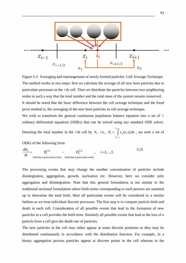
93
Figure 5-3 Averaging and rearrangement of newly formed particles: Cell Average Technique
The method works in two steps: first we calculate the average of all new born particles due to
particulate processes in the i th cell. Then we distribute the particles between two neighboring
nodes in such a way that the total number and the total mass of the system remain conserved.
It should be noted that the basic difference between the cell average technique and the fixed
pivot method is, the averaging of the new born particles in cell average technique.
We wish to transform the general continuous population balance equation into a set of I
ordinary differential equations (ODEs) that can be solved using any standard ODE solver.
Denoting the total number in the i th cell by iN , i.e., 1/2
1/2
( , )i
i
x
i n
x
N c t x dx
, we seek a set of
ODEs of the following form
CA CAii i
birth due to particulateevents death due to particulateevents
dNB D , i 1,..., I.
dt
5.31
The processing events that may change the number concentration of particles include
disintegration, aggregation, growth, nucleation etc. However, here we consider only
aggregation and disintegration. Note that this general formulation is not similar to the
traditional sectional formulation where birth terms corresponding to each process are summed
up to determine the total birth. Here all particulate events will be considered in a similar
fashion as we treat individual discrete processes. The first step is to compute particle birth and
death in each cell. Consideration of all possible events that lead to the formation of new
particles in a cell provides the birth term. Similarly all possible events that lead to the loss of a
particle from a cell give the death rate of particles.
The new particles in the cell may either appear at some discrete positions or they may be
distributed continuously in accordance with the distribution function. For example, in a
binary aggregation process particles appear at discrete points in the cell whereas in the
94
disintegration process they are often distributed everywhere according to a continuous
disintegration function.
Let us demonstrate the basic concepts of the cell average technique by the following example.
The number of particle births iI1 2
i i iB ,B ,...,B take place at positions iI1 2
i i iy , y ,..., y , somewhere
in discretized domain, due to some particulate processes like aggregation, disintegration in the
cell i . Here we consider the purely discrete case but analogous steps can be performed for
continuous appearance of the particles in the cell. First we compute the average number of
birth of the particles in the i th cell as
Ii ji i
j 1
B B
5.32
Since we know the positions of the newborn particles inside the cell, it is easy to calculate the
average birth of newborn particles iv . It is given by the following formula
Ii j ji i
j 1
i
i
y B
vB
5.33
Now we may assume that iB particles are sitting at the position iv . It should be noted that the
averaging process still maintains consistency with respect to the first two moments. If the
average volume iv matches with the representative size ix then the total birth
iB can be
assigned to the nodeix . But this is rarely possible and hence the average fraction iv has to be
reassigned to the neighboring nodes such that the total number and mass remain conserved.
Considering that the average volumei iv x , the assignment of particles must be performed
by considering the following equations
1 i i 2 i i+1 i
i 1 i i i+1 2 i i+1 i i
a (v , x )+a (v ,x )= B ,
x a (v ,x )+x a (v ,x )= B v .
5.34
Here 1 i ia (v , x ) and
2 i i 1a (v , x ) are the number fractions of the birth
iB to be assigned at ix
and i 1x ,
respectively. Solving the above equations we obtain
+i i+11 i i i i i i
i i+1
-i i2 i i+1 i i i+1 i
i+1 i
v -xa (v ,x )=B =B λ (v ),
x -x
v -xa (v ,x )=B =B λ (v ),
x -x
5.35
95
where
i 1
ii i 1
x x(x)
x x
5.36
There are 4 possible birth fractions that may add a birth contribution at the node ix : two from
the neighboring cells and two from the i th cell. Collecting all the birth contributions, the birth
term for the cell average technique is given by
CA - -i i-1 i i-1 i-1 i-1 i i i i i
+ +i i i i i i+1 i i+1 i+1 i+1
B = B λ (v )H(v -x )+B λ (v )H(x -v )
+B λ (v )H(v -x )+B λ (v )H(x -v ).
5.37
Here, H is the Heaviside step function which is a discontinuous function also known as unit
step function and is defined by
1, x>0
1H(x)= , x=0
2
0, x<0
5.38
where x is an arbitrary variable.
Substituting the values of CA
iB and CA
iD into the Eq. 5.31, we obtain a set of ordinary
differential equation. It will be then solved by any higher order ODE solver. Note that there is
no need to modify the death term since particles are just removed from the grid points and
therefore the formulation remains consistent with all moments due to the discrete death. As a
result the death term CA
iD in the cell average formulation is equal to the sum of total death in
the i th cell. For the detailed description of the scheme, readers are referred to (Kumar 2006;
Kumar, Peglow et al. 2008). The next chapter explains the numerical simulation by using the
cell average technique and comparing it with the experimental results.
96
Chapter 6
Experimental and Modeling Results
“No problem is too small or too trivial if we can really do something about it”
-Richard Feynman
97
6 Experimental and Modeling Results
In this chapter, we discuss: first the synthesis of silver nanoparticles by double reduction
method and second the agglomeration and disintegration process of titanium dioxide
nanoparticles synthesized by sol-gel process.
The prime goal is the optimization of nanoparticles formation process in the liquid phase with
different conditions. Silver and titanium dioxide nanoparticles are produced in the batch
reactor. They are investigated both by experimentally as well as by simulations based on the
population balance equations. The population balance models for agglomeration and
disintegration leads to a system of integro-partial differential equations, which can be
numerically solved by several numerical schemes. Here the cell average technique is used to
solve PBEs and predict the particle size distributions and moments.
6.1 Experimental results of silver nanoparticles
ynthesis of silver nanoparticles is done by double reduction method. In this process silver
particles are capped with citrate ions and then it is reduced by sodium formaldehyde
sulphoxylate. In general surface capped silver powder can be effectively converted to
colloidal state via re-dispersion. Here, the agglomeration process is caused by rapid collision
of the particles and their afterward bonding. Depending on their interactions, this collision
results in the agglomeration or redispersion of particles. During the time of the process, after
the drop wise addition of reducing agent the redispersion begins and then the particle size
distribution develops rapidly. The size of the particles distribute into the wide and varied
range. Particle size distribution and zeta potential were measured using Dynamic Light
scattering method (DLS). Results obtained with all the experiments performed are
summarized in tables and graphical representations in this section.
6.1.1 Effect of Capping Agent
In this work, the capping of silver particles by tri-sodium citrate is investigated under different
conditions. Citrate is an efficient stabilizer. All the solutions were clear and stable for weeks
in absence of air. Capping agents when present inhibit the growth of nanoparticles by
passivating their surfaces. The synthesis of almost all the nanoparticles is done in the presence
of capping agents in order to stabilize the size of nanoparticles for a desired application.
S
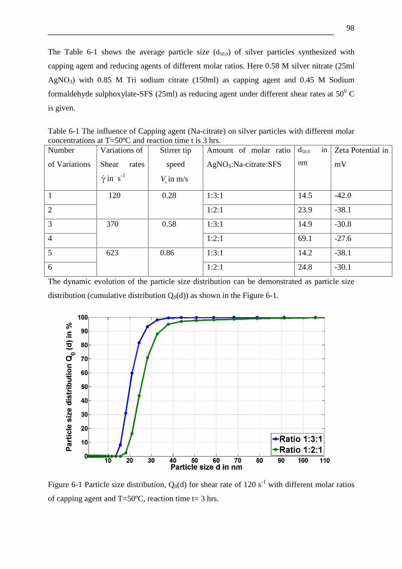
98
The Table 6-1 shows the average particle size (d50,0) of silver particles synthesized with
capping agent and reducing agents of different molar ratios. Here 0.58 M silver nitrate (25ml
AgNO3) with 0.85 M Tri sodium citrate (150ml) as capping agent and 0.45 M Sodium
formaldehyde sulphoxylate-SFS (25ml) as reducing agent under different shear rates at 500 C
is given.
Table 6-1 The influence of Capping agent (Na-citrate) on silver particles with different molar
concentrations at T=50ºC and reaction time t is 3 hrs.
Number
of Variations
Variations of
Shear rates
in s-1
Stirrer tip
speed
sV in m/s
Amount of molar ratio
AgNO3:Na-citrate:SFS
d50,0 in
nm
Zeta Potential in
mV
1 120
0.28 1:3:1 14.5 -42.0
2 1:2:1 23.9 -38.1
3 370 0.58 1:3:1 14.9 -30.8
4 1:2:1 69.1 -27.6
5 623 0.86 1:3:1 14.2 -38.1
6 1:2:1 24.8 -30.1
The dynamic evolution of the particle size distribution can be demonstrated as particle size
distribution (cumulative distribution Q0(d)) as shown in the Figure 6-1.
Figure 6-1 Particle size distribution, Q0(d) for shear rate of 120 s-1
with different molar ratios
of capping agent and T=50ºC, reaction time t= 3 hrs.
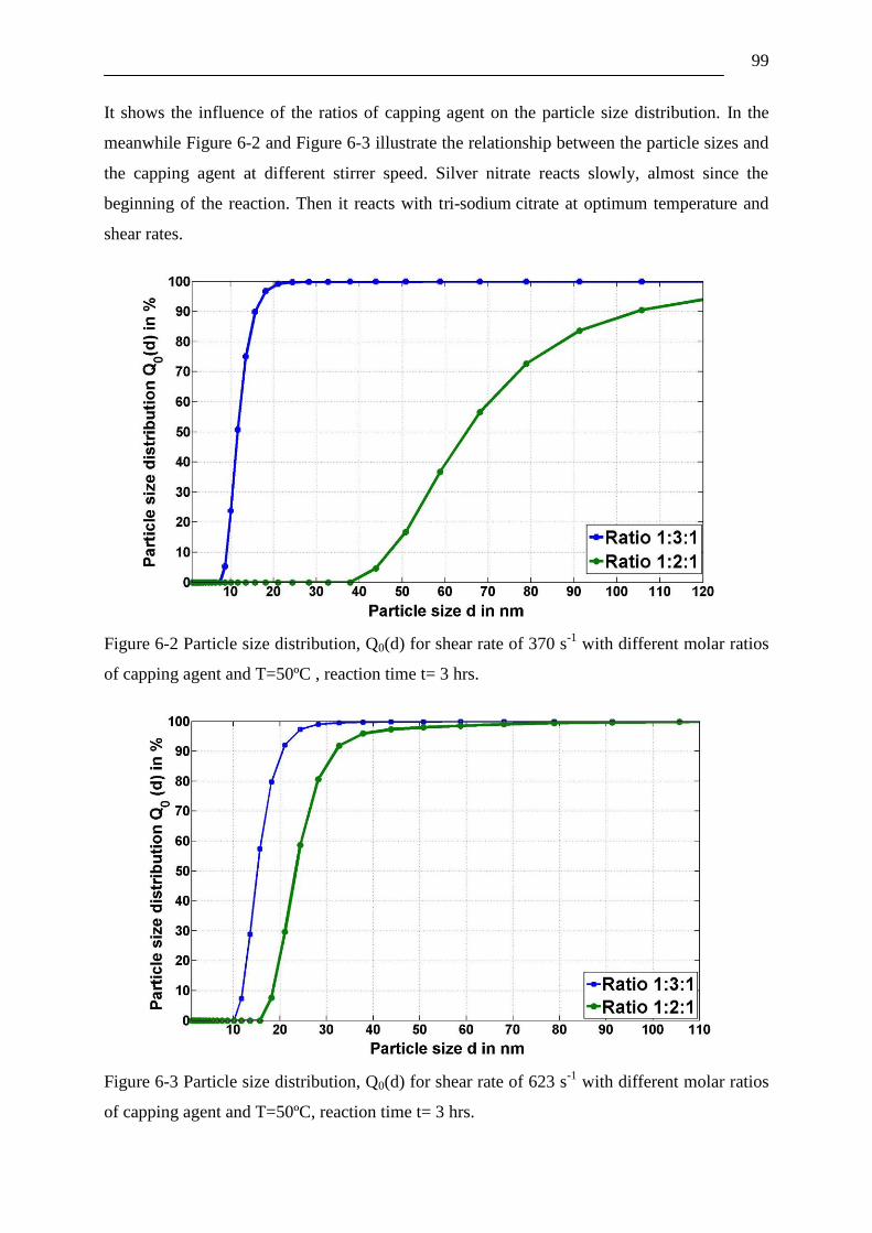
99
It shows the influence of the ratios of capping agent on the particle size distribution. In the
meanwhile Figure 6-2 and Figure 6-3 illustrate the relationship between the particle sizes and
the capping agent at different stirrer speed. Silver nitrate reacts slowly, almost since the
beginning of the reaction. Then it reacts with tri-sodium citrate at optimum temperature and
shear rates.
Figure 6-2 Particle size distribution, Q0(d) for shear rate of 370 s-1
with different molar ratios
of capping agent and T=50ºC , reaction time t= 3 hrs.
Figure 6-3 Particle size distribution, Q0(d) for shear rate of 623 s-1
with different molar ratios
of capping agent and T=50ºC, reaction time t= 3 hrs.

100
The formation of silver nanoparticles in aqueous medium proceeds rapidly and their
stabilization is primarily the result of the adsorption of negatively charged citrate ions. As
citrate plays an important role as a stabilizer; a clear yellow solution is obtained. The Table
6-1 shows that the zeta potential value asserts that a higher concentration of capping agent has
more stability on the particle charge surface than others. It makes the colloidal suspension
from the smallest particles. It is observed that particle size in the range of 14-30 nm due to
higher concentration of capping agent.
6.1.2 Effect of Reducing Agent
This study is based on the effect of reducing agent on the particle size distribution. Sodium
formaldehyde sulphoxylate (SFS) is used as mild reducing agent for reduction of silver from
Ag+ to Ag
0. The conversion of the bigger particles to smaller ones is normally done by means
of physical processes such as ball milling or mechanical grinding.
Table 6-2 shows the average particle size d50,0 of silver particles synthesized with different
molar ratios of reducing agents. Here 0.58 M silver nitrate (25ml AgNO3) with 0.45 M Tri
sodium citrate (150ml) as capping agent and 0.42 M Sodium formaldehyde sulphoxylate-SFS
(25ml) as reducing agent under different shear rates at 500 C is given.
This sulphoxylate group helps to terminate the particle growth. The use of this particle growth in
the formation of silver powder has been demonstrated.
Table 6-2 The influence of Reducing agent (Sodium Formaldehyde sulphoxylate-SFS) on
silver particles with different molar concentrations at T=50ºC and reaction time t is 3 hrs.
Number
of Variations
Variations
of
Shear rates
in s-1
Stirrer tip
speed
sV in m/s
Amount of molar
ratio AgNO3:Na-
citrate:SFS
d50,0 in
nm
Zeta Poten-
tial in mV
1 120
0.28 1:2:1 22.2 -31.5
2 1:2:0.5 59.8 -41.5
3 370 0.58 1:2:1 65.1 -30.1
4 1:2:0.5 21.1 -37.1
5 623 0.86 1:2:1 23.9 -35.2
6 1:2:0.5 18.2 -38.1

101
Figure 6-5 shows that with decrease in the particle size, also presents the molar ratio of
reducing agent increases at different shear rates. Table 6-2 also presents the particle size at
different shear rates with the variation of the reducing agent (SFS) concentration in the
solution.
Figure 6-4 Particle size distribution, Q0(d) for shear rate of 120 s-1
with different molar ratios
of reducing agent and T=50ºC , reaction time t= 3 hrs.
Figure 6-5 Particle size distribution, Q0(d) for shear rate of 370 s-1
with different molar ratios
of reducing agent and T=50ºC , reaction time t= 3 hrs.
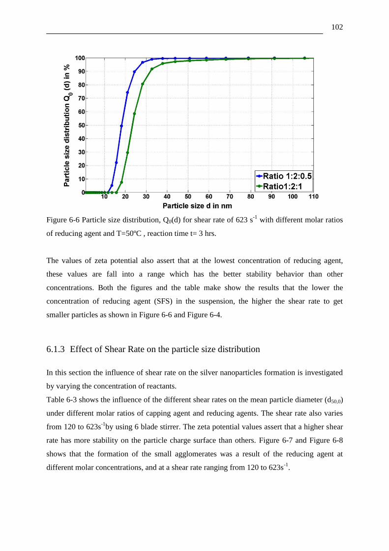
102
Figure 6-6 Particle size distribution, Q0(d) for shear rate of 623 s-1
with different molar ratios
of reducing agent and T=50ºC , reaction time t= 3 hrs.
The values of zeta potential also assert that at the lowest concentration of reducing agent,
these values are fall into a range which has the better stability behavior than other
concentrations. Both the figures and the table make show the results that the lower the
concentration of reducing agent (SFS) in the suspension, the higher the shear rate to get
smaller particles as shown in Figure 6-6 and Figure 6-4.
6.1.3 Effect of Shear Rate on the particle size distribution
In this section the influence of shear rate on the silver nanoparticles formation is investigated
by varying the concentration of reactants.
Table 6-3 shows the influence of the different shear rates on the mean particle diameter (d50,0)
under different molar ratios of capping agent and reducing agents. The shear rate also varies
from 120 to 623s-1
by using 6 blade stirrer. The zeta potential values assert that a higher shear
rate has more stability on the particle charge surface than others. Figure 6-7 and Figure 6-8
shows that the formation of the small agglomerates was a result of the reducing agent at
different molar concentrations, and at a shear rate ranging from 120 to 623s-1
.

103
Table 6-3 The influence of shear rate on silver particles with different molar concentrations at
T=50ºC
Number
of
Variations
Amount of molar ratio
AgNO3:Na-citrate:SFS
Variations of
Shear rates in
s-1
Stirrer tip
speed
sV in m/s
d50,0
in nm
Zeta Potential
in mV
1
1:2:1
120 0.28 65.1 -28.5
2 370 0.58 25.2 -38.5
3 623 0.86 22.1 -41.5
4
1:2:0.5
120 0.28 59.1 -27.6
5 370 0.58 21.1 -31.5
6 623 0.86 18.2 -37.2
Figure 6-7 Particle size distribution, Q0(d) for different shear rates with molar ratios of 1:2:1
and T=50ºC , reaction time t= 3 hrs.
As observed from the experimental results, the growth in aggregates size is faster at higher
shear rate. The formation of the bigger agglomerates occurs at a low stirrer speed from
starting process 120s-1
.It apparently means that shear rates close to the impeller are too high to
cause agglomeration. Thus, the higher shear rates, which have greater shear stress, would lead
to more collisions and also make faster disintegration process.
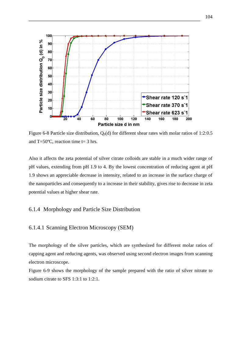
104
Figure 6-8 Particle size distribution, Q0(d) for different shear rates with molar ratios of 1:2:0.5
and T=50ºC, reaction time t= 3 hrs.
Also it affects the zeta potential of silver citrate colloids are stable in a much wider range of
pH values, extending from pH 1.9 to 4. By the lowest concentration of reducing agent at pH
1.9 shows an appreciable decrease in intensity, related to an increase in the surface charge of
the nanoparticles and consequently to a increase in their stability, gives rise to decrease in zeta
potential values at higher shear rate.
6.1.4 Morphology and Particle Size Distribution
6.1.4.1 Scanning Electron Microscopy (SEM)
The morphology of the silver particles, which are synthesized for different molar ratios of
capping agent and reducing agents, was observed using second electron images from scanning
electron microscope.
Figure 6-9 shows the morphology of the sample prepared with the ratio of silver nitrate to
sodium citrate to SFS 1:3:1 to 1:2:1.

105
A B
Figure 6-9 SEM of silver particles synthesized by addition of different molar ratio of capping
agent as A : 1:3:1 ratio and B : 1:2:1 ratio at shear rate 623 s-1
Picture A shows us the presence of small spherical primary particles with size less than 100
nm, where as in picture B particles are stuck together. Here agglomeration in the SEM images
is due to dry sample preparation.
Figure 6-10 shows that the tendency of silver particles to agglomerate is more at decreasing
shear rate 120 s-1
as compared to Figure 6-9. The difference is considered appropriate due
to the presence of hydrophilic capping around the particles which makes the dissolution
(dispersion) viable.
A B
Figure 6-10 SEM of silver particles synthesized by addition of different molar ratio of
capping agent as A : 1:3:1 ratio and B : 1:2:1 ratio at shear rate 120 s-1
The scanning electron microscopy is an analytical technique, which is appropriate for
observing particles with sizes above 100 nm. The next section shall deal with transmission
electron microscopy for particle size measurements.
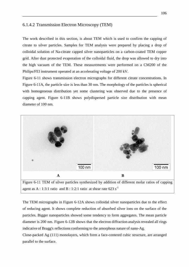
106
6.1.4.2 Transmission Electron Microscopy (TEM)
The work described in this section, is about TEM which is used to confirm the capping of
citrate to silver particles. Samples for TEM analysis were prepared by placing a drop of
colloidal solution of Na-citrate capped silver nanoparticles on a carbon-coated TEM copper
grid. After dust protected evaporation of the colloidal fluid, the drop was allowed to dry into
the high vacuum of the TEM. These measurements were performed on a CM200 of the
Philips/FEI instrument operated at an accelerating voltage of 200 kV.
Figure 6-11 shows transmission electron micrographs for different citrate concentrations. In
Figure 6-11A, the particle size is less than 30 nm. The morphology of the particles is spherical
with homogeneous distribution yet some clustering was observed due to the presence of
capping agent. Figure 6-11B shows polydispersed particle size distribution with mean
diameter of 100 nm.
A B
Figure 6-11 TEM of silver particles synthesized by addition of different molar ratios of capping
agent as A : 1:3:1 ratio and B : 1:2:1 ratio at shear rate 623 s-1
The TEM micrographs in Figure 6-12A shows colloidal silver nanoparticles due to the effect
of reducing agent. It shows complete reduction of absorbed silver ions on the surface of the
particles. Bigger nanoparticles showed some tendency to form aggregates. The mean particle
diameter is 200 nm. Figure 6-12B shows that the electron diffraction analysis revealed all rings
indicative of Bragg's reflections conforming to the amorphous nature of nano-Ag.
Close-packed Ag (111) monolayers, which form a face-centered cubic structure, are arranged
parallel to the surface.

107
A B
Figure 6-12 TEM of silver particles synthesized by addition of different molar ratios of reducing
agent as A : 1:2:0.5 ratio at shear rate 370 s-1
and B : diffraction image
0.01
0.52
10
305070
90
9899.5
0 20 40 60 80 100
0 20 40 60 80 1000
5
10
15
20
25
30
35
Pa
rtic
le s
ize
fre
qu
en
cy
dis
trib
uti
on
q0
(d
) in
nm
-1
Particle size d in nm
Cu
mu
lati
ve
Fre
qu
en
cie
s i
n %
0.01
0.52
10
305070
90
9899.5
20 40 60 80 100
20 40 60 80 1000
5
10
15
20
25
Pa
rtic
le s
ize
fre
qu
en
cy
dis
trib
uti
on
q0
(d
) in
nm
-1
Particle size d in nm
Cu
mu
lati
ve
Fre
qu
en
cie
s i
n %
A B
Figure 6-13 Cumulative frequencies (% of fraction ) and Particle size frequency distributions of
TEM images of silver particles synthesized by addition of different molar ratios of capping agent
as A : 1:3:1 ratio and B : 1:2:1 ratio at shear rate 623 s-1
The typical TEM histograms of the particle diameter are shown in Figure 6-13. Figure 6-13A
analyses particle diameter as d = 29.4 nm, d50,0 =17.6 nm, dmin = 5.8 nm, dmax = 93.6 nm.
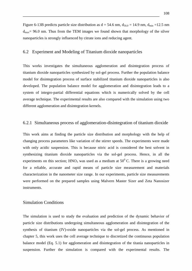
108
Figure 6-13B predicts particle size distribution as d = 54.6 nm, d50,0 = 14.9 nm, dmin =12.5 nm
dmax= 96.0 nm. Thus from the TEM images we found shown that morphology of the silver
nanoparticles is strongly influenced by citrate ions and reducing agent.
6.2 Experiment and Modeling of Titanium dioxide nanoparticles
This works investigates the simultaneous agglomeration and disintegration process of
titanium dioxide nanoparticles synthesized by sol-gel process. Further the population balance
model for disintegration process of surface stabilized titanium dioxide nanoparticles is also
developed. The population balance model for agglomeration and disintegration leads to a
system of integro-partial differential equations which is numerically solved by the cell
average technique. The experimental results are also compared with the simulation using two
different agglomeration and disintegration kernels.
6.2.1 Simultaneous process of agglomeration-disintegration of titanium dioxide
This work aims at finding the particle size distribution and morphology with the help of
changing process parameters like variation of the stirrer speeds. The experiments were made
with only acidic suspension. This is because nitric acid is considered the best solvent in
synthesizing titanium dioxide nanoparticles via the sol-gel process. Hence, in all the
experiments on this section; HNO3 was used as a medium at 500
C. There is a growing need
for a reliable, accurate and rapid means of particle size measurement and materials
characterization in the nanometer size range. In our experiments, particle size measurements
were performed on the prepared samples using Malvern Master Sizer and Zeta Nanosizer
instruments.
Simulation Conditions
The simulation is used to study the evaluation and prediction of the dynamic behavior of
particle size distributions undergoing simultaneous agglomeration and disintegration of the
synthesis of titanium (IV)-oxide nanoparticles via the sol-gel process. As mentioned in
chapter 5, this work uses the cell average technique to discretized the continuous population
balance model (Eq. 5.1) for agglomeration and disintegration of the titania nanoparticles in
suspension. Further the simulation is compared with the experimental results. The
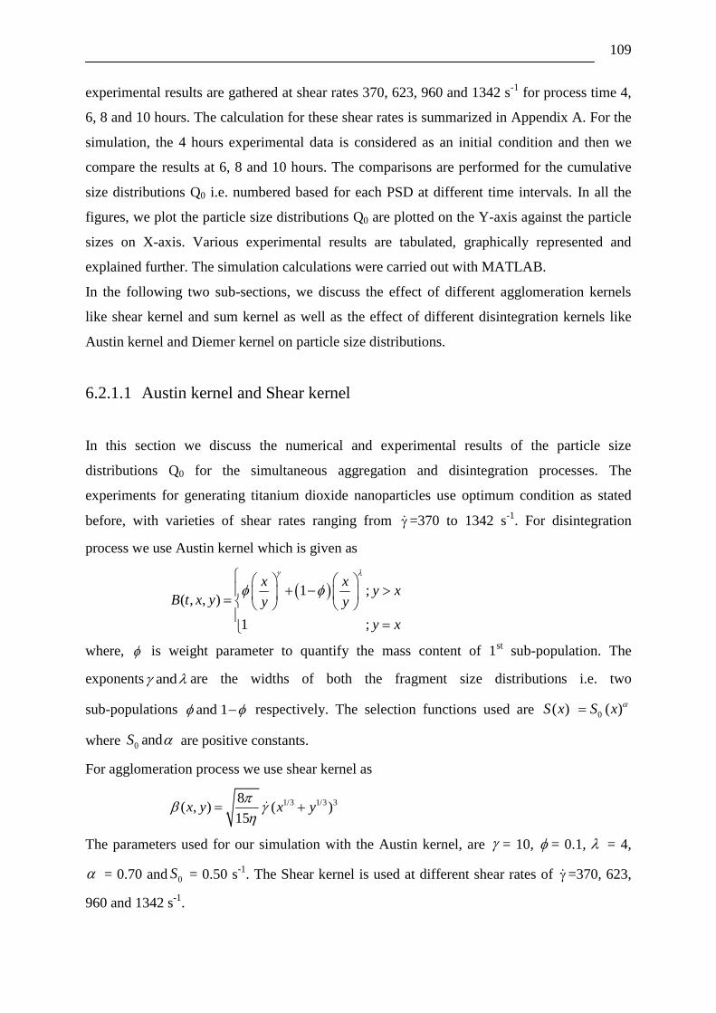
109
experimental results are gathered at shear rates 370, 623, 960 and 1342 s-1
for process time 4,
6, 8 and 10 hours. The calculation for these shear rates is summarized in Appendix A. For the
simulation, the 4 hours experimental data is considered as an initial condition and then we
compare the results at 6, 8 and 10 hours. The comparisons are performed for the cumulative
size distributions Q0 i.e. numbered based for each PSD at different time intervals. In all the
figures, we plot the particle size distributions Q0 are plotted on the Y-axis against the particle
sizes on X-axis. Various experimental results are tabulated, graphically represented and
explained further. The simulation calculations were carried out with MATLAB.
In the following two sub-sections, we discuss the effect of different agglomeration kernels
like shear kernel and sum kernel as well as the effect of different disintegration kernels like
Austin kernel and Diemer kernel on particle size distributions.
6.2.1.1 Austin kernel and Shear kernel
In this section we discuss the numerical and experimental results of the particle size
distributions Q0 for the simultaneous aggregation and disintegration processes. The
experiments for generating titanium dioxide nanoparticles use optimum condition as stated
before, with varieties of shear rates ranging from =370 to 1342 s-1
. For disintegration
process we use Austin kernel which is given as
1 ;
( , , )
1 ;
x xy x
B t x y y y
y x
where, is weight parameter to quantify the mass content of 1st sub-population. The
exponents and are the widths of both the fragment size distributions i.e. two
sub-populations and 1 respectively. The selection functions used are 0( ) ( )S x S x
where 0 andS are positive constants.
For agglomeration process we use shear kernel as
1/3 1/3 38( , ) ( )
15x y x y
The parameters used for our simulation with the Austin kernel, are = 10, = 0.1, = 4,
= 0.70 and 0S = 0.50 s-1
. The Shear kernel is used at different shear rates of =370, 623,
960 and 1342 s-1
.

110
In Figure 6-14, shear rate =370 s-1
did not show much difference in particle size distribution
compare to shear rate 623 s-1
(Figure 6-15) and 960 s
-1 (Figure 6-16) that shifted and resulted
in slightly narrower distributions than previous shear rates. This figure shows the influence of
the different shear rates on the particle size distributions under process time. Figure 6-14
expounds that predominantly the formation of the bigger agglomerates has happened at a
lower shear rate from starting process until 6 hours. Another important observation is that
increase in the redispersion time can reduce the particle sizes as expected. Moreover, during
the first 6 hrs, there is higher kinetic mechanism of agglomeration than redispersion, making
the particle size big. After 8 hrs, the redispersion dominates the process. The agglomerate
diameter becomes much smaller when compared to the previous process time.
It is seen from Figure 6-17, that particles size distribution shifted to left at applied shear rate
=1342 s-1
, indicating that very fine particles of titanium dioxide were dominated. It also
gave smaller size distribution among others. The initial stages show that polydispersed
particles were obtained due to low shear rates. In both cases monodispersed particles were
obtained after the reaction period of 10 hours. After the simulation, we observed that due to
the simultaneous agglomeration and disintegration process, shear kernel and Austin kernel
compared with the experimental results. This is shown in Figure 6-17.
Figure 6-14 Effect of shear rate 370 s-1
on PSD by Austin kernel
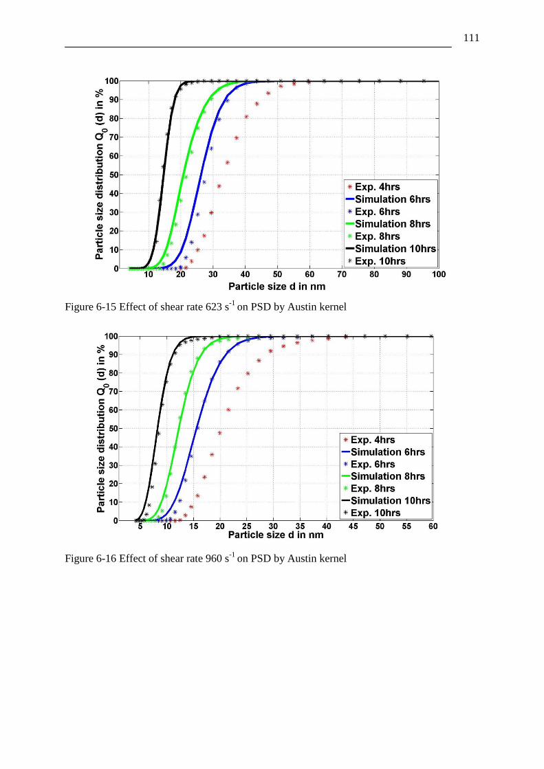
111
Figure 6-15 Effect of shear rate 623 s-1
on PSD by Austin kernel
Figure 6-16 Effect of shear rate 960 s-1
on PSD by Austin kernel

112
Figure 6-17 Effect of shear rate 1342 s-1
on PSD by Austin kernel
6.2.1.2 Diemer Kernel and Shear kernel
The numerical and experimental results of the particle size distributions Q0 for the combined
process of aggregation and disintegration are discussed. For disintegration Diemer kernel is
used which is given as,
( 1)( -2)
( -1)
( - ) ( 1)( -1) !( , )
! ( 1)( - 2) !
c c c p
pc p
p x y x c c pb x y
y c c c p
along with the selection function 0( ) ( )S x S x . The exponent p describes the number of
fragments per disintegration event and 0c determines the shape of the daughter particle
distribution. For agglomeration, the same shear kernel has been used as discussed in previous
section.
In this case, the simulation parameters are p = 2, c = 11, = 0.70 and 0S = 0.50 s-1
. It can be
seen from Figure 6-18, Figure 6-20 and Figure 6-21 that the Diemer kernel gives accurate
results with 6hours, 8 hours and 10 hours experimental results. From Figure 6-19 it is
observed that the Diemer kernel deviates slightly from the results at 6 hours and 10 hours, but
are in good agreement with 8 hours. The formation expound that predominantly the formation
of the bigger agglomerates has happened at a lower shear rate from starting process until 6
hours. Another important observation is that increasing the redispersion time can reduce the
particle sizes as expected. After 8 hours, the redispersion dominates on the process. The
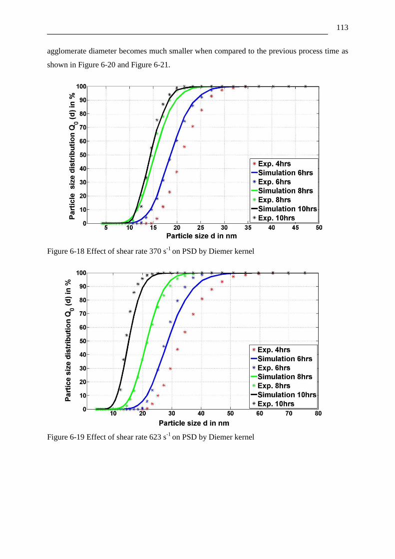
113
agglomerate diameter becomes much smaller when compared to the previous process time as
shown in Figure 6-20 and Figure 6-21.
Figure 6-18 Effect of shear rate 370 s-1
on PSD by Diemer kernel
Figure 6-19 Effect of shear rate 623 s-1
on PSD by Diemer kernel
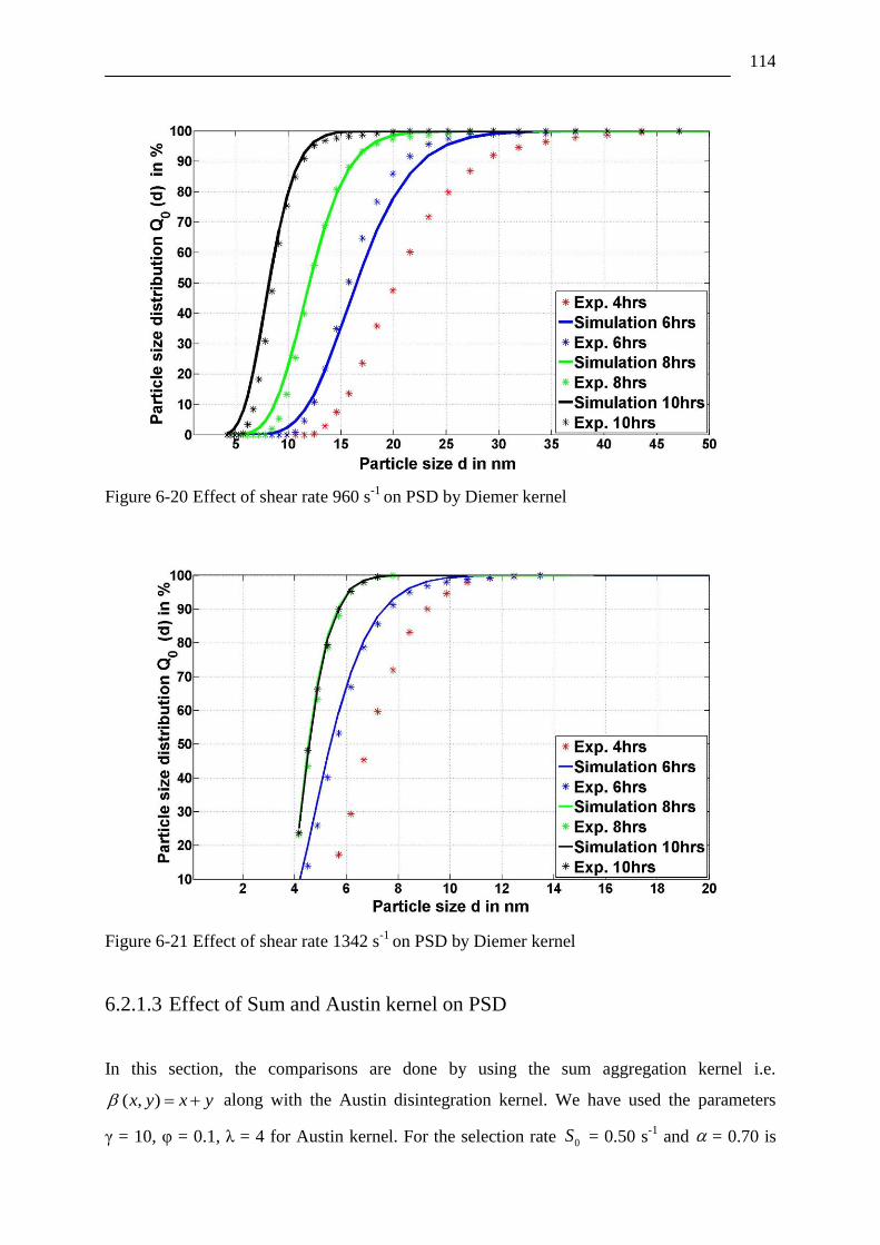
114
Figure 6-20 Effect of shear rate 960 s-1
on PSD by Diemer kernel
Figure 6-21 Effect of shear rate 1342 s-1
on PSD by Diemer kernel
6.2.1.3 Effect of Sum and Austin kernel on PSD
In this section, the comparisons are done by using the sum aggregation kernel i.e.
( , )x y x y
along with the Austin disintegration kernel. We have used the parameters
γ = 10, φ = 0.1, λ = 4 for Austin kernel. For the selection rate 0S = 0.50 s-1
and = 0.70 is
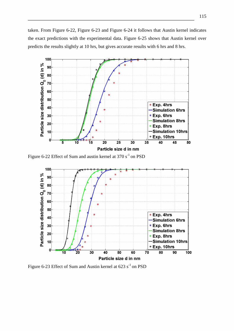
115
taken. From Figure 6-22, Figure 6-23 and Figure 6-24 it follows that Austin kernel indicates
the exact predictions with the experimental data. Figure 6-25 shows that Austin kernel over
predicts the results slightly at 10 hrs, but gives accurate results with 6 hrs and 8 hrs.
Figure 6-22 Effect of Sum and austin kernel at 370 s-1
on PSD
Figure 6-23 Effect of Sum and Austin kernel at 623 s-1
on PSD

116
Figure 6-24 Effect of Sum and Austin kernel at 960 s-1
on PSD
Figure 6-25 Effect of Sum and Austin kernel at 1342 s-1
on PSD
6.2.1.4 Effect of Sum and Diemer kernel on PSD
Here, the simulation and experimental results are compared for the sum aggregation kernel
and Diemer disintegration kernel. The simulation parameters are p = 2, c = 11 and for the
selection rate 0S = 0.50 s-1
and = 0.70 is used.
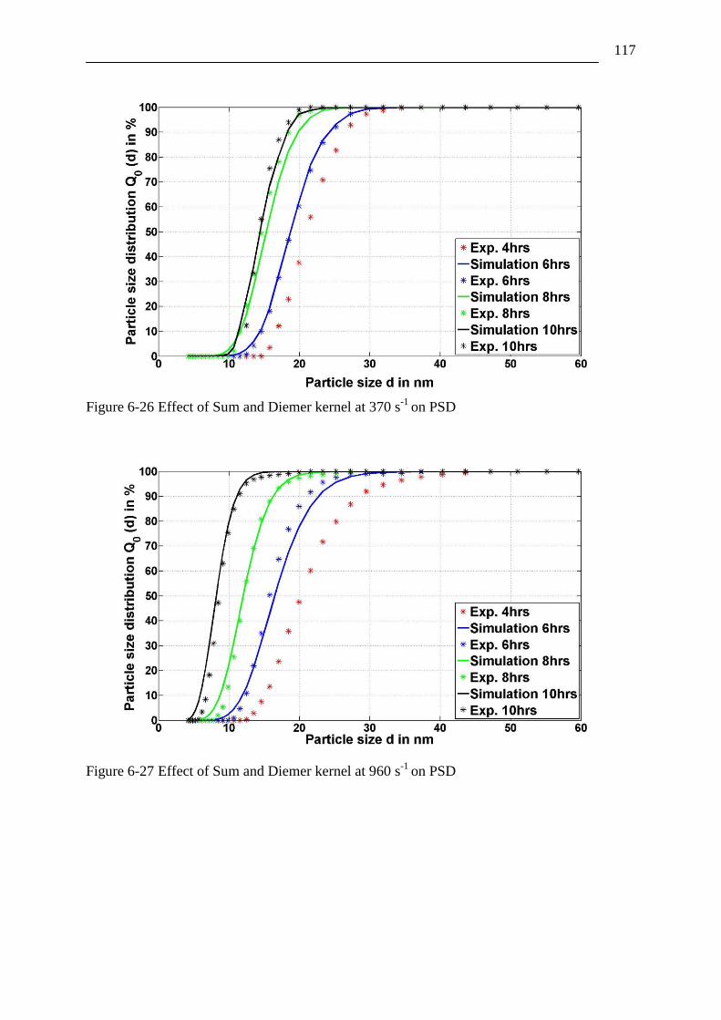
117
Figure 6-26 Effect of Sum and Diemer kernel at 370 s-1
on PSD
Figure 6-27 Effect of Sum and Diemer kernel at 960 s-1
on PSD

118
Figure 6-28 Effect of Sum and Diemer kernel at 1342 s-1
on PSD
It can be seen from Figure 6-26 and Figure 6-28 that Diemer kernel gives accurate results at
each process time interval. However from Figure 6-27 a slight under prediction of particle
sizes is observed at 6 hrs. Similarly, the Diemer kernel indicates the exact predictions with the
experimental data.
6.2.1.5 Effect of Process parameters on particle size distributions
The aim of this work is to study the influence of shear rates on the distribution of particle
sizes along with redispersion time. The applied shear rate used for experiments is =370,
623, 960, 1342, s-1
equal to 500, 750, 1000, 1250 min-1
of number of revolutions per minute
(see Table 4-2).
According to the standard condition for synthesis of titanium dioxide nanoparticles via the
sol-gel process, the large particles perceived at the initial stage of the experiment are due to
the primary particle agglomeration. Figure 6-29 shows particle size frequency distribution
q3(d) at 0, 10 and 50 minutes of redispersion time. There is a shifting of distribution to the left
as time passes, indicating that smaller particles are being produced and induced by shear rate
. The distributions continue to shift until the size of particles reaches a steady state.
Examples of graph are only taken for shear rate =1342 s-1
, which give clear view.

119
Figure 6-30 compares cumulative particle size distribution in volume basis Q3(d) from
different shear rates [ =370 s-1
; 623 s-1
; 960 s-1
; 1342 s-1
] at the initial time of redispersion
(10 minutes). The same pattern of shifting distribution is observed through whole time of
redispersion, not just at the initial time.
Figure 6-29 Particle size frequency distribution at 0, 10, and 50 minutes of redispersion time
(using =1342 s-1
)
Figure 6-30 Cumulative particle size distribution on volume basis Q3(d) in % for
different applied Shear Rates , at 10 minutes of redispersion time
Influence of shear rate on particle size distribution

120
The median is defined as d50,3 or d(0.5) in volume basis. This is the value of particle size
which divides the population exactly into two equal halves. There is 50% of the distribution
above this value and 50% below. Terms d10,3 denote that there are only less than 10% of
particle having this diameter value, while d90,3 denote that majority of population (90%) lay
before this diameter value.
Mastersizer 2000 (MS 2000) was used at initial time of experiments of total 10 hours,
measuring samples every 10 minutes. Characterization was being made by stating particles
diameter in d10,3, d50,3, d90,3.
For all characterized diameter (d10,3, d50,3, d90,3) was observed at the beginning of the
experiment due to agglomeration process. The purpose of applying shear rate is to create a
condition where the velocity gradients of fluid bring the particle close enough to collide. The
colliding session could end in agglomeration of particles or repulsion of particles depending
on the value of the repulsive interactions between particles. Agglomeration may continue to
form large, porous, and open structures agglomerates.
This Figure 6-31, Figure 6-32 and Figure 6-33 show the dependency of particle sizes upon
applied shear rates at specific time chosen (varies on each graph). Particle sizes are
characterized using d10,3, d50,3, d90,3 for applied shear rates =370, 623, 960, 1342 s-1
.
Particle Sizes during Redispersion Time, t=300 minutes
Here, Figure 6-34, Figure 6-35, Figure 6-36 and Figure 6-37 were measured using data from
Mastersizer 2000 for different shear rates =370, 623, 960, 1342 s-1
(see Table 4-2). Particle
sizes are characterized using d10,3, d50,3, d90,3 observed every 10 minutes for 300 minutes of
redispersion time. After a certain time, redispersion process becomes more significant as the
agglomerates become larger, and slows down the agglomerates growth (identified in
cascading curve), creating smaller particles. This type of agglomerates mentioned before are
more susceptible to redispersion by fluid shear of eddies turbulent when it is larger.
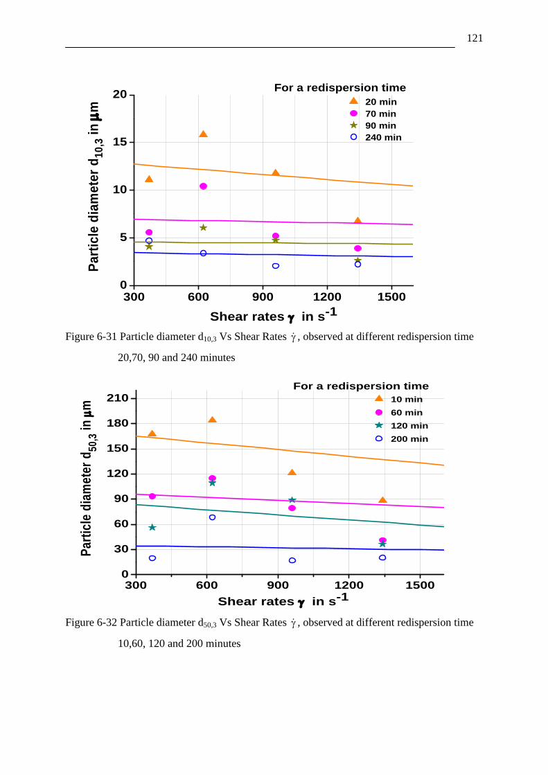
121
Figure 6-31 Particle diameter d10,3 Vs Shear Rates , observed at different redispersion time
20,70, 90 and 240 minutes
Figure 6-32 Particle diameter d50,3 Vs Shear Rates , observed at different redispersion time
10,60, 120 and 200 minutes
300 600 900 1200 15000
5
10
15
20For a redispersion time
20 min
70 min
90 min
240 min
Pa
rtic
le d
iam
ete
r d
10
,3 i
n
m
Shear rates in s-1
300 600 900 1200 15000
30
60
90
120
150
180
210For a redispersion time
10 min
60 min
120 min
200 min
Par
ticl
e d
iam
eter
d50
,3 in
m
Shear rates in s-1

122
Figure 6-33 Particle diameter d90,3 Vs Shear Rates , observed at different redispersion time
10,60, 120 and 200 minutes
Figure 6-34 Typical Decreasing Curve of Particle Sizes for 300 minutes of Redispersion time
(using =370 s-1
)
300 600 900 1200 1500
200
300
400
500
600
For a redispersion time 10 min
60 min
120 min
200 min
Pa
rtic
le d
iam
ete
r d
90
,3 i
n
m
Shear rates in s-1
0 50 100 150 200 250 300
0
100
200
300
400
500
600
Particle sizes at shear rate 370 s-1
Pa
rtic
le s
ize
s d
in
m
Redispersion time in min
d10,3
d50,3
d90,3
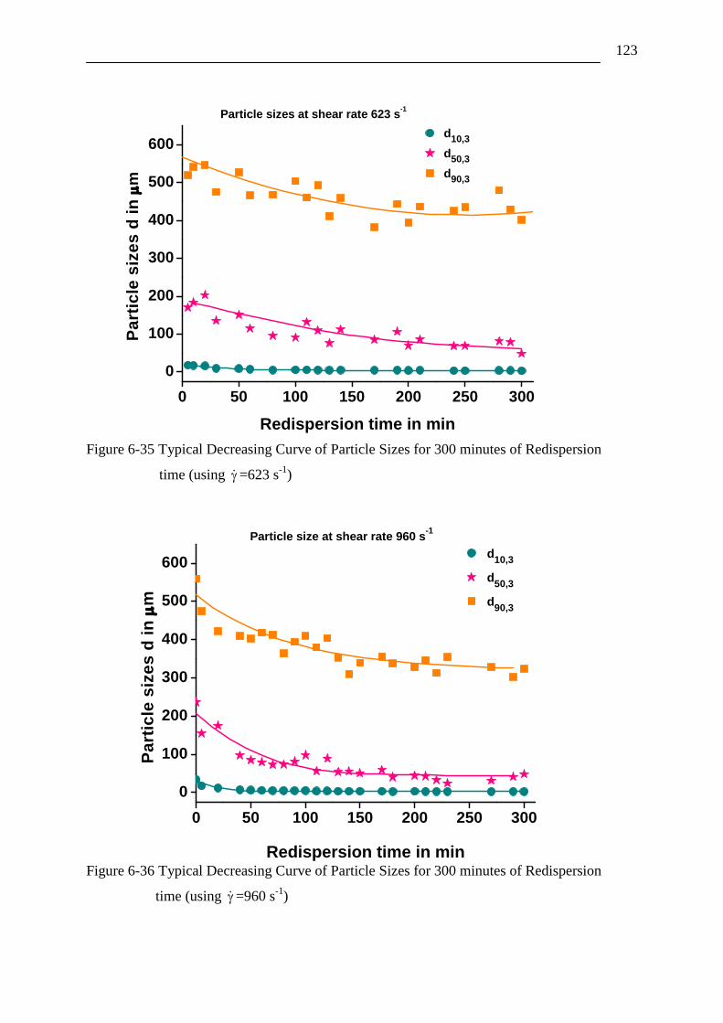
123
Figure 6-35 Typical Decreasing Curve of Particle Sizes for 300 minutes of Redispersion
time (using =623 s-1
)
Figure 6-36 Typical Decreasing Curve of Particle Sizes for 300 minutes of Redispersion
time (using =960 s-1
)
0 50 100 150 200 250 300
0
100
200
300
400
500
600
Particle size at shear rate 960 s-1
d10,3
d50,3
d90,3
Pa
rtic
le s
ize
s d
in
m
Redispersion time in min
0 50 100 150 200 250 300
0
100
200
300
400
500
600
Particle sizes at shear rate 623 s-1
d10,3
d50,3
d90,3
Pa
rtic
le s
ize
s d
in
m
Redispersion time in min

124
Figure 6-37 Typical Decreasing Curve of Particle Sizes for 300 minutes of Redispersion time
(using =1342 s-1
)
Figure 6-38 Particle size frequency distribution at 10 minutes of redispersion time by using
different kernels ( =1342 s-1
)
Figure 6-38 shows comparison of different agglomeration kernels from (Table 5-1). Besides
this, the particle size frequency is measured at a redispersion time of 10 minutes. It is
observed that shear kernel shows good comparison with initial experimental size distribution.
0 50 100 150 200 250 300
0
100
200
300
400
500
600d
10,3
d50,3
d90,3
Particle sizes at = 1342 s-1
Pa
rtic
le s
ize
s d
in
m
Redispersion time in min

125
Figure 6-39 The zeroth moment of size distribution calculated by using different
kernels ( =1342 s-1
)
In Figure 6-39, the zeroth moment is plotted using different agglomeration kernels along with
Diemer disintegration kernel (Gokhale, Kumar et al. 2008). It is observed that shear kernel
gives more number of particles as time increases. This shows that shear kernel has less
effective aggregation effect as compared to the other two kernels. It should be noted that the
total mass of the system remains conserved irrespective of the aggregation and disintegration
kernels.
Once the agglomerates are being redispersed, it can agglomerate again since the fluid velocity
will still bring particles close to each other. The same phenomena will repeat continuously
until it reaches the steady state size of agglomerates due to the balances between
agglomeration and redispersion rate. It is considered to have attained steady state when the
sizes of particles no longer changed with time.
A certain amount of energy (minimum value) must be present inside hydrodynamic fluid in
order to break agglomerates. This energy is strong enough to break the bonds between
primary particles in agglomerates. Observation of experimental and modeling data indicates
that the higher the shear rate (until a definite value of ), the narrower the distributions, and
the more they are shifted to smaller agglomerates sizes as a result of higher disintegration
rates. The optimum shear rate for generating titanium dioxide nanoparticles would be by

126
using =1342 s-1
. The next section is about disintegration process of surfactant based TiO2
nanoparticles.
6.2.2 Disintegration of Surfactant based Titanium dioxide
This work explores the effect on surface stabilization with different surfactants. The steric
stabilization of polymer and various functional groups of dispersants is also considered. The
influence of various precursor concentrations and different surfactants on the particle size
distribution is investigated. The population balance model for disintegration leads to a system
of integro-partial differential equations which is numerically solved by the cell average
technique. The experimental results are also compared with the simulation using two different
disintegration kernels.
6.2.2.1 Effects of Different Surfactants
The physical and optical properties of nano-sized particles are related strongly to their size.
For this reason, there is a growing need for a reliable, accurate and rapid means of particle
size measurement and materials characterization in the nanometer size range. Titania
nanoparticles are generated by the reduction of ionic precursors in liquid phase in the
presence of stabilizers production metal sols. Titania particles of narrow size distributions
have been synthesized in the laboratory using titanium tetra isopropoxide as precursor,
different surfactant agents notably polymers, viz. Polyethylene Glycol, Ethylene Glycol, and
Sodium Chloride.

127
Figure 6-40 Experimental sol-gel TiO2 nanoparticles in the presence of 0.372 g/ml Ethylene
Glycol and simulated evolution of PSD by the Austin kernel
The parameters used for this simulation, with the Austin kernel, are = 0.18, = 0.08,
= 10, for the selection rate 0S = 0.50 s-1
and constant = 0.33 is used.
For the other disintegration kernel we used, Diemer kernel, parameters p = 2, c = 10 and for
the selection rate 0S = 0.50 s-1
and constant = 0.70 have been considered. The 4-hour
experimental result has been held as the initial condition for the cell average scheme. The
comparisons are done for the cumulative size distributions for each PSD at different time
intervals. Various experimental results are tabulated, graphically represented and explained
further.
It can be seen from Figure 6-40 and Figure 6-41 that during the initial stages, polydispersed
particles were obtained with ethylene glycol. In both cases, monodispersed particles were
obtained after a reaction period of 10 hours. After the simulation we observed from Figure
6-40 that the Austin kernel shows good comparison with the experimental. However for the
Diemer kernel in Figure 6-41, simulation shows good behavior for PSD with experimental
data.

128
Figure 6-41 Experimental sol-gel TiO2 nanoparticles in the presence of 0.372 g/ml Ethylene
Glycol and simulated evolution of PSD by the Diemer kernel
Figure 6-42 and Figure 6-43 show the comparisons for PEG-TiO2 between the experimental
and the simulation results by using the Austin and Diemer kernels, respectively. It is found
that the simulation results, using the Austin kernel, are in excellent agreement with the
experimental results for each time interval. From Figure 6-43, it is found that Diemer kernel
gives good predictions with the experimental results. The fact that the reaction time influences
the synthesis process of titania particles is self-explanatory.
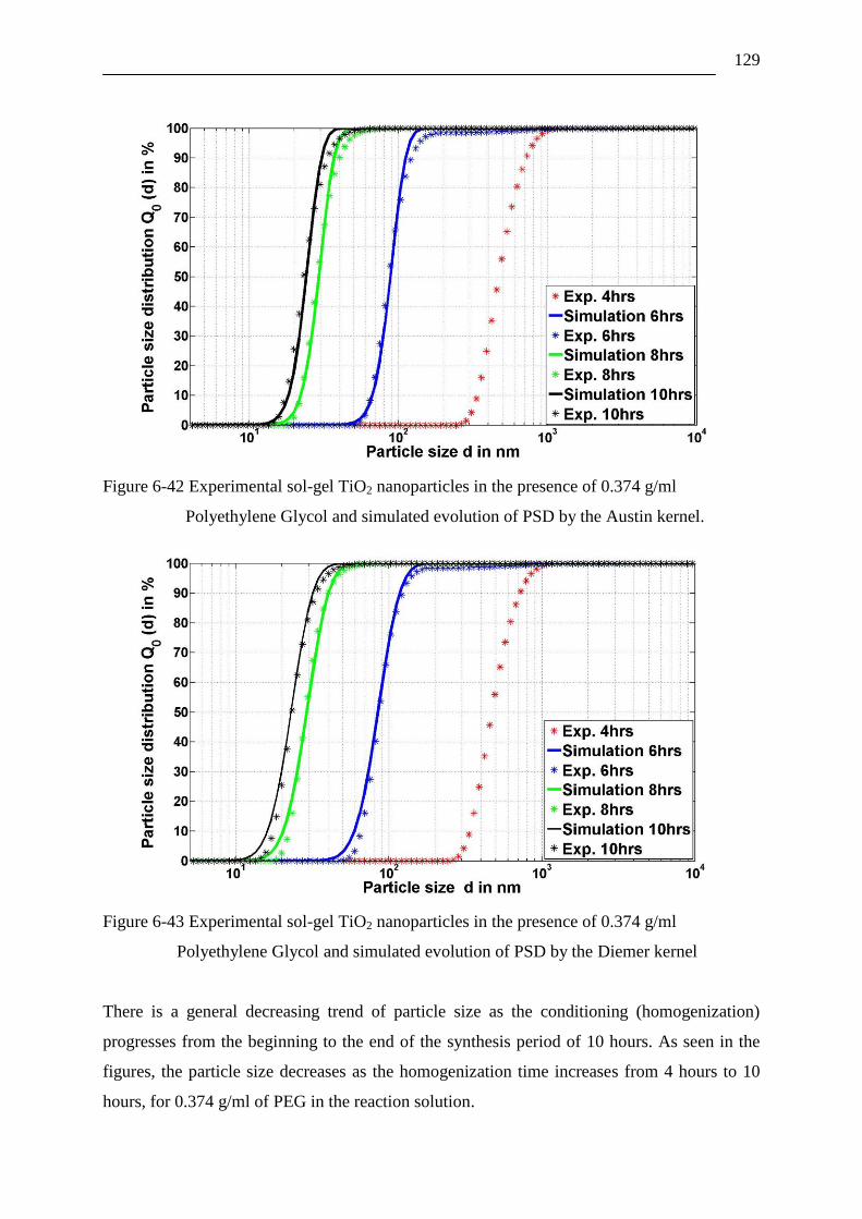
129
Figure 6-42 Experimental sol-gel TiO2 nanoparticles in the presence of 0.374 g/ml
Polyethylene Glycol and simulated evolution of PSD by the Austin kernel.
Figure 6-43 Experimental sol-gel TiO2 nanoparticles in the presence of 0.374 g/ml
Polyethylene Glycol and simulated evolution of PSD by the Diemer kernel
There is a general decreasing trend of particle size as the conditioning (homogenization)
progresses from the beginning to the end of the synthesis period of 10 hours. As seen in the
figures, the particle size decreases as the homogenization time increases from 4 hours to 10
hours, for 0.374 g/ml of PEG in the reaction solution.
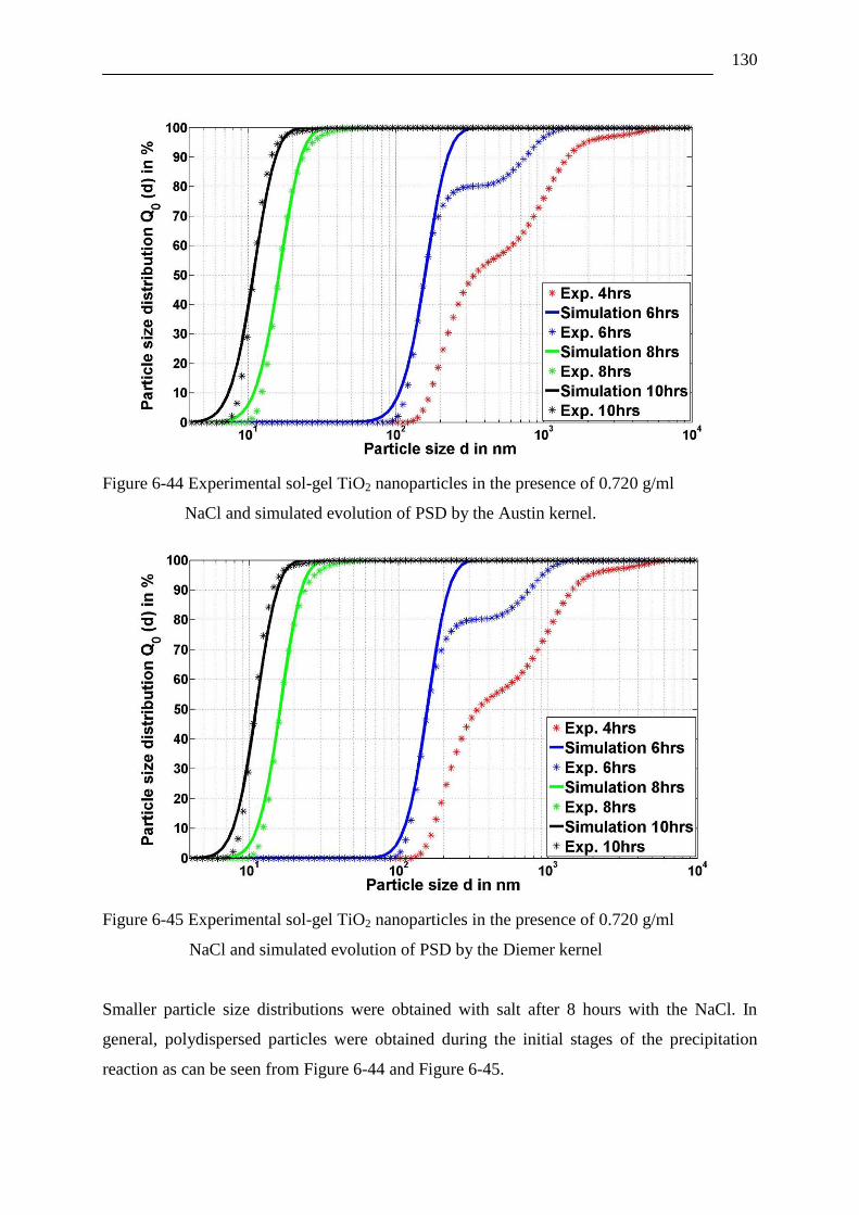
130
Figure 6-44 Experimental sol-gel TiO2 nanoparticles in the presence of 0.720 g/ml
NaCl and simulated evolution of PSD by the Austin kernel.
Figure 6-45 Experimental sol-gel TiO2 nanoparticles in the presence of 0.720 g/ml
NaCl and simulated evolution of PSD by the Diemer kernel
Smaller particle size distributions were obtained with salt after 8 hours with the NaCl. In
general, polydispersed particles were obtained during the initial stages of the precipitation
reaction as can be seen from Figure 6-44 and Figure 6-45.
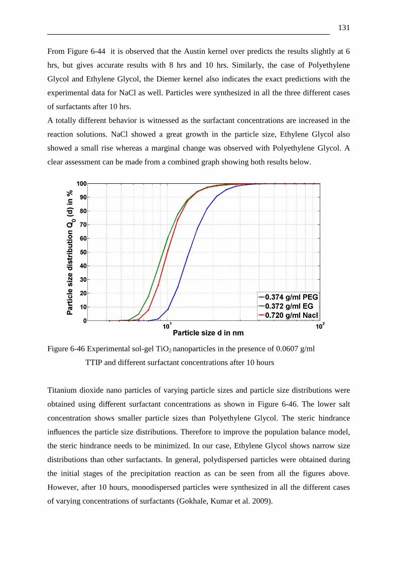
131
From Figure 6-44 it is observed that the Austin kernel over predicts the results slightly at 6
hrs, but gives accurate results with 8 hrs and 10 hrs. Similarly, the case of Polyethylene
Glycol and Ethylene Glycol, the Diemer kernel also indicates the exact predictions with the
experimental data for NaCl as well. Particles were synthesized in all the three different cases
of surfactants after 10 hrs.
A totally different behavior is witnessed as the surfactant concentrations are increased in the
reaction solutions. NaCl showed a great growth in the particle size, Ethylene Glycol also
showed a small rise whereas a marginal change was observed with Polyethylene Glycol. A
clear assessment can be made from a combined graph showing both results below.
Figure 6-46 Experimental sol-gel TiO2 nanoparticles in the presence of 0.0607 g/ml
TTIP and different surfactant concentrations after 10 hours
Titanium dioxide nano particles of varying particle sizes and particle size distributions were
obtained using different surfactant concentrations as shown in Figure 6-46. The lower salt
concentration shows smaller particle sizes than Polyethylene Glycol. The steric hindrance
influences the particle size distributions. Therefore to improve the population balance model,
the steric hindrance needs to be minimized. In our case, Ethylene Glycol shows narrow size
distributions than other surfactants. In general, polydispersed particles were obtained during
the initial stages of the precipitation reaction as can be seen from all the figures above.
However, after 10 hours, monodispersed particles were synthesized in all the different cases
of varying concentrations of surfactants (Gokhale, Kumar et al. 2009).

132
Chapter 7
Conclusions
“A man would do nothing if he tried to do it so well
that nobody would find fault with what he has done”
-John Henry Newman
“Prediction is very difficult…especially about the future”
-Niels Bohr

133
7 Conclusions and Outlook
7.1 Conclusions
his work examines the formation of nanoscale silver particles produced by chemical
double reduction method. In this, colloidal silver is obtained from silver powder. This
powder is prepared initially by the of sodium formaldehyde sulphoxylate (SFS) and
tri-sodium citrate external surfactant cum reducing agents. It is important that one can prepare
large surface capped particles in the first place and then isolated particles of smaller
dimension i.e. typically in the nano-meter regime via a colloidal stage.
TEM analysis of colloidal silver nano-particles obtained from this method showed the particle
size to be less than 30 nm. The morphology of the particles is spherical with homogeneous
distribution, despite some clustering is observed due to the presence of capping agent. It may
be due to the increase in the value of aggregation rate constant than disintegration rate
constant. The tendency of silver particles to agglomerate is more at low shear rate. The
amount of capping agent had a very desirable effect on the size of the particles. The molar
concentration of capping agent increases and the size of the nanoparticles decreases. The
amount of reducing agent has an undesirable effect on the size of nanoparticles and it is found
that the size increases with the amount of reducing agent for a given shear rate and
temperature.
Surface stabilized spherical titania particles have been synthesized in this study via the sol-gel
process. Titanium tetra isopropoxide was used as a precursor. Three different surfactants were
used for the synthesis of spherical titania particles of variable sizes. The particle size
distributions were measured by the dynamic light scattering technique. The results from
dynamic light scattering showed that the different stabilizers lead to entirely different particle
size distributions. It has been shown that size and dispersity of colloidal particles can be
controlled by appropriate choice of surfactants and polymers or salt that is added during the
synthesis.
All experiments showed that after some time particle size distribution reaches a steady state.
In the initial phase of experiments, large particles are observed, due to agglomeration process.
Disintegration of agglomerates becomes more significant as the agglomerates become larger;
it slows down the growth of agglomerates and creates smaller particles. Steady state condition
T
134
is reached as the two opposing mechanisms balance each other. Application of various shear
rates i.e., ( =370, 623, 960, 1342s-1
) to the reaction condition gives a tendency in which the
higher the shear rates, the lower is the particle size distributions. Among the entire applied
shear rates, =1342 s-1
has been determined as the optimum shear rate for generating the
smallest titanium dioxide nanoparticles.
A continuous population balance model is used for describing the simulation of the
simultaneous agglomeration and disintegration process during the sol-gel synthesis of
titanium dioxide nanoparticles. The population balance model leads to a system of
integro-partial differential equations which is numerically solved by a new numerical scheme,
the cell average technique(CAT) used in this work (Kumar 2006). The cell average technique
follows a two step strategy, one to calculate average size of the newborn nanoparticles in a
discretized cell, and the other to assign them to neighboring nodes such that the zeroth and the
first moments are properly preserved. For experimental methods, agglomeration rates are
determined by measuring the evolution of particle size distributions with time. A modeling
framework is developed by using different agglomeration kernels like Brownian, sum, and
shear kernel while for disintegration Austin and Diemer kernels are used.
The hydrodynamic factor like the shear rate has been included in the mathematical form of
solution of the kernel. Numerically derived results from a population balance model that
accounts for agglomeration and disintegration, are in reasonable agreement with experimental
observations. From the population balance model it is possible to distinguish the kernel that
best describes the experimental data based on comparison of the particle size distributions and
their moments. It is found that shear kernel and Austin kernel stands as the best fit to the
experimental data.
The experiment results of the sol-gel synthesis for titania particles are also compared with the
numerical simulation using two different disintegration kernels. The modeling and their
simulation are used are used to have a comfiration of the experiment of the sol-gel synthesis
for titania particles in addition to different surfactants.
We have observed that Austin and Diemer kernels stand in good agreement with the
experimental particle size distributions (PSD). It is also found that the Austin kernel stands as
the best fit to the experimental data as compared to the Diemer kernel. The computational
features for this method are such that, this model can be computed easily on a personal
computer.
135
7.2 Outlook
In this thesis, there is some data that shows deviation from existing theory. Based on this fact,
few suggestions and recommendations have been made to improve the result in future
research. The synthesis of Titanium dioxide nanoparticles can be done by using different
functional groups of dispersants with varying conditions. In future, simulation and modeling
of the kinetics of the reaction can be achieved with additional interaction of the colloidal
system. Also, DLVO theory can be put to use in the form of kernels for solving population
balance equations. Steric stabilization effect and Van der Waals forces can be utilized in a
form of physical kernel for different oxide nanomaterials.
There is scope for more work in the area of silver nanoparticles. Shear experiments can be
done to determine the various flow characteristics of nano powder. A model for
agglomeration, disintegration and growth of nanosized silver could be developed such that it
describes the influence of flow additives on interparticle adhesion forces. A further objective
is to apply the cell average technique for solving different physico-chemical kernels for silver
nanoparticles. Developing a large-scale method based on the model for preparation of
nanosized silver particles is a perspective goal.
While applying models to design the nano process and simulating their colloidal interactions,
the most valuable lesson to remember is that these are models that are generated by
computers. Models seldom mirror reality; in fact they often may succeed in spite of not being
completely close to reality. Models are not usually designed to simulate reality but they are
designed to produce results that agree with experiment. There are many approaches that
produce such results. These approaches may not always encompass factors operating in real
environments.
In the end however, it is experiment that is of paramount importance for building the model.
Inaccurate experimental data with uncertain error margins will undoubtedly hinder the success
of every subsequent step in model building. Therefore, generating, presenting and evaluating
accurate experimental data are the responsibilities that need to be shouldered by both nano
chemists and engineers. It is only a fruitful and synergistic alliance between the two groups
that can help overcome the complex challenges in nano process design.
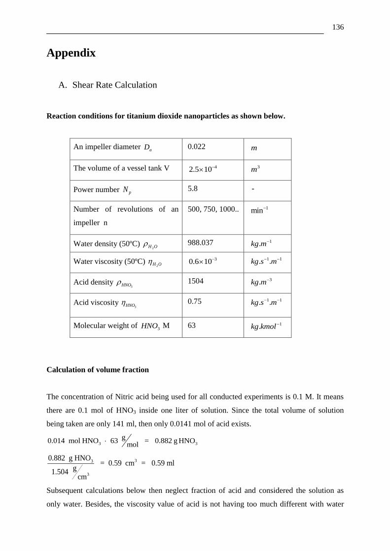
136
Appendix
A. Shear Rate Calculation
Reaction conditions for titanium dioxide nanoparticles as shown below.
An impeller diameter aD 0.022 m
The volume of a vessel tank V 42.5 10 3m
Power number pN 5.8 -
Number of revolutions of an
impeller n
500, 750, 1000.. 1min
Water density (50ºC) OH 2 988.037 1.kg m
Water viscosity (50ºC) OH 2 30.6 10 1 1. .kg s m
Acid density 3HNO 1504 3.kg m
Acid viscosity 3HNO 0.75 1 1. .kg s m
Molecular weight of 3HNO M 63 1.kg kmol
Calculation of volume fraction
The concentration of Nitric acid being used for all conducted experiments is 0.1 M. It means
there are 0.1 mol of HNO3 inside one liter of solution. Since the total volume of solution
being taken are only 141 ml, then only 0.0141 mol of acid exists.
3 3
g0.014 mol HNO 63 = 0.882 g HNO
mol
33
3
0.882 g HNO= 0.59 cm = 0.59 ml
g1.504
cm
Subsequent calculations below then neglect fraction of acid and considered the solution as
only water. Besides, the viscosity value of acid is not having too much different with water

137
and even if it is included, it would not change the viscosity of mixtures (solution)
dramatically.
Calculation of kinematic viscosity
Kinematic viscosity ( ) of solution (here, water) can be calculated as follows:
327
3
kg0.6 10
m.s m0.6 10skg
988.037m
Calculation of turbulent energy dissipation rate
Turbulent energy dissipation rate ( ) can be calculated using equation below, with six blade
impeller (Gotoh, Masuda et al. 1997).
3
-1 53 5
2p a
3-4 3
5005.8 s (0.022 m)
N n D 60 mε = = = 0.069sV 2.5 10 m
Calculation of stirrer tip speed sV
-1
s a
500 mD 3.14 s (0.022 m) = 0.58 s60
V n
Calculation of shear rate
Shear rate, can be calculated as follows (Spicer and Pratsinis 1996a)
12 2
12 3
-1
2-7
m0.069ε sγ= = =370 smυ 6 10
s
Calculation of Reynolds number Re
Reynolds number can be calculated as follows (Wang, Anderko et al. 2004)
2
a
-2 2
-7
D nRe =
500(2.2 10 )
60 = = 6719
6 10
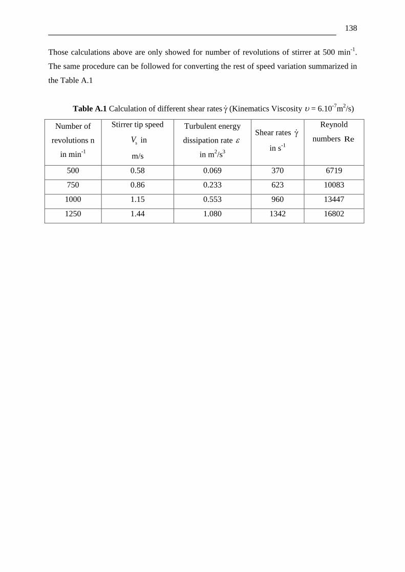
138
Those calculations above are only showed for number of revolutions of stirrer at 500 min-1
.
The same procedure can be followed for converting the rest of speed variation summarized in
the Table A.1
Table A.1 Calculation of different shear rates (Kinematics Viscosity = 6.10-7
m2/s)
Number of
revolutions n
in min-1
Stirrer tip speed
sV in
m/s
Turbulent energy
dissipation rate
in m2/s
3
Shear rates
in s-1
Reynold
numbers Re
500 0.58 0.069 370 6719
750 0.86 0.233 623 10083
1000 1.15 0.553 960 13447
1250 1.44 1.080 1342 16802
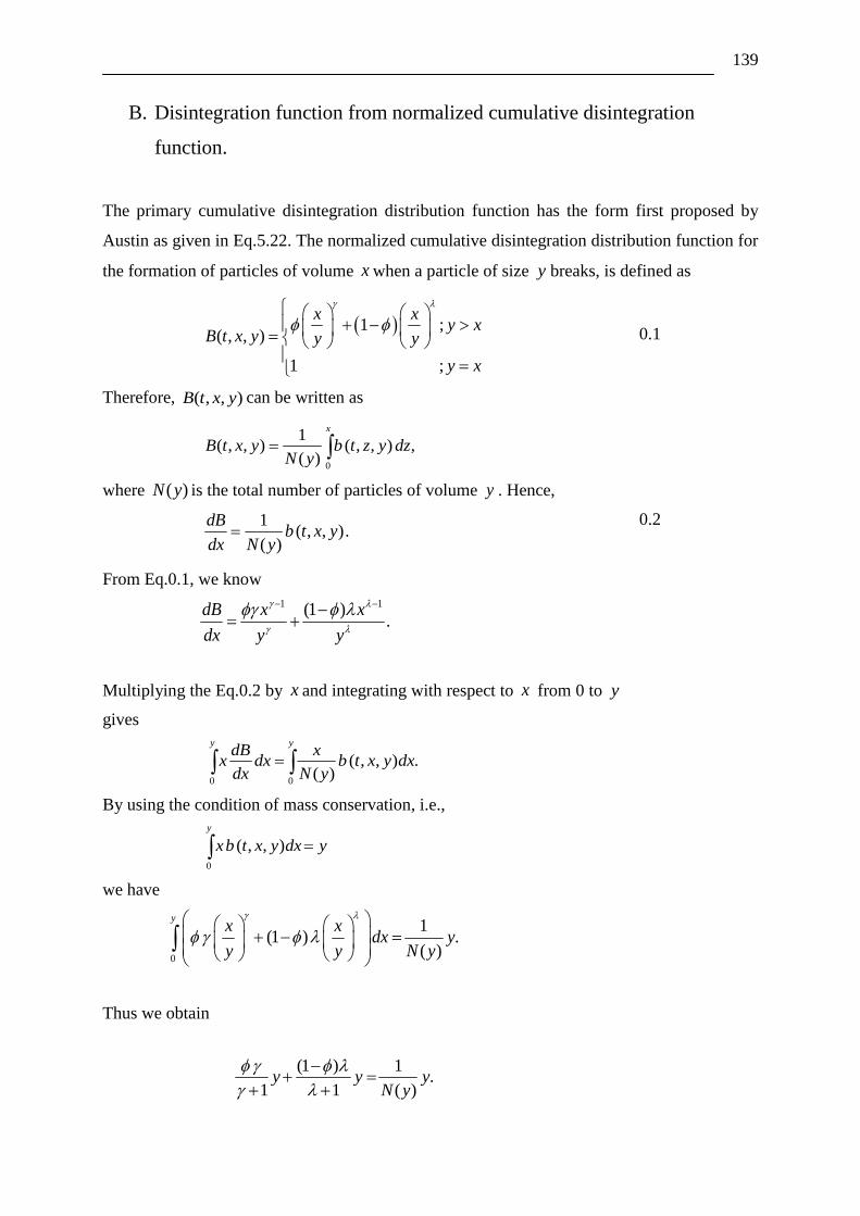
139
B. Disintegration function from normalized cumulative disintegration
function.
The primary cumulative disintegration distribution function has the form first proposed by
Austin as given in Eq.5.22. The normalized cumulative disintegration distribution function for
the formation of particles of volume x when a particle of size y breaks, is defined as
1 ;
( , , )
1 ;
x xy x
B t x y y y
y x
0.1
Therefore, ( , , )B t x y can be written as
0
1( , , ) ( , , ) ,
( )
x
B t x y b t z y dzN y
where ( )N y is the total number of particles of volume y . Hence,
1
( , , ).( )
dBb t x y
dx N y
0.2
From Eq.0.1, we know
1 1(1 ).
dB x x
dx y y
Multiplying the Eq.0.2 by x and integrating with respect to x from 0 to y
gives
0 0
( , , ) .( )
y ydB x
x dx b t x y dxdx N y
By using the condition of mass conservation, i.e.,
0
( , , )
y
xb t x y dx y
we have
0
1(1 ) .
( )
yx x
dx yy y N y
Thus we obtain
(1 ) 1
.1 1 ( )
y y yN y
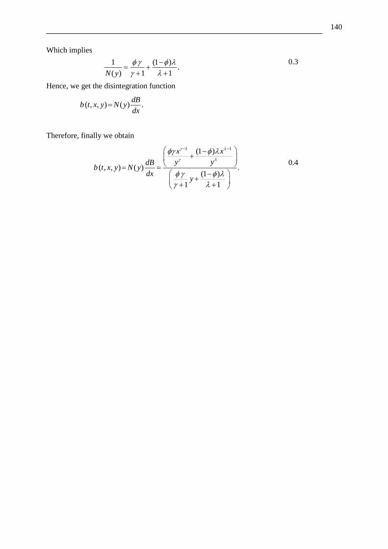
140
Which implies
1 (1 )
.( ) 1 1N y
0.3
Hence, we get the disintegration function
( , , ) ( ) .dB
b t x y N ydx
Therefore, finally we obtain
1 1(1 )
( , , ) ( ) .(1 )
1 1
x x
y ydBb t x y N y
dxy
0.4

141
“In every investigation, in every extension of knowledge, we’re
involved in action. And in every action we’re involved in choice. And
in every choice we’re involved in a kind of loss, the loss of what we
didn’t do. We find this in the simplest situations. . . . Meaning is
always obtained at the cost of leaving things out. . . . In practical
terms this means, of course, that our knowledge is always finite and
never all encompassing. . . . This makes the world of ours an open
world, a world without end. ” Robert Oppenheimer

142
Reference
Randolph, A.D. (1969). Ind.Eng.chem.Fundam 8: 58.
Adityawarman, D., A. Voigt, P. Veit and K. Sundmacher (2005). "Precipitation of BaSO4
nanoparticles in a non-ionic microemulsion: Identification of suitable control
parameters." Chemical Engineering Science 60(12): 3373-3381.
Austin, L. G. (2002). "A treatment of impact breakage of particles." Powder Technology
126(1): 85-90.
Derjaguin, B.D. (1939). Acta Physicochim USSR(10): 333.
Kaye, B.H. (1999). Characterization of powders and aerosols. Weinheim, Germany, Wiley-
VCH.
Babonneau, F., C. Sanchez and J. Livage (1988). "Spectroscopic characterization of sol-gel
processing." Journal of Non-Crystalline Solids 106(1-3): 170-173.
Bach, U., D. Lupo, P. Comte, J. E. Moser, F. Weissortel, J. Salbeck, H. Spreitzer and M.
Gratzel (1998). "Solid-state dye-sensitized mesoporous TiO2 solar cells with high
photon-to-electron conversion efficiencies." Nature 395(6702): 583-585.
Barboux-Doeuff, S. and C. Sanchez (1994). "Synthesis and characterization of titanium
oxide-based gels synthesized from acetate modified titanium butoxide precursors."
Materials Research Bulletin 29(1): 1-13.
Barrett, J. C. and J. S. Jheeta (1996). "Improving the accuracy of the moments method for
solving the aerosol general dynamic equation." Journal of Aerosol Science 27(8):
1135-1142.
Barrett, K. E. J. (1997). Dispersion polymerization in organic media. London, Wiley-
Interscience publication.
Batterham, R. J., J. S.Hall and G.Barton (1981). Proceedings, 3 rd International Symposium
on Agglomeration, Nürnberg: A136.
Bissell, E. S., H.C.Hesse, H. J. Everett and J.H.Rushton (1947). Chem.Eng.prog. 43: 649.
Boadway, J. D. (1978). "Dynamics of growth and breakage of Alum Floc in presence of fluid
shear." Journal of the Environmental Engineering Division 104: 901-991.
Brinker, C. J. and G. W. Scherer (1990). Sol Gel Science: The Physics and Chemistry of Sol
Gel Processing. New York, Academic Press.
Brown, L. O. and J. E. Hutchison (1999). "Controlled Growth of Gold Nanoparticles during
Ligand Exchange." Journal of the American Chemical Society 121(4): 882-883.
Brust, M., M. Walker, D. Bethell, D. J. Schiffrin and R. Whyman (1994). "Synthesis of thiol-
derivatised gold nanoparticles in a two-phase Liquid–Liquid system." J. Chem. Soc.
Chem. Commun.: 801-802.
Butt, H.-J., K Graf and M. kappel (2006). Physics and Chemistry of Interfaces. Weinheim,
WILEY-VCH Verlag GmbH & Co.
Buzea, C. (2007). "Nanomaterials and nanoparticles: sources and toxicity." Biointerphases
2(4): MR17-MR 71.
Calabrese, R. V., M. H. Wang, N. Zhang and J. W. Gentry (1992). "Simulation and analysis
of particle breakage phenomena." Chemical Engineering Research and Design 70(A2):
189-191.
Camp, T. R. and Stein (1943). "Velocity gradients and internal work in fluid motion." Journal
of Boston Society of Civil Engineers 30: 219-237.
Chibowski, S., M. Paszkiewicz and M. Krupa (2000). "Investigation of the influence of the
polyvinyl alcohol adsorption on the electrical properties of Al2O3-solution interface,
thickness of the adsorption layers of PVA." Powder Technology 107(3): 251-255.
Chou, K. S. and C. Y. Ren (2000). "Synthesis of nanosized silver particles by chemical
reduction method." Materials Chemistry and Physics 64(3): 241-246.
143
Cole, D. H., K. R. Shull, P. Baldo and L. Rehn (1999). "Dynamic Properties of a Model
Polymer/Metal Nanocomposite: Gold Particles in Poly(tert-butyl acrylate)."
Macromolecules 32(3): 771-779.
Collet, J.-F. (2004). "Some Modelling Issues in the Theory of Fragmentation-Coagulation
Systems " Commun. Math. Sci. 2(Supplemental Issue 1): 35-54.
Corporation, B. I. (1976). "http://www.bic.com/Zeta_Potential_overview.html."
Costas, M. E., M. Moreau and L. Vicente (1995). "Some analytical and numerical solutions
for colloidal aggregation with fragmentation." J. Phys. A Math. Gen 28: 2981–2994.
Duff, D.G., A.Baiker and P.P.Edwards (1993). "A new hydrosol of gold clusters." J Chem
Soc Chem Commun. 1: 96-98.
D.Ramkrishna (2000). Population balances. Theory and applications to particulate systems in
engineering. . New York, USA, Academic Press, New York, USA.
Danijela Vorkapic and Themis Matsoukas (1998). "Effect of Temperature and Alcohols in the
Preparation of Titania Nanoparticles from Alkoxides." Journal of the American
Ceramic Society 81(11): 2815-2820.
Danijela Vorkapic and Themis Matsoukas (2000). "Solvent Effects in the Deaggregation of
Titania Nanoparticles." Kona 18: 102-107.
Daoud, W. A. and J. H. Xin (2004). "Low Temperature Sol-Gel ProcessedPhotocatalytic
Titania coating." Journal of Sol-Gel Science and Technology(29): 25-29.
Delichatsios, M. A. and R. F. Probstein (1974). "Coagulation in turbulent flow: theory and
experiment." J. Colloid Interface Sci. 51: 394-405.
Diemer, R. B. and J. H. Olson (2002). "A moment methodology for coagulation and breakage
problems: Part 2-Moment models and distribution reconstruction." Chemical
Engineering Science 57(12): 2211-2228.
Diemer, R. B. and J. H. Olson (2002). "A moment methodology for coagulation and breakage
problems: Part 3 - generalized daughter distribution functions." Chemical Engineering
Science 57(19): 4187-4198.
Ding, A., M. J. Hounslow and C. A. Biggs (2006). "Population balance modelling of activated
sludge flocculation: Investigating the size dependence of aggregation, breakage and
collision efficiency." Chemical Engineering Science 61(1): 63-74.
Verwey, E.J.W and J. T. G. Overbeck (1948). Theory of the Stability of Lyophobic Colloids.
New York, Elservier.
Eiden-Assmann, S., J. Widoniak and G. Maret (2003). "Synthesis and Characterization of
Porous and Nonporous Monodisperse Colloidal TiO2 Particles." Chemistry of
Materials 16(1): 6-11.
Elimelech, M., J. Gregory, X. Jia and R.A.Williams (1995). Particle decomposition and
Aggregation: Measurment, Modelling and Simulation. Oxford, UK, Butterworth-
Heinemann
Everett, D. H. (1971). Symbols and Terminology for Physiocochemical Quantities and Units;
International Union of Pure andAppliedChemistry. London, Butterworths Co.
Kruis F. Einar, Arkadi Maisels and Heinz Fissan (2000). "Direct simulation Monte Carlo
method for particle coagulation and aggregation." A.I.Ch.E. Journal 46(9): 1735-1742.
Fair, G. M. and R. S. Gemmell (1964). "A mathematical model of coagulation." Journal of
Colloid Science 19(4): 360-372.
Feynman, R. P., R. B. Leighton and M.L.Sands (1995). Six Easy Pieces: Essentials of Physics
By Its Most Brilliant Teacher. Reading, Mass., Helix Books.
Filbet, F. and P. Laurencot (2004). "Numerical Simulation of the Smoluchowski Coagulation
Equation." SIAM J. Sci. Comput. 25(6): 2004-2028.
Fisher, S. M., L. H. Garcia-Rubio and E. F. Marquez (1998). Modeling of Agglomeration in
Colloidal Systems. The 3rd World Congress on Particle Technology, Brighton, UK.

144
Gokhale, Y. P., J. Kumar, W. H. and, G. Warnecke and J. Tomas (2008). Population balance
modeling for agglomeration and disintegration of nanoparticles Berlin, Springer.
Gokhale, Y. P., R. Kumar, J. Kumar, W. Hintz, G. Warnecke and J. Tomas (2009).
"Disintegration process of surface stabilized sol-gel TiO2 nanoparticles by population
balances." Chemical Engineering Science 64(24): 5302-5307.
Gotoh, K., H. Masuda and K. Higashitani (1997). Powder Technology Handbook, 2nd
edition
Revised and Expanded. New York, Marcel Dekker Inc.
Green, M. and P. OBrien (2000). "A simple one phase preparation of organically capped gold
nanocrystals " Chem. Commun.(3): 183 - 184.
Gregory, J. (1981). "Flocculation in laminar tube flow." Chemical Engineering Science
36(11): 1789-1794.
Gu, S., J. Onishi, E. Mine, Y. Kobayashi and M. Konno (2004). "Preparation of multilayered
gold-silica-polystyrene core-shell particles by seeded polymerization." Journal of
Colloid and Interface Science 279(1): 284-287.
Kihira, H. and E.Matijevic (1992). "An assessment of heterocoagulation theories." Advances
in Colloid and Interface Science 42: 1-31.
H.Klasen (2000). "A historical review of the use of silver in the treatment of burns.
II.Renewed interest for silver." Burns 26(2): 131-138.
Han, M. and D. F. Lawler (1992). "(Relative) insignificance of G in flocculation." Journal /
American Water Works Association 84(10): 79-91.
Harris, M. T. and C. H. Byers (1988). "Effect of solvent on the homogeneous precipitation of
titania by titanium ethoxide hydrolysis." Journal of Non-Crystalline Solids 103(1): 49-
64.
He, Y. (2004). "Preparation of polyaniline/nano-ZnO composites via a novel Pickering
emulsion route." Powder Technology 147(1-3): 59-63.
Hounslow, M. J. (1990). "Discretized population balance for continuous systems at steady
state." A.I.Ch.E. Journal 36(1): 106-116.
Hounslow, M. J., R. L. Ryall and V. R. Marshall (1988). "Discretized population balance for
nucleation, growth, and aggregation." A.I.Ch.E. Journal 34(11): 1821-1832.
Israelachvili, J. N. (1985). Intermolecular and Surface Forces. London,UK, Academic press.
Lister, J. D., D. J. Smit and M. J. Hounslow (1995). "Adjustable discretized population
balance for growth and aggregation." A.I.Ch.E. Journal 41(3): 591-603.
Rushton, J.H., E. W. Costich and H.J.Everett (1950). Chem.Eng.prog. 46: 395.
J.Tomas (2007). "Lecture notes of Mechanical Process Engineering,." Otto-von-Guericke
University, Magdeburg.
J.Turkevich, P.C.Stevenson and J. Hillier (1951). "A study of the nucleation and growth
processes in the synthesis of colloidal gold." Discuss.Faraday Soc 11: 55-75.
Jana, N. R., Z. L. Wang and T. Pal (2000). "Redox Catalytic Properties of Palladium
Nanoparticles: Surfactant and Electron Donorâˆ‟Acceptor Effects." Langmuir 16(6):
2457-2463.
Jean, J. H. and T. A. Ring (2002). "Nucleation and growth of monosized titania powders from
alcohol solution." Langmuir 2(2): 251-255.
Ji, M., X. Chen, C. M. Wai and J. L. Fulton (1999). "Synthesizing and Dispersing Silver
Nanoparticles in a Water-in-Supercritical Carbon Dioxide Microemulsion." Journal of
the American Chemical Society 121(11): 2631-2632.
Jiang, Z.-J., C.-Y. Liu and L.-W. Sun (2005). "Catalytic Properties of Silver Nanoparticles
Supported on Silica Spheres." The Journal of Physical Chemistry B 109(5): 1730-
1735.
Jin, R., Y. Cao, C. A. Mirkin, K. L. Kelly, G. C. Schatz and J. G. Zheng (2001).
"Photoinduced Conversion of Silver Nanospheres to Nanoprisms." Science 294(5548):
1901-1903.
145
Chou, K.S and C.Y.Ren (2000). "Synthesis of nanosized silver particles by chemical
reduction method." Mater Chem Phys 64: 241-246.
kahovec, j., r. b. fox and k. hatada (2002). "Nomenclature of regular single-strand organic
polymers (IUPAC Recommendations 2002)." Pure and Applied Chemistry; IUPAC
74(10): 1921-1956.
Kallala, M., C. Sanchez and B. Cabane (1992). "SAXS study of gelation and precipitation in
titanium-based systems." Journal of Non-Crystalline Solids 147-148: 189-193.
Keeley, E. and P. Sherrard (1992). C.P. Cavafy, Collected Poems., Princeton University
Press.
Kim, J. and T. A. Kramer (2006). "Improved orthokinetic coagulation model for fractal
colloids: Aggregation and breakup." Chemical Engineering Science 61(1): 45-53.
Kim, J. S., E. Kuk, K. N. Yu, J. H. Kim, S. J. Park, H. J. Lee, S. H. Kim, Y. K. Park, Y. H.
Park, C. Y. Hwang, Y. K. Kim, Y. S. Lee, D. H. Jeong and M. H. Cho (2007).
"Antimicrobial effects of silver nanoparticles." Nanomedicine: Nanotechnology,
Biology, and Medicine 3(1): 95-101.
Koh, P. T. L., J. R. G. Andrews and P. H. T. Uhlherr (1986). "Floc-size distribution of
scheelite treated by shear-flocculation." International Journal of Mineral Processing
17(1-2): 45-65.
Komarneni, S. (2003). "Nanophase Materials by Hydrothermal, Microwave-Hydrothermal
and Microwave-Solvothermal Methods." Current Science 85(12): 1730-1734.
Komarneni, S. (2003). "Nanophase materials by hydrothermal, microwave-hydrothermal and
microwave-solvothermal methods, ." Current Science 85(12): 1730 -1734.
Kramer, T. A. and M. M. Clark (1997). "Influence of strain-rate on coagulation kinetics."
Journal of Environmental Engineering 123(5): 444-452.
Kumar, J. (2006). Numerical approximations of population balance equations in particulate
systems. Faculty for Mathmatics. Magdeburg, Otto-von-Guericke University
Magdeburg,. PhD thesis: 241.
Kumar, J., M. Peglow, G. Warnecke and S. Heinrich (2008). "An efficient numerical
technique for solving population balance equation involving aggregation, breakage,
growth and nucleation." Powder Technology 182(1): 81-104.
Kumar, S. and D. Ramkrishna (1996). "On the solution of population balance equations by
discretization - I. A fixed pivot technique." Chemical Engineering Science 51(8):
1311-1332.
L.D.Landau (1941). Acta Physicochim USSR(14): 633.
L.W.Casson and D. F. Lawler (1990). "Flocculation in turbulent flow: measurement and
modelling of particle size distributions." J. Am. Water Works Assoc 63(8): 54-68.
Lakhwani, S. and M. N. Rahaman (1999). "Adsorption of polyvinylpyrrolidone (PVP) and its
effect on the consolidation of suspensions of nanocrystalline CeO2 particles." Journal
of Materials Science 34(16): 3909-3912.
Lawes, G. (1987). Scanning electron microscopy and X-ray microanalysis: Analytical
chemistry by open learning, John Wiley & sons.
Li, M. and S. Mann (2000). "Emergence of Morphological Complexity in BaSO4 Fibers
Synthesized in AOT Microemulsions." Langmuir 16(17): 7088-7094.
Lidia Armelao, Renzo Bertoncello and Mattia De Dominicis (1997). "Silver nanocluster
formation in silica coatings by the sol-gel route." Advanced Materials 9(9): 736-741.
Lin, Y., K. Lee and T. Matsoukas (2002). "Solution of the population balance equation using
constant-number Monte Carlo." Chemical Engineering Science 57(12): 2241-2252.
Liufu, S., H. Xiao and Y. Li (2004). "Investigation of PEG adsorption on the surface of zinc
oxide nanoparticles." Powder Technology 145(1): 20-24.
M.Elimelech, J. Gregory, X. Jia and R. Williams (1995). Particle Deposition& Aggregation:
Measurment, Modelling and Simulation. London, Butterworth Heinemann.

146
M.Wilson, K. Kannangara, G.Smith, M.Simmons and B. Raguse (2002) "Nanotechnology.
Basic Science and Emerging Technologies."
Ma, M., Y. Zhang, W. Yu, H.-y. Shen, H.-q. Zhang and N. Gu (2003). "Preparation and
characterization of magnetite nanoparticles coated by amino silane." Colloids and
Surfaces A: Physicochemical and Engineering Aspects 212(2-3): 219-226.
Mahoney, A. W. and D. Ramkrishna (2002). "Efficient solution of population balance
equations with discontinuities by finite elements." Chemical Engineering Science
57(7): 1107-1119.
Maisels, A., F. Einar Kruis and H. Fissan (2004). "Direct simulation Monte Carlo for
simultaneous nucleation, coagulation, and surface growth in dispersed systems."
Chemical Engineering Science 59(11): 2231-2239.
Marchal, P., R. David, J. P. Klein and J. Villermaux (1988). "Crystallization and precipitation
engineering--I. An efficient method for solving population balance in crystallization
with agglomeration." Chemical Engineering Science 43(1): 59-67.
Masaru Yoshinaka, Ken Hirota and Osamu Yamaguchi (1997). "Formation and Sintering of
TiO<sub>2</sub> (Anatase) Solid Solution in the System TiO<sub>2</sub>-
SiO<sub>2</sub>." Journal of the American Ceramic Society 80(10): 2749-2753.
Matijevic, E., M. Budnik and L. Meites (1977). "Preparation and mechanism of formation of
titanium dioxide hydrosols of narrow size distribution." Journal of Colloid and
Interface Science 61(2): 302-311.
McCoy, B. J. (2002). "A population balance framework for nucleation, growth, and
aggregation." Chemical Engineering Science 57(12): 2279-2285.
MicroscopyScanning(2003).
http://serc.carleton.edu/research_education/geochemsheets/techniques/SEM.html.
Motz, S., A. Mitrovic and E. D. Gilles (2002). "Comparison of numerical methods for the
simulation of dispersed phase systems." Chemical Engineering Science 57(20): 4329-
4344.
Nabavi, M., S. Doeuff, C. Sanchez and J. Livage (1990). "Chemical modification of metal
alkoxides by solvents: A way to control sol-gel chemistry." Journal of Non-Crystalline
Solids 121(1-3): 31-34.
Napper, D. H. (1983). Polymeric Stabilization of Colloidal Dispersions. New York, Academic
Press.
Nazeeruddin, M. K., A. Kay, I. Rodicio, R. Humphry-Baker, E. Mueller, P. Liska, N.
Vlachopoulos and M. Graetzel (2002). "Conversion of light to electricity by cis-
X2bis(2,2'-bipyridyl-4,4'-dicarboxylate)ruthenium(II) charge-transfer sensitizers (X =
Cl-, Br-, I-, CN-, and SCN-) on nanocrystalline titanium dioxide electrodes." Journal
of the American Chemical Society 115(14): 6382-6390.
Nicmanis, M. and M. J. Hounslow (1996). "A finite element analysis of the steady state
population balance equation for particulate systems: Aggregation and growth."
Computers & Chemical Engineering 20(Supplement 1): S261-S266.
Nikolov, Hintz, V.Jordanova and J.Tomas (2003). "Synthesis and characterisation of titanium
dioxide nanoparticles." Journal of the University of Chemical Technology and
Metallurgy XXXVIII(3): 725-734.
Nopens, I., C. A. Biggs, B. D. Clercq, R. Govoreanu, B.-M. Wilen, P. Pant and P. A.
Vanrolleghem (2002). "Modelling the activated sludge flocculation process combining
laser light diffraction particle sizing and population balance modeling (PBM)." Water
Science and Technology 45: 41-49.
Novak, Z., Å. Knez, M. Drofenik and I. Ban (2001). "Preparation of BaTiO3 powders using
supercritical CO2 drying of gels." Journal of Non-Crystalline Solids 285(1-3): 44-49.
O'Regan, B. and M. Gratzel (1991). "A low-cost, high-efficiency solar cell based on dye-
sensitized colloidal TiO2 films." Nature 353(6346): 737-740.
147
Okumura, M., S. Tsubota, M. Iwamoto and M. Haruta (1998). "Chemical Vapor Deposition
of Gold Nanoparticles on MCM-41 and Their Catalytic Activities for the Low-
temperature Oxidation of CO and of H2." Chemistry Letters 27(4): 315-316.
Olson, W. L. and W. E. Liss (1989). Process for preparing monodisperse titania spheres,
4,543,341. Patent, U. S. WO/1989/008078.
Opoku-Agyeman, K. (2008). Synthesis and surface stabilization of sol-gel TiO2 nanoparticles
by means of chemical modification with surfactants Magdeburg, Otto-von-Guericke-
University Magdeburg, . Master Thesis.
Hiemenz, P.C. (1977). Principles of Colloid and Surface Chemistry. New York, Marcel
Dekker.
Pandya, J. D. and L. A. Spielman (1982). "Floc breakage in agitated suspensions: Theory and
data processing strategy." Journal of Colloid and Interface Science 90(2): 517-531.
Parfitt, G. D. (1981). "Dispersion of Powder in Liquids: with Special Reference to Pigments."
Applied Science 1.
Park, D. G. and J. M. Burlitch (2002). "Nanoparticles of anatase by electrostatic spraying of
an alkoxide solution." Chemistry of Materials 4(3): 500-502.
Park, S. H. and S. N. Rogak (2004). "A novel fixed-sectional model for the formation and
growth of aerosol agglomerates." Journal of Aerosol Science 35(11): 1385-1404.
Parker, D. S., W. J. Kaufman and D. D.Jenkins (1972). "Floc break-up in turbulent
flocculation processes." J. Sanit. Eng. Pro. Div. Am. Soc. Civ. Eng 98 (SA1): 79-99.
Pastoriza-Santos, I. and L. M. Liz-Marzan (2002). "Synthesis of Silver Nanoprisms in DMF."
Nano Letters 2(8): 903-905.
Patil, D. P., J. R. G. Andrews and P. H. T. Uhlherr (2001). "Shear flocculation--kinetics of
floc coalescence and breakage." International Journal of Mineral Processing 61(3):
171-188.
Peng, S. J. and R. A. Williams (1993). "Control and optinisation of mineral flocculation and
transport processes using on-line particle size analysis." Minerals Engineering 6(2):
133-153.
Peterson, T. W. (1986). "Similarity solutions for the population balance equation describing
particle fragmentation." Aerosol Science and Technology 5(1): 93-101.
Philip, D. (2009). "Biosynthesis of Au, Ag and Au-Ag nanoparticles using edible mushroom
extract." Spectrochimica Acta Part A: Molecular and Biomolecular Spectroscopy
73(2): 374-381.
Pierre, A. C. (1998). Introduction to Sol-Gel Processing. Boston, Kluwer Academic
Publishers.
Pileni, M. P., T. Gulik-Krzywicki, J. Tanori, A. Filankembo and J. C. Dedieu (1998).
"Template Design of Microreactors with Colloidal Assemblies: Control the Growth of
Copper Metal Rods." Langmuir 14(26): 7359-7363.
Pookmanee, P., G. Rujijanagul, S. Ananta, R. B. Heimann and S. Phanichphant (2004).
"Effect of sintering temperature on microstructure of hydrothermally prepared bismuth
sodium titanate ceramics." Journal of the European Ceramic Society 24(2): 517-520.
Qi, L., J. Ma, H. Cheng and Z. Zhao (1996). "Preparation of BaSO4 nanoparticles in non-
ionic w/o microemulsions." Colloids and Surfaces A: Physicochemical and
Engineering Aspects 108(1): 117-126.
Raveendran, P., J. Fu and S. L. Wallen (2003). "Completely "Green" Synthesis and
Stabilization of Metal Nanoparticles." Journal of the American Chemical Society
125(46): 13940-13941.
Reist, P. C. (1993). Aerosol science and Technology. New York, McGraw-Hill Inc.
Rodriguez, J. A. and D. W. Goodman (2002). "Surface science studies of the electronic and
chemical properties of bimetallic systems." The Journal of Physical Chemistry 95(11):
4196-4206.
148
Rong, M. Z., Q. L. Ji, M. Q. Zhang and K. Friedrich (2002). "Graft polymerization of vinyl
monomers onto nanosized alumina particles." European Polymer Journal 38(8): 1573-
1582.
ROTH, J.-E. (1991). "Grenzflächeneffekte bei der Fest/Flüssig-Trennung." Chemie Ingenieur
Technik 63: 104-115.
Saffman, P. G. and J. S. Turner (1956). "On the Collision of Drops in Turbulent Clouds." J.
Fluid Mech 1: 16.
Salmon, R. and E. Matijevic (1990). Ceramics Int. 16: 157-163.
Schmid, G. (1994). Clusters and colloid. Weinheim, VCH.
Schmid., G. (1996). Applied Homogeneous Catalysis with Organometallic Compounds.
Weinheim, Wiley-VCH.
Singh, P., K. Kumari, A. Katyal, R. Kalra and R. Chandra (2009). "Synthesis and
characterization of silver and gold nanoparticles in ionic liquid." Spectrochimica Acta
Part A: Molecular and Biomolecular Spectroscopy 73(1): 218-220.
Smoluchowski, M. (1916). "Drei vortrage uber diffusion, Brownsche molekularbewegung
und koagulation vor kolloidteilchen." Physikalische Zeitschrift 17: 557-571.
Smoluchowski, M. (1917). "Versuch einer mathematischen Theorie der Koagulationskinetic
kolloider Lösungen." Z. Phys.Chem 92: 129-168.
Sonntag, R. C. and W. b. Russel (1987). J.colloid interface science 115: 378.
Spicer, P. T. and S. E. Pratsinis (1996). "Coagulation and Fragmentation: Universal Steady-
State Particle-Size Distribution." A.I.Ch.E. Journal 42(6): 1612-1620.
Spicer, P. T. and S. E. Pratsinis (1996a). "Shear-induced flocculation: The evolution of floc
structure and the shape of the size distribution at steady state." Water Research 30(5):
1049-1056.
Stabel, A., K. Eichhorst-Gerner, J. P. Rabe and A. R. Gonzalez-Elipe (1998). "Surface
Defects and Homogeneous Distribution of Silver Particles on HOPG." Langmuir
14(25): 7324-7326.
Stratton, D. M. (1994). "Coagulation algorithms with size binning." Journal of Computational
Physics 112(2): 364-369.
Summers, M., J. Eastoe and S. Davis (2002). "Formation of BaSO4 Nanoparticles in
Microemulsions with Polymerized Surfactant Shells." Langmuir 18(12): 5023-5026.
Tai, C. Y., Y. H. Wang, Y. W. Kuo, M. H. Chang and H. S. Liu (2009). "Synthesis of silver
particles below 10 nm using spinning disk reactor." Chemical Engineering Science
64(13): 3112-3119.
Thompson, P. D. (1968). proceedings International Conference Cloud Physics, Toronto: 115.
Toma, F. L., G. Bertrand, S. O. Chwa, C. Meunier, D. Klein and C. Coddet. (2006).
"Comparative study on the photocatalytic decomposition of nitrogen oxides using
TiO2 coatings prepared by conventional plasma spraying and suspension plasma
spraying. ." Surface and Coatings Technology 200((20-21)): 5855 - 5862.
U.Schubert and N. Hüsing (2000). Synthesis of Inorganic Materials. Weinheim, Wiley VCH.
Vanni, M. (2000). "Approximate population balance equations for aggregation-breakage
processes." Journal of Colloid and Interface Science 221(2): 143-160.
Verkoeijen, D., G. A. Pouw, G. M. H. Meesters and B. Scarlett (2002). "Population balances
for particulate processes--a volume approach." Chemical Engineering Science 57(12):
2287-2303.
Vimala, K., K. Samba Sivudu, Y. Murali Mohan, B. Sreedhar and K. Mohana Raju (2009).
"Controlled silver nanoparticles synthesis in semi-hydrogel networks of
poly(acrylamide) and carbohydrates: A rational methodology for antibacterial
application." Carbohydrate Polymers 75(3): 463-471.

149
Vorkapic and Matsoukas (1998). "Effect of Temperature and Alcohols in the Preparation of
Titania Nanoparticles from Alkoxides." Journal of the American Ceramic Society
81(11): 2815-2820.
W.L.McCabe, J.C. Smith and P.Harriot (2001). Unit Operations of Chemical Engineering.
New York, McGraw-Hill.
Wang, P., A. Anderko and R. D. Young (2004). "Modeling viscosity of concentrated and
mixed-solvent electrolyte systems." Fluid Phase Equilibria 226: 71-82.
Wang, W., X. Chen and S. Efrima (1999). "Silver Nanoparticles Capped by Long-Chain
Unsaturated Carboxylates." The Journal of Physical Chemistry B 103(34): 7238-7246.
White, E. T. and D. Ilievsky (1996). "The use of the population balance for modelling
metallurgical systems: Emerging separation technologies for metals II." The Minerals,
Metals and Materials Society: 91-103.
Wikipedia, S. (2009). http://en.wikipedia.org/wiki/File:Scheme_TEM_en.svg.
Wu, M., J. Long, A. Huang, Y. Luo, S. Feng and R. Xu (1999). "Microemulsion-mediated
hydrothermal synthesis and characterization of nanosize rutile and anatase particles."
Langmuir 15(26): 8822-8825.
X. Jiang, T. Herricks and Y. Xia (2003). "Monodispersed Spherical Colloids of Titania:
Synthesis, Characterization, and Crystallization." Advanced Materials 15(14): 1205-
1209.
Yaacov Almog, Shimon Reich and Moshe Levy (1982). "Monodisperse polymeric spheres in
the micron size range by a single step process." British Polymer Journal 14(4): 131-
136.
Yanagihara, N., K. Uchida, M. Wakabayashi, Y. Uetake and T. Hara (1999). "Effect of
Radical Initiators on the Size and Formation of Silver Nanoclusters in Poly(methyl
methacrylate)." Langmuir 15(9): 3038-3041.
Yang, H., K. Zhang, R. Shi, X. Li, X. Dong and Y. Yu (2006). "Sol-gel synthesis of TiO2
nanoparticles and photocatalytic degradation of methyl orange in aqueous TiO2
suspensions." Journal of Alloys and Compounds 413(1-2): 302-306.
Yang, S. and L. Gao (2005). "Preparation of titanium dioxide nanocrystallite with high
photocatalytic activities." Journal of the American Ceramic Society 88(4): 968-970.
Zetasizer-nano (2007). Zetasizer nano user manual,. http://www.malvern.com.
Zhang, Y. W., M. Tang, X. Jin, C. S. Liao and C. H. Yan (2003). "Polymeric adsorption
behavior of nanoparticulate yttria stabilized zirconia and the deposition of as-formed
suspensions on dense [alpha]-Al2O3 substrates." Solid State Sciences 5(3): 435-440.
Zhang, Y. W., M. Tang, X. Jin, C. S. Liao and C. H. Yan (2003). "Polymeric adsorption
behavior of nanoparticulate yttria stabilized zirconia and the deposition of as-formed
suspensions on dense α-Al2O3 substrates." Solid State Sciences 5(3): 435-440.
Zhu, H. Y., Y. Lan, X. P. Gao, S. P. Ringer, Z. F. Zheng, D. Y. Song and J. C. Zhao (2005).
"Phase transition between nanostructures of titanate and titanium dioxides via simple
wet-chemical reactions." Journal of the American Chemical Society 127(18): 6730-
6736.
Ziff, R. M. (1991). "New solutions to the fragmentation equation." Journal of Physics A:
Mathematical and General 24: 2821-2828.

150
Curriculum Vitae
Yashodhan Pramod Gokhale
Date of Birth: 05.10.1981 in Pune, India
Education and Experience
1999 – 2002 Bachelor of Science (B.Sc) in Chemistry, S.P. College, Pune,
University of Pune, India
2002 – 2004 Master of Science (M.Sc) in Physical Chemistry, Department of
Chemistry, University of Pune, India
2004 – 2005 Project assistant at the Center for Materials Electronic Technology
(C-MET), Nano-material‟s lab, Pune, India
2005 – 2006 Project associate at the National Chemical Laboratory, Pune, India
2006 – 2010 PhD in Chemical Process Engineering at Otto-von-Guericke
University, Magdeburg, Germany
Present Research Associate
Achievements
Brian Scarlett award for Outstanding Contribution under umbrella of Royal
Society of Chemistry (RSC) during PSA 2008 conference, UK
German Research Council (DFG) Graduiertenkolleg Scholarship
Awarded funding by CCP5 and Marie Curie Actions to attend the Summer
School workshop on : Methods in Molecular Simulation, Cardiff chemistry
workshop, UK, 2006
Publications & Conferences
Yashodhan Gokhale, Jitendra Kumar, Werner Hintz, Gerald Warnecke,
and Jürgen Tomas. Population balance modeling for agglomeration and
disintegration of nano particles, in Micro-Macro Interactions in Structured
Media and Particle Systems, p. 299–310, Springer, Berlin, June 2008, Eds.:
A. Bertram, J. Tomas
Yashodhan Gokhale, Rajesh Kumar, Jitendra Kumar, Werner Hintz,
Gerald Warnecke and Jürgen Tomas: Disintegration Process of Surface
stabilized sol-gel TiO2 nanoparticles by population balances, Chemical
Engineering Science 64 (2009), 5302-5307.
Yashodhan Gokhale, Werner Hintz and Jürgen Tomas “Modeling and
synthesis of disintegration process of surface stabilized TiO2 nanoparticles”
at Second International Conference on Polymer Processing and
Characterization (ICPPC 2010), Kerala, India, January 2010


