Download - Unbiased Bayes for Big Data

Unbiased Bayes for Big Data:Paths of Partial Posteriors
Heiko Strathmann
Gatsby Unit, University College London
Oxford ML lunch, February 25, 2015

Joint work
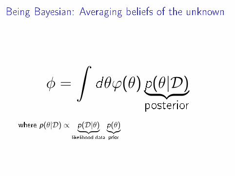
Being Bayesian: Averaging beliefs of the unknown
φ =
ˆdθϕ(θ) p(θ|D)︸ ︷︷ ︸
posterior
where p(θ|D) ∝ p(D|θ)︸ ︷︷ ︸likelihood data
p(θ)︸︷︷︸prior
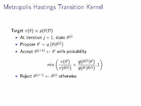
Metropolis Hastings Transition Kernel
Target π(θ) ∝ p(θ|D)
I At iteration j + 1, state θ(j)
I Propose θ′ ∼ q(θ|θ(j)
)I Accept θ(j+1) ← θ′ with probability
min
(π(θ′)
π(θ(j))× q(θ(j)|θ′)
q(θ′|θ(j)), 1
)I Reject θ(j+1) ← θ(j) otherwise.
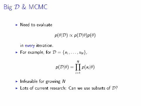
Big D & MCMC
I Need to evaluate
p(θ|D) ∝ p(D|θ)p(θ)
in every iteration.
I For example, for D = {x1, . . . , xN},
p(D|θ) =N∏i=1
p(xi |θ)
I Infeasible for growing N
I Lots of current research: Can we use subsets of D?
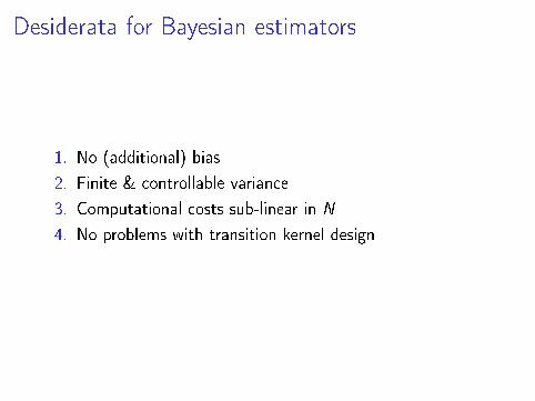
Desiderata for Bayesian estimators
1. No (additional) bias
2. Finite & controllable variance
3. Computational costs sub-linear in N
4. No problems with transition kernel design

Outline
Literature Overview
Partial Posterior Path Estimators
Experiments & Extensions
Discussion

Outline
Literature Overview
Partial Posterior Path Estimators
Experiments & Extensions
Discussion
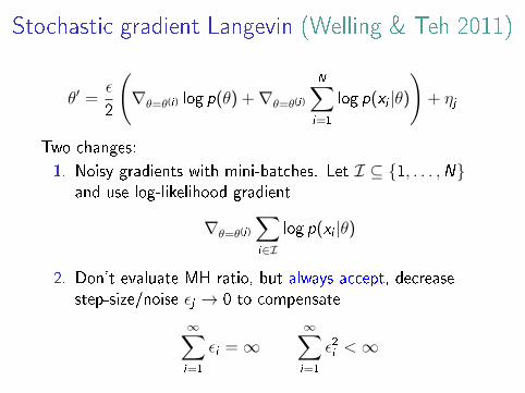
Stochastic gradient Langevin (Welling & Teh 2011)
θ′ =ε
2
(∇θ=θ(j) log p(θ) +∇θ=θ(j)
N∑i=1
log p(xi |θ)
)+ ηj
Two changes:
1. Noisy gradients with mini-batches. Let I ⊆ {1, . . . ,N}and use log-likelihood gradient
∇θ=θ(j)
∑i∈I
log p(xi |θ)
2. Don't evaluate MH ratio, but always accept, decreasestep-size/noise εj → 0 to compensate
∞∑i=1
εi =∞∞∑i=1
ε2i <∞
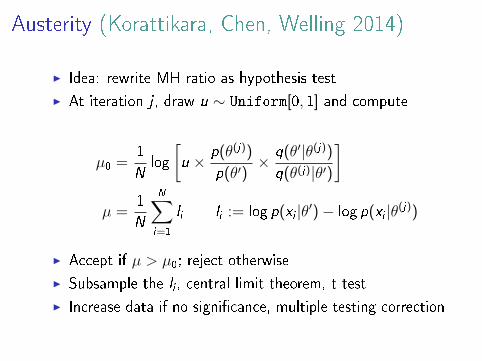
Austerity (Korattikara, Chen, Welling 2014)
I Idea: rewrite MH ratio as hypothesis test
I At iteration j , draw u ∼ Uniform[0, 1] and compute
µ0 =1
Nlog
[u × p(θ(j))
p(θ′)× q(θ′|θ(j))
q(θ(j)|θ′)
]µ =
1
N
N∑i=1
li li := log p(xi |θ′)− log p(xi |θ(j))
I Accept if µ > µ0; reject otherwise
I Subsample the li , central limit theorem, t-test
I Increase data if no signi�cance, multiple testing correction
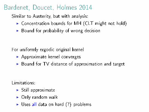
Bardenet, Doucet, Holmes 2014Similar to Austerity, but with analysis:
I Concentration bounds for MH (CLT might not hold)
I Bound for probability of wrong decision
For uniformly ergodic original kernel
I Approximate kernel converges
I Bound for TV distance of approximation and target
Limitations:
I Still approximate
I Only random walk
I Uses all data on hard (?) problems
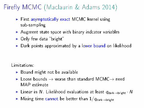
Fire�y MCMC (Maclaurin & Adams 2014)
I First asymptotically exact MCMC kernel usingsub-sampling
I Augment state space with binary indcator variables
I Only few data �bright�
I Dark points approximated by a lower bound on likelihood
Limitations:
I Bound might not be available
I Loose bounds → worse than standard MCMC→ needMAP estimate
I Linear in N. Likelihood evaluations at least qdark→bright · NI Mixing time cannot be better than 1/qdark→bright
Alternative transition kernels
Existing methods construct alternative transition kernels.(Welling & Teh 2011), (Korattikara, Chen, Welling 2014), (Bardenet, Doucet, Holmes 2014)(Maclaurin & Adams 2014), (Chen, Fox, Guestrin 2014).
They
I use mini-batches
I inject noise
I augment the state space
I make clever use of approximations
Problem: Most methods
I are biased
I have no convergence guarantees
I mix badly
Reminder: Where we came from � expectations
Ep(θ|D) {ϕ(θ)} ϕ : Θ→ R
Idea: Assuming the goal is estimation, give up on simulation.

Outline
Literature Overview
Partial Posterior Path Estimators
Experiments & Extensions
Discussion
Idea Outline
1. Construct partial posterior distributions
2. Compute partial expectations (biased)
3. Remove bias
Note:
I No simulation from p(θ|D)
I Partial posterior expectations less challenging
I Exploit standard MCMC methodology & engineering
I But not restricted to MCMC
Disclaimer
Goal is not to replace posterior sampling, but to provide a ...
I di�erent perspective when the goal is estimation
Method does not do uniformly better than MCMC, but ...
I we show cases where computational gains can be achieved
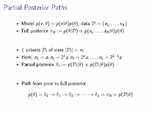
Partial Posterior Paths
I Model p(x , θ) = p(x |θ)p(θ), data D = {x1, . . . , xN}I Full posterior πN := p(θ|D) ∝ p(x1, . . . , xN |θ)p(θ)
I L subsets Dl of sizes |Dl | = nl
I Here: n1 = a, n2 = 21a, n3 = 22a, . . . , nL = 2L−1a
I Partial posterior πl := p(Dl |θ) ∝ p(Dl |θ)p(θ)
I Path from prior to full posterior
p(θ) = π0 → π1 → π2 → · · · → πL = πN = p(D|θ)
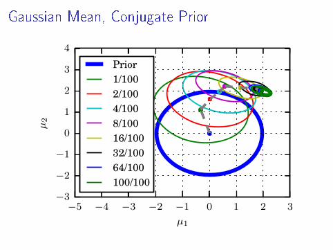
Gaussian Mean, Conjugate Prior
−5 −4 −3 −2 −1 0 1 2 3
µ1
−3
−2
−1
0
1
2
3
4µ2
Prior1/1002/1004/1008/10016/10032/10064/100100/100
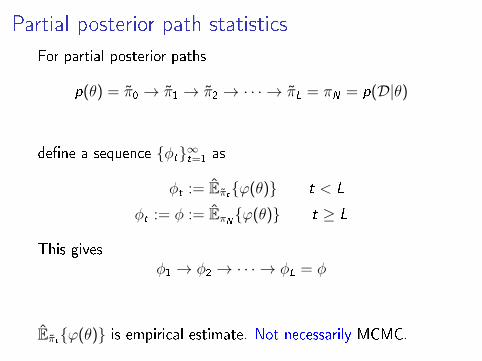
Partial posterior path statistics
For partial posterior paths
p(θ) = π0 → π1 → π2 → · · · → πL = πN = p(D|θ)
de�ne a sequence {φt}∞t=1 as
φt := Eπt{ϕ(θ)} t < L
φt := φ := EπN{ϕ(θ)} t ≥ L
This givesφ1 → φ2 → · · · → φL = φ
Eπt{ϕ(θ)} is empirical estimate. Not necessarily MCMC.
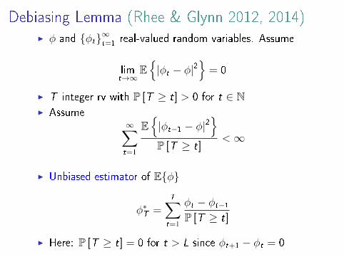
Debiasing Lemma (Rhee & Glynn 2012, 2014)I φ and {φt}∞t=1 real-valued random variables. Assume
limt→∞
E{|φt − φ|2
}= 0
I T integer rv with P [T ≥ t] > 0 for t ∈ NI Assume
∞∑t=1
E{|φt−1 − φ|2
}P [T ≥ t]
<∞
I Unbiased estimator of E{φ}
φ∗T =T∑
t=1
φt − φt−1P [T ≥ t]
I Here: P [T ≥ t] = 0 for t > L since φt+1 − φt = 0
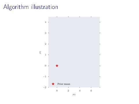
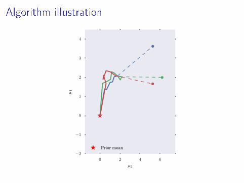
Algorithm illustration
0 2 4 6
µ2
−2
−1
0
1
2
3
4
µ1
Prior mean
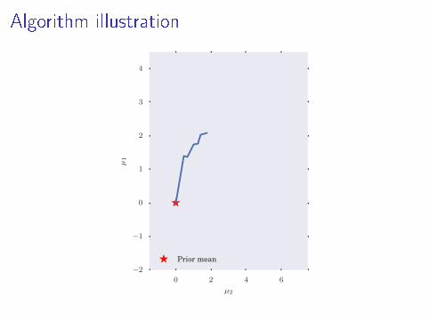
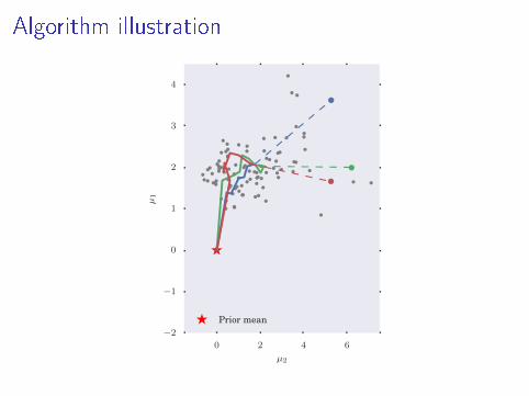
Algorithm illustration
0 2 4 6
µ2
−2
−1
0
1
2
3
4
µ1
Prior mean
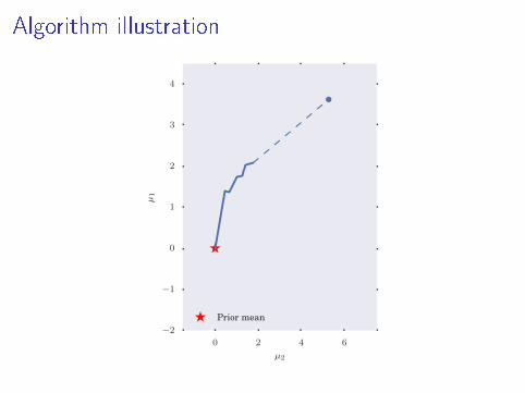
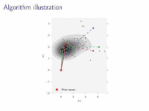
Algorithm illustration
0 2 4 6
µ2
−2
−1
0
1
2
3
4
µ1
Prior mean
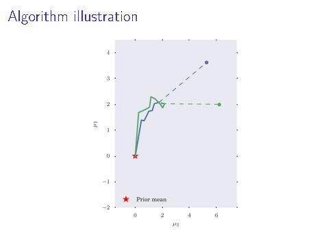
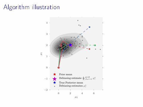
Algorithm illustration
0 2 4 6
µ2
−2
−1
0
1
2
3
4
µ1
Prior mean
Algorithm illustration
0 2 4 6
µ2
−2
−1
0
1
2
3
4
µ1
Prior mean
Algorithm illustration
0 2 4 6
µ2
−2
−1
0
1
2
3
4
µ1
Prior mean
Algorithm illustration
0 2 4 6
µ2
−2
−1
0
1
2
3
4
µ1
Prior mean
Algorithm illustration
0 2 4 6
µ2
−2
−1
0
1
2
3
4
µ1
Prior meanDebiasing estimate 1
R
∑Rr=1 ϕ
∗r
True Posterior meanDebiasing estimates ϕ∗
r
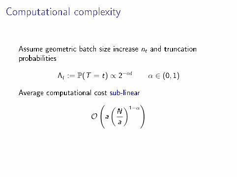
Computational complexity
Assume geometric batch size increase nt and truncationprobabilities
Λt := P(T = t) ∝ 2−αt α ∈ (0, 1)
Average computational cost sub-linear
O
(a
(N
a
)1−α)
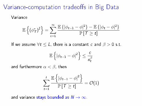
Variance-computation tradeo�s in Big Data
Variance
E{
(φ∗T )2}
=∞∑t=1
E {|φt−1 − φ|2} − E {|φt − φ|2}P [T ≥ t]
If we assume ∀t ≤ L, there is a constant c and β > 0 s.t.
E{|φt−1 − φ|2
}≤ c
nβt
and furthermore α < β, then
L∑t=1
E{|φt−1 − φ|2
}P [T ≥ t]
= O(1)
and variance stays bounded as N →∞.

Outline
Literature Overview
Partial Posterior Path Estimators
Experiments & Extensions
Discussion
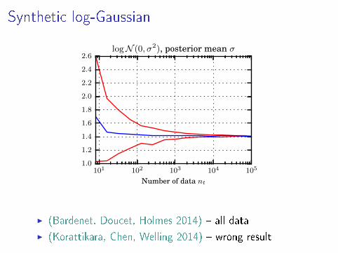
Synthetic log-Gaussian
101 102 103 104 105
Number of data nt
1.0
1.2
1.4
1.6
1.8
2.0
2.2
2.4
2.6logN (0, σ2), posterior mean σ
I (Bardenet, Doucet, Holmes 2014) � all data
I (Korattikara, Chen, Welling 2014) � wrong result
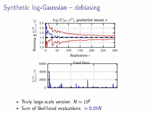
Synthetic log-Gaussian � debiasing
0 50 100 150 200 250 300
Replication r
1.0
1.2
1.4
1.6
1.8
2.0
Run
ning
1 R
∑R r=1ϕ∗ r logN (µ, σ2), posterior mean σ
0
2000
4000
6000
∑Tr
t=1nt
Used Data
I Truly large-scale version: N ≈ 108
I Sum of likelihood evaluations: ≈ 0.25N
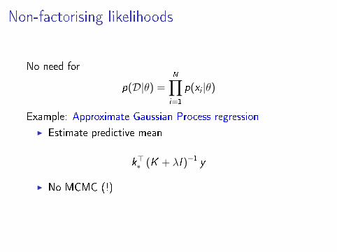
Non-factorising likelihoods
No need for
p(D|θ) =N∏i=1
p(xi |θ)
Example: Approximate Gaussian Process regression
I Estimate predictive mean
k>∗ (K + λI )−1 y
I No MCMC (!)
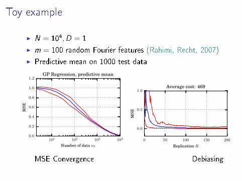
Toy example
I N = 104,D = 1
I m = 100 random Fourier features (Rahimi, Recht, 2007)
I Predictive mean on 1000 test data
101 102 103 104
Number of data nt
0.0
0.2
0.4
0.6
0.8
1.0
1.2
MSE
GP Regression, predictive mean
0 50 100 150 200
Replication R
0.0
0.5
1.0
MSE
Average cost: 469
MSE Convergence Debiasing
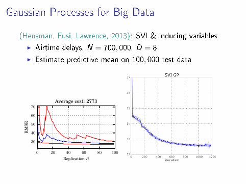
Gaussian Processes for Big Data
(Hensman, Fusi, Lawrence, 2013): SVI & inducing variables
I Airtime delays, N = 700, 000, D = 8
I Estimate predictive mean on 100, 000 test data
0 20 40 60 80 100
Replication R
30
40
50
60
70
RM
SE
Average cost: 2773

Outline
Literature Overview
Partial Posterior Path Estimators
Experiments & Extensions
Discussion
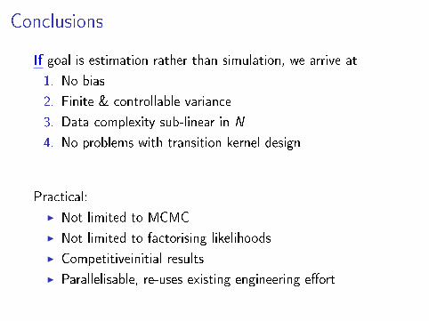
Conclusions
If goal is estimation rather than simulation, we arrive at
1. No bias
2. Finite & controllable variance
3. Data complexity sub-linear in N
4. No problems with transition kernel design
Practical:
I Not limited to MCMC
I Not limited to factorising likelihoods
I Competitiveinitial results
I Parallelisable, re-uses existing engineering e�ort
Still biased?
MCMC and �nite time
I MCMC estimator Eπt{ϕ(θ)} is not unbiasedI Could imagine two-stage process
I Apply debiasing to MC estimatorI Use to debias partial posterior path
I Need conditions on MC convergence to control variance,(Agapiou, Roberts, Vollmer, 2014)
Memory restrictions
I Partial posterior expectations need be computable
I Memory limitations cause bias
I e.g. large-scale GMRF (Lyne et al, 2014)
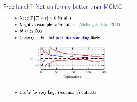
Free lunch? Not uniformly better than MCMC
I Need P [T ≥ t] > 0 for all t
I Negative example: a9a dataset (Welling & Teh, 2011)
I N ≈ 32, 000
I Converges, but full posterior sampling likely
0 50 100 150 200
Replication r
−4
−2
0
2
β1
I Useful for very large (redundant) datasets

Xi'an's og, Feb 2015
Discussion of M. Betancourt's note on HMC and subsampling.
�...the information provided by the whole data is only availablewhen looking at the whole data.�
See http://goo.gl/bFQvd6

Thank you
Questions?


