Lecture – 16

Review of Numerical Methods

Dr. Radhakant PadhiAsst. Professor

Dept. of Aerospace EngineeringIndian Institute of Science - Bangalore

ADVANCED CONTROL SYSTEM DESIGN Dr. Radhakant Padhi, AE Dept., IISc-Bangalore

2

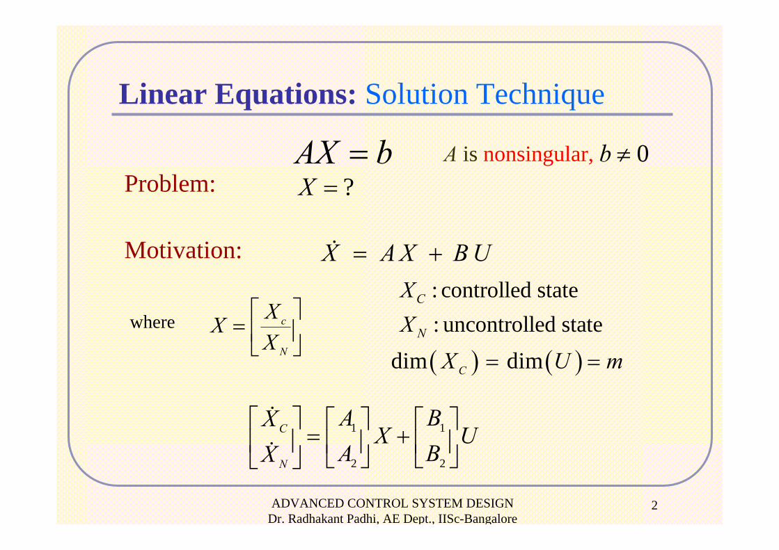
Problem:AX b=

where

X A X B U= +: controlled state: uncontrolled state

C

N

XX

( ) ( )dim dimCX U m= =

Linear Equations: Solution Technique

?X =0b ≠A is nonsingular,

Motivation:

c

N

XXX

⎡ ⎤= ⎢ ⎥

⎣ ⎦

1 1

2 2

C

N

A BXX U

A BX⎡ ⎤ ⎡ ⎤ ⎡ ⎤

= +⎢ ⎥ ⎢ ⎥ ⎢ ⎥⎣ ⎦ ⎣ ⎦⎣ ⎦

ADVANCED CONTROL SYSTEM DESIGN Dr. Radhakant Padhi, AE Dept., IISc-Bangalore

3

1 1cX A X B U= +

This will be the controller necessary to maintain at steady state

cX0

Motivation: Continued

( )11 1U B A X−= −

Which gives

Note: B1 is square

ADVANCED CONTROL SYSTEM DESIGN Dr. Radhakant Padhi, AE Dept., IISc-Bangalore

4

Solution Technique: Direct Inversion of A

Computation of Involves too many computations, roughly number of operations (very inefficient for large n).

This approach also suffers from the problem of sensitivity (ill-conditioning) ,when

Round off errors may lead to large inaccuracies

2 !n n×

1−A

0A →

1X A b−=

ADVANCED CONTROL SYSTEM DESIGN Dr. Radhakant Padhi, AE Dept., IISc-Bangalore

5

Solution Technique: Gauss Elimination

⎥⎥⎥

⎦

⎤

⎢⎢⎢

⎣

⎡=

⎥⎥⎥

⎦

⎤

⎢⎢⎢

⎣

⎡

⎥⎥⎥

⎦

⎤

⎢⎢⎢

⎣

⎡

421

110121012

3

2

1

XXX

⎥⎥⎥

⎦

⎤

⎢⎢⎢

⎣

⎡=

⎥⎥⎥

⎦

⎤

⎢⎢⎢

⎣

⎡

⎥⎥⎥

⎦

⎤

⎢⎢⎢

⎣

⎡

423

1

1101230012

3

2

1

xxx

Example:

Solution Steps:

Step-I: Multiply row-1 with -1/2 and add to the row-2. row-3 keep unchanged, since a31=0.

o Do row operations to reduce the A matrix to a upper triangular form

o Solve the variable from down to top

ADVANCED CONTROL SYSTEM DESIGN Dr. Radhakant Padhi, AE Dept., IISc-Bangalore

6

Step-II: Multiply row-2 with -2/3 and add to row-3

⎥⎥⎥

⎦

⎤

⎢⎢⎢

⎣

⎡=

⎥⎥⎥

⎦

⎤

⎢⎢⎢

⎣

⎡

⎥⎥⎥

⎦

⎤

⎢⎢⎢

⎣

⎡

323

1

31001230012

3

2

1

xxx

1

2

3

35

9

xxx

⎡ ⎤ ⎡ ⎤⎢ ⎥ ⎢ ⎥= −⎢ ⎥ ⎢ ⎥⎢ ⎥ ⎢ ⎥⎣ ⎦ ⎣ ⎦

Final Solution

Upper Triangle Matrix

Solution Technique: Gauss Elimination

ADVANCED CONTROL SYSTEM DESIGN Dr. Radhakant Padhi, AE Dept., IISc-Bangalore

7

Gauss Eliminationo The total number of operations needed is

which is far lesser than computing (which requires operations )

o The Gauss elimination method will encounter potential problems when the pivot elements i.e.. diagonal elements become zero, or very close to zero at any stage of elimination.

o In such cases the order of equations can be changed by exchanging rows and the procedure can be continued

( ) 32 / 3 n

( )A

AadjA =−1 2 !n n×

ADVANCED CONTROL SYSTEM DESIGN Dr. Radhakant Padhi, AE Dept., IISc-Bangalore

8

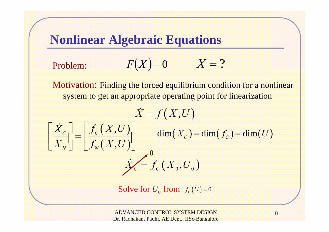
Nonlinear Algebraic Equations

Motivation: Finding the forced equilibrium condition for a nonlinear system to get an appropriate operating point for linearization

( ) 0=XF ?X =

( ),X f X U=( )( )

,,

CC

N N

f X UXX f X U

⎡ ⎤⎡ ⎤= ⎢ ⎥⎢ ⎥

⎣ ⎦ ⎣ ⎦

( )0 0,C CX f X U=

Solve for 0U from ( ) 0Cf U =

Problem:

( ) ( ) ( )dim dim dimC CX f U= =

0

ADVANCED CONTROL SYSTEM DESIGN Dr. Radhakant Padhi, AE Dept., IISc-Bangalore

9

Newton-Raphson Method: Scalar Case

( ) ( )

( )

1

( ) 0Using Taylor series expansion

( )

( )( )

From the above equation with an initial guesswe can iteratively solve for

k

k

k k k kx

k kx

kk k

k

f x

dff x x f x x higher order termsdx

df x f xdx

f xx xf x+

=

⎡ ⎤+ Δ ≈ + Δ + +⎢ ⎥⎣ ⎦

⎡ ⎤ Δ = −⎢ ⎥⎣ ⎦

= −′

with x x tolerenceΔ <

0

ADVANCED CONTROL SYSTEM DESIGN Dr. Radhakant Padhi, AE Dept., IISc-Bangalore

10

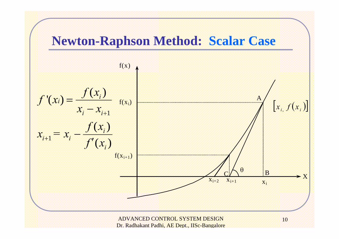
Newton-Raphson Method: Scalar Case

A

f(x)

f(xi)

f(xi+1)

xi+2 xi+1 xi X

θ

( )[ ]ii xfx ,

B C

1

1

( )'( )

( )( )

ii

i i

ii i

i

f xf xx x

f xx = x f x

+

+

=−

−′

ADVANCED CONTROL SYSTEM DESIGN Dr. Radhakant Padhi, AE Dept., IISc-Bangalore

11

( ) ( )

kA

k k k kk

FF X X F X XX

∂⎡ ⎤+ Δ ≈ + Δ⎢ ⎥∂⎣ ⎦

( )k k kA X F XΔ = −

( )1 k k kX A F X−Δ = −Solve for

Update 1k k kX X X+ = + Δ

Newton-Raphson Method: Multi Variable Case

( ) 0F X =

ADVANCED CONTROL SYSTEM DESIGN Dr. Radhakant Padhi, AE Dept., IISc-Bangalore

12

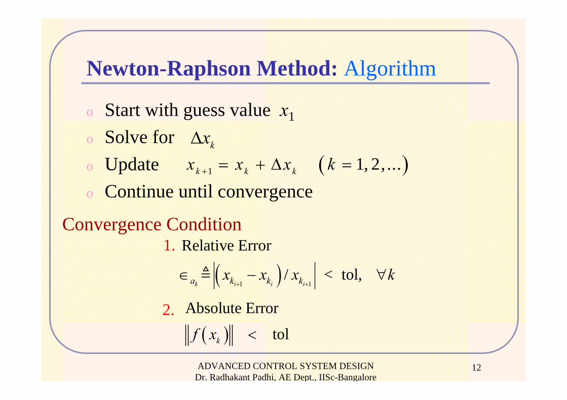
o Start with guess value x1

o Solve for o Updateo Continue until convergence

kxΔ( )1 1, 2, ...k k kx x x k+ = + Δ =

Newton-Raphson Method: Algorithm

Convergence Condition

( )Absolute Error

tolkf x <

1.

2.

( )1 1

Relative Error

/ < tol,k i i ia k k kx x x k

+ +∈ − ∀

ADVANCED CONTROL SYSTEM DESIGN Dr. Radhakant Padhi, AE Dept., IISc-Bangalore

13

Example: N-R Method

( )( )

( )( )

( )( )

3 2 4

20

40

1 0 30

41

2 11

Find a root of the following equation0 165 3 993x10 0

3 0 33 . Let 0.02. Then

3.413x100.02 0.08320 ' 5.4x10

1.670x100.083206.

f x x . x + .

f x x . x x

f xx x

f x

f xx x

f x

−

−

−

−

= − =

′ = − =

= − = − =−

−= − = −

′ −

Question :

Solution :

( )( )

3

52

3 2 32

0.05824689x10

3.717x100.05284 0.06235 ' 9.043x10

f xx x

f x

−

−

−

=

= − = − =−

ADVANCED CONTROL SYSTEM DESIGN Dr. Radhakant Padhi, AE Dept., IISc-Bangalore

14

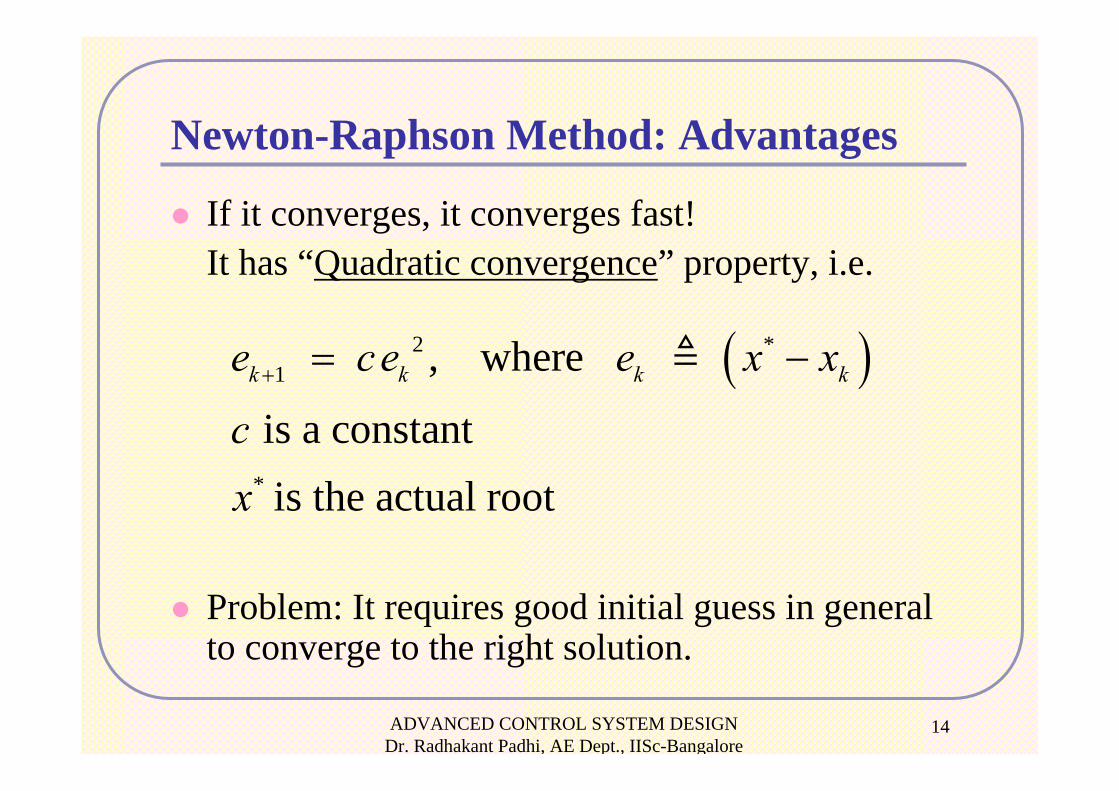
Newton-Raphson Method: Advantages

If it converges, it converges fast!It has “Quadratic convergence” property, i.e.

Problem: It requires good initial guess in general to converge to the right solution.

( )2 *1

*

, where

is a constantis the actual root

k k k ke ce e x x

cx

+ = −

ADVANCED CONTROL SYSTEM DESIGN Dr. Radhakant Padhi, AE Dept., IISc-Bangalore

15

Newton-Raphson Method: Limitations

Non-convergence at Inflection points

Inflection point x=1

For a function f(x) the points where the concavity changes from up-to-down or down-to-up are called inflection points.

( ) ( ) 01 3 =−= xxf

ADVANCED CONTROL SYSTEM DESIGN Dr. Radhakant Padhi, AE Dept., IISc-Bangalore

16

Newton-Raphson Method: LimitationsRoot Jumping

Cases where f (x) is oscillating and has a number of roots

Initial Guess near to one root may produce another root

Example:( ) sin( ) 0f x x= =

Produced root x=0

ADVANCED CONTROL SYSTEM DESIGN Dr. Radhakant Padhi, AE Dept., IISc-Bangalore

17

Newton-Raphson Method: LimitationsOscillations around local minima or maximaResults may oscillate about the local maximum or minimum without converging on a root but converging on the local maximum or minimum. Eventually, it may lead to division to a number close to zero and may diverge.

2( ) 2f x x= +

f(x) has no real roots

ADVANCED CONTROL SYSTEM DESIGN Dr. Radhakant Padhi, AE Dept., IISc-Bangalore

18

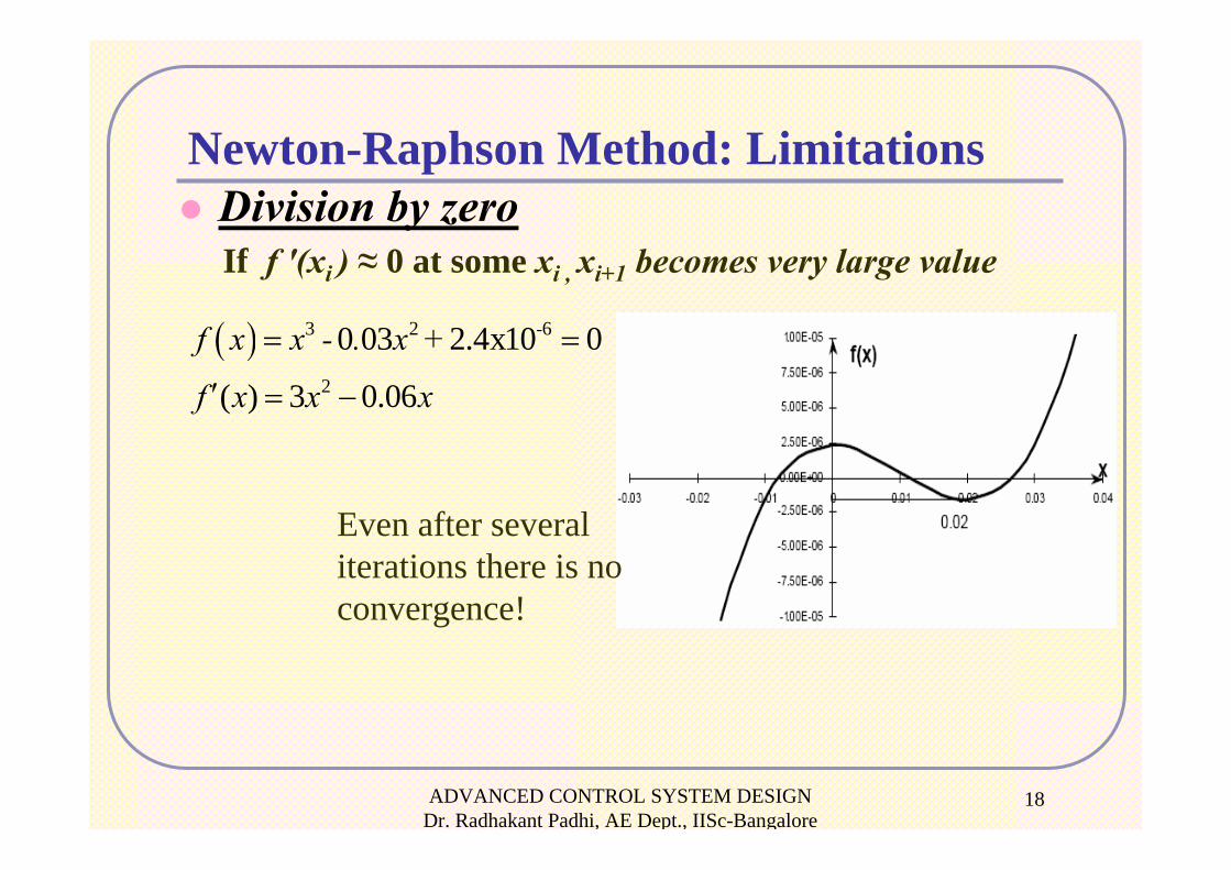
Newton-Raphson Method: LimitationsDivision by zero

( ) 3 2 6

2

0 03 2.4x10 0

( ) 3 0.06

-f x x - . x +

f x x x

= =

′ = −

If f '(xi ) ≈ 0 at some xi , xi+1 becomes very large value

Even after several iterations there is no convergence!

ADVANCED CONTROL SYSTEM DESIGN Dr. Radhakant Padhi, AE Dept., IISc-Bangalore

19

N-R Method Drawbacks

f'(x*) is unboundedIf the derivative of f(x) is unbounded at theroot then Newton-Raphson method will not converge.

Exercise: Verify for f(x)=√x

ADVANCED CONTROL SYSTEM DESIGN Dr. Radhakant Padhi, AE Dept., IISc-Bangalore

20

Numerical Differentiation

Centraldifference

Backward difference

Forward difference

ErrorNumerical Approximation

DefinitionTechnique Name

( )2O xΔ

( )O xΔ( ) ( )0 0f x x f xx

+ Δ −Δ

( ) ( )0 0f x f x xx

− − ΔΔ

( ) ( )0 0

2f x x f x x

x+Δ − −Δ

Δ

( ) ( )0

limx

f x x f xxΔ →

+Δ −⎡ ⎤⎢ ⎥Δ⎣ ⎦

( ) ( )0

limx

f x f x xxΔ →

− −Δ⎡ ⎤⎢ ⎥Δ⎣ ⎦

( ) ( )0

lim2x

f x x f x xxΔ →

+Δ − −Δ⎡ ⎤⎢ ⎥Δ⎣ ⎦

( )O xΔ

dfdx

⎛ ⎞⎜ ⎟⎝ ⎠

ADVANCED CONTROL SYSTEM DESIGN Dr. Radhakant Padhi, AE Dept., IISc-Bangalore

21

Numerical Integration

Trapezoidal Rule:

Note: Numerical Differentiation is “Error Amplifying’’.where as Numerical Integration is “Error Smoothing’’.

I1 I2 ----- In-1 In

f1

f2

f3

ADVANCED CONTROL SYSTEM DESIGN Dr. Radhakant Padhi, AE Dept., IISc-Bangalore

22

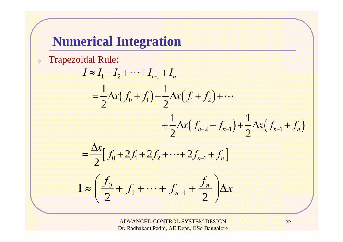
Numerical Integrationo Trapezoidal Rule:

( ) ( )

( ) ( )

[ ]

1 2 -1

0 1 1 2

2 1 1

0 1 2 1

1 12 2

1 12 2

2 2 22

n n

n n n n

n n

I I I I I

x f f x f f

x f f x f f

x f f f f f

− − −

−

≈ + + + +

= Δ + + Δ + +

+ Δ + + Δ +

Δ= + + + + +

01 1I

2 2n

nf ff f x−

⎛ ⎞≈ + + + + Δ⎜ ⎟⎝ ⎠

ADVANCED CONTROL SYSTEM DESIGN Dr. Radhakant Padhi, AE Dept., IISc-Bangalore

23

Ordinary Differential Equation (ODE)

Ordinary: only one independent variableDifferential Equation: unknown functions enter into the equation through its derivativesOrder: highest derivative in fDegree: exponent of the highest derivative

2

2

43

3

( ) ( ) ( ), , , 0

( ): ( ) 0

d e g re e = 4 ; o rd e r = 3

n

n

d x t d x t d x tf xd t d t d t

d x tE x a m p le x td t

⎛ ⎞=⎜ ⎟

⎝ ⎠

⎛ ⎞− =⎜ ⎟

⎝ ⎠

ADVANCED CONTROL SYSTEM DESIGN Dr. Radhakant Padhi, AE Dept., IISc-Bangalore

24

What Is Solution of ODE ??A problem involving ODE is not completely

specified by its equationODE has to be supplemented with boundary

conditions.Initial value problem: x is given at some starting

value ti , and it is desired to find at some final points tfor at some discrete list of points.

Two point boundary value problem: Boundary conditions are specified at more than one t ; typically some of the conditions will be specified at ti and some at tf .

ADVANCED CONTROL SYSTEM DESIGN Dr. Radhakant Padhi, AE Dept., IISc-Bangalore

25

Numerical Solution to Initial Value Problem

A numerical solution to this problem generates sequence of values for the independent variable t1,t2,…tn and a corresponding sequence of values of the dependent variable x1,x2….,xn so that eachxn approximates solution at tn

xn ≈ x (tn) n=0,1,2….n.

0 0( ) ( , ( )); ( )dx t f t x t x t x

dt= =

ADVANCED CONTROL SYSTEM DESIGN Dr. Radhakant Padhi, AE Dept., IISc-Bangalore

26

Basic Concepts of Numerical Methods to Solve ODEs

1 slope of tangentn nx xt

+ −≈

ΔWe can calculate the tangent slope at any point. In fact the differential equation

( )

( )

( ) , ( ) defines the

tangent slope , ( )

dx t f t x tdt

f t x t

=

=

ADVANCED CONTROL SYSTEM DESIGN Dr. Radhakant Padhi, AE Dept., IISc-Bangalore

27

Euler’s MethodSolve with

At start of time step

Forward difference

Start with initial conditions t0=0; x0=b

( , )dx f t xdt

= (0)x b=

1

1

( , )

Rearranging

n nn n

n n n

x x f t xt

x x t f

+

+

−≈

Δ

= + Δ

ADVANCED CONTROL SYSTEM DESIGN Dr. Radhakant Padhi, AE Dept., IISc-Bangalore

28

• Euler integration has error of the order of

• Small step size may be needed for good accuracy. This is in conflict with the computational load advantage.

• Lesser computational load

tΔ

Euler Integration: Useful Comments

( )2tΔ

ADVANCED CONTROL SYSTEM DESIGN Dr. Radhakant Padhi, AE Dept., IISc-Bangalore

29

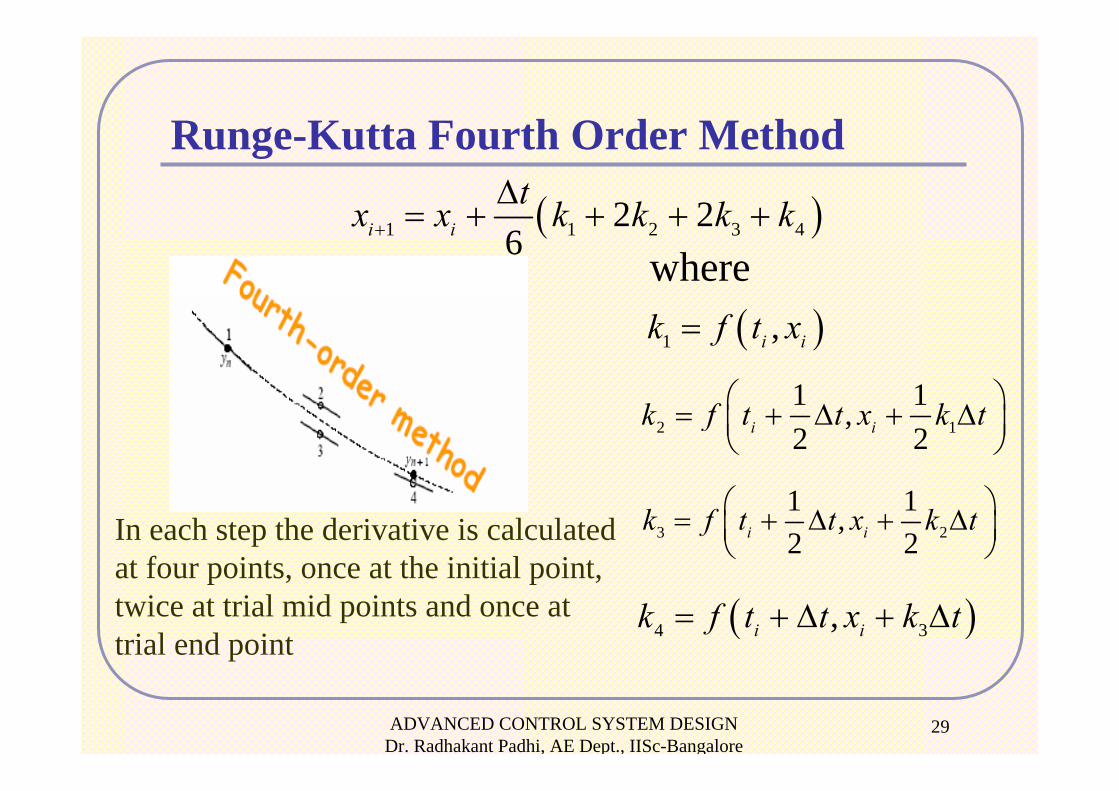
Runge-Kutta Fourth Order Method

where( )1 ,i ik f t x=

2 1

1 1,2 2i ik f t t x k t⎛ ⎞= + Δ + Δ⎜ ⎟

⎝ ⎠

3 2

1 1,2 2i ik f t t x k t⎛ ⎞= + Δ + Δ⎜ ⎟

⎝ ⎠

( )4 3,i ik f t t x k t= + Δ + Δ

( )1 1 2 3 42 26i i

tx x k k k k+

Δ= + + + +

In each step the derivative is calculated at four points, once at the initial point, twice at trial mid points and once at trial end point

ADVANCED CONTROL SYSTEM DESIGN Dr. Radhakant Padhi, AE Dept., IISc-Bangalore

30

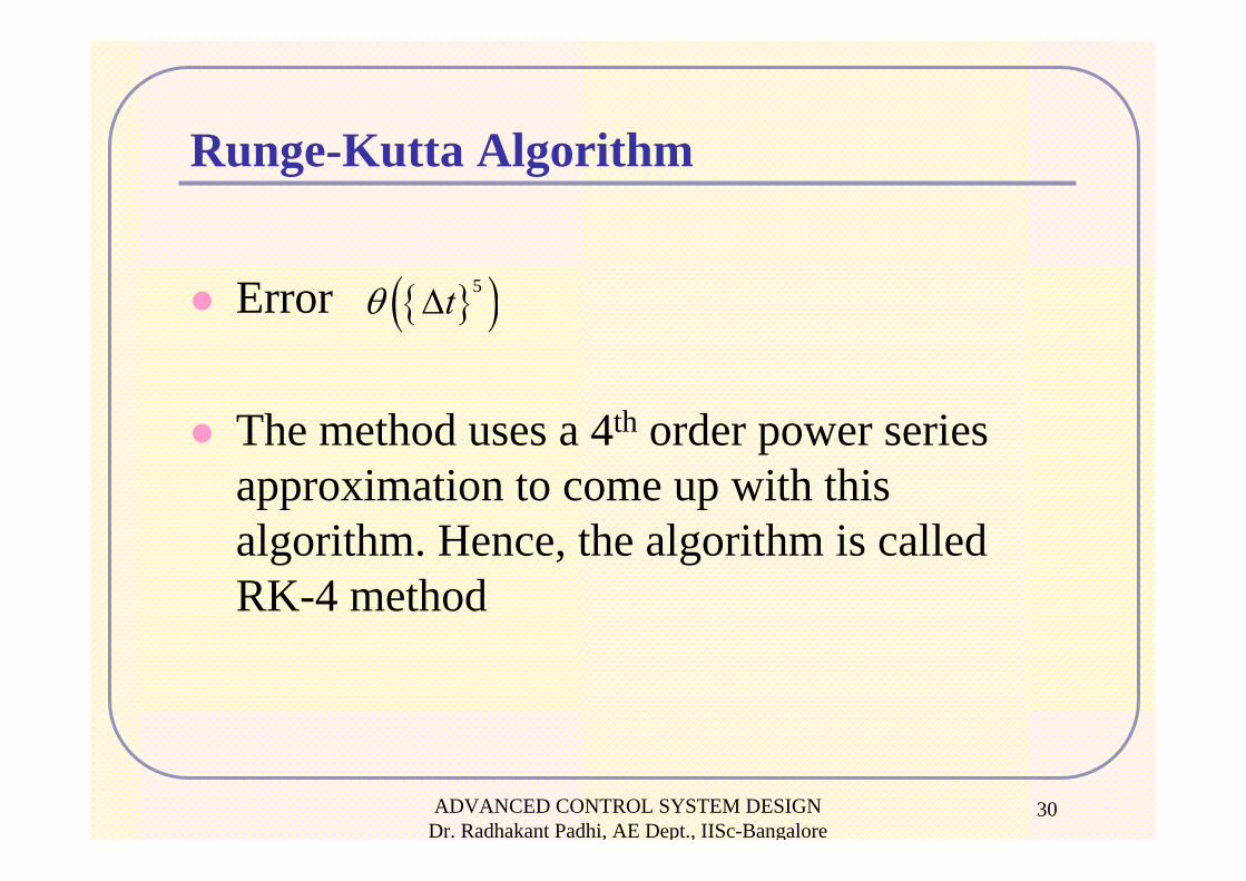
{ }( )5tθ Δ

Runge-Kutta Algorithm

Error

The method uses a 4th order power series approximation to come up with this algorithm. Hence, the algorithm is called RK-4 method

ADVANCED CONTROL SYSTEM DESIGN Dr. Radhakant Padhi, AE Dept., IISc-Bangalore

31

ADVANCED CONTROL SYSTEM DESIGN Dr. Radhakant Padhi, AE Dept., IISc-Bangalore

32